Welding Robot Collision-Free Path Optimization


Key Laboratory of Advanced Control and Optimization for Chemical Processes of Ministry of Education, East China University of Science and Technology, Shanghai 200237, China
*
Author to whom correspondence should be addressed.
Appl. Sci. 2017, 7(2), 89; https://doi.org/10.3390/app7020089
Submission received: 10 November 2016
/
Accepted: 11 January 2017
/
Published: 8 February 2017
(This article belongs to the Special Issue Gas Tungsten Arc Welding)
Abstract
:Reasonable welding path has a significant impact on welding efficiency, and a collision-free path should be considered first in the process of welding robot path planning. The shortest path length is considered as an optimization objective, and obstacle avoidance is considered as the constraint condition in this paper. First, a grid method is used as a modeling method after the optimization objective is analyzed. For local collision-free path planning, an ant colony algorithm is selected as the search strategy. Then, to overcome the shortcomings of the ant colony algorithm, a secondary optimization is presented to improve the optimization performance. Finally, the particle swarm optimization algorithm is used to realize global path planning. Simulation results show that the desired welding path can be obtained based on the optimization strategy.
1. Introduction
With developments in welding technology, computer technology and robot technology, welding robots have been widely used in industrial production, especially in the automotive sector. To improve welding productivity when there are many weld joints, robot path planning needs to be studied. For welding robot path planning, some factors should be considered. Optimization objectives include a minimum path length [1], collision-free paths [2], and welding deformation [3].
Obstacle avoidance is a fundamental problem in welding robot path planning. However, most path planning with obstacle avoidance is obtained based on teaching mode programming. In this way, the planning process is time-consuming, and the optimum path is hard to achieve. Hence, robot collision-free path planning based on optimization algorithms needs to be studied to improve welding efficiency. Collision-free path planning includes two stages: environment modeling and path searching, which are explained in the following paragraphs.
Environment modeling refers to the mathematical description of the environment around the welding robot, which is essential for collision-free path planning. Allan [4] applied a grid method to solve path planning for real-time robots in dynamic environments. For the grid method, grids are applied to describe the free space and obstacle space in the robot’s work space. A good path can be achieved if the precision is high, but the algorithm would be time-consuming at the same time. The environment would not be described clearly if the precision were otherwise low. Yu [5] presented a C-space layered search arithmetic for manipulators. Although the method could achieve obstacle avoidance for robot arms, the obstacle modeling was complex and inefficient. With increases in robot freedom, the computation becomes very complicated. In addition, there are other environmental modeling methods, such as the visibility graph method [6], the bounding box method [7], artificial neural networks [8], and approximate voronoi boundary networks [9].
After environment modeling, some path searching methods are essential to find an appropriate path. Li [10] presented an improved APF-based SIFORS method for autonomous mobile robot path planning in complex environments. The artificial potential field method is straightforward, but some problems may exist, such as the local optimum problem, falling into a deadlock, and moving unsteadily near the obstacle. Cao [11] proposed an improved ant colony algorithm for robot global path planning; the pheromone evaporation rate was adjusted dynamically to enhance the global search ability and convergence speed. In addition, the artificial bee colony algorithm [12] and the genetic algorithm [13] are also used to search the optimum path.
In this paper, obstacle avoidance and path length are considered to optimize path. Based on the above analysis, the model description is first described in Section 2. Then, in Section 3, the grid method is selected to realize environment modeling. Moreover, the ant colony algorithm (ACO) is applied for path searching in Section 4. In addition to this, a particle warm optimization (PSO) algorithm is used to realize global optimization in Section 5. Finally, conclusions are given in Section 6.
2. Model Description of Welding Robot Path Planning with Obstacle Avoidance
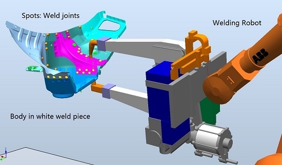
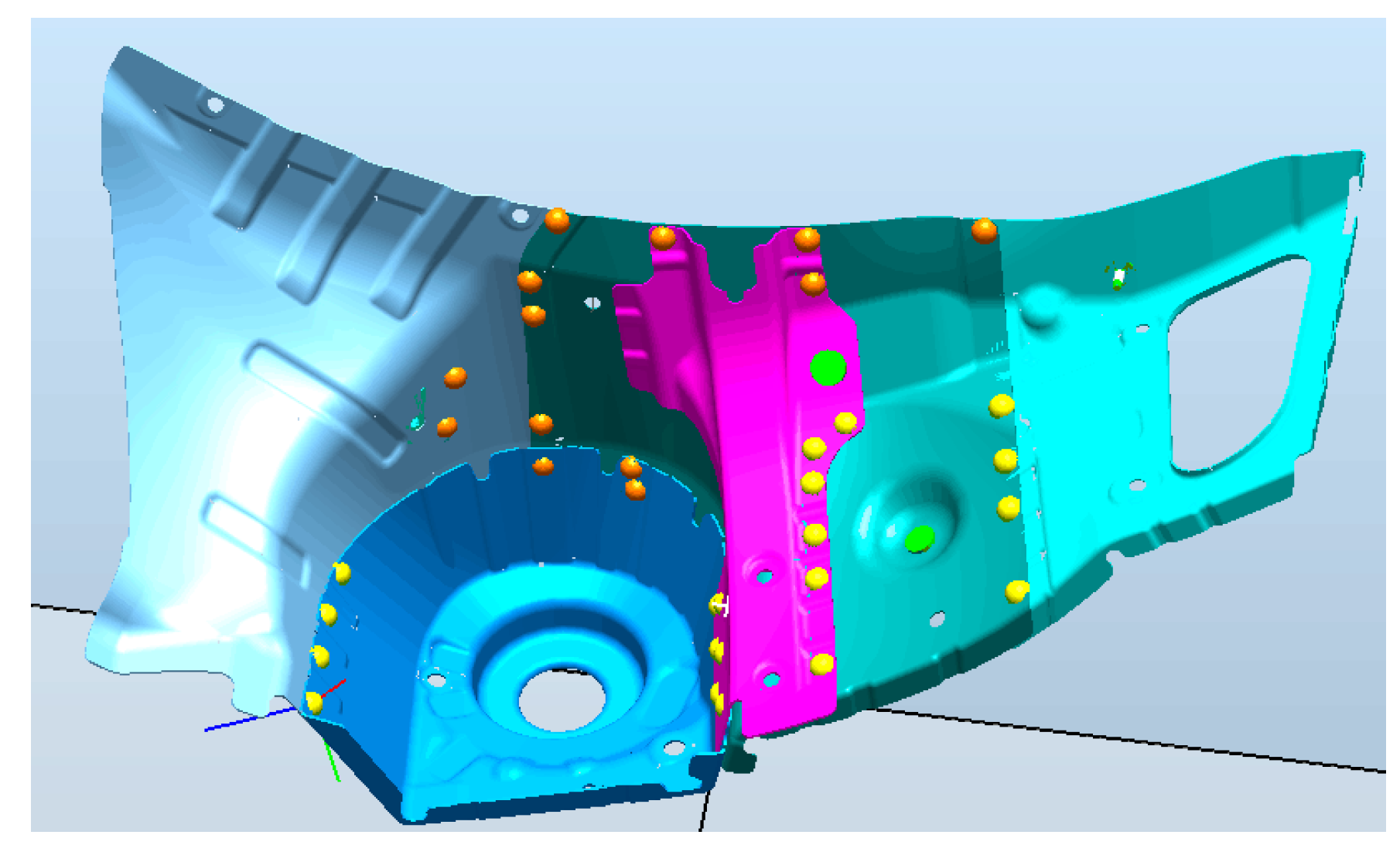
Because spot welding robots are widely used for car body in white, it was selected as the welding object in this paper. All weld joints are given as spots, which are shown in Figure 1. To illustrate the problem more clearly, parts of the weld joints are chosen to conduct path planning, which are shown in Figure 2. The coordinates of 15 weld joints were obtained in “RobotStudio” software and are shown in Table 1.
In order to achieve welding robot path planning with a collision-free path, a welding torch should move through all the weld joints first. At the same time, the shortest path length possible and the avoidance of all obstacles in the environment are desired. Suppose the number of the weld joints is , the welding sequence is . Then, the problem can be treated as a TSP (Traveling Salesman Problem) with constraint conditions. TSP is described as follows. Suppose a salesman has to visit cities with the conditions that he must visit each city only once and finally return to the original departure city. The path planning problem can be described as
where is the path between Weld Joints , which represents the local path. The welding sequence represents the global path.
For the path between two weld joints, the welding torch moves through intermediate points to avoid the obstacle and suppose that the path between weld joints and the intermediate points are straight lines. If the starting point is , the terminal point is , and the intermediate points are . Path is made up of , and the planning of can be described as follows:
where indicates the Euclidean distance between point and . XY is a safe path, which represents that the robot’s moves from point X to point without collision.
3. 3D Environment Modeling
For collision-free path planning, the environment model of robot should be established. The grid method is relatively simple and intuitive when used for map creation and is beneficial for detecting the environment in the path searching process. Hence, the grid method is selected as the modeling method in this paper. Because the traditional grid method is used in 2D space, while the working environment for the welding robot is in 3D space, the improvement of the grid method is necessary. The procedure of the 3D environment modeling with the grid method is presented as follows.
- (1)
- (2)
- Set up grid matrix. The whole space is divided into small cubes, and the centers of the cubes are set as the welding torch’s footholds (Figure 4). Because the diameter of the welding electrode is 4.48 mm, each side length of the cubes is set to 5 mm. Then, all centers of the cubes are mapped on the triangles. If the projected point is located in the triangle and the vertical length is less than 5 mm, the triangle is the obstacle for the center; otherwise, the triangle is not the obstacle for the center.
- (3)
- If there are no obstacle triangles for a center, the center is a free point. Otherwise, the center is an obstacle point, which means that the welding torch cannot be located in the point.
- (4)
- Because the actual weld joints are located on the surface of the weldment, the weld joints cannot be located in the free points. However, in the process of path planning, the welding torch can only move among the free points. To solve this problem, a nearest free point is defined as a virtual weld joint for the weld joint. Because the distance between actual weld joints and virtual weld joints is invariable and is small in terms of the whole path length, the distance is ignored in the optimization process. The path planning mentioned below only considers the path between the virtual weld joints.
4. Collision Free Path Optimization
4.1. Ant Colony Optimization Algorithm (ACO)
ACO is a swarm intelligence optimization algorithm that stems from real ants. In 1991, Dorigo [14] firstly proposed the ACO and successfully applied it for solving different combination optimization problems. The foraging behavior of the ant colony can be regarded as a distributed collaborative optimization mechanism. It is difficult to find the shortest path from the nest to the food source for a single ant, while the ant colony can find the shortest path because the ants can communicate with each other by releasing pheromones on the route passed. The basic ACO mode is presented as follows [14]:
where is the transition probability of ant from to , is the location of the ant, and is the location that the ant can arrive at. is the pheromone intensity from to , and is heuristic information, where . is the weight of the pheromone, is the weight of heuristic information, is the collection of the nodes that ants can reach, and is the evaporation coefficient of pheromone on the route. is the pheromone intensity ant leaves on the route from to , and is the amounts of ants. is the number of iterations, is the objective function, which is the Euclidean distance between two points, is the quality coefficient of the pheromone, and is path length of ant goes from nest to food source.
4.2. Collision Free Path Optimization Based on ACO
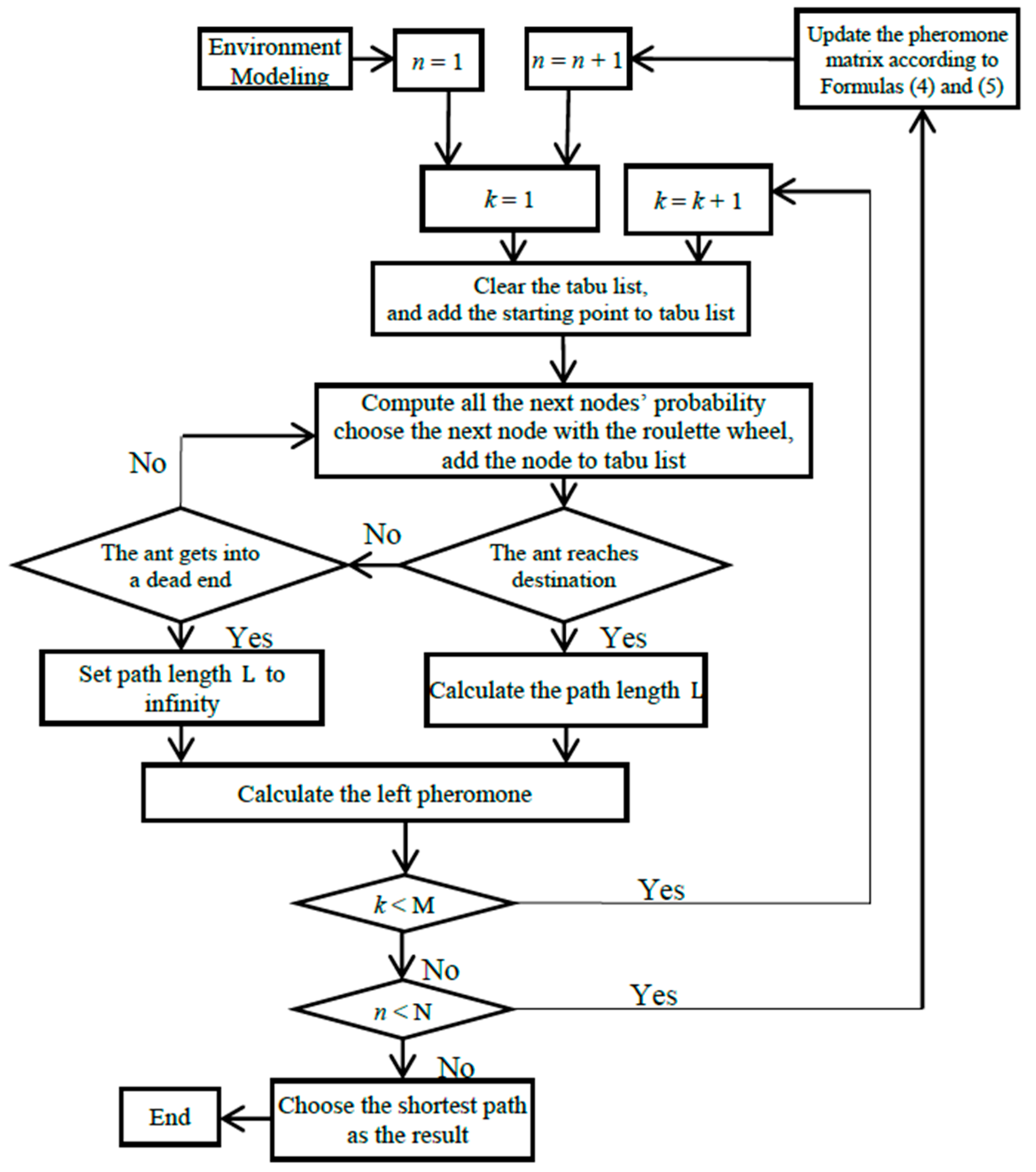
When the ACO is applied for the welding robot path planning, the starting point of the welding torch is the nest of the ant colony and the destination is the food resource. Hence, the path planning based on the ACO is the food searching process for the ant colony. The communication between the ants is realized based on pheromones. The shortest path can be found through the mutual cooperation among the individuals. The chart of the welding robot local path planning is shown in Figure 5.
Steps of the local welding path planning with collision-free based on ACO are given as follows:
Step 1. Realize the environment modeling based on the grid method.
Step 2. Initialize the parameters of the ACO. Based on the empirical value, the weight of the pheromone is set as 1, the weight of heuristic pheromone is set as 11, the evaporation coefficient of pheromone is set as 0.9, and the pheromone quality coefficient Q is set as 5. The iteration number N is set as 50, and the population quantity M is set as 50. Initialize the coordinates of the starting point and the terminal point. Initialize the pheromone matrix, and the pheromones for all points are set as 0.5. The above parameter settings are shown in Table 2.
Step 3. Set iterator as 1.
Step 4. Set the number of ant as 1.
Step 5. Clear tabu list for the ant , add the starting point to , and clear foraging path for ant .
Step 6. Calculate the probability of each node according to Equation (3). In this paper, the ants’ step length is set as 5 mm and the number of nodes that can be chosen as the next node is no larger than 6. The positive and negative directions of the 3D coordinate system are set as the directions of the ants’ movement in this paper. Hence, the number of directions of the ants’ movement is 6. When there are neighboring nodes that are obstacle points, the number of next nodes that the ant can choose is lower than 6. Select the next node according to the roulette wheel and add the node to the list and foraging path .
Step 7. If the ant reaches the destination or reaches a dead end, jump to Step 8. Otherwise, return to Step 6. A dead end means that, for the current node, there are not any nodes that can be found as the next node.
Step 8. If the ant reaches the destination, calculate the path length according to Equation (2). If the ant reaches a dead end, the path length is set to infinity. Calculate the left pheromone according to Equations (4) and (5).
Step 9. If is less than , , and return to Step 5. Otherwise, jump to Step 10.
Step 10. Update the pheromone matrix according to Equations (4) and (5).
Step 11. If , , and return to Step 4. Otherwise, jump to Step 12.
Step 12. Select the shortest foraging path (), which is the result of collision-free welding path planning.
4.3. The Secondary Optimization of ACO (SO-ACO)
The path solved based on the ACO is not the shortest path because of its discontinuous step length and direction. Hence, a secondary optimization (SO) is proposed to obtain better optimization results. Here, represents the optimized path based on ACO, and represents improved path based on SO-ACO. The optimization process is presented as follows:
Step 1. Initialize as void.
Step 2. Add the first point of to .
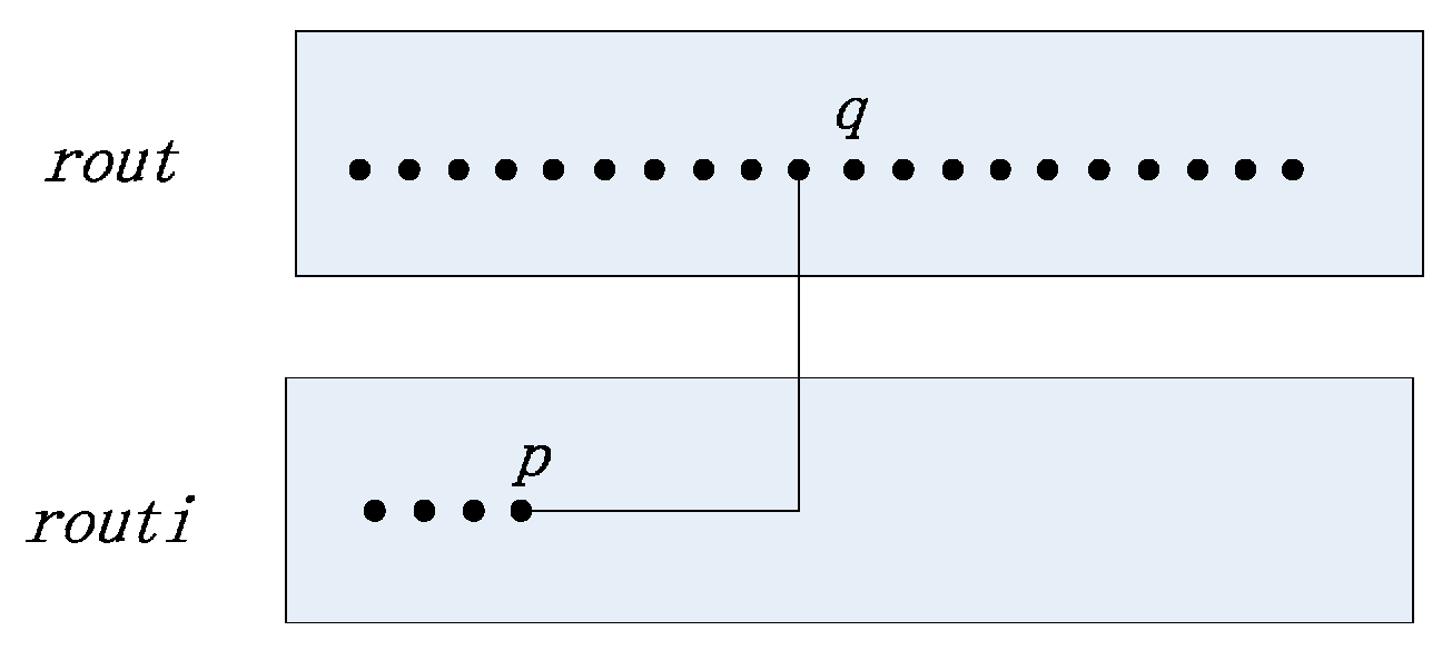
Step 3. Suppose the last point of is , and the last point in is .
Step 4. If is the next point to , the location of in and in are shown in Figure 8, jump to Step 6. Otherwise, jump to Step 5.
Step 5. Connect and to form a line. If the line encounters the obstacles, set the point in front of in as , and return to Step 4. Otherwise, jump to Step 6.
Step 6. Add to .
Step 7. If is the last point in , jump to Step 8; otherwise, return to Step 3.
Step 8. Compare the length of and . If the length is the same, jump to Step 10. Otherwise, replace the sequence in with that in and jump to Step 9.
Step 9. If the length of each segment in is greater than 5 mm, the segment is split into points, and the new points are added to . Then, reverse the order of the and return to Step 1.
Step 10. Set as the optimized result.
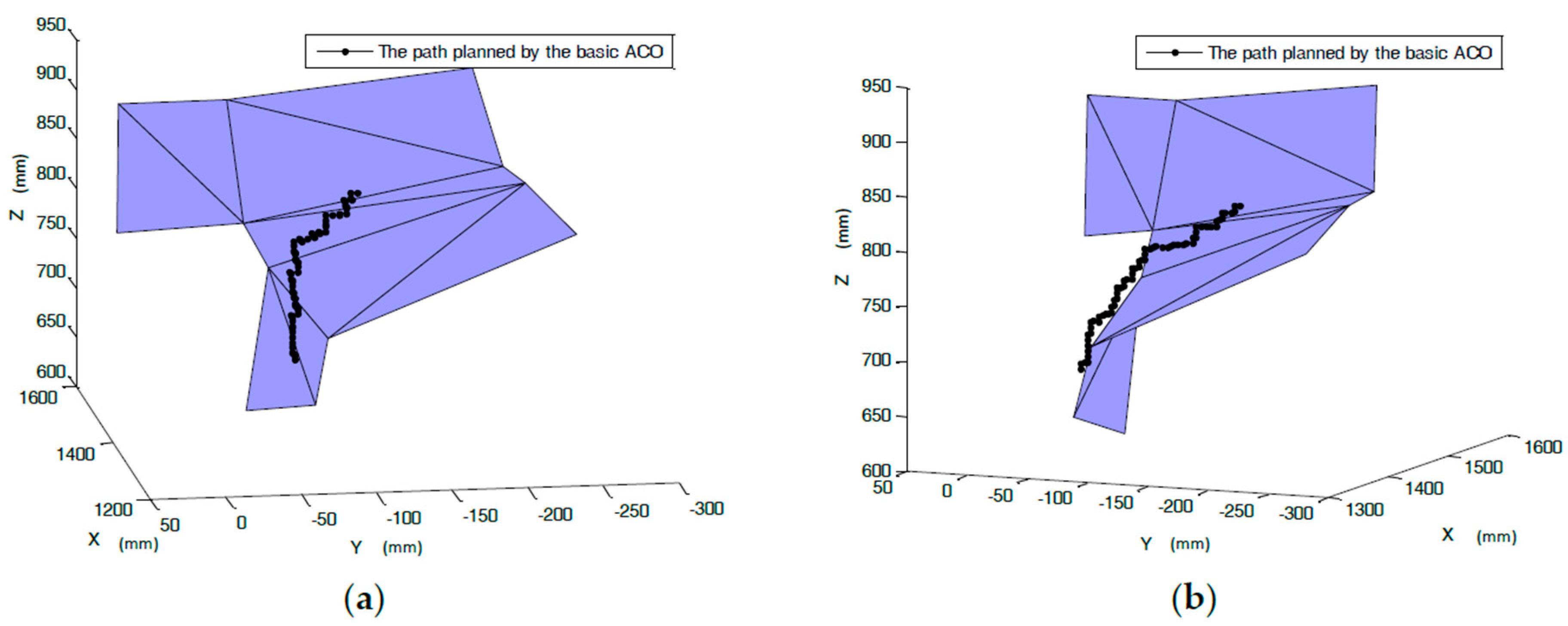
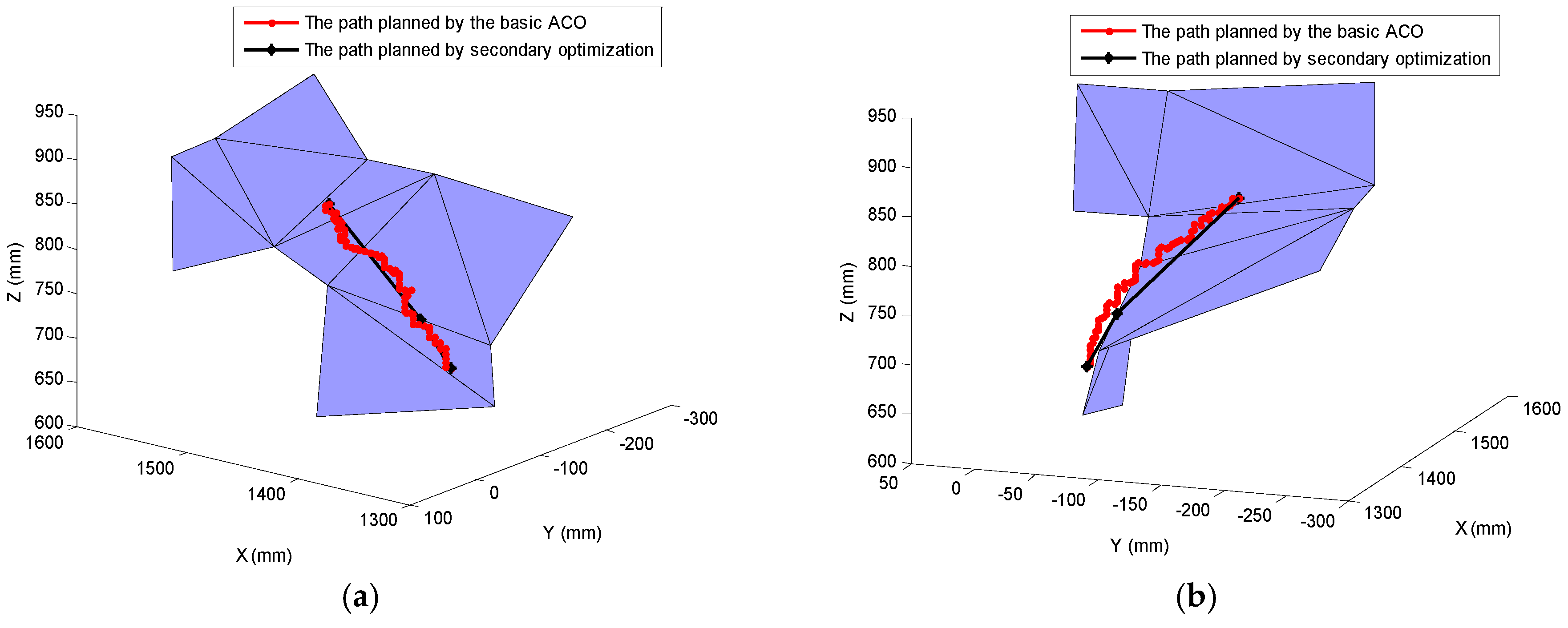
According to the above steps, when the Weld Joints 3 and 7 are selected as the starting joint and the terminal joint, respectively, the parameters of the ACO are the same as Section 4.2. The path planning result based on the SO-ACO is shown in Figure 9 (a and b are a different view of the same result). The path length optimized based on ACO is 330 mm, while the path length optimized based on the SO-ACO is 203.290 mm.
Different iterations and population sizes are selected to prove the effectiveness of the SO-ACO, which are shown in Table 3. Other parameters refer to Section 4.2. The algorithm is conducted 20 times for every condition, and the minimum, maximum, average, variance of path length, and time for every conditions are shown in Table 3.
From Table 3, it can be seen that the SO-ACO is obviously superior to the basic ACO; satisfactory results were obtained when the iterations and population sizes were 10. For ACO, with the increase in the iteration , population size , and searching time, the path length of the ACO decreases, but it is still larger than the optimization results based on SO-ACO. Hence, it can be concluded that the SO-ACO can improve the optimization effect of the algorithm, and it can be applied for actual optimization processes to achieve a satisfactory result with a small iteration and population size .
5. Global Welding Robot Path Planning
Based on the collision free path optimization, the global welding path planning can be treated as a TSP. Due to the effective application of the PSO, this algorithm will be used to realize global optimization for welding robot path.
5.1. Particle Swarm Optimization Algorithm
In 1995, Kennedy and Eberhart [15] presented the particle swarm optimization (PSO) algorithm based on the regularity of hunting birds. In the PSO algorithm, every bird is named as a particle with no quality and volume. Multiple particles coexist and search for the best position with cooperation. Every particle moves to a better position with its experience and others’ in the swarm. The best position of a particle is called , and the best position of the whole swarm is called . The state of the particle is described by the d-dimensional velocity and the position . Thus, every particle updates its state according to Equations (6) and (7), and the next generation is generated.
where represents the current iterations. , , which are the learning factor, are usually positive and adjust the traction force of the personal optimal position and the global optimal position. are random numbers between 0 and 1.
The PSO algorithm has shown its superior performance in optimization of continuous problems. However, the original PSO is not appropriate for solving discrete problems such as TSP. Clerc [16] proposed a TSP-PSO algorithm based on the operation of particle positions and velocity vector to solve TSP. This algorithm is used to realize global path planning in Section 5.2.
5.2. Global Path Planning Based on PSO
Because of the advantages of PSO, it is chosen as the optimization algorithm for global path planning. The steps of the globe welding path planning based on PSO are presented as follows [16]:
Step 1. Initialization: the iterations N of the PSO is set as 100, the population size is set as 50, and the learning rates , are set as 1.0. The weight is set as 0.4. The positions and velocities of the particles are initialized randomly. The local route can be obtained according to the local path planning algorithm. Each particle’s fitness is evaluated in the light of Equations (6) and (7). Then, the personal best positions and the global best position of the particles are updated. The above parameter settings are shown in Table 4.
Step 2. Update the positions and velocities of the particles according to the equation of the PSO. Update the fitness, personal best positions, and the global best position.
Step 3. If the number of iterations is not larger than 100, then return to Step 2; otherwise, jump to Step 4.
Step 4. The global best position is the result of the global welding path planning.
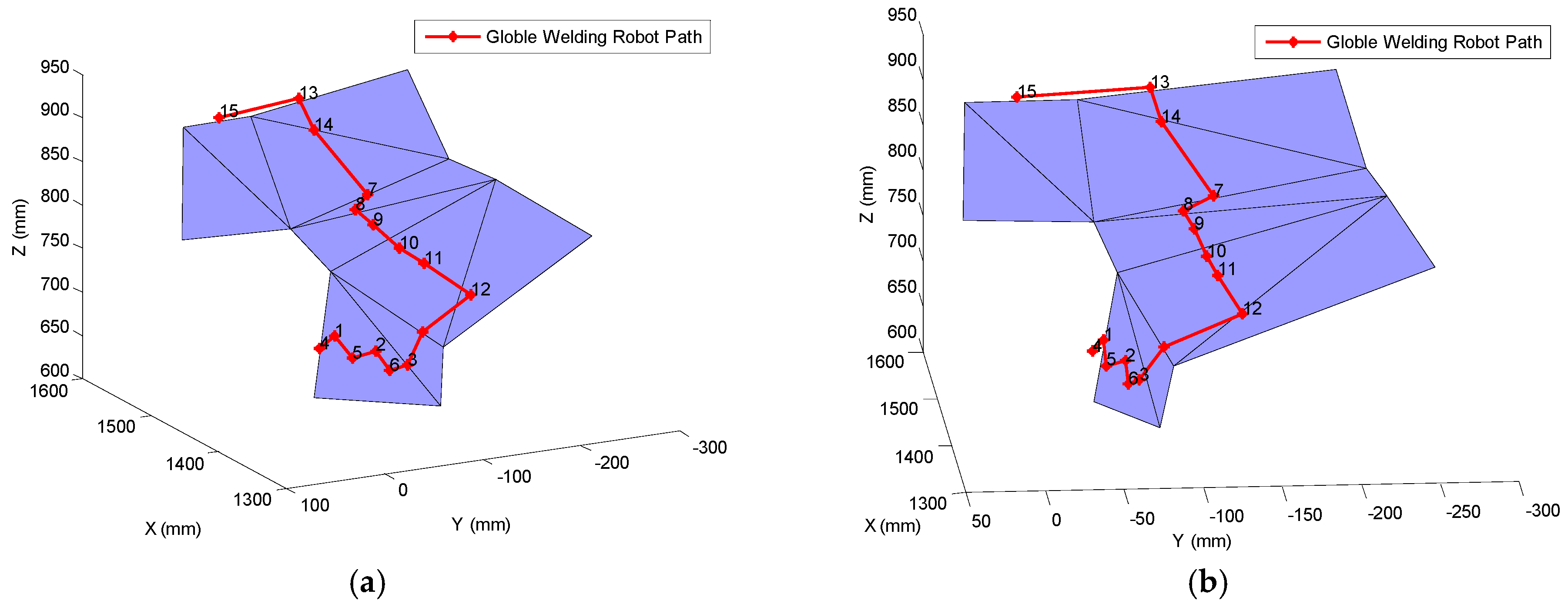
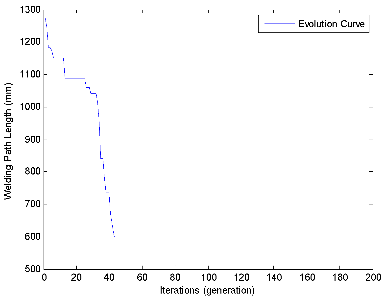
Based on the above steps, the shortest collision-free welding path can be achieved as follows: 15→13→14→7→8→9→10→11→12→3→6→2→5→1→4. The global path length is 599.720 mm, the final global welding collision-free robot path planning is shown in Figure 10, and the iterative process of PSO is shown in Figure 11.
6. Conclusions
Welding robot collision-free path optimization was studied in this paper. The optimization objective is the shortest path length and the constraint is obstacle avoidance. Environment modeling was realized using the grid method. The ACO was used for path searching. In order to improve the performance of the ACO, a secondary optimization algorithm was presented, which markedly improves the result of the algorithm. Finally, particle swarm optimization was applied to optimize the global welding collision-free path planning. The shortest collision-free path was obtained based on the proposed strategies in this paper, which shows the effectiveness of the algorithm.
The welding path optimization studied in this article is similar to practical welding situations. Hence, manual teaching and offline programming (OLP) is beneficial. Based on the optimization strategy, the obtained welding path can help welding engineering by shortening the teaching time. At the same time, the path can make the OLP software intelligent and more effective after the optimization strategy is integrated with OLP software.
Acknowledgments
The authors appreciate the support of the Shanghai Natural Science Foundation (14ZR1409900) and the National Natural Science Foundation of China (61573144, 61673175).
Author Contributions
Xuewu Wang and Lika Xue conceived and designed the optimization strategy; Lika Xue performed the simulations; Yixin Yan and Xingsheng Gu offered help for the simulations; Xuewu Wang and Lika Xue wrote the paper.
Conflicts of Interest
The authors declare no conflict of interest.
References
- Wang, X.; Shi, Y.; Ding, D.; Gu, X. Double global optimum genetic algorithm-particle swarm optimization-based welding robot path planning. Eng. Optim. 2016, 48, 299–316. [Google Scholar] [CrossRef]
- Ramer, C.; Reitelshofer, S.; Franke, J. A robot motion planner for 6-DOF industrial robots based on the cell decomposition of the workspace. In Proceedings of the 2013 44th International Symposium on Robotics (ISR), Seoul, Korea, 24–26 October 2013; IEEE: New York, NY, USA, 2013; pp. 1–4. [Google Scholar]
- Yang, H.; Shao, H. Distortion-oriented welding path optimization based on elastic net method and genetic algorithm. J. Mater. Process. Technol. 2009, 209, 407–412. [Google Scholar] [CrossRef]
- Willms, A.R.; Yang, S.X. Real-time robot path planning via a distance-propagating dynamic system with obstacle clearance. IEEE Trans. Syst. Man Cybern. B Cybern. 2008, 38, 884–893. [Google Scholar] [CrossRef] [PubMed]
- Yu, N.; Wang, Z. Collision avoidance planning of manipulator based on C-space layered search arithmetic. In Proceedings of the 2011 International Conference on Electronic and Mechanical Engineering and Information Technology (EMEIT), Harbin, China, 12–14 August 2011; IEEE: New York, NY, USA, 2011; Volume 6, pp. 3258–3262. [Google Scholar]
- Masehian, E.; Amin Naseri, M.R. A voronoi diagram-visibility graph-potential field compound algorithm for robot path planning. J. Robot. Syst. 2004, 21, 275–300. [Google Scholar] [CrossRef]
- Teschner, M.; Kimmerle, S.; Heidelberger, B.; Zachmann, G.; Raghupathi, L.; Fuhrmann, A.; Cani, M.-P.; Faure, F.; Magnenat-Thalmann, N.; Strasser, W.; et al. Collision detection for deformable objects. In Computer Graphics Forum; Blackwell Publishing Ltd.: Oxford, UK, 2005; Volume 24, pp. 61–81. [Google Scholar]
- Duan, H.; Huang, L. Imperialist competitive algorithm optimized artificial neural networks for UCAV global path planning. Neurocomputing 2014, 125, 166–171. [Google Scholar] [CrossRef]
- Mo, H.; Xu, L. Research of biogeography particle swarm optimization for robot path planning. Neuro Comput. 2015, 148, 91–99. [Google Scholar] [CrossRef]
- Li, G.; Tong, S.; Cong, F.; Yamashita, A.; Asama, H. Improved artificial potential field-based simultaneous forward search method for robot path planning in complex environment. In Proceedings of the 2015 IEEE/SICE International Symposium on System Integration (SII), Nagoya, Japan, 11–13 December 2015; IEEE: New York, NY, USA, 2015; pp. 760–765. [Google Scholar]
- Cao, J. Robot Global Path Planning Based on an Improved Ant Colony Algorithm. J. Comput. Commun. 2016, 4, 11–19. [Google Scholar] [CrossRef]
- Lei, L.; Shiru, Q. Path planning for unmanned air vehicles using an improved artificial bee colony algorithm. In Proceedings of the 2012 31st Chinese Control Conference (CCC), Hefei, China, 25–27 July 2012; IEEE: New York, NY, USA, 2012; pp. 2486–2491. [Google Scholar]
- Wang, Y.; Mulvaney, D.; Sillitoe, I. Genetic-based mobile robot path planning using vertex heuristics. In Proceedings of the 2006 IEEE Conference on Cybernetics and Intelligent Systems, Bangkok, Thailand, 7–9 June 2006; IEEE: New York, NY, USA, 2006; pp. 1–6. [Google Scholar]
- Colorni, A.; Dorigo, M.; Maniezzo, V. Distributed optimization by ant colonies. In Proceedings of the First European Conference on Artificial Life, Paris, France, 13 December 1991; Volume 142, pp. 134–142.
- Kennedy, J.; Eberhart, R.C. Particle swarm optimization. In Proceedings of the IEEE International Conference on Neural Networks, Perth, Australia, 27 November–1 December 1995; IEEE: New York, NY, USA, 1995; pp. 1942–1948. [Google Scholar]
- Clerc, M. Discrete particle swarm optimization, illustrated by the traveling salesman problem. In New Optimization Techniques in Engineering; Springer: Berlin/Heidelberg, Germany, 2004; pp. 219–239. [Google Scholar]
Figure 1.
Body in white weld piece.

Figure 2.
Part of the body in white weld piece.
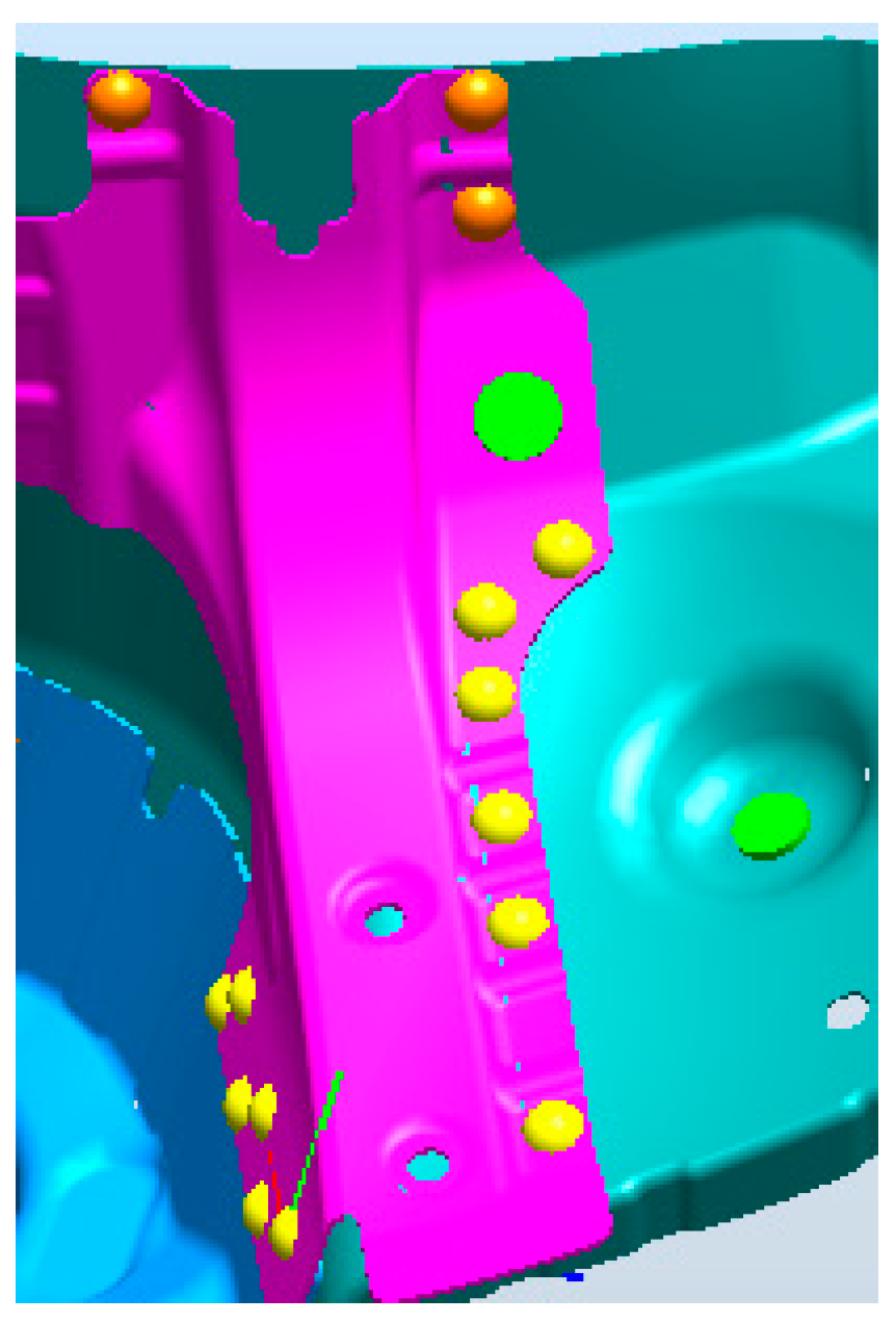
Figure 3.
Simplified triangles for white body weld piece, red spots: weld joints.
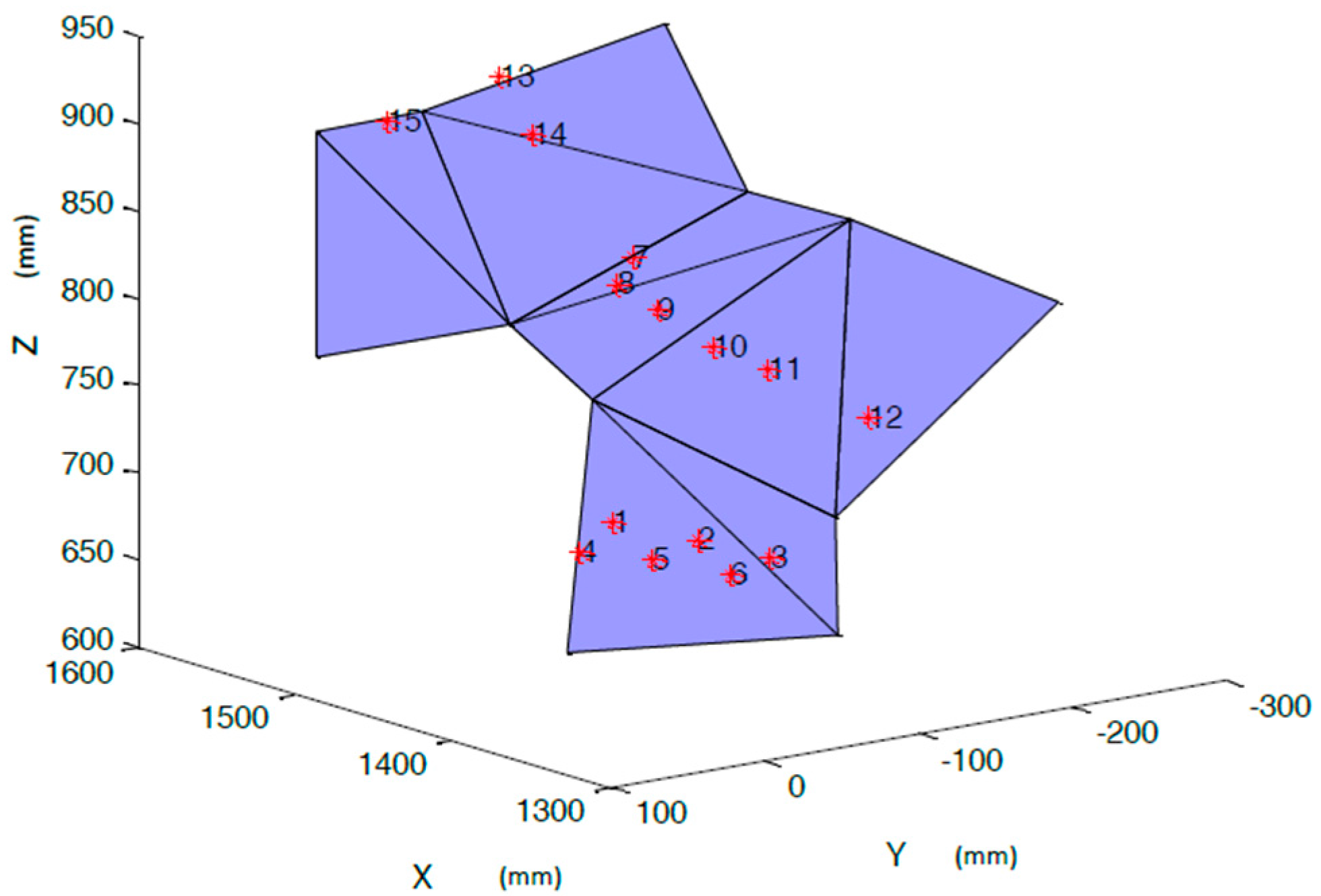
Figure 4.
The environment model using the grid method, red spots: weld joints, blue area: grid matrix.
Figure 4.
The environment model using the grid method, red spots: weld joints, blue area: grid matrix.
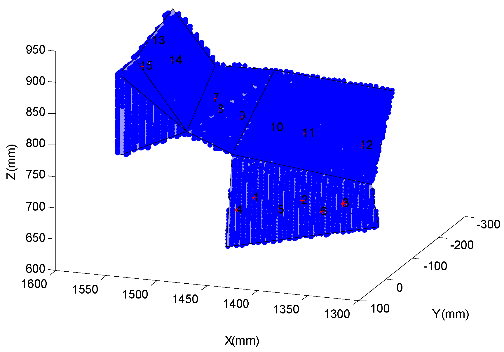
Figure 5.
Chart of welding robot collision free path optimization.

Figure 6.
Welding robot path planning between two weld joints. (a) View A; (b) View B.

Figure 7.
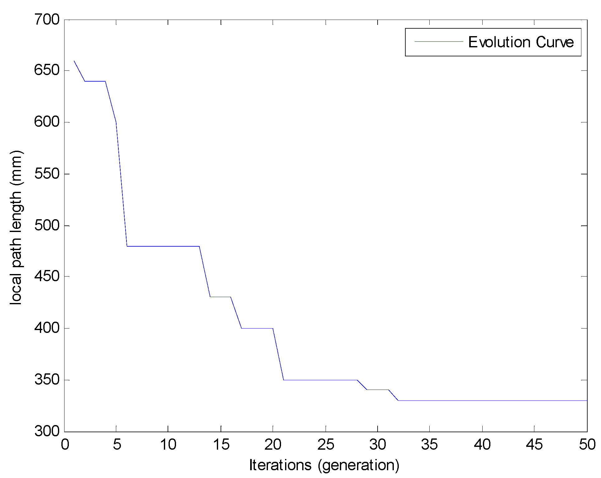
The iterative process of the ant colony algorithm.

Figure 8.
The location of and .

Figure 9.
Welding robot path planning based on the Secondary Optimization of ACO (SO-ACO). (a) View A; (b) View B.
Figure 9.
Welding robot path planning based on the Secondary Optimization of ACO (SO-ACO). (a) View A; (b) View B.

Figure 10.
Global path planning with obstacle avoidance. (a)View A; (b) View B.

Figure 11.
Iterative process of particle swarm optimization.


| NO. | X (mm) | Y (mm) | Z (mm) | NO. | X (mm) | Y (mm) | Z (mm) |
|---|---|---|---|---|---|---|---|
| 1 | 1443.60 | −53.20 | 686.00 | 9 | 1474.16 | −111.25 | 791.00 |
| 2 | 1399.56 | −60.05 | 688.49 | 10 | 1442.88 | −117.47 | 779.19 |
| 3 | 1356.00 | −66.67 | 689.57 | 11 | 1414.82 | −122.26 | 771.35 |
| 4 | 1456.36 | −48.49 | 669.34 | 12 | 1356.71 | −132.48 | 759.65 |
| 5 | 1417.70 | −54.51 | 671.94 | 13 | 1554.17 | −94.37 | 909.95 |
| 6 | 1379.31 | −60.57 | 674.61 | 14 | 1539.25 | −99.03 | 879.83 |
| 7 | 1504.91 | −126.99 | 813.51 | 15 | 1549.76 | −8.79 | 903.34 |
| 8 | 1493.74 | −109.17 | 801.14 | - | - | - | - |
| Q | N | M | Initial Pheromone | |||
|---|---|---|---|---|---|---|
| 1 | 11 | 0.9 | 5 | 50 | 50 | 0.5 |
| N | M | Method | Path Length L (mm) | Time t (s) | ||||||
|---|---|---|---|---|---|---|---|---|---|---|
| Mean | SD | Min | Max | Mean | SD | Min | Max | |||
| 5 | 5 | ACO | 681.000 | 97.002 | 560.000 | 910.000 | 1.094 | 0.105 | 0.909 | 1.294 |
| SO-ACO | 206.326 | 8.760 | 202.507 | 242.524 | 1.242 | 0.102 | 1.066 | 1.403 | ||
| 10 | 10 | ACO | 579.500 | 55.864 | 490.000 | 670.000 | 4.234 | 0.286 | 3.739 | 4.950 |
| SO-ACO | 203.085 | 0.617 | 202.390 | 204.582 | 4.369 | 0.303 | 3.844 | 5.098 | ||
| 20 | 20 | ACO | 460.500 | 33.162 | 400.000 | 530.000 | 13.391 | 0.440 | 12.672 | 14.584 |
| SO-ACO | 203.219 | 0.931 | 202.390 | 206.187 | 13.511 | 0.436 | 12.783 | 14.676 | ||
| 30 | 30 | ACO | 361.000 | 12.937 | 340.000 | 390.000 | 25.038 | 0.901 | 23.776 | 28.028 |
| SO | 203.039 | 0.770 | 202.507 | 205.451 | 25.152 | 0.893 | 23.901 | 28.122 | ||
| 40 | 40 | ACO | 330.500 | 2.236 | 330.000 | 340.000 | 43.199 | 2.118 | 38.954 | 47.122 |
| SO-ACO | 202.930 | 0.357 | 202.370 | 203.426 | 43.332 | 2.125 | 39.063 | 47.263 | ||
| 50 | 50 | ACO | 330.000 | 0.000 | 330.000 | 330.000 | 56.213 | 3.892 | 50.827 | 68.322 |
| SO-ACO | 203.120 | 1.069 | 202.390 | 206.187 | 56.340 | 3.901 | 50.930 | 68.468 | ||
| 60 | 60 | ACO | 330.000 | 0.000 | 330.000 | 330.000 | 76.361 | 6.807 | 65.979 | 89.289 |
| SO-ACO | 202.800 | 0.477 | 202.390 | 204.443 | 76.492 | 6.814 | 66.093 | 89.455 | ||
| Iterations | Population Size | Weight | Initial Positions | Initial Velocities | ||
|---|---|---|---|---|---|---|
| 100 | 50 | 1.0 | 1.0 | 0.4 | random | random |
© 2017 by the authors. Licensee MDPI, Basel, Switzerland. This article is an open access article distributed under the terms and conditions of the Creative Commons Attribution (CC BY) license ( http://creativecommons.org/licenses/by/4.0/).
Share and Cite
MDPI and ACS Style
Wang, X.; Xue, L.; Yan, Y.; Gu, X. Welding Robot Collision-Free Path Optimization. Appl. Sci. 2017, 7, 89. https://doi.org/10.3390/app7020089
AMA Style
Wang X, Xue L, Yan Y, Gu X. Welding Robot Collision-Free Path Optimization. Applied Sciences. 2017; 7(2):89. https://doi.org/10.3390/app7020089
Chicago/Turabian StyleWang, Xuewu, Lika Xue, Yixin Yan, and Xingsheng Gu. 2017. "Welding Robot Collision-Free Path Optimization" Applied Sciences 7, no. 2: 89. https://doi.org/10.3390/app7020089
Note that from the first issue of 2016, this journal uses article numbers instead of page numbers. See further details here.