Modeling and Solving the Three Seaside Operational Problems Using an Object-Oriented and Timed Predicate/Transition Net

Abstract

Container terminals (CTs) play an essential role in the global transportation system. To deal with growing container shipments, a CT needs to better solve the three essential seaside operational problems; berth allocation problem (BAP), quay crane assignment problem (QCAP), and quay crane scheduling problem (QCSP), which affect the performance of a CT considerably. In past studies, the three seaside operational problems have often been solved individually or partially, which is likely to result in poor overall system performance. However, solving the three seaside operational problems simultaneously is in fact a very complicated task. In this research, we dealt with the three seaside operational problems at the same time by using a novel high-level Petri net, termed an Object-Oriented and Timed Predicate/Transition Net (OOTPr/Tr net). After defining the three seaside operational problems formally, we integrated them as a three-level framework that was further transformed into an OOTPr/Tr net model. Then, using the Prolog programming language, we implemented this model as a simulation tool to find the best solution based on the various combinations of heuristic rules used.

1. Introduction

Container terminals (CTs), connecting seaside and landside transportation, are an essential part of the global transportation system. Over the past two decades, the demand for maritime transport has increased dramatically [1]. The number of container shipments between 1990 and 2008 has increased from 28.7 million to 152 million, representing a 9.5% average annual compound growth rate [2]. In addition, about 60% of the maritime transports employed containers, with a growth rate of 6.4% each year. This figure even approaches 100% for developed countries [3]. The above figures show the need to improve the efficiency of CTs.

One effective way to improve the efficiency of a CT is to directly improve its operations, which are usually separated into three areas: seaside, yard, and landside [4,5]. The seaside operations are particularly critical as they employ berths and quay cranes (QCs), two scarce resources that can affect the CT performance considerably [6]. For the seaside operations, there are three well known operational problems, i.e., berth assignment problem (BAP), quay crane assignment problem (QCAP), and quay crane scheduling problem (QCSP). Essentially, the BAP is a problem of allocating berths to ships. The QCAP focuses on assigning QCs to ships whereas the QCSP focuses on the further assignment of QCs to the tasks of ships, where each task consists of a group of containers from a same ship to be loaded and unloaded, so that the QC schedules can be finally settled down. A solution to the QCSP should clarify which task is handled by which QC and what are the starting and ending times of each task. To solve the QCAP, it usually needs to solve the QCAP first. The solution found for the QCAP can affect the solution found for the QCSP, thus the two problems are related. In our approach, we use an indirect approach to assign QCs to ships, i.e., QCs are first assigned to berths based on the workload of the berths and then the QCs assigned to a berth are used to serve the ships that moor that berth.

After a literature review, it was found that the three seaside operational problems have often been solved separately or partially [7,8,9]. The drawback of a separate study is that it tends to result in a poor overall system performance while neglecting the interrelationship between the various levels of seaside operational problems. Thus, it has been suggested to solve the three operational problems in an integrated way [5].

Various approaches have been proposed to deal with the three seaside operational problems separately or simultaneously. For example, Mixed Integer Programming (MIP) has been used to solve BAP [10,11], QCSP separately [12,13], and BAP and QCAP simultaneously [8]. Simulation has been used to solve BAP [14], QCSP [11,15], and as an evaluation tool for terminal operations [16]. Genetic algorithms (GAs) have been used to solve dynamic QCAP [17], QCSP [1,18], simultaneous BAP and QCAP [19,20,21], and simultaneous BAP and QCSP [7,22,23,24]. Heuristic rules have been employed to solve QCSP [25]. The branch and bound (B & B) approach has been applied towards QCSP [23]. Timed Petri net (PN) has been used to deal with QCSP [26], and stochastic PNs have been applied for the modeling and analysis of the activities of human operations [27] and logistic systems [28] for a container terminal. Decision support systems (DSSs) have been used to solve both BAP and QCAP [2], and as a tool for decision making [3,29]. While exact approaches, such as Mixed Integer Programming (MIP), have the capability to solve a problem to optimality, they are usually computationally intractable when dealing with problems of practical size [12,25,30], due to non-deterministic polynomial-time hard (NP-hard) [2]. Approximate approaches, such as heuristics, meta-heuristics and Genetic Algorithms (GAs), and PN-based approaches [31,32,33] have thus been widely used to find near-optimal solutions within an acceptable time. However, studies that deal with the three seaside operational problems at the same time have rarely appeared. In addition, while simulation studies [11,16,34] have been used to deal with operational problems in a container terminal, almost all of them used a “what-if” analysis manually, which is found to be time-consuming and labor-intensive [4].

For improvement, in this research we propose an approach which combines heuristics with a simulation technique as an evaluation tool to automatically find the best solution from a reduced solution space. Through a systematic procedure, we have modeled and solved the three seaside operational problems in an integrated way. Specifically, after defining the three seaside operational problems formally, we integrated them into a three-level framework. The first level deals with the BAP in which ships are assigned to berths based on the workloads on the berths; the second level deals with the QCAP and QCSP in which the tasks of ships are assigned to QCs based on the workloads of the QCs; finally, the third level determines the beginning and ending times of each task through discrete event simulation. This framework has been first transformed into a high-level Petri net, termed as an Object-Oriented and Timed Predicate/Transition Net (OOTPr/Tr net) and was then implemented using the Prolog programming language as an evaluation tool. Experiments showed that this tool could automatically find the best solution from the reduced solution space formed by the combinative uses of heuristics.

The rest of this paper is organized as follows: Section 2 gives a detailed literature review on BAP, QCAP, and QCSP. Section 3 defines and integrates the BAP, QCAP, and QCSP together and represents them as a three-level framework. Section 4 proposes an OOTPr/Tr net to model the three-level framework and finally implements this OOTPr/Tr net as a simulation optimization tool. Section 5 gives an example to demonstrate the applicability of this approach. Section 6 makes a brief conclusion and provides some directions for future study.

2. Literature Review

2.1. Studies Focusing on BAP or QCAP

Some studies have been dedicated to dealing with the BAP. Legato and Mazzy [4] used a queuing network model to simulate the arrivals, berthing, and departures of vessels at a CT. Using the simulation tool, SLAM, they continued to find better solutions through “what-if” analyses. To deal with the BAP, Kim and Moon [35] formulated a MIP for the BAP and then proposed a simulated annealing algorithm to solve it. The derived solutions were found to be similar to those obtained from the MIP model. Following a multiple-stage decision procedure, Wang and Lim [36] solved the BAP using a stochastic beam search algorithm (SBSA), and the experimental results showed good performance of their algorithm. This algorithm was found to be more accurate and efficient than the state-of-the-art meta-heuristics and traditional deterministic beam search. Lee and Chen (2009) [6] presented a neighborhood search-based heuristic to determine the berthing time and space for each ship. In that study the quay was used as a continuous space with factors such as first-come-first-serve, clearance distance between ships, and the possibility of ship shifting taken into consideration. Zhen et al. [37] dealt with BAP through a two-stage decision procedure in which the arrival times and handling times of vessels were treated as uncertainties. In addition, they provided a meta-heuristic to deal with problems of practical size. Buhrkal et al. [38] also dealt with the BAP with discrete berths. Having investigated three relevant models for solving the BAP, they improved one of the three models. Regarding a parallel-machine scheduling problem, Xu et al. [24] dealt with the BAP with constraints that included taking into account the water depth and tidal condition. That study considered both static and dynamic versions of BAP and a heuristic was proposed to deal with them.

The above-mentioned studies only focused on the BAP, and our literature review showed only Peterkofsky and Daganzo [15] focused on the QCAP alone. Most studies have combined the QCAP with BAP or QCSP.

2.2. Studies Focusing on QCSP

Some studies have focused on the QCSP. Kim and Park [12] formulated a MIP model for the QCSP. However, due to NP-hard they provided a greedy randomized adaptive search procedure (GRASP), which includes a B & B and heuristic to deal with this problem. Ng and Mak [25] proposed another heuristic to solve this problem. That heuristic first decomposed the QCSP into sub-problems, and then solved them. Canonaco et al. [11] proposed a hybrid approach combining a queuing network model with discrete event simulation to deal with the QCSP. The throughput and completion time of the QCs of each generated solution were evaluated. The objective of that approach was to maximize the CT efficiency. Their experiments showed encouraging results. Lee et al. [10] first formulated a MIP for the QCSP and then proposed a GA to determine QC schedules for each task of the ships. They concluded that the proposed GA was effective and efficient. Zhang and Kim [13] modeled the QCSP with a MIP model with the aim of minimizing the number of QC operational cycles required for loading and unloading all the containers. Finally, they proposed a hybrid heuristic to solve this problem, taking inter-stage sequencing (hatch sequencing) and intra-stage sequencing (stack sequencing in the same hatch) into account. Their experimental results showed that the proposed approach could mostly find the optimal solution. In addition, they concluded that the schedule resulting from that approach was much better than that constructed by human planners. Legato et al. [26] proposed a rich model to solve QCSP with factors including individual crane service rates, ready times, due dates, safety requirements, and precedence relations among container groups taken into account. They also used a timed Petri net model to determine the loading and unloading QC schedules. Their experimental results showed the desired results. Given the constraint of non-crossing for QCs and sequence requirements among tasks, Jin and Li [18] used a GA to solve the QCSP. In another study, Chung and Choy [1] also employed a GA to deal with the QCSP. Their experimental results showed that the proposed GA was as good as many of the existing algorithms, but it needed less computational time. However, the aforementioned studies did not consider the BAP.

2.3. Studies Focusing on Simultaneous Problems

Some studies have been dedicated to solving the three seaside operational problems simultaneously. Treating the arrival times and handling times of ships as stochastic variables, Zhou and Kang [20] proposed a model to deal with the berth and QC allocation problems simultaneously, with the aim of minimizing the average waiting time for calling ships. However, because of the polynomial computational time of computer they proposed a GA approach to the solution from a reduced solution space. Chang et al. [21] used a dynamic allocation model to deal with the BAP and QCAP simultaneously. In that study, the authors employed a hybrid parallel genetic algorithm (HPGA), combining a parallel genetic algorithm (PGA) with a heuristic to find solutions that were being further evaluated by the simulation approach. Zhang et al. [9] studied the berths and QCs allocation problem, with the special factor of the QC coverage range limitation taken into account. A sub-gradient optimization algorithm was developed solve the BAP and QCAP simultaneously. However, that algorithm only allowed limited QC adjustments during the loading and unloading of containers. Raa et al. [8] formulated a Mixed Integer Linear Programming (MILP) model for the BAP and QCAP, taking into account the ship priorities, preferred berthing locations, and handling time. Finally, they concluded that this model was able to support operational and tactical decision-making. Liang et al. [17] had a study on the BAP and dynamic QCAP. A multi-objective hybrid GA was proposed in that study to assign QCs dynamically.

Some studies have focused on the BAP and QCSP simultaneously. Having formulated the BAP and QCSP as a MIP model, Imai et al. [19] proposed a GA-based heuristic to deal with the two problems due to NP-hard. The GA-based heuristic was able to find approximate solutions and their experimental results concluded the applicability of that heuristic. Liang et al. [7] solved the BAP together with the QCSP with the aim of minimizing the total handling time, waiting time, and the delay for every ship. After formulating the two problems as mathematical models, a GA was later proposed to find approximate solutions. Similarly, Lee and Wang [22] formulated the BAP and QCSP as a MIP model and solved them with a GA. Their experimental results showed that the GA was effective and efficient in finding near-optimal solutions. Han et al. [23] dealt with the BAP and QCSP. In that study, the arrival and handling times of vessels were treated as uncertainties and the quay was configured as discrete berths. Ships were assumed to arrive stochastically and QCs were allowed to move among the berths. Having formulated a MIP model, the authors proposed a simulation-based GA approach to generate schedules for the berths and QCs. They found that the obtained results were desirable. To deal with the BAP and QCSP, Song et al. [28] provided a Bi-Level Programming (BLP) to deal with the two problems. At the upper level a GA was used to deal with the BAP and at the lower level a Branch and Bound (B & B) approach was proposed to deal with the QCSP. Petering [29] used a simulation model to study an automated container terminal with multiple discrete berths.

In addition to the aforementioned approaches, some other approaches have been proposed for dealing with CT seaside operational problems. For example, Yin et al. [39] proposed an agent-based approach for dynamic port planning. Murty et al. [27] used a Decision Support System (DSS) to help make decisions for yard operations in a CT. The DSS aimed to use minimal resources to minimize the berthing time of vessels, the waiting time of customer trucks, the congestion on the roads, storage blocks, and docks inside the terminal, and to best utilize the available storage space. Salido et al. [2] also proposed a DSS to assist decisions for both BAP and QCAP as they found QCAP can affect BAP and both of them can affect the container stacking problem. Sun et al. [17] proposed a general simulation platform, MicroPort, to evaluate operational capability and efficiency. The platform was used for “what-if” analyses for seaport designs. Zeng et al. [40] also employed a simulation optimization method for scheduling the loading operations for a CT. In their approach, dispatching rules was first used to generate an initial container loading sequence, and then GA was further used to improve the initial solution. Finally, simulation was used to evaluate the final solution. During the solution procedure, a Neural Network (NN) was also used to filter out potentially bad solutions. Pratap et al. [41] used a heuristic rule to develop a decision support model for the operations of a bulk material port.

3. Problem Definitions and Formulation

3.1. The Definitions of BAP, QCAP, and QCSP

Definition 1.

The problem P1 is defined as a berth allocation problem (BAP), which includes 6-tuple:

$$P1=(S,B,C_1,\mathsf{\xi },f_1,X_{ij}^t)\forall i\in S,j\in B,t\in T$$

where

i	a ship number
j	a berth number
m	the total number of ships
n	the total number of berths
t	a time period ($t\in T$)
S	a set of ships; S = {1,…,m}
B	a set of berths; B = {1,…,n}
$D{f}_i$	the draft of ship i
$L_i$	the length of ship i
$B{L}_j$	the length of berth j
$B{D}_j$	the depth of berth j
$C_1$	a set of constraints
T	the planning horizon in units of hours T = {1,…,H}; H = 168 h for 1 week
$X_{ij}^t$	a decision variable; if ship i is assigned to berth j at time period t then $X_{ij}^t$ = 1; Otherwise, $X_{ij}^t$ = 0.
$\mathsf{\xi }$	a collection of sets of solutions with ship-to-berth assignments;
	$\forall {\mathsf{\xi }}_g\in \mathsf{\xi }, {\mathsf{\xi }}_g=\{{\bigcup }_{i=1}^m\left(i,j\right):X_{ij}^t=1,i\in S, j\in B, t\in T\}$.
f1	an objective function maps ${\mathsf{\xi }}_g$ to a time/cost value

The objective of P1 is to find a ${\mathsf{\xi }}_g$ or ${\mathsf{\xi }}^{*}$ (${\mathsf{\xi }}_g, {\mathsf{\xi }}^{*}\in \mathsf{\xi }$), where the ${\mathsf{\xi }}_g$ is a feasible solution while ${\mathsf{\xi }}^{*}$ is an optimal solution. Both ${\mathsf{\xi }}_g$ and ${\mathsf{\xi }}^{*}$ are subject to $C_1$. In ${\mathsf{\xi }}_g$ and ${\mathsf{\xi }}^{*}$ each ship i is assigned with a berth j, denoted as $\left(i,j\right)$, and as a result of this assignment, the corresponding decision variable $X_{ij}^t=1$. Finding ${\mathsf{\xi }}^{*}$ is a NP-hard problem [2]. The assignment of ships to berths is restricted by constraints such as berth length, berth depth, ship length, and ship draft.

Definition 2.

The problem P2 is defined as a quay crane assignment problem (QCAP), which includes 7-tuple:

$$P2=(S,B,C_2,Q,\mathsf{\rho },f_2,Y_{iqk}^t)i\in S, q\in Q,k\in K_i,t\in T$$

where

I	a ship number ($i\in S$)
K	a task number ($k\in K_i$)
Q	a quay crane number ($q\in Q$)
m	the total number of ships
n	the total number of berths
t	a time period ($t\in T$)
Ki	the total number of tasks of ship i
l	the total number of QCs
S	a set of ships; S = {1,…,m}
B	a set of berths; B = {1,…,n}
$C_2$	a set of constraints
Q	a set of quay crane; Q = {1,…,l}
T	the planning horizon in units of hours T = {1,…,H}; H = 168 h (10,080 min) for 1 week.
$Y_{iqk}^t$	a decision variable; if quay crane q is assigned to process the task k of ship i at time t then $Y_{iqk}^t=1$; otherwise $Y_{iqk}^t=0$.
$\mathsf{\rho }$	a collection of sets of QC-to-task assignments for ships i = 1,…,m; $\forall {\mathsf{\rho }}_g\in \mathsf{\rho }, \exists {\mathsf{\rho }}_g=\{{\bigcup }_{i=1}^{i=m}\left(i,q,k\right):Y_{iqk}^t=1,q\in Q, k\in K_i, t\in T\}$
f2	an objective function that maps ${\mathsf{\rho }}_g$ to a time/cost value

The objective of P2 is to find a ${\mathsf{\rho }}_g$ or ${\mathsf{\rho }}^{*}$ (${\mathsf{\rho }}_g,{\mathsf{\rho }}^{*}\in \mathsf{\rho }$), where ${\mathsf{\rho }}_g$ is a feasible solution and ${\mathsf{\rho }}^{*}$ is an optimal solution. Both ${\mathsf{\rho }}_g$ and ${\mathsf{\rho }}^{*}$ are subject to $C_2$. In ${\mathsf{\rho }}_g$ and ${\mathsf{\rho }}^{*}$ each task k of ship i is handled by a specific QCs q, denoted as (i,q,k). As a result, the corresponding decision variable $Y_{iqk}^t$ equals 1 (i.e., $Y_{iqk}^t$ = 1). The set $C_2$ includes constraints such as sequential assignments of QCs to berths and the constraint ensuring that the total number of QCs assigned to ships at the same time period is equal to or less than the total number of QCs available.

Definition 3.

The problem P3 is defined as the quay crane scheduling problem (QCSP) that includes 8-tuple:

$$P3=(S,B,C_3,Q,\mathsf{\phi },f_3,T{1}_{iqk},T{2}_{iqk})\forall i\in S,q\in Q,k\in K_i$$

where

i	a ship number (i $\in S$)
k	a task number (k $\in K_i$)
q	a quay crane number (q $\in Q$)
m	the number of ships
l	the total number of quay cranes
li	the total number of quay cranes assigned to the ship i ($1\le i\le m$)
Ki	the total number of tasks of ship i
S	a set of ships; S = {1,…,m}
B	a set of berths; B = {1,…,n}
$C_3$	a set of constraints
Q	a set of quay cranes Q = {1,…,l}
$T{1}_{iqk}$	a decision variable; the beginning time of QC q to process the task k of ship i
$T{2}_{iqk}$	a decision variable; the end time of the QC q to process the task k of ship i
T	the planning horizon in units of hours T = {1,…,H}; H = 168 h (10,080 min) for 1 week.
$\mathsf{\phi }$	a collection of sets of QC schedules for all ships; $\forall {\phi }_g\in \mathsf{\phi }, \exists {\phi }_g=\{{\bigcup }_{i=1}^m\left(T{1}_{iqk},T{2}_{iqk}\right):X_{ij}^t=1,Y_{iqk}=1,q\in Q,k\in K_i, t\in T\}$
f3	a function that maps ${\mathsf{\phi }}_g$ to a time/cost value

The objective of P3 is to find a ${\mathsf{\phi }}_g$ or ${\mathsf{\phi }}^{*}$ (${\mathsf{\phi }}_g,{\mathsf{\phi }}^{*}\in \mathsf{\rho }$), where ${\mathsf{\phi }}_g$ is a feasible solution and ${\mathsf{\phi }}^{*}$ is an optimal solution. Both ${\mathsf{\phi }}_g\mathrm{and}{\mathsf{\phi }}^{*}$ are subject to $C_3$. In ${\mathsf{\phi }}_g$ and ${\mathsf{\phi }}^{*}$ a time interval $\left(T{1}_{iqk},T{2}_{iqk}\right)$ indicates that a quay crane q is assigned to work for the task k of ship i. The set $C_3$ includes constraints stipulating the reasonable ranges of value for $T{1}_{iqk} \mathrm{and} T{2}_{iqk}$ and their relationships.

Definition 4.

The integrated problem P consisting of P1, P2, and P3 is represented as 8-tuple.

$$P(P1,P2,P3)=\{S,B,C,Q,f,\{X_{ij}^t\},\{Y_{iqk}^t\},\{\left(T{1}_{iqk},T{2}_{iqk}\right)\}\}\forall i\in S,j\in B,k\in K_i, q\in Q, t\in T$$

where f is a function that maps ${\mathsf{\phi }}_g$ to a makespan.

The objective of the integrated problem P is to find a solution with the minimum makespan, subjecting to the constraints defined in $C_3\cup C_3\cup C_3$.

3.2. The Mathematical Formulation of the Integrated Problem

The mathematical model for this integrated problem P is formulated as follows.

$$Z=Minf=Min\left(Max\{T{2}_{iqk}\}\right)\forall i\in S,k\in K_i,q\in Q$$

(1)

Subject to

$$B{D}_j>X_{ij}^t\cdot L_i\forall i\in S, j\in B, t\in T$$

(2)

$$B{L}_j<X_{ij}^t\cdot D{f}_i \forall i\in S, j\in B,t\in T$$

(3)

$${{\displaystyle \sum }}_i^n{X}_{ij}^t=1 \forall j\in B,t\in T$$

(4)

$$p\cdot Y_{ipk}^t< q\cdot Y_{\left(i+1\right)q{k}^{\prime }}^t \forall i\in S;p,q\in Q; k\in K_p,k^{\prime }\in K_q, t\in T$$

(5)

$${{\displaystyle \sum }}_{j=1}^n{{\displaystyle \sum }}_{i=1}^m{{\displaystyle \sum }}_{q=1}^Q{{\displaystyle \sum }}_{k=1}^K{Y}_{iqk}^t{X}_{ij}^t\le l \forall t\in T$$

(6)

$$1\le T{1}_{iqk}\le H\forall i\in S, q\in Q, k\in K$$

(7)

$$1\le T{2}_{iqk}\le H\forall i\in S, q\in Q, k\in K$$

(8)

$$T{1}_{iqk}\le T{2}_{iqk}\forall i\in S, q\in Q, k\in K$$

(9)

$$B{T}_i=\left[Min\{T{1}_{iqk}\},Max\{T{2}_{iqk}\}\right]\forall k\in K_i,q\in Q$$

(10)

$$X_{ij}^t=\{0,1)\forall i\in S, j\in B, t\in T$$

(11)

$$Y_{iqk}^t=\{0,1\}\forall i\in S, j\in B, t\in T$$

(12)

Equation (1) is the objective function Z aimed at minimizing the makespan of the integrated problem P. Equation (2) ensures enough berth length for the ship to berth. Equation (3) is a constraint guaranteeing enough water depth to accommodate an assigned ship. Equation (4) stipulates that only one ship is served at a time on a berth. Equation (5) is a constraint stipulating that QCs are sequentially assigned to ships according to increasing QC number and berth number. Equation (6) is a constraint ensuring that the total number of QCs assigned to ships in the same time period is equal to or less than the total number of QCs available. Equations (7) and (8) indicate the feasible value ranges for $T{1}_{iqk}$ and $T{2}_{iqk}$. Equation (9) defines the relationship between $T{1}_{iqk}$ and $T{2}_{iqk}$. Equation (10) defines the berth duration of a ship. Equations (11) and (12) define the value domains for the decision variables $X_{ij}^t$ and $Y_{iqk}^t$.

However, this mathematical model cannot be solved by commercial software as the variable t is unbounded. We solve them using a heuristic and simulation-based approach as described in Section 4.

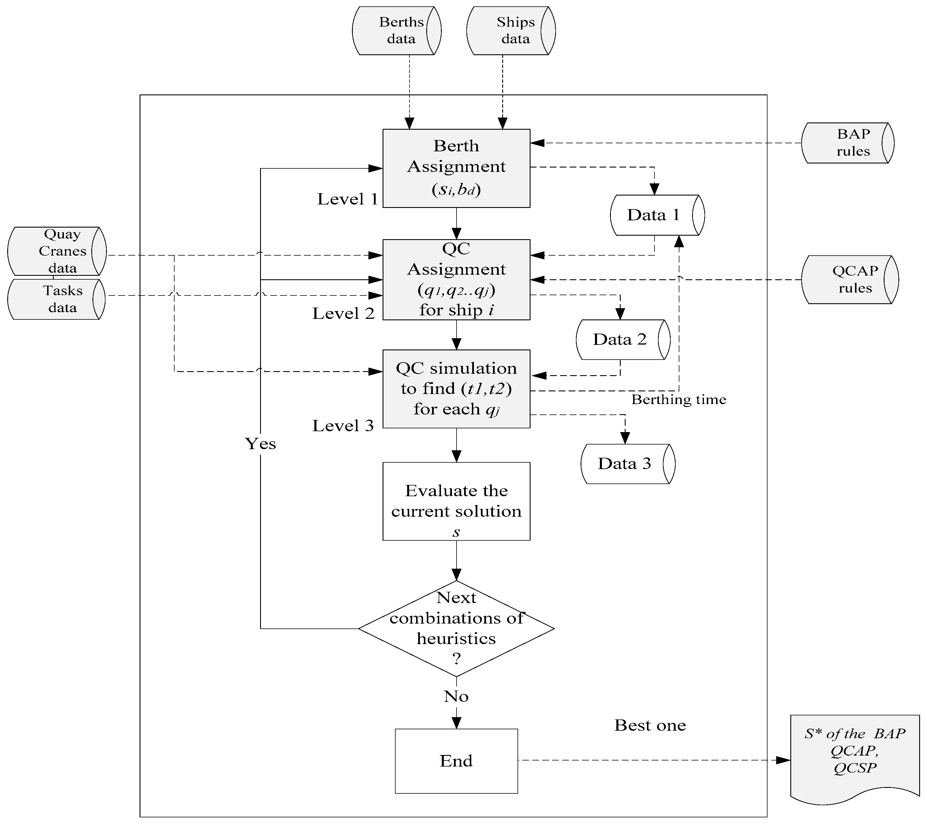
3.3. A Three-Level Framework of Planning

To solve the three problems together, a three-stage procedure is proposed as shown in Figure 1. At the first stage, each ship $i$ is assigned to a specific berth $j$ taking both constraints (2) and (3) into account. Such an assignment is denoted as (i,j) so that the decision variable $X_{ij}^t=$ 1. At the second stage, for a berth j a number of QCs are assigned to serve the ships berthing on it. For each task k of ship i, a specific quay crane q is assigned to handle it with both constraints (5) and (6) taken into consideration. This assignment is denoted as (i,q,k) and it makes the decision variable $Y_{iqk}^t=1$. At the third stage, it determines the beginning time ($T{1}_{iqk}$) and the end time ($T{2}_{iqk}$) for a task k of ship i with this schedule denoted as $\left(T{1}_{iqk},T{2}_{iqk}\right)$ that is subject to constraints (7)–(9). In Bierwirth and Meisel (2010), the authors pointed out that one way to integrate the seaside operational problems is to feed back the beginning time and completion time of the tasks determined in the QCSP to the BAP. This approach is adopted in this framework.

Each level in the framework is detailed as follows:

Level 1:

this level deals with the BAP. In this stage, heuristic rules can be used to allocate ships to berths. For example, the least workload (LWL) rule always assigns a ship to a berth that currently has the least workload. As a result, the workload among berths are balanced. The algorithm of the LWL is detailed below.

Step 1.

Set the current workload of each berth to zero.

Step 2.

Sort the calling ships by their Estimated Time of Arrivals (ETAs) to an ascending list S.

Step 3.

Sort the berths by their workloads to an ascending set B.

Step 4.

If S ≠ ∅ then

• Assign the first ship in S to the first berth in B
• Remove the first ship from S
• Go to Step 5

Else

• Go to Step 6

End if.

Step 5.

Update the current workload of the selected berth, and then go to Step 3.

Step 6.

End

Level 2:

this level deals with QCAP and QCSP. In this level, heuristics rules are used to assign QCs to ships. For example, the Load Balance (LB) rule assigns QCs to berths according to the workloads of ships assigned to berths. After determining the number of QCs assigned to each berth, the QCs are sequentially assigned to berths according to the QC number (Assume that QC along the quayside are assigned with an increasing QC number). Then, each task of a ship can be assigned to an assigned QC to that ship by using a LB rule, subjecting to the non-crossing characteristic of QCs. The LB rule is detailed below.

Step 1.

Calculate the numbers of QCs ($l_j$, $j\in B$) to be assigned to each berth j using Equation (13), in which the round operator rounds each $l_j$ off to the nearest whole digit; $N_k^i$ is the total number of containers to be handled for the task k of ship i; $n_j$ is the number of ships assigned to berth j at Level 1.

$$l_j=round\left({{\displaystyle \sum }}_{i=1}^{n_j}{\displaystyle \sum }_{k=1}^{K_i}{N}_k^i/{\displaystyle \sum }_{i=1}^m{\displaystyle \sum }_{k=1}^{K_i}{N}_k^i\right)\forall j\in B$$

(13)

Step 2.

Set the workload of each QC q to zero (i.e., $W_q=0$, q $\in Q$). And, set u = 1 and i = 1.

Step 3.

Sort all QCs into an ascending set Q = {$1,\dots ,l$} according to their QC numbers.

Step 4.

Allocate QCs one by one to each berth $j$ according to the QC numbers until the amount $l_j$ is reached. Then the QCs assigned to a same berth are a group and denoted as $Q_j$, where $j\in B$.

Step 5.

Sort the tasks of each ship i into an ascending task set $T_i$ according to the task numbers.

Step 6.

Calculate the current workload of ship i ($N_{L,uL}^i$) by totaling the numbers of containers to load ($N_L^i)$ and unload ($N_{uL}^i)$ for each task k in the task set $T_i$ using Equation (14).

$$N_{L,uL}^i=\left(N_L^i+N_{uL}^i\right)={{\displaystyle \sum }}_{k=u}^{K_i}{N}_k^i$$

(14)

Step 7.

Calculate the average number of containers ($A{N}_{L,uL}^i$) as a benchmark using Equation (15).

$$A{N}_{L,uL}^i={{\displaystyle \sum }}_{k=u}^{K_i}{N}_k^i/l_j$$

(15)

Step 8.

Calculate the respective workload of the first task k (denoted as $N_k^i$) and the second task k + 1 (denoted as $N_{k+1}^i$) in the task set Ti by totaling the number of containers to load and unload.

Step 9.

Estimate the expected workload ($W_q)$ of the first QC $q$ in $Q_j$ if the task k of ship i is added using Equation (16).

$$W_q=W_q+N_k^i$$

(16)

Step 10.

If $W_q\ge A{N}_{L,uL}^i$ then

• assign the task k of ship i to the QC q
• pop the task k out of the $T_i$
• pop the QC q out of the $Q_j$
• q = q + 1 (change to the next QC)
• $l_j=l_j-1$

Else if $W_q<A{N}_{L,uL}^i$ and $(W_q+N_{k+1}^i$) $-A{N}_{L,uL}^i\ge A{N}_{L,uL}^i-W_q$

• assign the task k of ship i to the QC q
• pop the task k out of the task set $T_i$
• pop the QC q out of the $Q_j$
• q = q + 1 (change to the next QC)
• $l_j=l_j-1$

Else

• assign the task k of ship i to the QC q
• pop the task k out of the task set $T_i$

End if

Step 11.

If $T_i\ne \varnothing$ then

• k = k + 1 (change to the next task)
• u = u + 1
• Go to Step 6

Else

• i = i + 1 (change to the next ship)
• Go to Step 12

End if

Step 12.

If $i>m$ then

• Go to Step 13

Else

• u = 1
• Go to Step 5

End if

Step 13.

End

Level 3:

this level deals with the QCSP. After determining which task is handled by which QC in level 2, this level uses a discrete simulation approach to simulate container loading and unloading for each task of a ship. As a result, the beginning and ending times of each task can be determined. Finally, the starting and ending working time of a ship are fed back to level 1 as the berthing time of each ship. The following steps are used in this level.

Step 1.

Find the task token with least available time.

Step 2.

Find the QC assigned to the task token.

Step 3.

Determine the beginning time and the end time of the task based on the available time of the assigned QC.

Step 4.

Update the available time of the QC after serving this task token.

Step 5.

Return the assigned QC.

Figure 1 also shows the data flows (dotted lines) of each level in the framework. For Level 1, the berth data, ship data, and BAP rules are inputs while Data 1 {(${\bigcup }_{i=1}^{i=m}\left(i,j\right)$: $X_{ij}^t=1$)} is an output. For Level 2, Data 1 {(${\bigcup }_{i=1}^{i=m}\left(i,j\right)$: $X_{ij}^t=1$)}, QC data, task data, and QCAP rules are inputs while Data 2 $\{{\bigcup }_{i=1}^{i=m}\left(i,q,k\right):Y_{iqk}^t=1,q\in Q,k\in K_i, t\in T$} is an output. For Level 3, the QC data, task data, and Data 2 $\{{\bigcup }_{i=1}^{i=m}\left(i,q,k\right):Y_{iqk}^t=1,q\in Q,k\in K_i, t\in T\}$ are inputs while Data 3 ($\{{\bigcup }_{i=1}^{i=m}\left(T{1}_{iqk},T{2}_{iqk}\right):Y_{iqk}^t=1,i\in S, q\in Q, q\in Q,k\in K_i, t\in T\}$) is an output. Having explored all the combinations of BAP and QCAP rules, the best solution can be found. These data are required to run the model established in the next section.

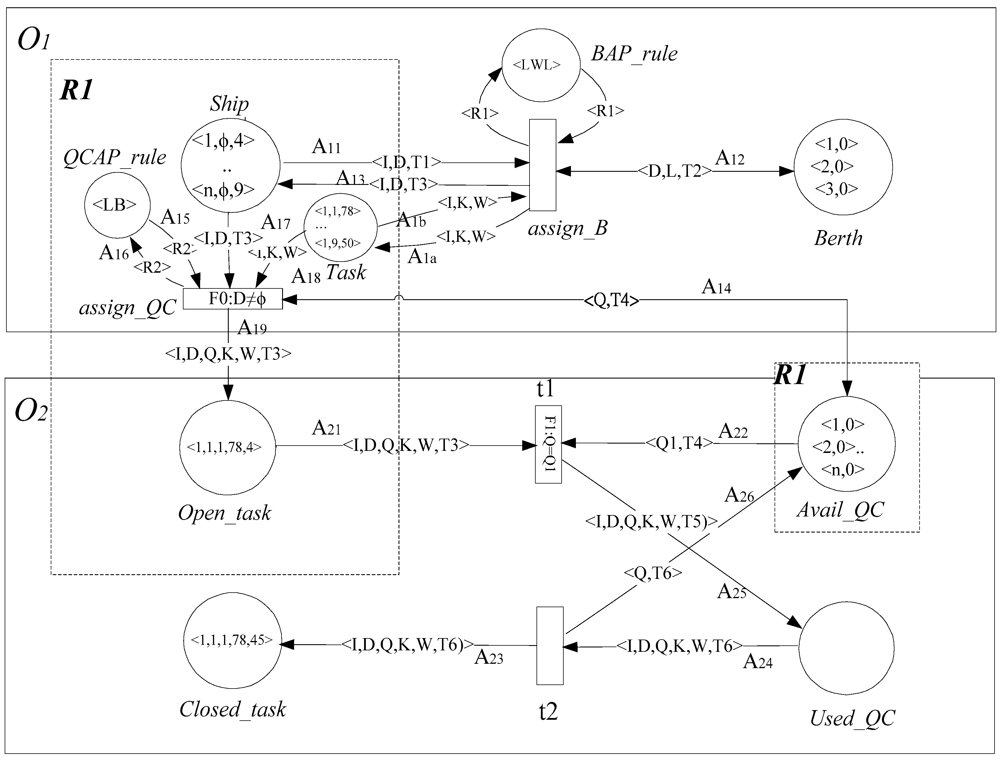
4. Modeling and Implementing the Three-Level Framework of Heuristics and Simulation

We intend to deal with the three-level planning framework using a graphical tool. For this purpose, we first define a novel high-level Petri net, termed OOTPr/Tr net, as a modeling tool. Then, based on the OOTPr/Tr net model, a program was developed using the Prolog programming language. Finally, the OOTPr/Tr net model was implemented as an evaluation tool for solving the three seaside operational problems at the same time.

4.1. The Definition of Object-Oriented and Timed Predicate/Transition Net

Definition 5.

A Timed Pr/Tr net (TPr/Tr net) is defined as 8-tuple.

TPr/Tr net = (P,T,A,Σ,L,LF,M,F,f)

where

$P$	a set of predicates. $P=P_{time}\cup P_{nontime}$, $P_i\in P_{time}$ or ${\mathrm{P}}_{nontime}$. $P_{time}\cap P_{nontime}=\varnothing$, $P_{time}$ is the set of timed predicates while $P_{nontime}$ is the set of predicates with zero time
T	a set of transitions (with logical formulas)
A	a set of arcs
Σ	a structure Σ consisting of some sort of individual tokens together with some operations (OPj) and relations (Rk), i.e., Σ = (T1,...,Ti; OP1,...,OPj; R1,...,Rk)
L	a labeling of all arcs with a formal sum of n attributes of the token’s variables (attributes), including zero-attributes that indicate a no-argument token
LF	a set of inscriptions on some transitions being logical formulas built from the operations and relations of the structure Σ; Variables occurring free in a formula have to occur at an adjacent arc
M	a marking M of the predicates of P with formal sums of n-topples of individual tokens.
F	firing rule of each element of T representing a class of possible changes of markings. Such a change, also called transition firing, consists of removing tokens from a subset of predicates and adding them to other subsets of predicates according to the expressions labeling the arcs. A transition is enabled whenever a set of tokens associated with that transition are satisfied.
$f$	$f\left(P_i\right)\to T_i$; is a function mapping $P_i$ to a handling time $T_i$; $T_i\mathrm{equals}0if{P}_i\in P_{nontime};T_i\mathrm{is}\mathrm{equal}\mathrm{to}\mathrm{or}\mathrm{greater}\mathrm{than}0\mathrm{if}{P}_i\in P_{time}$.

Definition 6.

An Object-Oriented Timed Pr/Tr net (OOTPr/Tr net) is defined as a 2-tuple:

OOTPr/Tr net = (O,R)

where

• O: is a set of finite subnet objects.
• R: is a set of communication relations between O_i.

Definition 7.

A subnet object is a TPr/Tr net with its structure defined in Definition 6.

$$O_i=\left(P,T,A,\Sigma ,L,F,f,M\right)$$

Instead of focusing on what rules are to be executed, an Object-Oriented model pays more attention to the structure, sub-models, and the communications between subnets. In an OOTPr/Tr net, subnets establish communications through predicates. If $P_i\cap P_j\ne \varnothing$ (where $P_i\in$ $O_i$ and $P_j\in O_j$) then the two subnet objects $O_i$ and $O_j$ have communication. Formed by subnet objects, an OOTPr/Tr is more readable and maintainable than a traditional TPr/Tr net.

4.2. The OOTPr/Tr Net Model for the Three-Level Framework

The OOTPr/Tr net for the three-level framework of heuristics and simulation is defined as follows.

OOTPr/Tr net = ({O₁,O₂},{R₁})

Figure 2 shows the OOTPr/Tr net model. It includes two subnets O₁ and O₂ and there is a communication relation (R₁) formed by two sets of predicates, {Task, Ship, OCAP_rule} $\in O_1$ and {Open_task, Avail_QC} $\in O_2$. When these predicates contain tokens simultaneously, it enables the transition assign_QC.

The OOTr/Pr works in this way. First, in O₁, when Ship_token <I,D,T1>, Berth_token <D,T2>, BAP_rule_token <R1>, and Task_tokens <I,K,W> respectively appear at the predicates Ship, Berth, BAR_rule, and Task at the same time, it enables the transition assign_B. After firing the transition assign_B, a BAP heuristic rule (such as LWL) will be used to assign a berth number to a ship_token <I,D,T3> with the number binding with the token variable D. For instance, if Berth 1 is assigned to the ship_token <1,D,T3> then it results in the unified Ship_token <1,1,T3>. The procedure of binding a value with a token variable is called “unification”, which leads to the generation of a unified token. This assignment, indicated as (i,j) = (1,1) or $X_{11}^t$ = 1, will be part of the solution to the BAP. After this, a unified token will return to the predicate Ship and it will trigger the subnet O₁ to check the existence of the following tokens: QCAP_rule_token <LB>, Task_tokens <I,K,W> and Avail_QC_tokens <Q,T4>. If these tokens respectively appear at the predicates, Ship, QCAP_rule, Task, and Avail_QC, respectively, and meanwhile the logical formula F0 (D ≠ $\varnothing$) is satisfied, the transition assign_QC will be enabled. After firing the transition assign_QC, a QCAP rule will assign an Avail_QC_token <Q,T4> to a Task_token <I,K,W>. For instance, if the Avail_QC_token <1,0> is assigned to the Task_token <1,1,78> it then generates a Open_task_token <1,1,Q,1,78,T3> in which the token variable Q is bound with the value 1 and the token variable T3 will be unified with the value Max{T1,T2,T4} = max{4,0,0} = 4. This assignment, indicated as (i,q,k) = (1,1,1) or $Y_{111}^t=1$, will be part of the solution to the QCAP.

In O₂, it will start simulating the loading and unloading of containers. When the tokens Open_Task_tokens <1,1,1,1,78,4> and Avail_QC_tokens <1,0> simultaneously appear at the corresponding predicate Open_task and Avail_QC, respectively, with the logical formula F1 (Q = Q1) also being satisfied, it enables the transition t1. After firing the transition t1, it will generate a begin_event, E(t1,I,Q,K), and transform the Open_task_token <1,1,1,1,78,4> into a used_QC_token <1,1,1,1,78,T5> to stay at the predicate Used_QC. The event time t1 and token variable T5 will bind with the value Max{T3,T4} = Max{4,0} = 4. After the firing of t2, it generates an end_event, denoted as E(t2,I,Q,K). The T6 will unify with the value, T5+usage_time. After this, the used_ QC_token <1,T6> will return to the predicate Avail_QC as a Avail_QC_token <1,T6> and meanwhile a Closed_Task_token <1,1,1,1,78,T6> will be generated and transited to the predicate Close_task. Then [$T{1}_{111}$,$T{2}_{111}]$ = [4,T6] is generated as a partial schedule of QC 1.

While there are still other Open_task_tokens <I,D,Q,K,W,T3> at the predicate Open_task another simulation run will be generated; Otherwise, if all Open_task_tokens <I,D,Q,K,W,T3> have been transited to the predicate Closed_task then the simulation stops running. When there are other BAP_rule_tokens and/or QCAP_rule_tokens at the predicates BAP_rule and/or QCAP_rule, respectively, it will continue to trigger more simulation runs to explore alternative solutions based on the combinations of the two kinds of heuristic rules. The best solution will be finally identified. We regard this graphical model as a discrete event simulation model.

4.3. The Algorithm for Implementing the OOTPr/Tr Net Model

Based on the proposed OOTPr/Tr net model, the algorithm with detailed steps to derive all solutions to the three seaside operational problems is outlined as follows:

Step 1	Place the Ship_token <I,D,T1>, Berth_token <D,L,T2>, BAP_rule_token <R1>, QCAP_rule_token <R2>, Task_token <I,D,W>, Avail_QC_token <Q1,T4> at the predicates Ship, Berth, BAR_rule, QCAP_rule, Task, and Avail_QC, respectively.
Step 2	(In O1) trigger the transition assign_B, it will assign a berth_token <D,L,T2> to the Ship_token <I,D,T1> using a BAP_rule_token <R1>.
Step 3	Trigger the transition assign_QC, it will assign a number of QCs to each berth (D) using the QCAP_rule_token <R2>. In addition, a QC (Q) will be subsequently assigned to handle a specific Open_Task_token <I,D,Q,K,W,T3> of the specific ship I.
Step 4	(In O2) trigger the transition t1, it will simulate loading and unloading Open_Task_tokens <I,D,Q,K,W,T3> based on assigned QCs. Repeat this until all Open_Task_tokens <I,D,Q,K,W,T3> have been completed and transited to the predicate Close_task as Close_task_tokens <I,D,Q,K,W,T6>. During the simulation, generate the beginning time ($T{1}_{iqk})$ and the end time ($T{2}_{iqk})$ for each task of a ship. This results in a solution s.
Step 5	Evaluate the solution s using the objective function defined in Equation (1).
Step 6	Compare the solution s to the current best solution s*. If s > s* then s* = s.
Step 7	Check whether there are other BAP_rule_token <R1> and/or QCAP_rule_token <R2>. If “yes” then go to Step 1; Otherwise, go to Step 8.
Step 8	Determine the berthing time (BTi) of each ship i using Equation (10).
Step 9	End

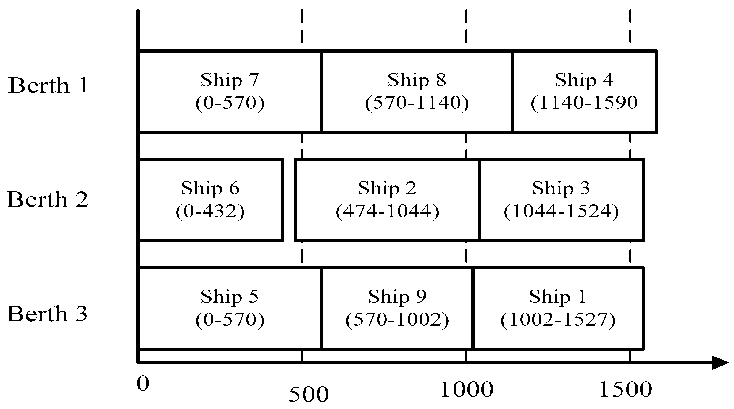
5. Numerical Example

Hsu and Su [42] and Hsu and Hsu [43] have proposed a systematic procedure for the implementation of a Pr/Tr net model. Accordingly, we have implemented the OOTPr/Tr net model as an evaluation tool using the Prolog programming language. Using the input data as described in Section 5.1, the derived output data are shown in Section 5.2.

5.1. Inputs

To run the OOTPr/Tr net, relevant inputs such as berths, ships, QCs, tasks, BAP rules, and QCAP rules are required. The Appendix A lists all the input data for this example in which 9 ships, 3 berths, 10 QCs, and some tasks of calling ships are included.

5.2. Outputs

After running the simulation tool,

Table 1. The total solution to BAP, QCAP, and QCSP

j	${\mathit{Y}}_{\mathit{i}\mathit{q}\mathit{k}}^{\mathit{t}}$ = 1			$\mathit{T}{1}_{\mathit{i}\mathit{q}\mathit{k}}$	$\mathit{T}{2}_{\mathit{i}\mathit{q}\mathit{k}}$	Duration
	q	i	k
1	1	ship 7	1	0	174	174
1	1	ship 7	5	174	339	165
1	2	ship 7	7	0	282	282
1	3	ship 7	9	0	240	240
1	3	ship 7	11	240	390	150
1	3	ship 7	13	390	570	180
1	1	ship 8	1	570	744	174
1	1	ship 8	5	744	909	165
1	2	ship 8	7	570	852	282
1	3	ship 8	9	570	810	240
1	3	ship 8	11	810	960	150
1	3	ship 8	13	960	1140	180
1	1	ship 4	1	1140	1440	300
1	2	ship 4	3	1140	1374	234
1	2	ship 4	5	1374	1539	165
1	3	ship 4	7	1140	1305	165
1	3	ship 4	9	1305	1590	285
2	4	ship 6	5	0	132	132
2	4	ship 6	7	132	417	285
2	5	ship 6	9	0	189	189
2	5	ship 6	11	189	474	285
2	6	ship 6	13	0	147	147
2	6	ship 6	15	147	432	285
2	4	ship 2	3	474	699	225
2	4	ship 2	5	699	954	255
2	5	ship 2	7	474	699	225
2	5	ship 2	9	699	996	297
2	6	ship 2	11	474	759	285
2	6	ship 2	15	759	1044	285
2	4	ship 3	1	1044	1215	171
2	4	ship 3	3	1215	1440	225
2	4	ship 3	5	1440	1650	210
2	5	ship 3	7	1044	1314	270
2	5	ship 3	9	1314	1584	270
2	6	ship 3	11	1044	1329	285
2	6	ship 3	13	1329	1524	195
3	7	ship 5	1	0	255	255
3	7	ship 5	5	255	540	285
3	8	ship 5	7	0	282	282
3	8	ship 5	9	282	567	285
3	9	ship 5	11	0	249	249
3	9	ship 5	13	249	570	321
3	10	ship 5	15	0	285	285
3	7	ship 9	5	570	702	132
3	7	ship 9	7	702	987	285
3	8	ship 9	9	570	759	189
3	9	ship 9	11	570	855	285
3	10	ship 9	13	570	717	147
3	10	ship 9	15	717	1002	285
3	7	ship 1	1	1002	1212	210
3	7	ship 1	3	1212	1497	285
3	8	ship 1	5	1002	1167	165
3	8	ship 1	7	1167	1392	225
3	9	ship 1	9	1002	1296	294
3	9	ship 1	11	1296	1581	285
3	10	ship 1	13	1002	1242	240
3	10	ship 1	15	1242	1527	285

j: berth id; q: QC id; i: ship id; k: task id; $T{1}_{iqk}$: begin time; $T{2}_{iqk}$: end time.

shows the total solution to the BAP, QCAP, and QCSP. For ship 7, it is assigned to berth 1 and QC 1 is assigned to handle tasks 1 and 5; QC 2 handles the task 7; and QC 3 handles tasks 11 and 13. For each task k, a QC q is assigned to work it during the time period [$T{1}_{iqk}$, $T{2}_{iqk}$]. For instance, the QC 1 is assigned to handle task 1 of ship 7 during the time period [0,174].

Table 2. The schedule of QCs (sorted by QC No.).

j	${\mathit{Y}}_{\mathit{i}\mathit{q}\mathit{k}}^{\mathit{t}}=1$			$\mathit{T}{1}_{\mathit{i}\mathit{q}\mathit{k}}$	$\mathit{T}{2}_{\mathit{i}\mathit{q}\mathit{k}}$	Duration
	q	i	k
1	1	ship 7	1	0	174	174
1	1	ship 7	5	174	339	165
1	1	ship 8	1	570	744	174
1	1	ship 8	5	744	909	165
1	1	ship 4	1	1140	1440	300
1	2	ship 7	7	0	282	282
1	2	ship 8	7	570	852	282
1	2	ship 4	3	1140	1374	234
1	2	ship 4	5	1374	1539	165
1	3	ship 7	9	0	240	240
1	3	ship 7	11	240	390	150
1	3	ship 7	13	390	570	180
1	3	ship 8	9	570	810	240
1	3	ship 8	11	810	960	150
1	3	ship 8	13	960	1140	180
1	3	ship 4	7	1140	1305	165
1	3	ship 4	9	1305	1590	285
2	4	ship 6	5	0	132	132
2	4	ship 6	7	132	417	285
2	4	ship 2	3	474	699	225
2	4	ship 2	5	699	954	255
2	4	ship 3	1	1044	1215	171
2	4	ship 3	3	1215	1440	225
2	4	ship 3	5	1440	1650	210
2	5	ship 6	9	0	189	189
2	5	ship 6	11	189	474	285
2	5	ship 2	7	474	699	225
2	5	ship 2	9	699	996	297
2	5	ship 3	7	1044	1314	270
2	5	ship 3	9	1314	1584	270
2	6	ship 6	13	0	147	147
2	6	ship 6	15	147	432	285
2	6	ship 2	11	474	759	285
2	6	ship 2	15	759	1044	285
2	6	ship 3	11	1044	1329	285
2	6	ship 3	13	1329	1524	195
3	7	ship 5	1	0	255	255
3	7	ship 5	5	255	540	285
3	7	ship 9	5	570	702	132
3	7	ship 9	7	702	987	285
3	7	ship 1	1	1002	1212	210
3	7	ship 1	3	1212	1497	285
3	8	ship 5	7	0	282	282
3	8	ship 5	9	282	567	285
3	8	ship 9	9	570	759	189
3	8	ship 1	5	1002	1167	165
3	8	ship 1	7	1167	1392	225
3	9	ship 5	11	0	249	249
3	9	ship 5	13	249	570	321
3	9	ship 9	11	570	855	285
3	9	ship 1	9	1002	1296	294
3	9	ship 1	11	1296	1581	285
3	10	ship 5	15	0	285	285
3	10	ship 9	13	570	717	147
3	10	ship 9	15	717	1002	285
3	10	ship 1	13	1002	1242	240
3	10	ship 1	15	1242	1527	285

j: berth id; q: QC id; i: ship id; k: task id; $T{1}_{iqk}$: begin time; $T{2}_{iqk}$: end time.

shows the schedules for all QCs. The solution to the BAP is denoted as

$$\{{\bigcup }_{i=1}^m\left(i,j\right):X_{ij}^t=1\}=\{\left(1,3\right),\left(2,2\right),\left(3,2\right),\left(4,1\right),\left(5,3\right),\left(6,2\right),\left(7,1\right),\left(8,1\right),\left(9,3\right)\}$$

Furthermore, based on Equation (10), the BT₁ to BT₉ of the calling ships are derived as follows.

BT₁ = [1002,1757]

BT₂ = [474,1044]

BT₃ = [1044,1524]

BT₄ = [1140,1590]

BT₅ = [0,570]

BT₆ = [0,432]

BT₇ = [0,570]

BT₈ = [570,1140]

BT₉ = [570,1002]

Figure 3 shows the berthing plan for these calling ships. The total makespan of this berthing plan is 1590, and is found to be quite promising as the workloads on these berths are well balanced. As a result, the makespan on Berth 1 (1590) is very close to the makespan on Berth 2 (1524) as well as the makespan on Berth 3 (1527). In addition, it is found that the berth utilization rates for Berth 1, Berth 2, and Berth 3 reach 100%, 97%, and 100%, respectively, which indicates that these scarce resources can be efficiently utilized.

6. Conclusions and Future Research Direction

To deal with increasing shipments of containers, improving the efficiency of a container terminal is important. To achieve this, one effective way is to directly improve the operational efficiency of a CT. As most past studies were found to have solved the three seaside operational problems separately, which tends to result in poor overall system performance, solving the three seaside operational problems together is thus necessary. Therefore, in this research we have employed a graphical tool, termed an OOTPr/Tr net, to model and solve them at the same time.

Due to the search in a reduced solution space, one advantage of our approach is that it can avoid the computationally intractable problems often encountered by exact approaches when they are used to deal with problems of practical size. Another advantage of our approach is that it can avoid the problems of being time-consuming and labor-intensive that are faced by “what-if” analyses in a traditional simulation approach. In our approach, after giving formal definitions to the three seaside operational problems, we transformed them into a three-level framework. This framework was then further modeled by a novel graphical tool, the OOTPr/Tr net. Finally, we implemented this OOTPr/Tr net as an evaluation tool using the Prolog programming language. Our experimental results showed the applicability of this tool. The contributions of this research are highlighted as follows.

(1)

We have initiated a novel graphical tool, termed OOTPr/Tr net, which can be used for modeling and problem solving.

(2)

Using this novel graphical tool, we have successfully modeling the three seaside operational problems. This model was found to be quite flexible since resources such as ships, berths, and QCs are represented as tokens that can easily added into the model. In addition, we have implemented the derived OOTPr/Tr net as an evaluation tool.

(3)

The approach proposed in this study can be regarded as a simulation approach based on a reduced search space formed by the combinations of BAP and QCAP heuristic rules.

As this research has only studied a few combinations of the various heuristic rules, future research can investigate the results obtained from other heuristic rules. In addition, one can treat the arrival times and processing times as uncertain factors to take uncertainty into consideration.

References

1. Chung, S.H.; Choy, K.L. A modified genetic algorithm for quay crane scheduling operations. Expert Syst. Appl. 2012, 39, 4213–4221. [Google Scholar] [CrossRef]
2. Salido, M.A.; Mario, R.M.; Barber, E. A decision support system for managing combinatorial problems in a container terminal. Knowl. Based Syst. 2012, 29, 63–74. [Google Scholar] [CrossRef]
3. Liu, Y.B.; Zhou, C.G.; Guo, D.G.; Wang, K.P.; Pang, W.P.; Zhai, Y.K. A decision support system using soft computing for modern international container transportation services. Appl. Soft Comput. 2012, 10, 1087–1095. [Google Scholar] [CrossRef]
4. Vis, I.F.A.; de Koster, R. Transshipment of container at a container terminal: An overview. Eur. J. Oper. Res. 2003, 147, 1–16. [Google Scholar] [CrossRef]
5. Bierwirth, C.; Meisel, F. A survey of berth allocation and quay crane scheduling problems in container terminals. Eur. J. Oper. Res. 2010, 202, 615–627. [Google Scholar] [CrossRef]
6. Lee, Y.; Chen, C.Y. An optimization heuristic for the berth scheduling problem. Eur. J. Oper. Res. 2009, 196, 500–508. [Google Scholar] [CrossRef]
7. Liang, C.J.; Huang, Y.F.; Yang, Y. A quay crane dynamic scheduling problem by hybrid evolutionary algorithm for berth allocation planning. Comput. Ind. Eng. 2009, 56, 1021–1028. [Google Scholar] [CrossRef]
8. Raa, B.; Dullaert, W.; Schaeren, R.V. An enriched model for the integrated berth allocation and quay crane assignment problem. Expert Syst. Appl. 2011, 38, 14136–14147. [Google Scholar] [CrossRef]
9. Zhang, C.R.; Zheng, L.; Zhang, Z.H.; Shi, L.Y.; Armstrong, A.J. The allocation of berths and quay cranes by using a sub-gradient optimization technique. Comput. Ind. Eng. 2010, 58, 40–50. [Google Scholar] [CrossRef]
10. Lee, D.H.; Wang, H.Q.; Miao, L. Quay crane scheduling with handling priority in port container terminals. Eng. Optim. 2008, 40, 179–189. [Google Scholar] [CrossRef]
11. Canonaco, P.; Legato, P.; Mazza, R.M.; Musmanno, R. A queuing network model for the management of berth crane operations. Comput. Oper. Res. 2008, 35, 2432–2446. [Google Scholar] [CrossRef]
12. Kim, K.H.; Park, Y.M. A crane scheduling method for port container terminals. Eur. J. Oper. Res. 2004, 156, 752–768. [Google Scholar] [CrossRef]
13. Zhang, H.; Kim, K.H. Maximizing the number of dual-cycle operations of quay cranes in container terminals. Comput. Ind. Eng. 2009, 56, 979–992. [Google Scholar] [CrossRef]
14. Legato, P.; Mazza, R.M. Berth planning and resource optimization at container terminal via discrete event simulation. Eur. J. Oper. Res. 2001, 133, 537–547. [Google Scholar] [CrossRef]
15. Peterkofsky, R.I.; Daganzo, C.R. A branch and bound solution method for the crane scheduling problem. Transp. Res. B 1990, 24, 159–172. [Google Scholar] [CrossRef]
16. Sun, Z.; Lee, L.H.; Chew, E.P.; Tan, K. MicroPort: A general simulation platform for seaport container terminals. Adv. Eng. Inform. 2012, 26, 80–89. [Google Scholar] [CrossRef]
17. Liang, C.J.; Guo, J.Q.; Yang, Y. Multi-objective hybrid genetic algorithm for quay crane dynamic assignment in birth allocation planning. J. Intell. Manuf. 2011, 22, 471–479. [Google Scholar] [CrossRef]
18. Jin, Z.H.; Li, N. Optimization of quay crane dynamic scheduling based on berth schedules in container terminal. J. Transp. Syst. Eng. Inf. Technol. 2011, 1, 58–64. [Google Scholar] [CrossRef]
19. Imai, A.; Chen, H.C.; Nishimura, E.; Papadimitriou, S. The simultaneous berth and quay crane allocation problem. Transp. Res. E 2008, 44, 900–920. [Google Scholar] [CrossRef]
20. Zhou, P.R.; Kang, H.G. Study on berth and quay-crane allocation under stochastic environments in container terminal. Syst. Eng. Theory Pract. 2008, 28, 161–169. [Google Scholar] [CrossRef]
21. Chang, D.F.; Jiang, Z.H.; Yan, W.; He, J.L. Integrating berth allocation and quay crane assignments. Transp. Res. E 2010, 46, 975–990. [Google Scholar] [CrossRef]
22. Lee, D.H.; Wang, H.Q. Integrated discrete berth allocation and quay crane scheduling in port container terminals. Eng. Optim. 2010, 42, 747–761. [Google Scholar] [CrossRef]
23. Han, X.L.; Lu, Z.Q.; Xi, L.R. A proactive approach for simultaneous berth and quay crane scheduling problem with stochastic arrival and handling time. Eur. J. Oper. Res. 2010, 207, 1327–1340. [Google Scholar] [CrossRef]
24. Xu, D.S.; Li, C.L.; Leung, J.Y.T. Berth allocation with time-dependent physical limitations on vessels. Eur. J. Oper. Res. 2012, 216, 47–56. [Google Scholar] [CrossRef]
25. Ng, W.C.; Mak, K.L. Quay crane scheduling in container terminals. Eng. Optim. 2006, 38, 723–737. [Google Scholar] [CrossRef]
26. Legato, P.; Trunfio, R.; Meisel, F. Modeling and solving rich quay crane scheduling problems. Comput. Oper. Res. 2012, 39, 2063–2078. [Google Scholar] [CrossRef]
27. Maione, G.; Mangini, A.M.; Ottomanelli, M. A Generalized Stochastic Petri Net Approach for Modeling Activities of Human Operators in Intermodal Container Terminals. IEEE Trans. Autom. Sci. Eng. 2016, 13, 1504–1516. [Google Scholar] [CrossRef]
28. Zhang, F.A.H.; Jiang, S.B.Z. Modeling and Analysis of Container Terminal Logistics System by Extended Generalized Stochastic Petri Nets. In Proceedings of the 2006 IEEE International Conference on Service Operations and Logistics, and Informatics, Shanghai, China, 21–23 June 2006; pp. 310–315.
29. Murty, K.G.; Liu, J.Y.; Wan, Y.W.; Linn, R. A decision support system for operations in a container terminal. Decis. Support Syst. 2005, 59, 309–332. [Google Scholar] [CrossRef]
30. Song, L.I.; Cherrett, T.; Guan, W. Study on berth planning problem in a container seaport: Using an integrated programming approach. Comput. Ind. Eng. 2012, 62, 119–128. [Google Scholar] [CrossRef]
31. Wu, N.Q.; Zhou, M.C.; Li, Z.W. Short-Term Scheduling of Crude-Oil Operations: Enhancement of Crude-Oil Operations Scheduling Using a Petri Net-Based Control-Theoretic Approach. IEEE Robot. Autom. Mag. 2015, 22, 64–76. [Google Scholar] [CrossRef]
32. Yang, R.; Wu, N.; Qiao, Y.; Zhou, M.C. Petri Net-Based Polynomially Complex Approach to Optimal One-Wafer Cyclic Scheduling of Hybrid Multi-Cluster Tools in Semiconductor Manufacturing. IEEE Trans. Syst. Man Cybern. Syst. 2014, 44, 1598–1610. [Google Scholar] [CrossRef]
33. Wu, N.; Zhou, M.C. Schedulability Analysis and Optimal Scheduling of Dual-Arm Cluster Tools with Residency Time Constraint and Activity Time Variation. IEEE Trans. Autom. Sci. Eng. 2012, 9, 203–209. [Google Scholar]
34. Petering, M.E.H. Decision support for yard capacity, fleet composition, truck substitutability, and scalability issues at seaport container terminals. Transp. Res. E 2011, 47, 85–103. [Google Scholar] [CrossRef]
35. Kim, K.H.; Moon, K.C. Berth scheduling by simulated annealing. Transp. Res. B 2003, 37, 541–560. [Google Scholar] [CrossRef]
36. Wang, F.; Lim, A. A stochastic beam search for the berth allocation problem. Decis. Support Syst. 2007, 42, 2186–2196. [Google Scholar] [CrossRef]
37. Zhen, L.; Hay, L.H.; Chew, E.P. A decision model for berth allocation under uncertainty. Eur. J. Oper. Res. 2011, 212, 54–68. [Google Scholar] [CrossRef]
38. Buhrkal, K.; Zuglian, S.; Ropke, S.; Larsen, J.; Lusby, R. Models for the discrete berth allocation problem: A computational comparison. Transp. Res. E 2011, 47, 461–473. [Google Scholar] [CrossRef]
39. Yin, X.R.; Khoo, L.P.; Chen, C.H. A distributed agent system for port planning and scheduling. Adv. Eng. Inform. 2011, 25, 403–412. [Google Scholar] [CrossRef]
40. Zeng, Q.C.; Yang, Z.Z.; Lai, L.Y. Models and algorithms for multi-crane oriented scheduling method in container terminals. Transp. Policy 2009, 16, 271–278. [Google Scholar] [CrossRef]
41. Pratap, S.; Daultani, Y.; Tiwari, M.K.; Mahanty, B. Rule based optimization for a bulk handling port operations. J. Intell. Manuf. 2015, 1–25. [Google Scholar] [CrossRef]
42. Hsu, H.P.; Su, S.T. The implementation of an Activity-Based Costing collaborative production planning system for semiconductor backend production. Int. J. Prod. Res. 2005, 43, 2473–2492. [Google Scholar] [CrossRef]
43. Hsu, H.P.; Hsu, H.M. Systematic modeling and implementation of a resource planning system for virtual enterprise by Predicate/Transition net. Expert Syst. Appl. 2008, 35, 1841–1857. [Google Scholar] [CrossRef]
Figure 1. The input and output of the three-level framework of heuristics for simulation. Data 1: the { i = 1 i = m ( i , j ) } ; Data 2: { i = 1 i = m ( i , q , k ) } ; Data 3: { i = 1 i = m ( T 1 i q k , T 2 i q k ) } .
Applsci 07 00218 g001
Figure 2. The OOTPr/Tr net model for the three-level framework.
Applsci 07 00218 g002
Figure 3. The berthing planning for 9 calling ships.
Applsci 07 00218 g003