Existence, Stability and Dynamics of Nonlinear Modes in a 2D PartiallyPT Symmetric Potential

Abstract

It is known that multidimensional complex potentials obeying parity-time ($\mathcal{PT}$) symmetry may possess all real spectra and continuous families of solitons. Recently, it was shown that for multi-dimensional systems, these features can persist when the parity symmetry condition is relaxed so that the potential is invariant under reflection in only a single spatial direction. We examine the existence, stability and dynamical properties of localized modes within the cubic nonlinear Schrödinger equation in such a scenario of partially $\mathcal{PT}$-symmetric potential.

1. Introduction

The study of $\mathcal{PT}$ (parity–time) symmetric systems was initiated through the works of Bender and collaborators [1,2]. Originally, it was proposed as an alternative to the standard quantum theory, where the Hamiltonian is postulated to be Hermitian. In these works, it was instead found that Hamiltonians invariant under $\mathcal{PT}$-symmetry, which are not necessarily Hermitian, may still give rise to completely real spectra. Thus, the proposal of Bender and co-authors was that these Hamiltonians are appropriate for the description of physical settings. In the important case of Schrödinger-type Hamiltonians, which include the usual kinetic-energy operator and the potential term, $V\left(x\right)$, the $\mathcal{PT}$-invariance is consonant with complex potentials, subject to the constraint that $V^{*}\left(x\right)=V(-x)$.

A decade later, it was realized (and since then it has led to a decade of particularly fruitful research efforts) that this idea can find fertile ground for its experimental realization although not in quantum mechanics where it was originally conceived. In this vein, numerous experimental realizations sprang up in the areas of linear and nonlinear optics [3,4,5,6,7,8], electronic circuits [9,10,11], and mechanical systems [12], among others. Very recently, this now mature field of research has been summarized in two comprehensive reviews [7,8].

One of the particularly relevant playgrounds for the exploration of the implications of $\mathcal{PT}$-symmetry is that of nonlinear optics, especially because it can controllably involve the interplay of $\mathcal{PT}$-symmetry and nonlinearity. The relevant efforts have gradually progressed from the simpler setting of coupled waveguides (bearing gain and loss) to entire $\mathcal{PT}$-symmetric lattices and the identification of optical solitons in them. These developments hold considerable promise for the potential realization of more complex settings, such as the one proposed herein. In this context, the propagation of light (in systems such as optical fibers or waveguides [7,8]) is modeled by the nonlinear Schrödinger equation of the form:

$$\begin{array}{c}\hfill i{\mathsf{\Psi }}_z+{\mathsf{\Psi }}_{xx}+{\mathsf{\Psi }}_{yy}+U(x,y)\mathsf{\Psi }+\sigma {\left|\mathsf{\Psi }\right|}^2\mathsf{\Psi }=0.\end{array}$$

(1)

In the optics notation that we use here, the evolution direction is denoted by z, the propagation distance. Here, we restrict our considerations to two spatial dimensions and assume that the potential $U(x,y)$ is complex valued, representing gain and loss in the optical medium, depending on the sign of the imaginary part (negative for gain, positive for loss) of the potential. In this two-dimensional setting, the condition of full $\mathcal{PT}$-symmetry in two dimensions is that $U^{*}(x,y)=U(-x,-y)$. Potentials with full $\mathcal{PT}$ symmetry have been shown to support continuous families of soliton solutions [13,14,15,16,17,18]. However, an important recent development was the fact that the condition of (full) $\mathcal{PT}$ symmetry can be relaxed. That is, either the condition $U^{*}(x,y)=U(-x,y)$ or $U^{*}(x,y)=U(x,-y)$ of, so-called, partial $\mathcal{PT}$ symmetry can be imposed, yet the system will still maintain all real spectra and continuous families of soliton solutions [19]. Other subsequent results include stable vortex structures in cubic nonlinear media under the influence of partially $\mathcal{PT}$-symmetric azimuthal potentials [20].

In the original contribution of [19], only the focusing nonlinearity case was considered for two select branches of solutions and the stability of these branches was presented for isolated parametric cases (of the frequency parameter of the solution). Our aim in the present work is to provide a considerably more “spherical” perspective of the problem. The corresponding physical scenario that we have in mind involves a medium featuring a cubic nonlinearity. Given that the potential of [19] was principally featuring four “nodes”, we are envisioning an implementation involving a four waveguide system. This is both in the spirit of the pioneering (two waveguide) work of [3] and also in that of subsequent proposals for trimers and quadrimers (i.e., three and four waveguide systems, respectively) [21,22]. A more remote possibility is that of a continuous cubic nonlinearity medium bearing a complex index of refraction in accordance with the prescription of [19], although, to the best of our understanding, such a possibility appears less tractable on the basis of current experimental capabilities.

In what follows, we examine the bifurcation of nonlinear modes from all three point spectrum eigenvalues of the underlying linear Schrödinger operator of the partially $\mathcal{PT}$-symmetric potential. Upon presenting the relevant model (Section 2), we perform the relevant continuations (Section 3) unveiling the existence of nonlinear branches both for the focusing and for the defocusing nonlinearity case. We also provide a systematic view towards the stability of the relevant modes (Section 4), by characterizing their principal unstable eigenvalues as a function of the intrinsic frequency parameter of the solution. In Section 5, we complement our existence and stability analysis by virtue of direct numerical simulations that manifest the result of the solutions’ dynamical instability when they are found to be unstable. Finally, in Section 6, we summarize our findings and present our conclusions, as well as discussing some possibilities for future studies.

2. Model, Theoretical Setup and Linear Limit

Motivated by the partially $\mathcal{PT}$-symmetric setting of [19], we consider the complex potential $U(x,y)=V(x,y)+iW(x,y)$ where

$$\begin{array}{ccc}\hfill V& =& \left(a{e}^{-{(y-y_0)}^2}+b{e}^{-{(y+y_0)}^2}\right)\left(e^{-{(x-x_0)}^2}+e^{-{(x+x_0)}^2}\right)\hfill \\ \hfill W& =& \beta \left(c{e}^{-{(y-y_0)}^2}+d{e}^{-{(y+y_0)}^2}\right)\left(e^{-{(x-x_0)}^2}-e^{-{(x+x_0)}^2}\right).\hfill \end{array}$$

(2)

with real constants β, $a\ne b$ and $c\ne -d$. The potential is chosen with partial $\mathcal{PT}$-symmetry so that $U^{*}(x,y)=U(-x,y)$. That is, the real part is even in the x-direction with $V(x,y)=V(-x,y)$ and the imaginary part is odd in the x-direction with $-W(x,y)=W(-x,y)$. The constants $a,b,c,d$ are chosen such that there is no symmetry in the y direction.

In [19], it is shown that the spectrum of the potential U can be all real as long as $\left|\beta \right|$ is below a threshold value, after which a ($\mathcal{PT}$-) phase transition occurs; this is a standard property of $\mathcal{PT}$-symmetric potentials. For the case of $a=3,b=c=2,d=1$, the spectrum is real below the threshold value of $\left|\beta \right|\approx 0.214$; we focus on $\beta =0.1$, i.e., we operate well below this critical point. 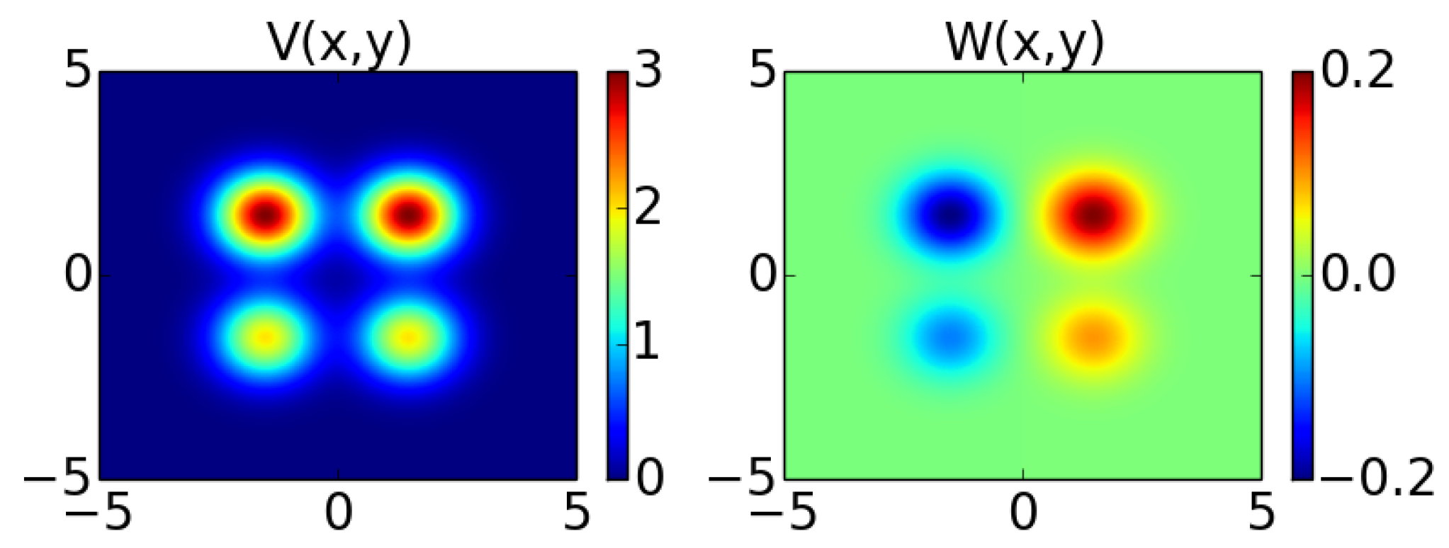Figure 1 shows plots of the potential U. The real part of the potential is shown on the left, while the imaginary part associated with gain-loss is on the right; the gain part of the potential corresponds to $W<0$ and occurs for $x<0$, while the loss part with $W>0$ occurs for $x>0$. 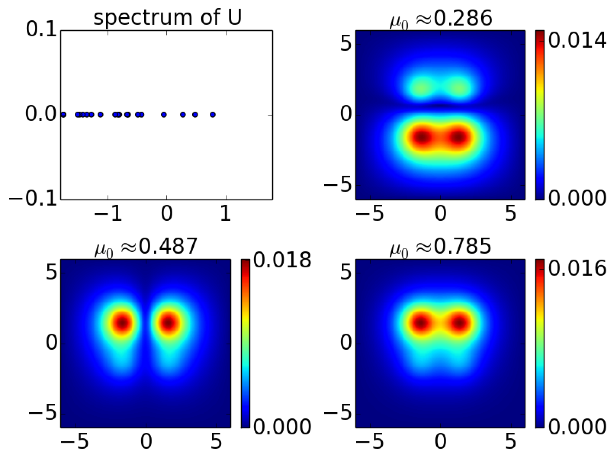Figure 2 shows the spectrum of U, i.e., eigenvalues for the underlying linear Schrödinger problem $({\nabla }^2+U){\psi }_0={\mu }_0{\psi }_0$. The figure also shows the magnitude of the corresponding eigenvectors for the three discrete real eigenvalues ${\mu }_0$. It is from these modes that we will seek bifurcations of nonlinear solutions in what follows. It is worthwhile to mention here, in comparison, e.g., with the real four-well potential of [23] that the latter possessed four localized modes, with the fourth antisymmetric, quadrupolar one being absent from the point spectrum in the case of interest herein.

3. Existence: Nonlinear Modes Bifurcating from the Linear Limit

As is customary, we focus on stationary soliton solutions of (1) of the form $\mathsf{\Psi }(x,y,z)=\psi (x,y)e^{i\mu z}$. Thus, one obtains the following stationary equation for $\psi (x,y)$.

$${\psi }_{xx}+{\psi }_{yy}+U(x,y)\psi +\sigma {\left|\psi \right|}^2\psi =\mu \psi$$

(3)

In [19], it is discussed that a continuous family of solitons bifurcates from each of the linear solutions in the presence of nonlinearity. In order to see this, let ${\mu }_0$ be a discrete simple real eigenvalue of the potential U (such as one of the positive real eigenvalues in the top left plot of Figure 2). Now, following [19], expand $\psi (x,y)$ in terms of $ϵ=|\mu -{\mu }_0|<<1$ and substitute the expression

$$\psi (x,y)={ϵ}^{1/2}\left[c_0{\psi }_0+ϵ{\psi }_1+{ϵ}^2{\psi }_2+\cdots \right]$$

(4)

into Equation (3). This gives the equation for ${\psi }_1$ as

$$L{\psi }_1=c_0\left(\rho {\psi }_0-\sigma |c_0{|}^2{\left|{\psi }_0\right|}^2{\psi }_0\right)$$

(5)

where $\rho =\mathrm{sgn}(\mu -{\mu }_0)$ and

$$|c_0{|}^2=\frac{\rho \langle {\psi }_0^{*},{\psi }_0\rangle }{\sigma \langle {\psi }_0^{*},|{\psi }_0{|}^2{\psi }_0\rangle }.$$

(6)

Here, ${\psi }_0^{*}$ plays the role of the adjoint solution to ${\psi }_0$.

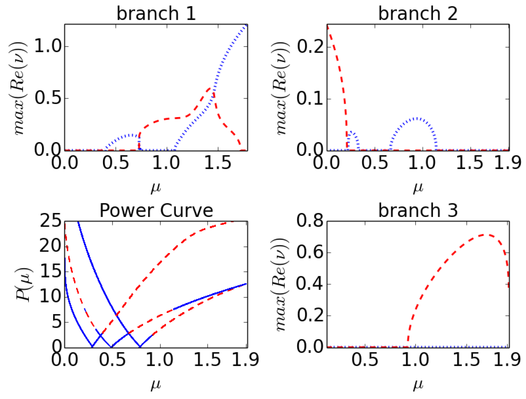
Thus, in order to find solutions of (3) for $\sigma =\pm 1$, we perform a Newton continuation in the parameter μ where the initial guess for ψ is given by the first two terms of (4). The bottom left panel of Figure 3 shows how the (optical) power $P\left(\mu \right)={\int \int \left|\psi \right|}^{2}dxdy$ of the solution grows as a function of increasing μ for $\sigma =1$, or as a function of decreasing μ for $\sigma =-1$ (from the linear limit). The first branch begins at the first real eigenvalue of U at ${\mu }_0\approx 0.286$, the second branch at ${\mu }_0\approx 0.487$, and the third branch begins at ${\mu }_0\approx 0.785$. Plots of the solutions and their corresponding time evolution and stability properties are shown in the next section.

As a general starting point comment for the properties of the branches, we point out that all the branches populate both the gain and the loss side. In the branch starting from ${\mu }_0\approx 0.286$, all four “wells” of the potential of Figure 1 appear to be populated, with the lower intensity “nodes” being more populated and the higher intensity ones less populated. The second branch starting at ${\mu }_0\approx 0.487$, as highlighted also in [19], possesses an anti-symmetric structure in x (hence the apparent vanishing of the density at the $x=0$ line). Both in the second and in the third branch, the higher intensity nodes of the potential appear to bear a higher intensity.

4. Stability of the Nonlinear Modes: Spectral Analysis

The natural next step is to identify the stability of the solutions. This is monitored by using the linearization ansatz:

$$\mathsf{\Psi }=e^{i\mu z}\left(\psi +\delta \left[a(x,y)e^{\nu z}+b^{*}(x,y)e^{{\nu }^{*}z}\right]\right)$$

(7)

which yields the order δ linear system

$$\left[\begin{array}{cc}{M}_1& M_2\\ -M_2^{*}& -M_1^{*}\end{array}\right]\left[\begin{array}{c}a\\ b\end{array}\right]=-i\nu \left[\begin{array}{c}a\\ b\end{array}\right]$$

(8)

where $M_1={\nabla }^2+U-\mu +2\sigma {\left|\psi \right|}^2$, $M_2=\sigma {\psi }^2$. Thus, $\max \left(\mathrm{Re}\right(\nu \left)\right)>0$ corresponds to instability and $\max \left(\mathrm{Re}\right(\nu \left)\right)=0$ corresponds to (neutral) stability.

In the bottom left panel of Figure 3, the power curve is drawn with stability and instability as determined by ν noted by the solid or dashed curve, respectively. The other three plots in Figure 3 show the maximum real part of eigenvalues ν for each of the three branches: the red dashed curve is the max real part of real eigenvalue pairs, and the blue dotted curve is the max real part of eigenvalue quartets with a nonzero imaginary part. The former corresponds to exponential instabilities associated with pure growth, while the latter indicate so-called oscillatory instabilities, where growth is present concurrently with oscillations. 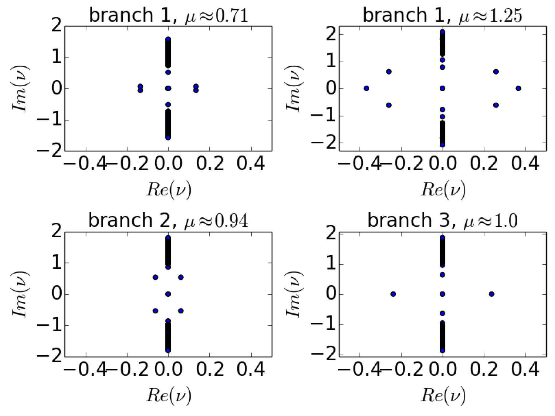In Figure 4, we plot some example eigenvalues in the complex plane for some sample unstable solutions. The dominant unstable eigenvalues within these can be seen to be consonant with the growth rates reported for the respective branches (and for these parameter values) in Figure 3.

The overarching conclusions from this stability analysis are as follows. The lowest μ branch, being the ground state in the defocusing case, is always stable in the presence of the self-defocusing nonlinearity. For the parameters considered, generic stability is also prescribed for the third branch under self-defocusing nonlinearity. The middle branch has a narrow interval of stability and then becomes unstable, initially (as shown in the top right of Figure 3) via an oscillatory instability and then through an exponential one. In the focusing case (that was also focused on in [19] for the second and third branch), all three branches appear to be stable immediately upon their bifurcation from the linear limit, yet all three of them subsequently become unstable. Branch 1 (that was not analyzed previously) features a combination of oscillatory and exponential instabilities. Branch 2 features an oscillatory instability which, however, only arises for a finite interval of frequencies μ, and the branch restabilizes. On the other hand, for branch 3, when it becomes unstable, it is through a real pair. Branches 2 and 3 terminate in a saddle-center bifurcation near $\mu =1.9$. The eigenvalue panels of Figure 4 confirm that the top panels of branch 1 may possess one or two concurrent types of instability (in the focusing case), branch 2 (bottom left) can only be oscillatorily unstable in the focusing case (yet as is shown in Figure 3, it can feature either type of instability in the defocusing case), while for branch 3, when it is unstable in the focusing case, it is via a real eigenvalue pair.

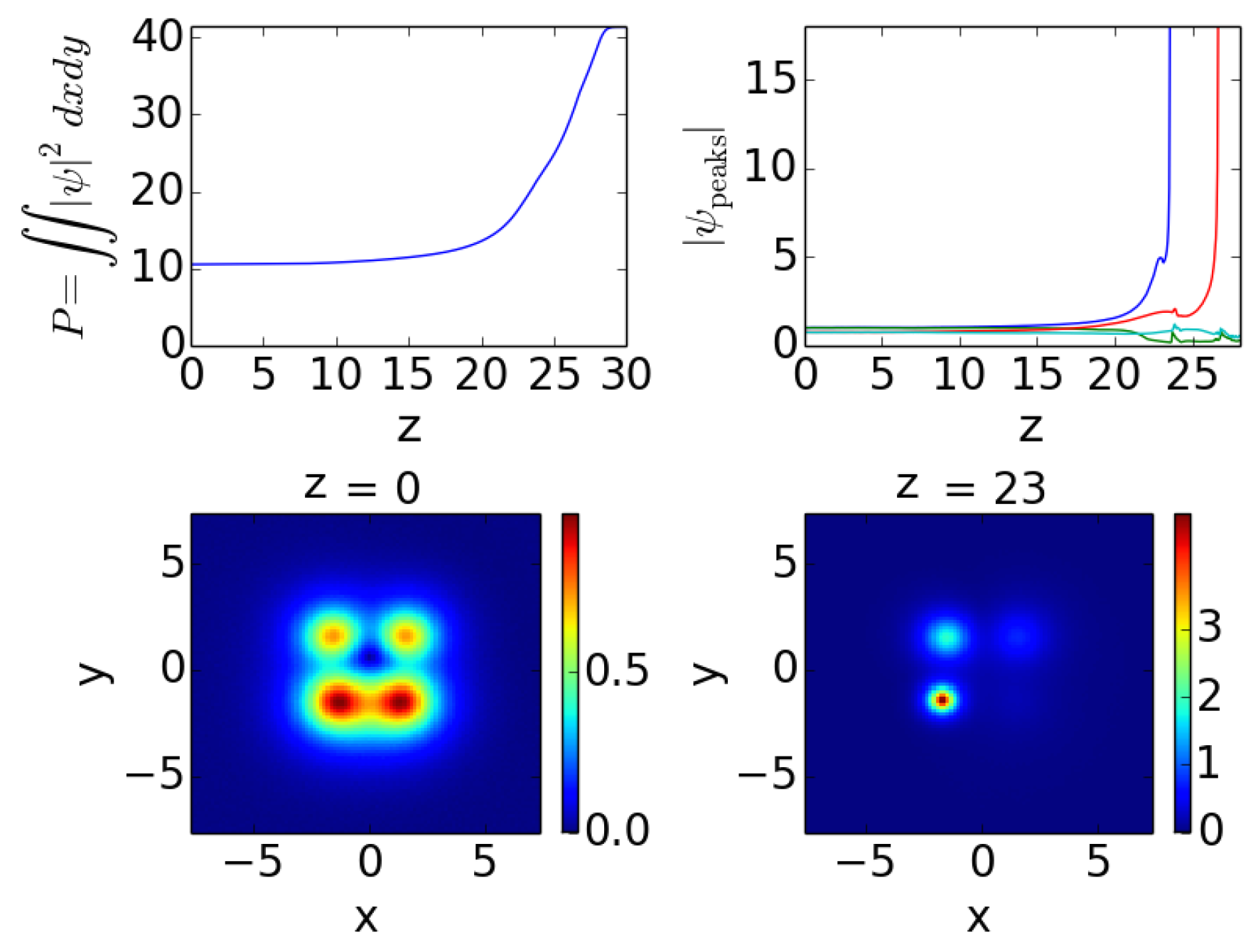
5. Dynamics of Unstable Solutions

Figure 5, Figure 6 and Figure 7 show the time evolution of three unstable solutions, one on each branch, in the focusing case for the value of $\sigma =1$. That is, they each correspond to a μ-value that is bigger than the initial discrete value ${\mu }_0$ and pertain to the focusing case. The time evolution figures show a similar feature for the unstable solutions, namely that over time the magnitude of the solutions will increase on the left side of the spatial grid. This agrees with what is expected from $\mathcal{PT}$-symmetry since the left side of the spatial grid corresponds to the gain side of the potential U. Importantly, also, the nature of the instabilities varies from case to case, and is consonant with our stability expectations based on the results of the previous section.

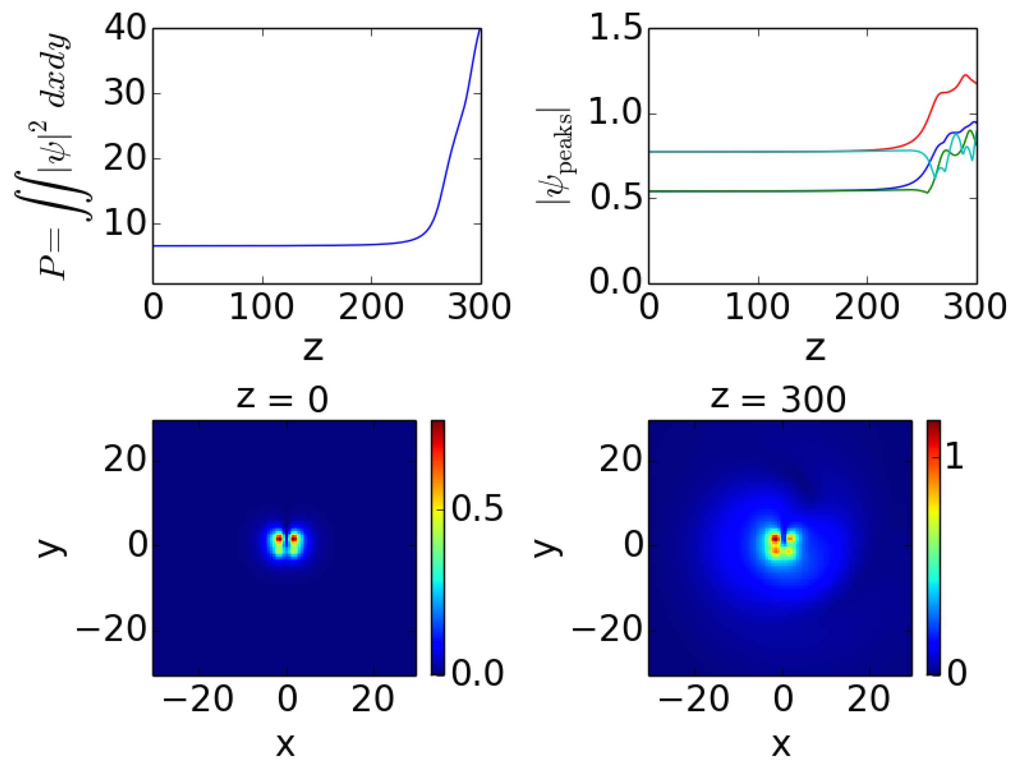
In Figure 5, branch 1 (for the relevant value of the parameter μ) features an oscillatory instability (but with a small imaginary part). In line with this, we observe a growth that is principally exponential (cf. also the top panel for the power of the solution), yet features also some oscillation in the amplitude of the individual peaks. It should be noted here that although two peaks result in growth and two in decay (as expected by the nature of W in this case), one of them clearly dominates between the relevant amplitudes.

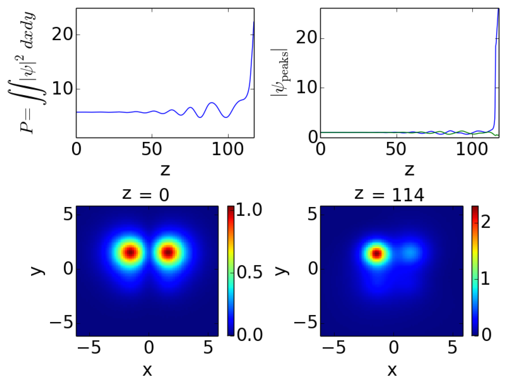
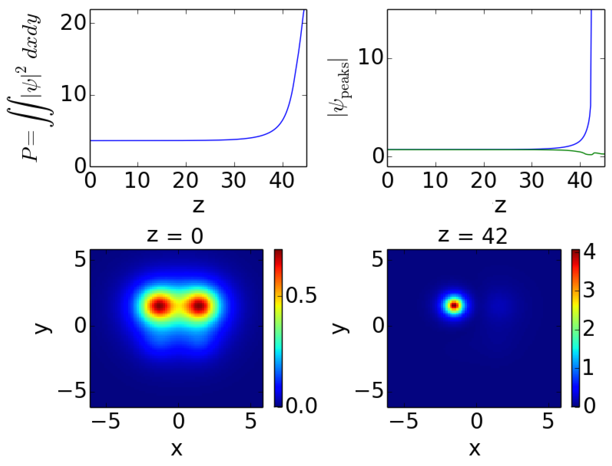
In Figure 6, it can be seen that branch 2, when unstable in the focusing case, is subject to an oscillatory instability (with a fairly significant imaginary part). Hence the growth is not pure, but is accompanied by oscillations as is clearly visible in the top left panel. In this case, among the two principal peaks of the solution of branch 2, only the left one (associated with the gain side) is populated after the evolution shown.

Lastly, in branch 3, the evolution (up to $z=42$) manifests the existence of an exponential instability. The latter leads, once again, to the indefinite growth of the gain part of the solution, resulting in one of the associated peaks growing while the other (for $x>0$ on the lossy side) features decay.

It is worthwhile to mention that in the case of branch 2—the only branch that was found (via our eigenvalue calculations) to be unstable in the self-defocusing case—we also attempted to perform dynamical simulations for $\sigma =-1$. Nevertheless, in all the cases considered, it was found that, fueled by the defocusing nature of the nonlinearity, a rapid spreading of the solution would take place (as z increased), resulting in the interference of the wave pattern with the domain boundaries. In Figure 8, we show an example where the maximum real part of the eigenvalues is $\approx 0.016$. This weak instability is of exponential type with eigenvalues having a nonzero real part lying on the real axis similar to the eigenvalues in the bottom right panel of Figure 4 (but very close to the origin). Figure 8 shows that the solution initially seems to follow the expected pattern of dominating on the gain side (left) and there is a power growth similar to the focusing cases, but accompanied by a quick increase of the spatial extent of the solution leading to interference with the computational domain boundary.

6. Conclusions and Future Challenges

In the present work, we have revisited the partially $\mathcal{PT}$-symmetric setting originally proposed in [19] and have attempted to provide a systematic analysis of the existence, stability and evolutionary dynamics of the nonlinear modes that arise in the presence of such a potential for both self-focusing and self-defocusing nonlinearities. It was found that all three linear modes generate nonlinear counterparts. Generally, the defocusing case was found to be more robustly stable than the focusing one. In the former, two of the branches were stable for all the values of the frequency considered, while in the focusing case, all three branches developed instabilities sufficiently far from the linear limit (although all of them were spectrally stable close to it). The instabilities could be of different types, both oscillatory (as for branch 2) and exponential (as for branch 3) or even of mixed type (as for branch 1). The resulting oscillatorily or exponentially unstable dynamics, respectively, led to the gain overwhelming the dynamics and leading to indefinite growth in the one or two of the gain peaks of our four-peak potential.

Naturally, there are numerous directions that merit additional investigation. For instance, and although this would be of less direct relevance in optics, partial $\mathcal{PT}$ symmetry could be extended to three dimensions. There, it would be relevant to appreciate the differences between potentials that are partially $\mathcal{PT}$ symmetric in one direction vs. those partially $\mathcal{PT}$ symmetric in two directions. Another relevant case to explore in the context of the present mode is that where a $\mathcal{PT}$ phase transition has already occurred through the collision of the second and third linear eigenmode considered herein. Exploring the nonlinear modes and the associated stability in that case would be an interesting task in its own right. Such studies are presently under consideration and will be reported in future publications.