1. Introduction
Diffusive surfaces are widely used in performance spaces since they are considered an important design aspect that improves the room’s acoustic quality and the listener’s enjoyment [
1]. Based on this, it has become important to consider their effects on the overall acoustic quality during the early architectural planning stages of a concert hall, usually investigated through geometrical acoustics (GA)-based software. Thus, a lot of effort has been put into the implementation of algorithms that take into account the scattering phenomenon due to diffusive surfaces [
2]. However, there is not a clear conclusion as to how the presence, position, and shape of these surfaces influence the acoustic parameters and the subjective perception [
3]. Consequently, the correct modeling of these surfaces in GA software is not a trivial task [
4]. Therefore, this study aims to investigate the effects of two different modeling alternatives of diffusive surfaces on the reliability and accuracy of the prediction of objective room acoustic parameters and on the perceptual aspects of a concert hall sound field. Furthermore, the surface–distance-dependent sensitivity of the listener has been investigated by comparing the reflective and diffusive configuration of one of the lateral walls. This paper is presented as a follow-up study of the previous paper [
5], which dealt with in-field measurements only.
GA-based models have been used as an alternative to both scale-model and in-field measurements after continuous improvements to their accuracy since their first development by Schroeder and Kuttruff [
6]. In particular, additional physical acoustic phenomena have been included such as diffraction and scattering [
7,
8,
9,
10,
11,
12]. Further interest in auralization has required improvements in the diffusion modeling algorithms, in binaural processing, and in reproduction techniques [
2,
13,
14]. In the last decades, several studies have investigated these aspects based on objective results and on human auditory perception [
15,
16]. The very demanding field of Virtual Reality has pointed out the need for less computational effort and more realistic auralizations [
17,
18]. Thus, it becomes important to identify the properties of room acoustics simulation that are perceptually relevant. This affects an important aspect, the modeling level of detail, which in turn might be very time-consuming. The perceptual effects of different surface modeling have not yet been fully investigated. Moreover, the task becomes harder considering that the major drawback, at the actual state of the art of the modeling software, is that the different simulation tools require different input data [
19,
20]. Thus, the material properties of surfaces or objects, such as absorption and scattering coefficients, have been shown to be aspects that significantly contribute to the uncertainty in simulations and affect their benchmarking [
21].
The level of modeling detail is considered a systematic uncertainty factor in GA models and must be decided taking into account the validity of the computational method, which depends on the dimensions of the object or surface irregularities compared to the wavelengths. Practically, this means that objects or surface irregularities that are not large compared to the wavelengths should be considered as flat surfaces with specific properties. No exact guidelines are given regarding this issue, which might lead to significant errors since a GA model might not give accurate results when using either a very detailed model or a very simple one. Several studies have investigated the most appropriate degree of detail in prediction models. Nagy et al. [
22] investigated the modeling detail of the audience area in two different kinds of software (Odeon and CATT-Acoustic), while Pelzer, Vorländer, and Maempel [
23] assessed the quality of the simulations as function of the model level of detail (LOD). Their preliminary study defined the threshold for the noticeable simplification of the structure size, 70 cm, i.e., there is no need for modeling details beyond this size. Siltanen, Lokki, and Savioja [
24] proposed an automatic geometry reduction method, which could simplify the model by reducing irrelevant small details. They concluded that, although this method could be applied in some cases, it needs to be more robust to obtain more reliable results.
The LOD in a GA model affects the generated sound field, which is strongly related to the presence and typology of diffusive surfaces; thus, their acoustical characterization becomes crucial [
25,
26,
27]. However, general rules are still used to assign the diffusive properties in simulated environments [
20,
28,
29]. As reported in Wang and Rathsam [
30], very different scattering coefficient values could produce very different sound fields. They found that models with lower LOD do appear to have greater sensitivity to the scattering coefficient selection, but the changes that have been observed in the parameters did not occur in a consistent manner across all of the halls studied [
31]. Wang and Rathsam [
30] showed that the scattering coefficient variations do not affect the results of clarity (
C80) and lateral fraction (
LF80). The most affected parameters are early decay time (
EDT) and reverberation time (
T30), which exceeded more than two JND-s (Just Noticeable Differences) from the reference model. Lam [
20] showed through simulations with different scattering algorithms that the most affected parameter from the scattering coefficient changes was
T30. Robinson, Xiang, and Braasch [
32] found that the diffusive surfaces applied on the areas of the proscenium splay help to keep stage-to-pit ratios of interaural cross-correlation (
IACC) high, but, on the other hand, distribute the energy to many reflections over time rather than concentrating it in strong early reflections, leading to decreases in
C80. Another variable, which is shown to be influential in determining the model’s sensitivity to scattering coefficient, is the listener position [
16,
30]. A receiver closer to the wall is more sensitive to changes in scattering coefficients than a receiver far from the wall. This sensitivity is particularly related to changes in
T30. The contribution of all these variables makes it more challenging to draw a general analytical formula that could relate the scattering coefficient to the acoustic parameters [
33]. The correct evaluation of these parameters must also consider the scattering variable, since the realistic environments do not have a perfect diffuse field [
34].
Based on these studies, it is evident that the accurate physical simulation of room acoustics is a very complex task. The decision of how much precision should be required from the prediction models relies on our ability to detect differences between reality and simulations. The auditory system seems to be insensitive to many aspects, e.g., small variations in the surface scattering properties [
35]. Therefore, the prediction of room acoustical perception needs to take the insensitivity of the auditory system into account. This is linked to the JND of the acoustic objective and subjective parameters, which allows for the characterization of a space and enables numerical comparison between different environments. The simulation using numerical techniques gives clues as to how a performance hall would sound when achieved. Thus, it becomes crucial for the investigation of different alternatives and for the control of the design costs. Acousticians, performers, and architects agree on the need for well-defined objective descriptors that would allow for quantifying specific subjective impressions of the acoustics of the performance space. Especially in enclosed spaces, humans are quite sensitive to the perception of sound in all its temporal, spectral, and spatial aspects, which makes a realistic auralization in room acoustics quite challenging. These three aspects are strongly affected by the presence of diffusive surfaces [
36], thus more insight into their use is needed.
In this paper, the model of a variable-acoustics concert hall has been used to investigate, objectively and subjectively, the differences between different modeling techniques of a diffusive surface, as well as the sensitivity of the acoustic parameters to the reflective and diffusive condition of one of the lateral walls. Simulations have been performed in a small shoebox-like concert hall in order to isolate the independent effects of the diffusive surfaces on the acoustic parameters. Two different acoustic configurations of one of the long lateral walls—that is, alternatively reflective or diffusive—have been considered and compared. As reported above, these configurations have been the object of formerly performed acoustic measurements [
5]; the measurement setup has been briefly described in this paper (
Section 2) in order to aid a better understanding of the investigation. The calibration of the prediction model has been performed based on four acoustic parameters: early decay time (
EDT), reverberation time (
T30), clarity (
C80), and definition (
D50). Furthermore, the interaural cross-correlation (
IACC) has been evaluated based on simulated binaural impulse responses obtained at three different distances from the variable wall. All the acoustic parameters have been obtained and compared for both reflective and diffusive configurations. A perceptual evaluation has been performed through listening tests aimed at determining the maximum distance from the lateral diffusive wall at which the acoustic scattering effects are still audible in the two different modeling alternatives. All the objective and subjective results have been compared to the in-field measurement results.
2. Methods
2.1. Room Model Setup
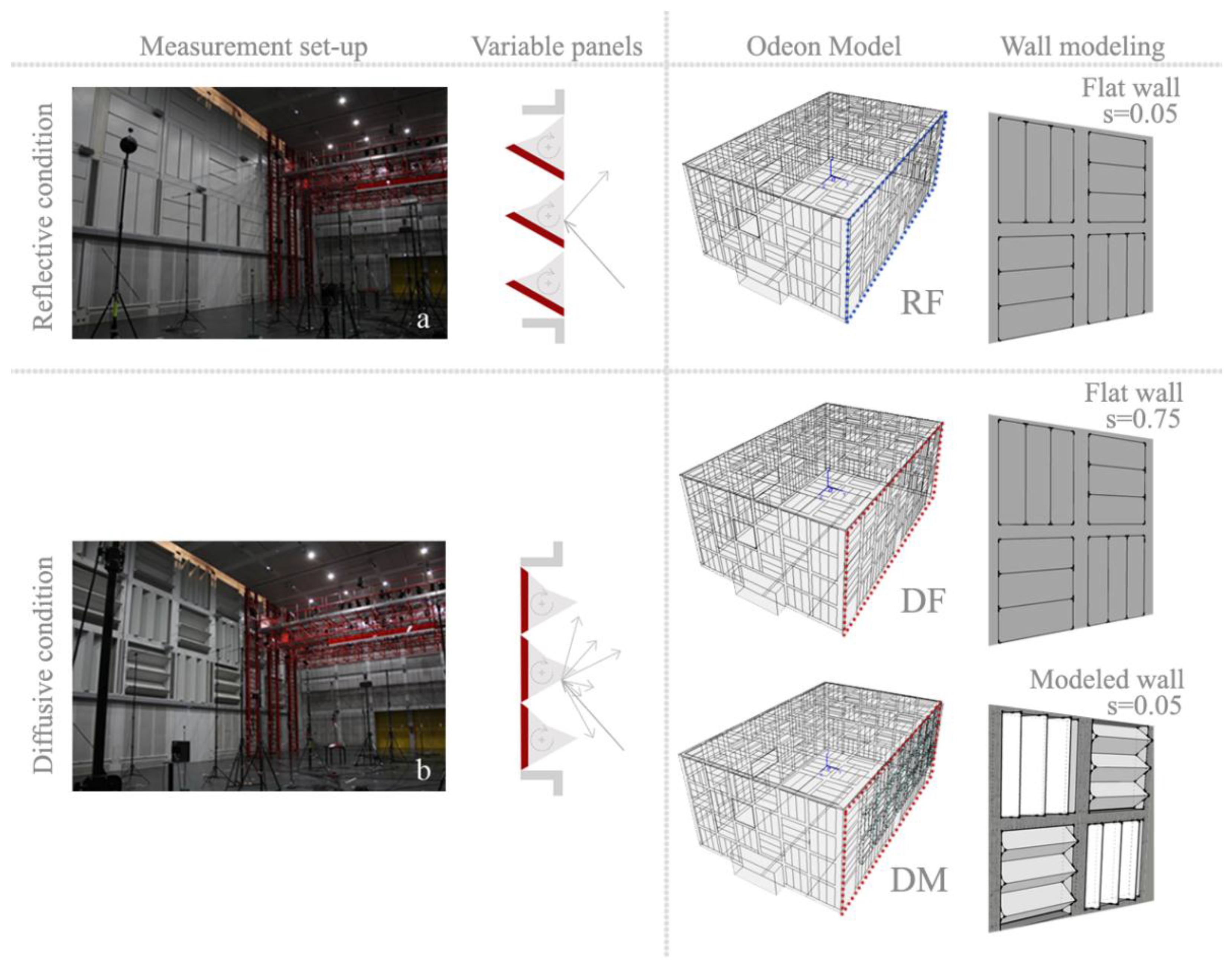
The model of a variable acoustic concert hall, the
Espace de Projection at IRCAM in Paris (
Figure 1), has been considered in this study.
Figure 2 depicts the plan of the hall, which has a rectangular geometry (24 m × 15.5 m × 10 m), and a capacity of 350 seats [
37,
38]. The geometry and the acoustical properties of the hall can be varied by controlling 172 independently rotating panels (2.3 m × 2.3 m) named
periactes. Each wall of the hall has four levels of panels. Each panel is made of three triangular prisms (
Figure 1), which have three faces with different acoustic properties: reflective, diffusive, and absorptive. The absorptive scheme of all panels has been studied in order to have two different absorption coefficients for adjacent panels. Thus, the total number of panels is divided into two parts: the absorptive side of half of the prisms is filled with a material that absorbs low frequencies (type A), while the other part of the prism has a side that absorbs high frequencies (type B). These two typologies have been obtained by using perforated metal sheets with layers of glass–wool and aluminum sheets inside. The absorptive characteristics of the materials used in the hall are given in
Table 1, namely type A and type B [
37]. The acoustic characteristics of the walls and ceiling can be modified by changing the properties of the rotating prisms. Six different acoustic conditions of the panels, that is, absorptive, reflective, diffusive, absorptive/reflective, absorptive/diffusive, and diffusive/reflective, can be obtained for the rotating prisms in the second and upper levels, while the first level of the panels can only assume two different configurations: reflective and absorptive.
The two hall configurations, whose in-field measurements results are analyzed and discussed in Shtrepi et al. [
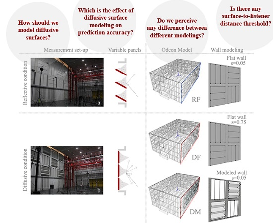
5], were chosen in this study so that one of the lateral walls was set at two different acoustic conditions: reflective and reflective/diffusive. The second condition is referred to as diffusive condition for easier understanding throughout the paper. Three CAD models have been created (
Figure 1): the reflective condition (RF), which is modeled with flat surfaces, and the diffusive condition, which has diffusive surfaces modeled in two ways, flat (DF) or explicitly modeling the 3D triangular structure (DM).
In the DF model, the prisms have been modeled as a flat surface to which a scattering coefficient equal to the scattering coefficient of the diffusive surface they represent (0.75 at 707 Hz) is assigned. This value was obtained by BEM-based simulations performed with prediction software named AFMG Reflex [
39]. Shtrepi et al. [
5] gives the results for the frequency-dependent scattering coefficient. Reflex is two-dimensional acoustics simulation software that models the reflection, diffusion, and scattering properties of a sound wave incident upon a defined geometrical structure. Some assumptions are made in these evaluations, namely that the geometry extends infinitely in the third dimension, i.e., into and out of the computer monitor screen. The surface of the sample is assumed to be perfectly rigid and does not absorb sound or allow sound to be transmitted through it. The calculation of the scattering coefficients is based on the ISO 17497-1 [
26], while the directivities are evaluated based on the Cox and D’Antonio method [
40]. In the DM model, the prisms are modeled as 3D geometries, and to each surface of the prisms a scattering coefficient equal to that of a flat surface (0.05 at 707 Hz) is assigned [
41].
The ceiling and the other walls have been fixed to be absorptive in the measurements; thus, they have been assigned absorption coefficients based on type A and type B panels’ properties (see
Table 1). The absorptive condition was also chosen for the lower level panels in all the measurements in order to avoid the strong reflections from the lower parts of the walls, as this configuration is not usual for an audience in a concert hall. Therefore, the type A and B panel properties have been assigned to these surfaces in the simulations. The floor has been considered as a hard reflective surface.
2.2. Numerical Method
Odeon 13.00 has been used as a GA software for the simulations. It is based on a hybrid calculation method, which combines an image source method (ISM) and a ray-radiosity method for early reflections (ESR) below a specified transition order (TO) with a ray-tracing/radiosity method (RTM) for late reflections [
41]. As in many other types of software, in Odeon the reflected energy can be divided into two parts, namely specular and scattered. Thus, the scattering coefficients should be provided as input data [
42]. Usually, the implementation of the scattered energy is different for different kinds of software according to the approximations made for the directional distribution of the scattered reflections [
43]. Below, two of these methods, the Hybrid Reflectance Model (HRM) and the vector Mixing (VM), are briefly described.
2.2.1. Scattering Models
The most commonly applied scattering implementations described in [
44] are the Hybrid Reflectance Model (HRM) and vector mixing (VM). The HRM is based on the decomposition of the reflected sound into specularly and diffusely deflected parts. In this method, a random number between 0 and 1 is used to determine whether the reflection is specular or scattered. This number is compared with the surface scattering coefficient(s) assigned to the surface. In case it exceeds the value of s, the scattered energy is assumed to be distributed according to Lambert’s Law, i.e., the intensity of the reflected ray is independent on the angle of incidence but proportional to the cosine of the angle of reflection [
2]. This model complies with the definition of the scattering coefficient based on ISO 17497-1, which defines it in a quantitative way as the fraction of the non-specularly reflected energy. On the contrary, the VM is based on the linear interpolation of the specular and diffuse reflection [
45], i.e., the direction of a reflection vector is calculated by adding the specular vector scaled by a factor (1-s) to a scattered vector following a certain direction that has been scaled by a factor s. This is the basic concept implemented in Odeon [
41,
46], named “vector-based scattering”, where the scattered vector follows a random direction, generated according to the Lambert distribution. Thus, the scattered reflections are also implemented from a qualitative point of view, which makes this model a more realistic approximation of the diffusive surface directivity.
2.2.2. Scattered Sound in Odeon
Odeon considers scattered sound both in the early and in the late part of the calculations. The early scattering is emitted from surface sources that are simulated each time an image source is detected. In this way, at each reflection point of the early scattering rays, a secondary source is created. This process lasts from the current reflection order up to the TO.
The late reflection method is used to treat all reflections that are not considered by the early reflection method. Every time a late ray is reflected on a surface, a small secondary source is generated, similar to a surface source. The secondary sources are assigned a frequency-dependent directionality, which may be a
Uniform, Lambert, or Oblique Lambert directivity depending on the properties of the reflection as well as the calculation settings chosen by the user.
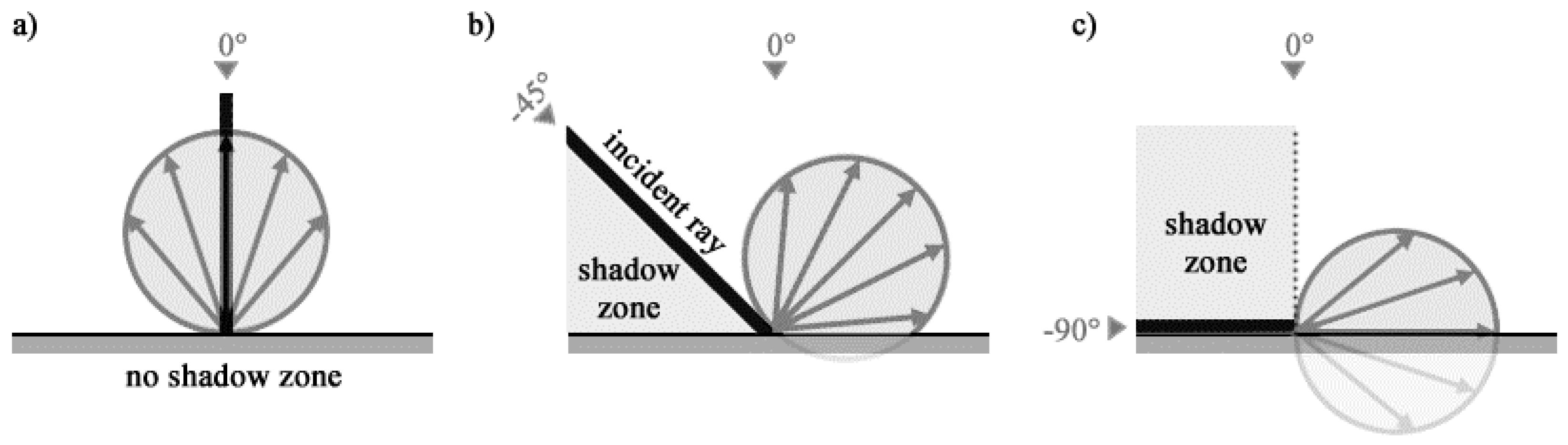
Oblique Lambert directivity is a default setting. The Uniform directivity is a simpler model that redirects the scattered reflections uniformly over a hemi-sphere above the incident point. The Lambert directivity is based on the cosine law directivity. These first two options are based on the HRM. A revised version of the Lambert directivity is the oblique Lambert (
Figure 3), which uses the concept of “vector-based scattering,” i.e., vector mixing. In this model, the orientation of the Lambert sources is obtained by taking into account the “reflection-based scattering coefficient,” which combines the scattering due to surface roughness and to surface edge diffraction. If s = 1, the reflected ray will propagate in a scattered direction conforming to the traditional Lambert’s law. If s = 0, the reflected ray will propagate in a specular direction, which is obtained from Snell’s law, i.e., the angle of incidence is equal to the angle of reflection [
2]. The “vector-based scattering” model is used when the scattering coefficient values are between 0 and 1. The resulting direction is determined using s as a weighting between the pure specular direction and the scattered direction, chosen randomly as in HRM (
Figure 4a,b). A shadow zone is created between the surface and the incident ray, where no sound reflections can be directed. Intuitively, the shadow zone is small if the scattering is high or if the incident ray is perpendicular to the surface (
Figure 3a). Conversely, it is big if scattering is low and the incident ray is oblique (
Figure 4b,c). The method is corrected to take into account the fact that for radiation angles different from 0°, the model leads to energy loss due to the fact that part of the Lambert balloon radiates energy outside the room. The correction factor varies from 1 for a radiation angle of 0° to 2 for radiation angles of 90°.
2.2.3. Reflection-Based Scattering
The scattered energy in Odeon is a combination of the surface roughness scattering coefficient s
s with the scattering coefficient due to diffraction s
d that is calculated individually for each reflection during the simulations. This combination leads to the “reflection-based scattering coefficient” s
r [
41,
46], which can be calculated from:
where s
d is the fraction of energy scattered due to diffraction and s
s is the fraction of scattering caused by surface roughness.
Surface scattering (s
s) is assumed to appear due to random surface roughness, as defined in ISO17497-1. This type of situation gives rise to scattering that increases with frequency and can be inserted by the user based on scattering coefficient measurement databases, i.e., user-based scattering. In Odeon, typical measured scattering coefficient frequency functions [
41,
46] are used to expand a mid-frequency scattering coefficient input by the user to all frequency bands. This means that only one input value for the scattering coefficients needs to be specified for a surface at a middle frequency around 707 Hz (average of 500–1000 Hz bands). These coefficients are then expanded into values for each octave band, using interpolation or extrapolation.
Surface edge diffraction (s
d) is scattering due to the surface limited size and surface edges. It is a frequency-dependent phenomenon that affects low frequencies, i.e., frequencies lower than a limiting frequency (f
g). This limiting frequency is evaluated considering the reflection path lengths, surface dimensions and distance from edge of surface, angles between surfaces, offsets, angle of incidence, etc. [
41,
46]. The s
d is handled automatically by the software since most of the factors affecting its value are not known by the user, and is considered when “reflection-based scattering” is enabled.
2.2.4. Scattering Surface Modeling (IRCAM)
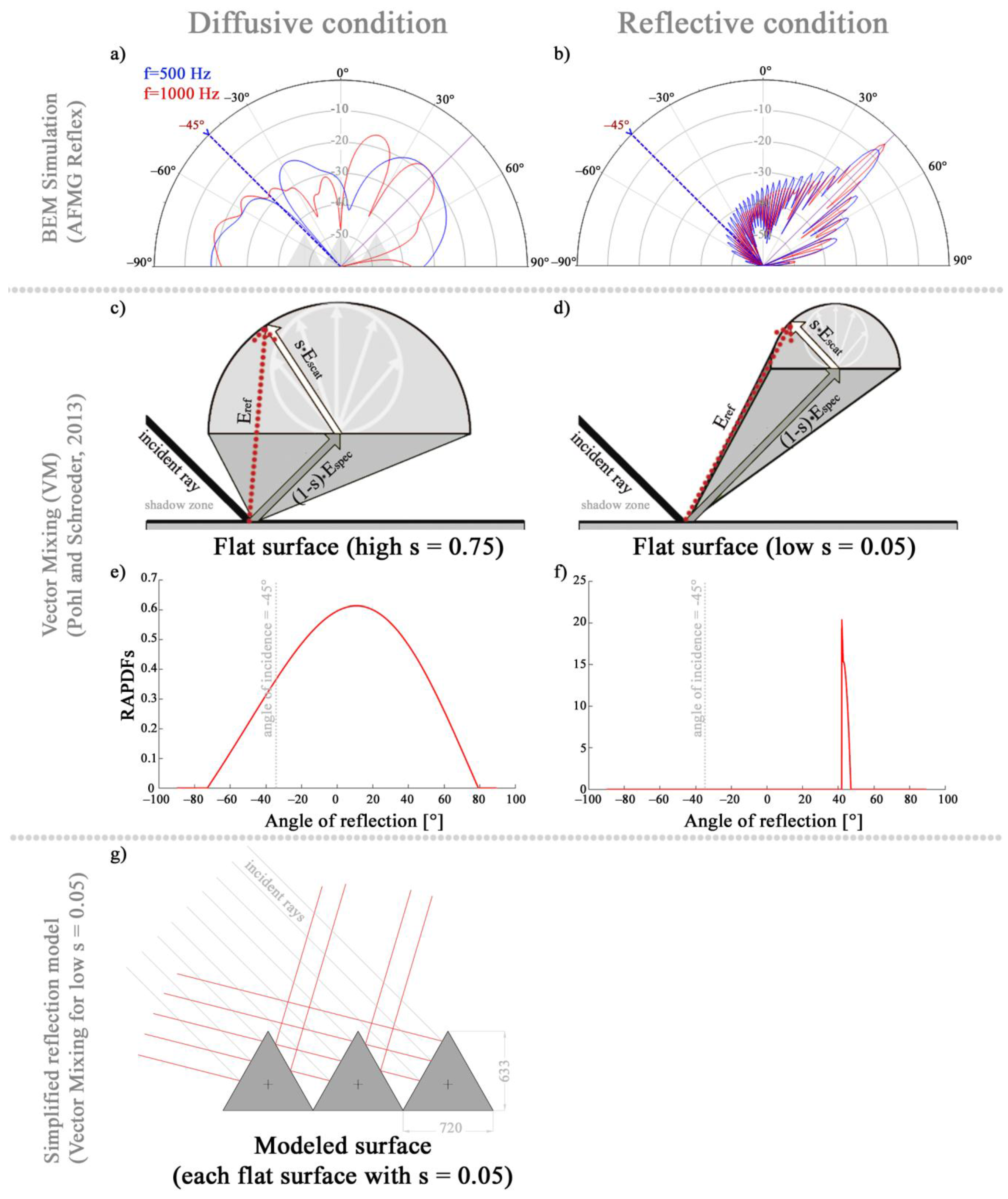
BEM-based simulations have been performed using the AFMG Reflex software in order to obtain the directivities of the triangular structure of the diffusing panels (
periactes) and compare them to the case of a hard reflective surface. The diffusion polar plots, with a resolution of 1° of the pressure amplitude of the
periactes and the flat surface, have been depicted in
Figure 4a,b for the frequencies 500 and 1000 Hz, and an incidence angle of −45°. These directivities have then been compared to the vector mixing model (
Figure 4c,d) adapted after the schemes for high and low scattering values presented in Schröder and Pohl [
44], i.e., here high s = 0.75 and low s = 0.05.
Moreover, the Reflection Angle Probability Density Functions (RAPDFs) have been calculated using the open source scripts [
47]. These functions describe the angle-wise probability for a striking energy particle/ray to get reflected under a certain angle for a given incidence angle and scattering coefficient. The models shown in
Figure 4c,d apply to the IRCAM models DF and RF (diffusive flat and reflective flat models). A simplified reflection model has been built for 3D modeled
periactes (
Figure 4g), which apply to the DM model of the room, i.e., a 3D modeled diffusive wall. In this case the incident rays have been reflected specularly, but the vector mixing model for low scattering values is applied to each reflection in Odeon. The surface edge diffraction is present in all vector mixing models, but it has not been represented in the schemes of
Figure 4.
It can be noticed that the more realistic modeling of the triangle structure (
periactes) of the walls (
Figure 4g) in the DM case (including edge diffraction) leads to more realistic directivities than modeling by vector-based scattering, i.e., vector mixing (
Figure 4c). In particular, this model does not consider that part of the energy is redirected in the direction of the incidence angle, which can be observed in the BEM simulation and in the simplified reflection model (DM).
2.3. Measurement and Simulation Setup
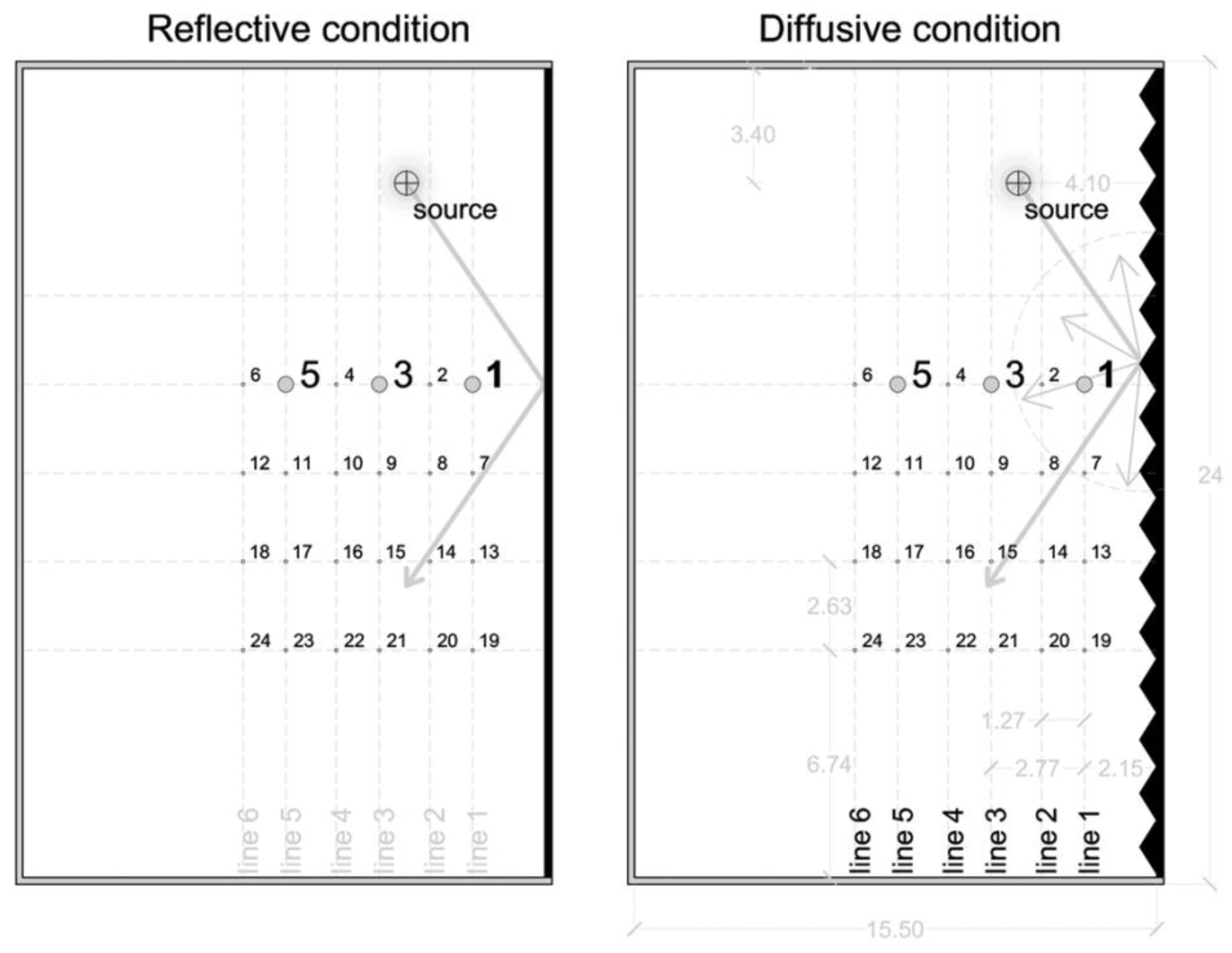
In the simulations, the 24 receivers have been located in the same positions used in the measurement setup [
5] and have been arranged in a crossed array configuration that extended to one of the two halves of the audience area (
Figure 2) at a height of around 3.70 m from the floor level. In the measurements, this height was chosen in order to reach the center of the first level of variable panels and to avoid the reflections from the absorptive panels of the lowest level. Additionally, binaural simulations have been performed in three positions (1, 3 and 5), which have been previously used for binaural measurements with an artificial head located at 3.70 m from the floor level.
The sound source was positioned midway between the axis of symmetry of the room and the lateral wall. In the measurements, it consisted of a three-way system of low-, medium-, and high-frequency sources, which were positioned at different heights, that is, at 0.40 m, 3.70 m, and 3.90 m, respectively. The position of the low-frequency source on the floor level has been considered acceptable, since humans are not able to locate the direction of such low frequencies. In the simulations, a single omnidirectional source has been used and located in the same position used in measurements for the mid-frequency omnidirectional loudspeaker.
The main input settings to perform simulations, that is, the number of rays, the maximum reflection order, and the transition order (TO), have to be decided carefully according to the aim of the simulations. First, a reasonable number of rays could be estimated by considering that an expected error of less than 1 JND is regarded as sufficient when estimating the objective acoustic parameters [
2]. However, the number of rays has been estimated following the software indication of the minimum number of rays, which is derived by taking into account the aspect ratio of the room as well as the size and number of surfaces in the geometry. This automatic number shown in the settings window was equal to 6161 rays, but a greater number was chosen to avoid artifacts and obtain higher quality in the auralizations used later in the listening tests [
18,
48]. Thus, this number was set at 100 K rays in all models and the maximum reflection order was set to 10K. A TO = 2 has been chosen based on the literature and frequently used values for similar environments [
49]. Run-to-run variations have not been considered here since, based on the literature investigations, the simulator can be considered sufficiently stable [
50,
51].
Post-processing of both measured and simulated data has been carried out using ITA-Toolbox, an open source toolbox for Matlab [
52].
Assumptions and Adjustments
In order to achieve realistic auralizations, it is important to have a well-calibrated GA model. Based on Vorländer [
53], a simulation is well calibrated when the difference between simulation and measurement is less than the JND of each objective acoustical parameter. Based upon this statement, the calibration in this study was made by comparing the simulated objective parameters to the measured ones in real conditions of the hall. Furthermore, some of the indications given in the general procedure described in Postma and Katz [
50] have been used. The calibration steps can be summarized as follows:
- (1)
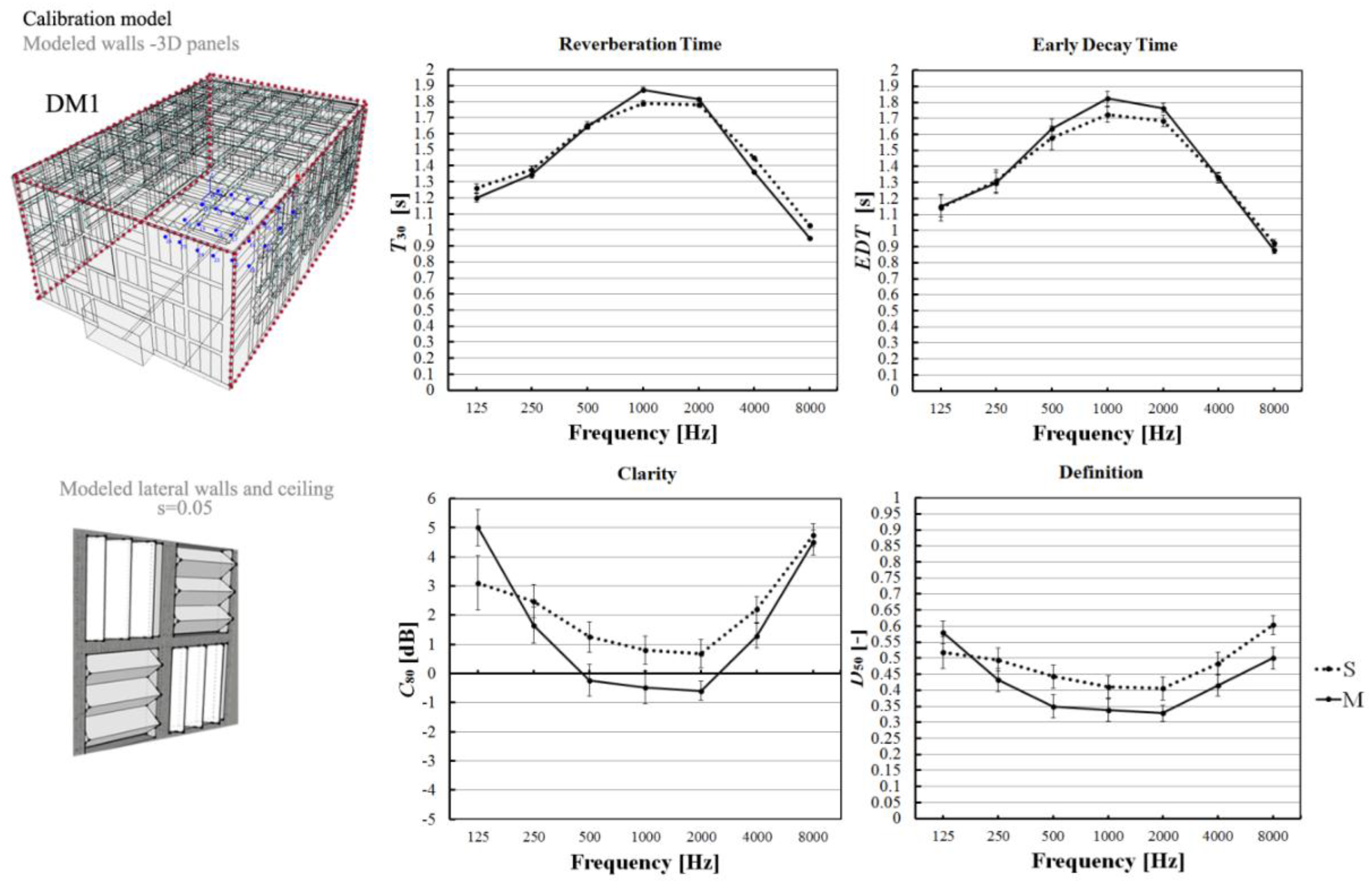
Assuming diffuse field conditions: The acoustic conditions used for this study do not represent a diffuse sound field. Since this might influence the correct estimation of the material properties, a different configuration of the hall has been used, and the diffuse field is assumed as an approximation to estimate the absorption coefficients. The model (DM1) used for the material calibration is presented in
Figure 6. This model has been chosen since it was considered to have a sufficiently diffuse field based on the achieved spatial uniformity of the reverberation time. Compared to the DM model, it assumes both long lateral walls and ceiling in diffusive condition, while the two short walls are maintained in the absorptive condition. In this configuration a more diffuse sound field is likely to be generated since larger diffusive surfaces have been used and distributed symmetrically in the room. The diffusive surfaces have been modeled as 3D prisms. This was preferred with respect to a flat surface modeling alternative, since it is a closer geometrical representation of the real room. The difference in volume between the two modeling alternatives is (V
3D − V
flat = 44.32 m
3), which could lead to differences in reverberation time of about 1%.
- (2)
Preliminary acoustical properties: As far as the absorption coefficients are concerned, in order to start the calibration process, preliminary acoustical properties (
Table 1) have been assigned to the geometrical model’s surfaces based on the data reported in the project reports and standard literature [
37,
38]. Based on the recommendations given in [
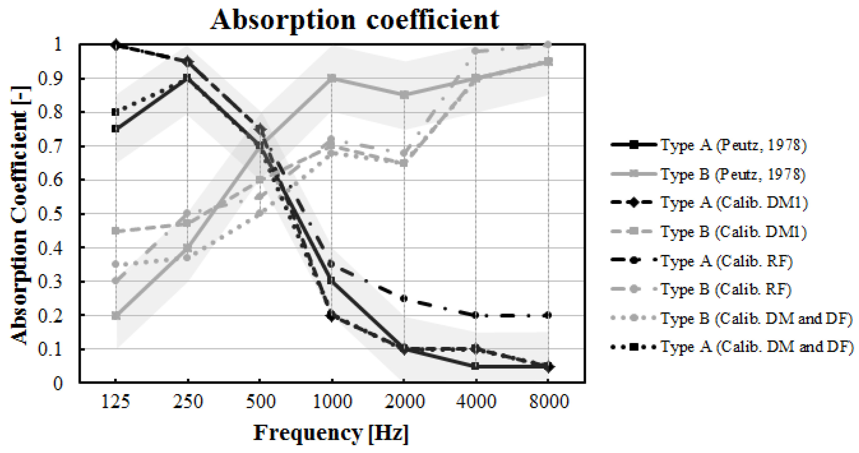
41], the scattering coefficients were set to 0.05 (707 Hz) for all flat surfaces and for the modeled 3D panels, i.e., in this case each prism surface was set 0.05 (707 Hz). Since no data could be found for the absorption coefficient of the structure and for the diffusive configuration of the panels, the same absorption coefficients have been used for these three types of surfaces based on the similar construction material (metal sheet).
- (3)
Variation of the acoustical properties: The acoustical properties of type A and B absorptive surfaces, structure, and diffusive panels have been modified since they have the most significant impact on the overall value of the equivalent sound absorption area, due to high absorption coefficients and surface extension, respectively. The variation has been performed manually and step by step until the overall mean differences (for the source and receiver configuration) between measurement and simulated results for
EDT,
T30,
C80, and
D50 resulted in less than one JND. However, the variation of the absorption coefficient of these surfaces has been restricted in order not to lose the typical acoustic properties of the material they represent (for e.g., a rockwool surface should not vary into a plastered one). Having in mind this constraint, a compromise has been made in order to stop the calibration process when differences between simulated and measured
EDT,
T30,
C80, and
D50 reached values of about one JND. The results of the material calibration are shown in
Table 1 and
Figure 5, and the results of the objective acoustic parameters after calibration are depicted in
Figure 6. It can be observed that the differences between the simulated and measured results for
C80 and
D50 are slightly above one JND. This result was still considered acceptable, based on the restriction of the absorption coefficients variations, and on the fact that the degree of tolerance for the parameters that present values of the spatial standard deviation comparable to the JND should realistically be extended beyond one JND [
50].
- (4)
Case study models: The absorptive surface properties obtained after the calibration have been assigned to the respective surfaces (type A and B) in the models of the case study (RF, DF, DM). The same properties have been used in both 3D prisms and flat surface models (DM and DF). This has been considered acceptable since the difference in volume may be considered negligible (VDM − VDF = 7.77 m3). The other surfaces such as doors, floor, and glass windows have remained the same as those used in the calibration model.
The absorptive materials of type A and type B have been slightly varied in the three models, i.e., different for the three models (RF, DF, and DM) in order to arrive at overall mean differences between measurement and simulated results for
EDT,
T30,
C80, and
D50 of less than one JND. The materials have been modified separately (
Figure 5) for the diffusive condition (DM and DF), and for the reflective condition (RF). This difference is due to the fact that the two real conditions present different materials, that is, diffusive and reflective faces of the variable panels, which could have different absorption coefficients. Since no consistent data could be found in the project documentation, it could be considered acceptable that the absorption coefficients of the type A and type B materials are affected by the uncertainty of the other unknown materials’ data.
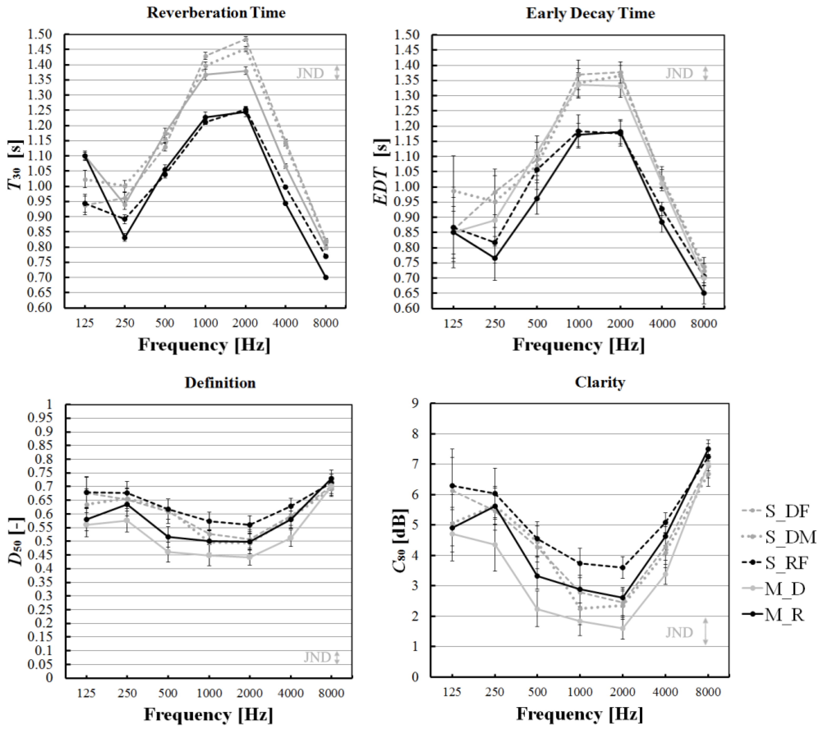
2.4. Room Acoustic Parameters
The sound fields of the reflective condition (RF) and both modeling alternatives of the diffusive conditions (DF and DM) have been investigated on the basis of ISO 3382-1 [
54]: reverberation time (
T30), early decay time (
EDT), clarity (
C80), definition (
D50), and interaural cross-correlation (
IACC). The values of the first four parameters have been presented in octave bands as mean values over all the receiver positions in order to assess the accuracy of the calibration process.
Since binaural measurements and simulations have been performed in positions 1, 3, and 5, the IACC values were evaluated and averaged over 500 Hz, 1000 Hz and 2000 Hz octave band results in each position. The IACC has been assessed by considering separately the early-arriving (0–80 ms) and late-arriving (80 ms-inf) sound since they measure different aspects of the sound field.
These parameters have been chosen since they have been used in the measurements [
5] and in the main literature concerning the study of diffusive surface effects in room acoustics. The parameters have been evaluated using the functions of ITA-Toolbox, which comply with the ISO 3382-1:2009. This was based on the study performed by Postma and Katz [
50], which suggests applying the same objective parameter estimation method for measurements and simulations in order to enable their correct comparison. By using ITA-Toolbox, it was possible to also evaluate
IACC, which is not included in the Odeon objective parameters results.
As in the calibration process, since the Just-Noticeable Differences (JNDs) report the smallest perceived difference for an objective parameter, they have been used as criteria to judge the significance of the variations induced by changes on the surface properties and surface modeling.
2.5. Subjective Investigation
The perceptual tests aimed to investigate the audible difference threshold between two acoustic reflective conditions by determining the distance threshold at which the listener no longer perceives the presence of a diffusive surface in the sound field of the room under examination. These comparisons have been made between the reflective wall condition (RF) and the diffusive wall condition modeled as flat surface (DF) and as 3D panels (DM), i.e., both RF-DF and RF-DM comparisons have been performed. Furthermore, the thresholds have been compared with the results found with measured impulse responses presented in Shtrepi et al. [
5]. Exactly the same method, named the triangular method [
55,
56], used for the comparison of the measured conditions has been deployed also for the listening test with simulated stimuli. The method implies the use of sets of three stimuli, from each of which the subject has to select the odd stimulus under forced-choice instructions. Stimulus sets (“triangles”) are constructed using A and B stimuli, such that all of the six temporal or spatial permutations (AAB, ABA, BAA, and BBA, BAB, and ABB) are used and presented in random order. The triangular method is an undirected protocol since it does not require that the nature of the difference between the A and B stimuli is provided as part of the subject’s instructions. The stimulus sets have been presented to the subjects individually through a Matlab routine and later the data have been analyzed by calculating the psychometric functions using Psignifit [
57], which is a Matlab toolbox [
58,
59]. The psychometric function is defined as the relation between a subject’s performance, i.e., here the listening test answers, and an independent variable, which is usually some physical quantity of a stimulus in a psychophysical task, i.e., here it is the difference between the reflective and diffusive condition at different distances from the variable wall. The psychometric function is given in the range [0,1] and is limited by a lower limit related to a base rate of performance in absence of stimulus (γ), i.e., the chance threshold, and to an upper limit (1−λ), where λ corresponds to the miss rate, i.e., it is the rate at which subjects lapse, responding incorrectly regardless of stimulus intensity. The shape of the function between these two limits is given by two parameters α and β, which determine two independent attributes, that is, the displacement of the function along the abscissa and its slope. These are the most important parameters since their values are crucial for the evaluation of the threshold of the psychometric function. Conversely, the upper (1−λ) and lower bound (γ) parameters are stimulus-independent, based on guessing and lapsing rates, and thus they have very little influence on the threshold estimation.
The method used for variability estimation of the parameters fitted to psychophysical data is based on Efron’s parametric bootstrap technique, which is a Monte Carlo resampling technique that relies on a large number of simulated repetitions of the original experiment. This method has been chosen since it needs a small number of data points and is applied to estimate the variability of the parameters, thresholds and slopes of the psychometric functions. The Monte Carlo simulation is based on a system that provides generating probabilities for the simulated dataset, which are the same that are hypothesized to underlie the empirical data set, i.e., the collected psychophysical data. In order to improve this system, the parametric bootstrap is used, which evaluates the maximum-likelihood fit to the real subject’s data to determine the simulated subjects underlying probability of success. The maximum-likelihood estimation is made by controlling the parameters of the psychometric function (α and β), which determine its shape based on the best fit to the experimental data.
In the experiment presented here, different triads (triangles) of the test signals have been prepared by convolving anechoic signals with the binaural impulse responses obtained in simulations at positions 1, 3, and 5 (highlighted in
Figure 1). Each triad has been built for each anechoic signal and listening position. The triads included two identical signals and one different from the other two in the comparisons RF-DF and RF-DM. These signals have been presented to the listener in a randomized order: comparison of RF with DF (RF-DF-DF, DF-RF-DF, DF-DF-RF, DF-RF-RF, RF-DF-RF, and RF-RF-DF) and comparison of RF with DM (RF-DM-DM, DM-RF-DM, DM-DM-RF, DM-RF-RF, RF-DM-RF, and RF-RF-DM). Also the receiver position and the signal type have been presented in randomized order (
Table 2). As in [
5], the test has been presented to the subjects via high quality headphones (Sennheiser HD600) without any specific headphone equalization.
As explained above, in order to build the psychometric curves, the percentage of correct answers is correlated to the stimulus intensity, which is decreased or increased by a constant step [
58,
59]. In this study, the stimulus is represented by the difference between the reflective and the diffusive condition compared at each position. Since there is no method to quantify this stimulus intensity variation between the two conditions, the stimulus intensity variation is associated with the distance from the lateral wall, which increased constantly by 2.77 m (at 2.15 m, 4.92 m, and 7.69 m for position 1, 3, and 5, respectively).
Music Samples and Test Subjects
The music stimuli presented to the listeners were created by convolving the simulated binaural impulse responses with samples of anechoic music recordings (5–6 s). Three different anechoic music samples have been chosen based on different style, tempo, and spectral characteristics [
5]:
choral recording (“Alleluia”—Randall Thompson, St. Olaf Cantorei, Anechoic Choral Recordings, Wenger),
piano solo (“Étude Op. 10 no. 4”—Frédéric Chopin, Renzo Vitale, Digital Recording)
orchestra (“Water Music Suite”—Handel/Harty, Osaka Philarmonic Orchestra, Anechoic Orchestral Music Recordings, Denon)
The subjects were chosen on a voluntary basis from professors, research assistants, and students at Politecnico di Torino (Italy). They declared their interest in acoustics and music, and all of them had experience in playing a musical instrument or singing in a choir. A total of 38 subjects participated in the listening tests. They were asked to perform an audiometric test by using an iPad-based application named uHear [
60] and wearing the same headphones (Sennheiser HD600) subsequently used in the listening test. Only 31 subjects obtained results within the “normal hearing level” and have been considered suitable to perform the perceptual listening test. This sample consisted of subjects aged between 20 and 45 years.
4. Discussion
Although this study was based on one combination of diffusive surface extension and position in the case of a simple shoebox concert hall, and only one scattering model was used and some assumptions on absorption coefficients were considered, a few useful critical comments can be made on the objective and perceptual results.
The objective results have shown that a good match can be achieved between simulated and measured results. However, the surface modeling and the calibration of the absorptive and diffusive materials require a great effort that is time-consuming. This process might lead to very different material properties compared to laboratory-measured ones. Here, the “measured absorption coefficients” have been estimated using the reverberation room method [
37,
38], but no data are available to show the degree of confirmation of these values in the application in the real room. It has been shown that laboratory measurements and in-field evaluation of absorption coefficients may differ significantly depending on the characteristics of the environment [
62]. Moreover, in our case, materials may have experienced transformations due to aging [
63]. Depending on the sound field of the environment under examination, the values of the calibrated absorption coefficients conceal the uncertainties due to initial assumptions: diffuse field, geometrical approximations, uncertainty of material characteristics based on literature, simulation algorithm, etc. As a consequence, such inaccuracies will conduct to possible wrong material choices when evaluating existing environments or newly designed ones.
The early decay time (
EDT)
showed differences between simulations and measurements smaller than one JND independently of the geometric characteristics of the model. Conversely, differences slightly higher than one JND resulted at 2000–4000 Hz for reverberation time (
T30) in the diffusive configuration (DF and DM). These were considered acceptable based on the initial constraints: restrictions on the variation of the absorption coefficients and the calibration of other two parameters, that is, clarity (
C80) and definition (
D50). Moreover, since similar differences can be noticed for simulated models DF and DM, this could not affect the results when these models are compared to the reflective model (RF). Although a great effort was put in the calibration of
C80 and
D50, differences higher than 1 JND resulted at some frequencies. Since the spatial standard deviations of these parameters, i.e., differences between different receiver positions, give results higher than or equal to the JND, the degree of tolerance should realistically be extended beyond 1 JND [
45]. In Zeng et al. [
28] the predicted
C80 was larger than the measured ones and the difference was much higher at low frequency bands when using the new method for the detailed model. This was assumed to indicate that more early sound energy is collected because of reflection and diffraction.
The objective acoustic parameters increased (
EDT and
T30) and decreased (
C80 and
D50) with increasing surface scattering as in the measurement results. This shows that in simulations also the diffusive surfaces tend to disperse reflections in space and time leading to a longer reverberation time compared to the reflective condition. In the reflective condition, a more concentrated spatial and temporal reflection is generated and successively absorbed by the absorptive surfaces that cover the ceiling and the other lateral walls. It should be highlighted that this result might change for different combinations of the diffusive and absorptive surfaces as summarized in Shtrepi at al. [
35].
The influence of the different modeling alternatives of the diffusive surfaces was more evident at positions close to the variable wall for the
IACC parameter. The values of this parameter at the positions close to the lateral wall were different for the DM and DF conditions. Robinson et al. [
64] showed that the correlation between the impulse responses at two ears at positions close to any surface is lower due to effects of the surface proximity on the impulse response of the ear oriented towards it. In this way, the binaural impulse response is affected asymmetrically on each ear channel (left and right). In the configuration investigated in this study, the right ear is oriented towards the variable wall, while the left ear is oriented towards the other lateral wall, which is absorptive. Thus, the differences in reflections between the two ears are emphasized also by this asymmetric distribution of the material properties, i.e., the correlation between the two ears decreases.
The perceptual investigation highlighted the differences between the scattered sound models shown in
Figure 4. Based on the scattering perceptual thresholds [
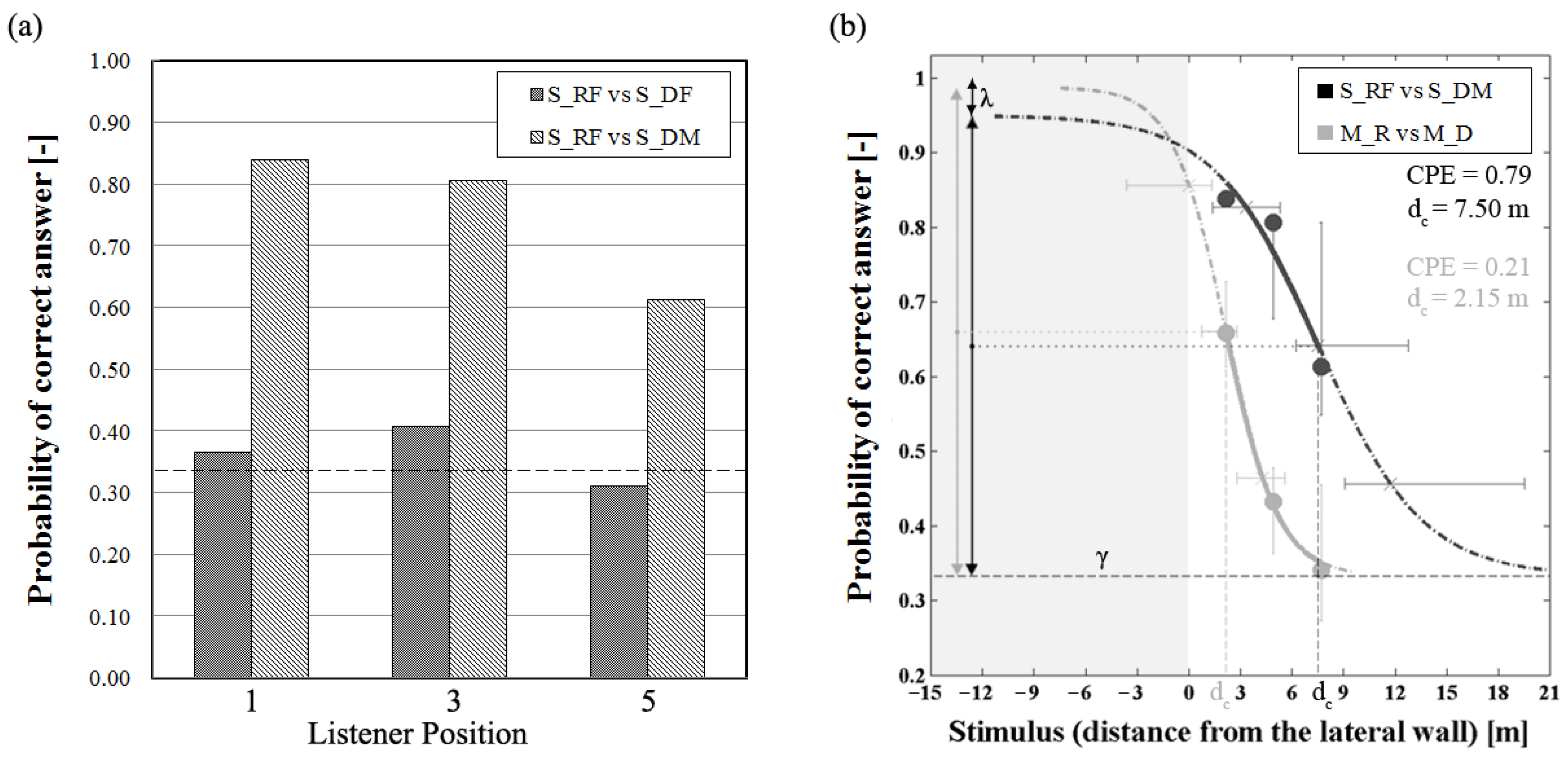
35], a difference in scattering coefficient of 0.70, which is the difference between the scattering coefficient of the diffusive surface modeled flat (0.75) and the reflective surface (0.05), should be easily perceived by the subjects. Despite this, it was not possible to find a distance threshold when the flat modeled diffusive surface (DF) was used. A distance threshold of 7.50 m was found when the DM model was used, i.e., the diffusive surfaces were modeled as 3D panels. As shown in
Figure 4g, the more realistic modeling of the diffusive walls in the DM case (including edge diffraction) leads to more realistic directivities than modeling by vector-based scattering, i.e., vector mixing, used in the DF case. In particular, when compared to the BEM simulation polar distribution, it can be noticed that the latter model does not consider the part of the energy that is deflected in the direction of the incidence angle. This might be the reason for the better audibility of diffuse reflections and better agreement with measurements.
The distance threshold is higher than the distance of 2.15 m found by performing the same listening test with measured binaural impulse responses. Such different thresholds might be due to the scattered sound model approximations. As reported in Torres, Rycker, and Kleiner [
14], some major limitations of a Lambert-based scattering model are that it neglects phase, thus neglects interference effects between specular and nonspecular scattering, whose sum constitutes the total surface scattering at a receiver position in a room. In the case of the modeled diffusive surface (DM), the scattering algorithm automatically takes into account also edge-diffraction effects, that follow a far-field type of behavior, i.e., are distance dependent [
14]. Thus, the differences between the reflective and diffusive condition are evident also at longer distances in simulations with a high degree level of detail.
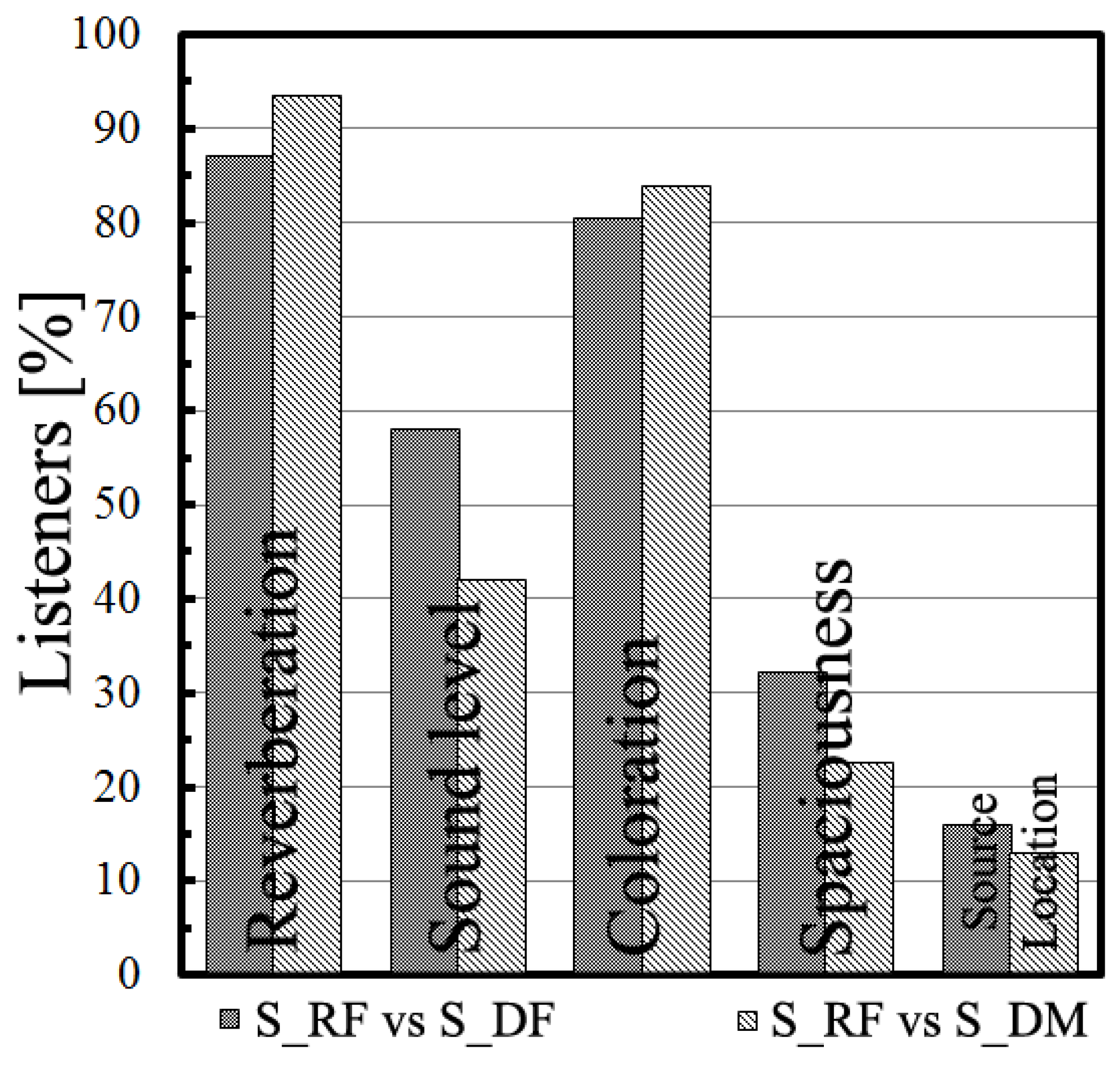
The comments at the end of each listening test highlighted that the principal effects of the perceptual evaluations within one triad of signals were coloration and reverberation. Some of the listeners claimed to perceive differences in spaciousness, sound level, and source location which might have been further emphasized by the fact that the surfaces of the hall (except for the test surface and the floor) were set in absorptive mode. The reverberation and coloration seem to be more relevant when comparing the RF to the DM model, i.e., in the conditions of 3D modeled diffusive surface. Conversely, the sound level, spaciousness and sound source location were the cues mainly used when comparing the RF to the DF model, i.e., where the diffusive surface was modeled as flat surface. The presence of reverberation might distract the listener from timbral and spatial effects of the early reflections, which were perceived at lower rate [
14]. Nevertheless, spectral and reverberation differences seem to be more consistent attributes, since the answers obtained in the RF-DM comparisons lead to correct answers way above the chance threshold.
No correlation between the subjective and the objective parameters results could be found. One possible explanation of the obtained result is that listeners contemporarily rely on different factors to make their decision. Although a multiple regression could be implemented to investigate the relationship between objective parameters and subjective responses [
65], there is a need for a single measurable parameter of more practical use.
5. Conclusions
The effects of two modeling alternatives of diffusive surfaces in geometrical acoustics (GA)-based software have been investigated, both objectively and perceptually, in a small variable-acoustics concert hall. This research aimed to isolate the independent effects that a single diffusive surface has on the simulated objective acoustic parameters and perceptual experience based on simulated impulse responses. Thus, two different conditions of the hall, where one of the lateral walls assumed reflective (RF) and diffusive characteristics (DF and DM), have been considered. The two modeling alternatives of the diffusive condition were built based on the simulations state of the art and considering the limits of a possible increase of the modeling level of detail. In the first model (DF) diffusive prisms have been modeled as a flat surface to which a scattering coefficient equal to the scattering coefficient of the diffusive surface they represent (0.75 at 707 Hz) was assigned. In the second model (DM) the diffusive prisms have been modeled as 3D panels with their geometrical characteristics, and to each surface of the prisms a scattering coefficient equal to that of a flat surface (0.05 at 707 Hz) was assigned.
The objective evaluation has been carried out by analyzing the variation of the ISO 3382-1 acoustic parameters T30, EDT, C80, D50, and IACC in each of the three models (RF, DF, and DM). The perceptual evaluation aimed at determining the maximum distance from the wall at which the listeners could no longer perceive the difference between the reflective and diffusive condition. Furthermore, it aimed to investigate if this distance is influenced by the different modeling alternatives of the diffusive surfaces in GA-based software. The psychometric functions have been evaluated and statistically analyzed using the Psignifit toolbox (version 2.5.6).
The main conclusions of this work can be summarized as follows:
A good match and similar trends can be achieved between simulated and measured results regardless the geometric modeling of the diffusive surfaces. However, this requires different material calibrations with respect to the diffusive properties.
Listeners in a simulated performance space can perceive the presence of different acoustic scattering properties, and it was found that this perception is related to the distance from the diffusive surface and to their geometric modeling.
A more realistic geometrical modeling of the diffusive surfaces leads to more realistic reflections directivities than when vector mixing model is used. This might be the reason for the better audibility of diffuse reflections and better agreement with measurements.
Distance thresholds in simulations (7.50 m) are higher than in real measurements (2.15 m) due to the scattered sound model approximations: reflections and diffraction.
No correlation between the subjective and the objective parameters results could be found, thus there is a need for further investigation on new single measurable parameter of a more practical use.
Most of the listeners were sensitive to the presence of acoustic scattering also at distant positions from the diffusive surfaces in simulations. Therefore, the use of these surfaces in large concert halls might affect the uniformity distribution of the acoustic quality in a large group of listeners and influence the design goals.
Future work could involve objective and perceptual investigations concerning the comparison of different simulation algorithms, by considering different locations and extensions of the diffusive surfaces in a broader number of hall volumes and shapes.
Many musicians in the stage area are frequently located at distances from the stage walls that are comparable or shorter than the distance threshold found here, thus they are expected to perceive the differences between different modeling alternatives and surface scattering properties assigned in simulations. Based on this, the results of this work become relevant when modeling the surfaces of the stage area and when performing listening tests concerning the acoustics quality of the stage.
Finally, the findings of this study could be useful to further improve the GA-based software guidelines for accurate simulations. Moreover, they might be used in future studies to perform investigations on surface-optimized topology within performance spaces, thus helping to control the design costs.


