A Timed Colored Petri Net Simulation-Based Self-Adaptive Collaboration Method for Production-Logistics Systems

Abstract

Complex and customized manufacturing requires a high level of collaboration between production and logistics in a flexible production system. With the widespread use of Internet of Things technology in manufacturing, a great amount of real-time and multi-source manufacturing data and logistics data is created, that can be used to perform production-logistics collaboration. To solve the aforementioned problems, this paper proposes a timed colored Petri net simulation-based self-adaptive collaboration method for Internet of Things-enabled production-logistics systems. The method combines the schedule of token sequences in the timed colored Petri net with real-time status of key production and logistics equipment. The key equipment is made ‘smart’ to actively publish or request logistics tasks. An integrated framework based on a cloud service platform is introduced to provide the basis for self-adaptive collaboration of production-logistics systems. A simulation experiment is conducted by using colored Petri nets (CPN) Tools to validate the performance and applicability of the proposed method. Computational experiments demonstrate that the proposed method outperforms the event-driven method in terms of reductions of waiting time, makespan, and electricity consumption. This proposed method is also applicable to other manufacturing systems to implement production-logistics collaboration.

1. Introduction

Nowadays, in order to survive in the competitive market, manufacturing enterprises have changed the mode of production from mass production to customized and on-demand production with small batches and short cycles. Flexible manufacturing systems (FMS) can produce a mid-volume and a mid-variety of products and allow rapid changes between them [1]. However, due to external and internal fluctuations, the machining environment changes dynamically and the optimal process plan and schedule becomes less efficient or even infeasible. In order to solve the aforementioned problems, many research efforts have been made by using the advanced technologies, such as Internet of Things (IoT) [2], cloud computing (CC) [3], cyber-physical systems (CPS) [4], and service-oriented technologies (SOT) [5]. Based on these types of research and technology, real-time and multi-source manufacturing data and logistics data are easier to access than ever before [6]. The advances in IoT and CC have provided promising opportunities to further address the aforementioned problems. Firstly, real-time and accurate information of manufacturing things can be collected by using embedded devices and sensors, such as radio frequency identification (RFID) sensors, etc. Real-time information capturing and integration architecture of the internet of manufacturing things has been presented to support optimal control and decision during manufacturing execution [7]. Secondly, researchers and practitioners have proposed a variety of cloud services, ranging from product design, manufacturing, performance analysis, and exception diagnosis. For example, an architecture of scientific workflow management system based on a cloud manufacturing service platform has been proposed to formalize and structure distributed scientific processes [8].

An FMS is a computerized and highly automated production system that integrates a set of computer numerically-controlled machines and a material handling system [9]. In an FMS, the automated guided vehicle (AGV) is widely used for transportation among production cells and warehouses. Petri nets (PNs) are widely used to model, analyze, and control FMSs [10,11] and other discrete event systems (DES) [12,13] since they can well depict the relation between equipment status and operations. The simultaneous scheduling of different components of FMS has drawn research attentions in recent years. For instance, Baruwa and Piera investigated the simultaneous scheduling of machines and AGVs using a Petri net approach [14]. Raj et al. studied the simultaneous scheduling of machines and tools in an FMS [15]. However, in real production, the manufacturing environment changes dynamically because of uncertainties and disturbances, which makes the schedule less efficient or infeasible [16]. Moreover, the scheduling tasks are complicated and time-consuming. With respect to the topic of production and logistics in manufacturing systems, a lot of research work has been done, such as simultaneous scheduling of production and logistics [17]. Only a few researchers have focused on works dealing with IoT-based production-logistics collaboration [18,19]. Despite significant achievements, several challenges still exist in the production-logistics collaboration. These challenges are summarized as follows:

(1)

How can the advantages of IoT and CC technology be leveraged to model the behaviors of key production and logistics equipment and make the equipment ‘smart’? Generally, key equipment such as machines and AGVs simply execute the commands of the preset programs or workers. The equipment is not aware and cannot make decisions based on dynamic changes in the manufacturing environment. Thus, they cannot adjust the schedule according to real-time scenarios.

(2)

How can a production-logistics collaboration strategy be designed to undertake active response and self-organizing configuration? In traditional manufacturing systems, the behaviors of both machines and AGVs are event-driven. The logistics task generates after the machine processing is finished. However, this kind of production-logistics system is time-consuming, which may cause high costs.

(3)

How can key manufacturing resources be integrated with cloud service platforms to provide the foundations for production-logistics collaboration? Despite the achievements in Industry 4.0 and CPS models, it is not clear how to implement production-logistics collaboration in an FMS. An integrated framework is needed to describe the relationships among different components of the FMS and the cloud service platform.

In order to address these challenges, this paper investigates the mechanism of production-logistics collaboration in an FMS. A self-adaptive collaboration method based on a timed colored Petri net (TCPN) is proposed for production-logistics systems. The proposed method combines the schedule of token sequences in the TCPN model with real-time status of key production and logistics equipment such as machines and AGVs. In the simulation experiment, colored Petri nets (CPN) Tools is used to validate the performance and applicability of the proposed method. Three key performance indicators (KPI), including waiting time, makespan, and electricity consumption are considered. Several contributions are significant to the literature. In the first place, intelligent modeling of key equipment is implemented by equipping the equipment with embedded devices or sensors and establishing a knowledge base. The behaviors of key equipment are associated with the TCPN model. Thus, key production and logistics equipment, such as machines and AGVs, are made ‘smart’ to actively publish logistic tasks and actively request logistics tasks. Secondly, an integrated framework based on a cloud service platform is introduced to provide the basis for self-adaptive collaboration of production-logistics systems. The capacity and real-time status of key equipment are packaged as cloud services to be published on the cloud services platform. Thus, the production-logistics collaboration is switched to the matching of tasks with services. Thirdly, simulation studies are carried out to compare the proposed method with the event-driven method. The results present the outperformance of the proposed method in reductions of waiting time, makespan, and electricity consumption.

The rest of this paper is organized as follows. Section 2 introduces an integrated framework based on cloud service platform for production-logistics systems. Section 3 performs a detailed description of a TCPN-based self-adaptive collaboration method for IoT-enabled production-logistics systems. Section 4 presents an industrial case and a simulation experiment to evaluate the fulfillment and feasibility of the proposed method. Section 5 draws conclusions and describes future work activities.

2. Framework

In order to solve the aforementioned problems, an integrated framework based on a cloud service platform for production-logistics systems is introduced as shown in Figure 1. The proposed framework is composed of three layers, namely the physical layer, the cyber layer, and the application layer. The aim of this framework is to provide the foundations for production-logistics collaboration.

2.1. The Physical Layer

The physical layer consists of manufacturing resources, such as smart production cells, smart AGVs, materials, pallets, RFID readers and tags, etc. These manufacturing objects are equipped with embedded devices and sensors so that they can perceive real-time status of themselves as well as others. The objective of the physical layer is to realize real-time status information perception and interaction between machine tools, AGVs, buffers, workers, and cloud clients.

In a smart production cell, cameras and sensors are used to perceive real-time status of machines during machine processing. RFID tags are attached to machines, materials, pallets, and workers. Thus, RFID readers can obtain the location information and basic information of these manufacturing objects. For a smart AGV, embedded devices and sensors are used to collect real-time status information. For example, global positioning system (GPS) devices can capture real-time location information in a real manufacturing environment. An AGV with RFID tags can be associated with the pallet and materials that are being transported. Hence, by integrating manufacturing objects with IoT technology, real-time status information is more easily collected and accessed. The real-time status information can be divided into five parts, including product information, production cell information, AGV information, storage information, and manpower information.

2.2. The Cyber Layer

The cyber layer is composed of cloud computing centers and other computational resources, such as servers, processors, disks, and databases, etc. These computational resources provide the capabilities that include data storage, data processing, statistical analysis, and simulation. This layer aims at managing the collected information and providing the basis for decision-making.

In this layer, there are two steps to implement the intelligent modeling of key equipment. Firstly, data cubes are constructed to store the collected status information. A large number of data cubes compose a data warehouse. On-line analytical processing (OLAP) tools are used to process the data in the data warehouse. Secondly, virtual devices including virtual machines and virtual AGVs are designed based on the collected status information to monitor and control the behaviors of key equipment. The characteristic of a virtual machine contains the location, current operation, temperature, and vibration, etc. The characteristic of a virtual AGV contains the location, current operation, speed, and voltage, etc. Thus, real-time status of key equipment can be associated with the characteristic of virtual devices.

2.3. The Application Layer

In the application layer, a cloud services platform is constructed to provide cloud services and publish logistics tasks through cloud clients. The cloud client includes thin clients, mobile apps, and web browsers, etc. Thus, these cloud services can be well integrated with embedded devices and mobile devices, such as smartphones and tablets. In this layer, a TCPN model is developed to depict and control the behaviors of key equipment by adjusting the schedule of token sequences. A rule base and a knowledge base are set up based on real-time data and historical data. The rules and knowledge are learned from historical data and are tuned by real-time data.

In order to implement production-logistics collaboration, a self-adaptive collaborative strategy is designed as follows. Firstly, smart machines actively publish logistics tasks on the cloud services platform at the beginning of machine processing. Then, smart AGVs actively request the logistics tasks once published and provide logistics services. The nearest AGV with enough space will be selected as a feasible option. The selected AGV will accept or reject the logistics task according to the priority of the task. Real-time routing optimization is implemented during the empty trip and the transport.

For the data communication between key equipment and servers, a variety of connection technologies and protocols for wireless communication including fourth-generation (4G) connectivity and Wi-Fi access can be used to realize the proposed framework. 4G Long-Term Evolution (LTE) standard provides data transfer rates of 100 Mb/s in the downlink and 50 Mb/s in the uplink, which is enough to satisfy the demand of speed and time [20,21]. Thus, the proposed framework is technically feasible.

3. Method

In this section, a self-adaptive collaboration method is proposed for IoT-enabled production-logistics systems. TCPN is used to develop the model of production-logistics systems. The mechanism of self-adaptive collaboration between production and logistics is investigated. Conflict-free routing is not dealt with in the proposed TCPN model.

3.1. Problem Definition and Notations

In this part, the production-logistics problem and corresponding notations are given as follows. Generally, an FMS consists of a set of computer numerically controlled machines and a material-handling system. AGVs are widely used to facilitate the transport of raw materials, work in process (WIP), finished products, and waste materials between warehouses and production cells. Consider an FMS that contains a set of machines and a set of AGVs. A set of jobs is to be processed on a list of machines in a predetermined order. A machine can perform one operation once. The warehouse and every production cell has an input buffer and an output buffer served as the unloading point and the loading point respectively. Both the number and the loading space of AGVs are limited.

The notations used in the problem statement, algorithm description, and throughout the paper are as follows:

• $i,h$: machine
• $j$: job
• $\left(i,j\right)$: an operation that job $j$ is processed on machine $i$
• $\left(i,j\right)\to \left(h,j\right)$: job $j$ should be firstly processed on machine $i$ and then on machine $h$
• $t$: current time
• $y_{ij}$: starting time of operation $\left(i,j\right)$
• $p_{ij}$: processing time of operation $\left(i,j\right)$
• $\Delta T_{ij}^R$: remaining time of operation $\left(i,j\right)$
• $P_{ihj}$: priority of logistics task between operation $\left(i,j\right)$ and operation $\left(h,j\right)$
• $Q_{ih}$: volume of parts transported from machine $i$ to machine $h$
• $Q_k^A\left(t\right)$: remaining space of AGV $k$ at time $t$
• $L_r$: path length of road segment $r$
• $v_k$: speed of AGV $k$
• $T_{ik}^{\left(r\right)}$: time cost of AGV $k$ passing road segment $r$
• $T_{ik}$: time cost of AGV $k$ arriving at machine $i$
• $\Delta T_{ihk}^A$: time cost of AGV $k$ going from machine $i$ to machine $h$
• $\Delta T_{total}$: total waiting time
• $\Delta T_{ihj}$: waiting time between operation $\left(i,j\right)$ and operation $\left(h,j\right)$
• $\Delta T_{ij}^{WB}$: waiting time of job $j$ on machine $i$ before processing
• $\Delta T_{ij}^{WA}$: waiting time of job $j$ on machine $i$ after processing
• $C_{\max }$: makespan
• $C_j$: completion time of job $j$
• $C_{ij}$: completion time of operation $\left(i,j\right)$
• $E_{total}$: total electricity consumption
• $E_M^{\left(i\right)}$: electricity consumption of machine $i$
• $E_{AGV}^{\left(k\right)}$: electricity consumption of AGV $k$
• $P_{MP}^{\left(i\right)}$: average power of machine $i$ when processing
• $P_{MI}^{\left(i\right)}$: average power of machine $i$ when idle
• $P_{AGV}^{\left(k\right)}$: average power of AGV $k$

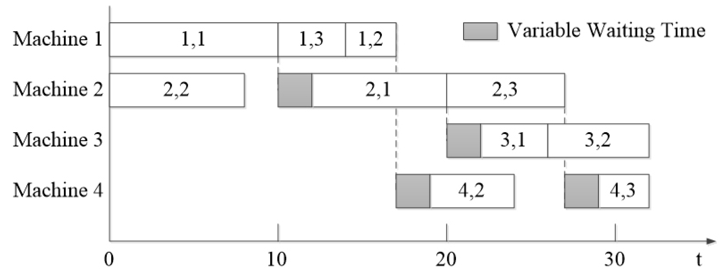
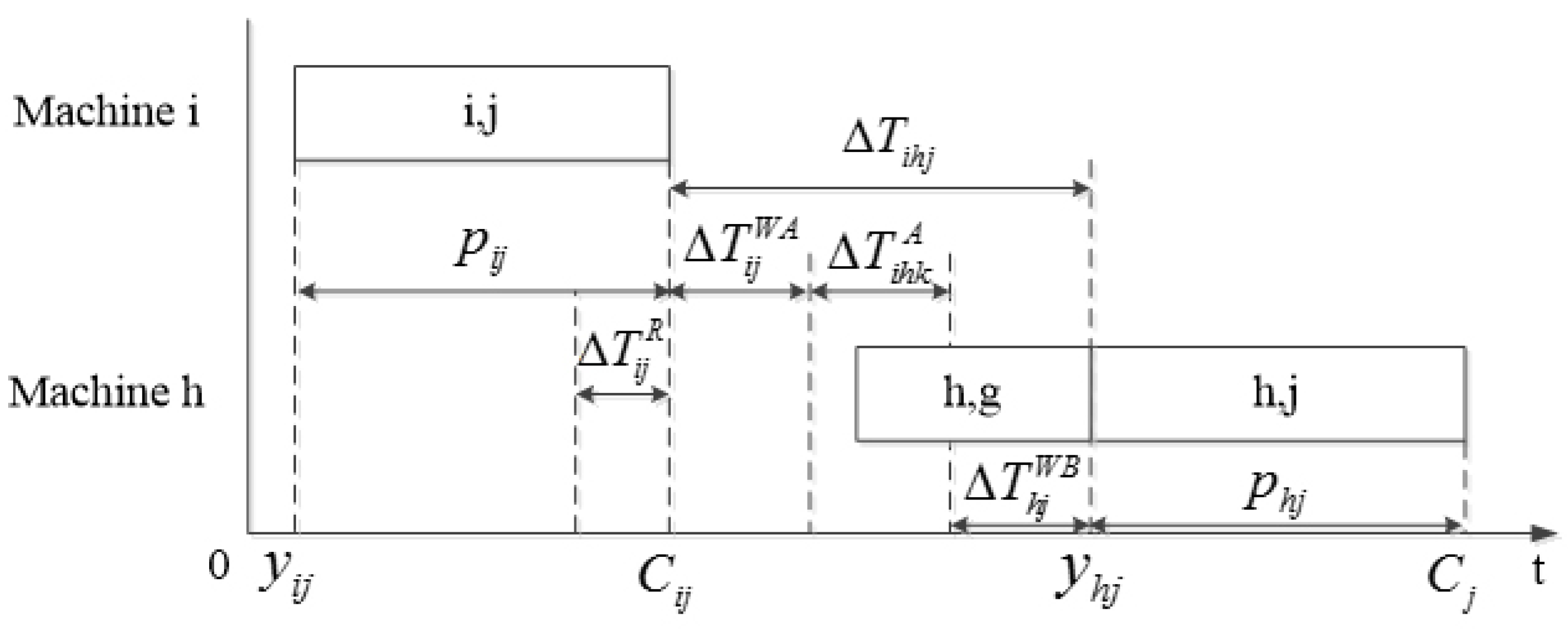
Assuming that a feasible schedule plan is given as in Figure 2, first, the job $j$ is processed on the machine $i$. The starting time of operation $\left(i,j\right)$ is $y_{ij}$. The processing time of operation $\left(i,j\right)$ is $p_{ij}$. The completion time of operation $\left(i,j\right)$ is $C_{ij}$. The remaining time of operation $\left(i,j\right)$ is $\Delta T_{ij}^R$. Then, after the operation $\left(i,j\right)$, the WIP is transported to the next machine $h$. The waiting time between operation $\left(i,j\right)$ and operation $\left(h,j\right)$ is $\Delta T_{ihj}$. The waiting time of the job $j$ on machine $i$ before processing is $\Delta T_{ij}^{WB}$. The time cost of AGV $k$ going from machine $i$ to machine $h$ is $\Delta T_{ihk}^A$. The waiting time of the job $j$ on machine $i$ after processing is $\Delta T_{ij}^{WA}$. Next, the job $j$ is processed on the machine $h$. The starting time of operation $\left(h,j\right)$ is $y_{hj}$. The processing time of operation $\left(h,j\right)$ is $p_{hj}$. The completion time of operation $\left(h,j\right)$ is $C_{hj}$. The completion time of the job $j$ is $C_j$.

3.2. Timed Colored Petri Net Model

Colored Petri nets (CPNs) form a graphical language for constructing models and analyzing properties of concurrent systems and distributed systems, which extends PNs with data types, functions, and modules.

A CPN is a directed bipartite graph that includes two types of nodes, namely the place and the transition [22]. The nodes are connected via directed arcs. The place is used to describe resources and status in the system, which contains colored tokens. The colored token is used to describe the entity attributes. The transition is used to describe the event in the system, which can be fired based on the preconditions of input arc expressions and guards. In a CPN, places, transitions, arcs, and guards are graphically represented by ellipses, rectangles, arrows, and parentheses respectively.

In order to evaluate the performance of the model system, TCPNs are introduced with a global clock to represent the model time [23]. Each token has a time attribute called the time stamp which describes the earliest time at which a token becomes available. Hence, both the temporal behavior and the logical behavior can be described by TCPNs explicitly in a concise manner.

The definition of a TCPN can be formalized as follows [24].

A TCPN is defined as a nine-tuple, $TCPN=\{P,T,A,\mathrm{\Sigma },N,C,G,E,I\}$ which satisfies the following conditions:

• $P=\left\{p_1,p_2,\mathrm{...},p_m\right\}$ is a finite set of places.
• $T=\left\{t_1,t_2,\mathrm{...},t_n\right\}$ is a finite set of transitions, $P\cup T\ne \varnothing$ and $P\cap T=\varnothing$.
• $A=\left\{a_1,a_2,\mathrm{...},a_l\right\}$ is a finite set of directed arcs, $A\subseteq P\times T\cup T\times P$.
• $\mathrm{\Sigma }$ is a finite set of non-empty color sets.
• $N$ is a node function defined from $A$ into $P\times T\cup T\times P$.
• $C$: $P\to \sum$ is a color set function that assigns a color set to each place.
• $G$: $T\to EXPR$ is a guard function that assigns a guard to each transition $t$ such that:

  $$[Type(G(t))=Bool\wedge Type(Var(G(t)))\subseteq \mathrm{\Sigma }].$$
• $E$: $A\to EXPR$ is an arc expression function that assigns an arc expression to each arc $a$ such that:

  $$\forall a\in A:\left[Type\left(E\left(a\right)\right)=C{\left(p\left(a\right)\right)}_{MS}\wedge Type\left(Var\left(E\left(a\right)\right)\right)\subseteq \mathrm{\Sigma }\right]$$

  where $p(a)$ is the place of $N(a)$.
• $I$: $P\to EXPR$ is an initialization function that assigns an initialization expression to each place $p$ such that:

  $$\forall p\in P:\left[Type\left(I\left(p\right)\right)=C{\left(p\right)}_{MS}\wedge Type\left(Var\left(I\left(p\right)\right)\right)\subseteq \varnothing \right].$$

  $Type(v)$ denotes the type of the variable $v$. $Var(expr)$ denotes a set of variables in the expression $expr$.

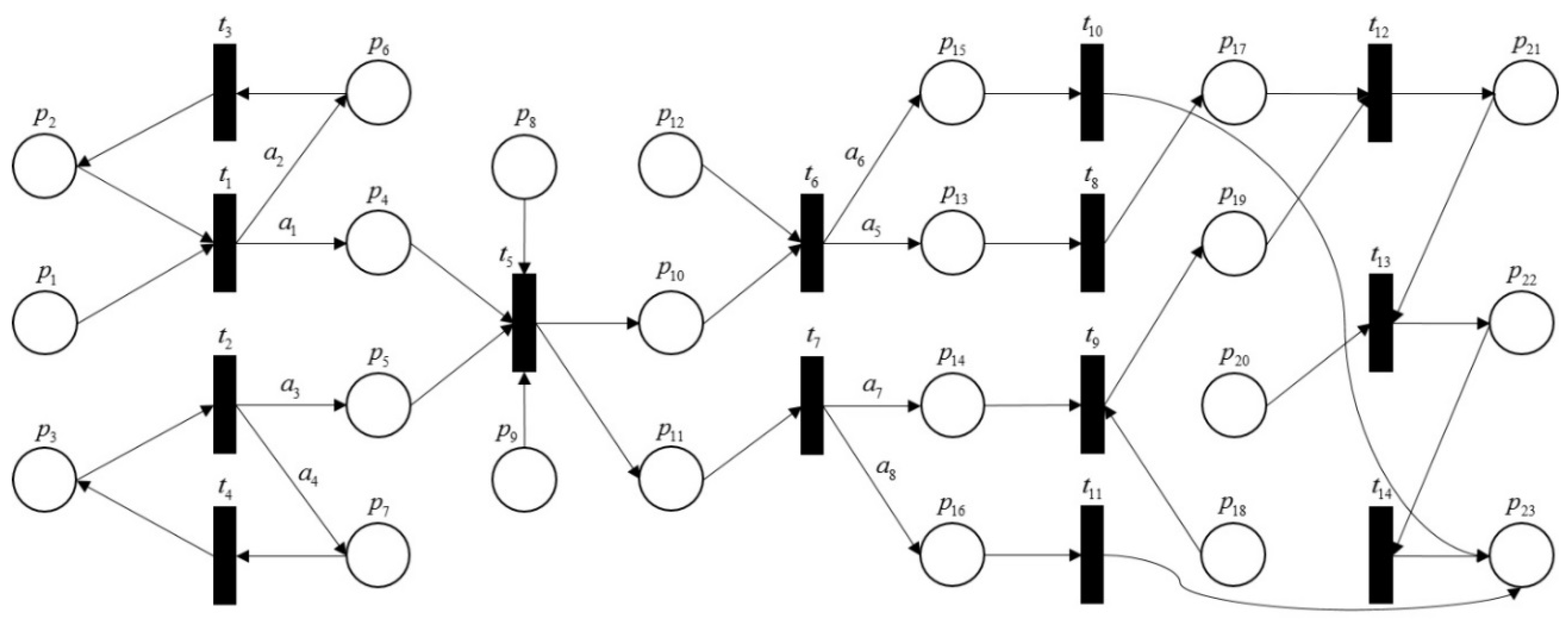
Based on the description of the production logistics problem, TCPN is used to model production and logistics in an FMS. The TCPN model of the self-adaptive collaboration method is established as shown in Figure 3.

In the TCPN model, the meaning of each transition has been briefly explained in

Table 1. Transitions in Figure 3.

Transition	Description of Transitions
$t_1$	The transition aims at modeling the check of the worker
$t_2$	The transition aims at modeling the check of the material
$t_3$	The transition aims at modeling requesting the worker
$t_4$	The transition aims at modeling requesting the material
$t_5$	The transition aims at modeling the machine processing and publishing a logistics task
$t_6$	The transition aims at modeling the quality detection
$t_7$	The transition aims at modeling the selection of the AGV
$t_8$	The transition aims at modeling the temporary storage
$t_9$	The transition aims at modeling the selected AGV going to the start point
$t_{10}$	The transition aims at modeling the reprocessing or the scarp
$t_{11}$	The transition aims at modeling the rejection of the AGV
$t_{12}$	The transition aims at modeling picking pallet and loading
$t_{13}$	The transition aims at modeling the selected AGV going to the destination
$t_{14}$	The transition aims at modeling the unloading

.

Table 2. Places in Figure 3. WIP: work in process.

Place	Description of Places
$p_1$	A token in this place represents a production task
$p_2$	A token in this place represents a worker
$p_3$	A token in this place represents a material
$p_4$	A token in this place represents the attendance of the worker
$p_5$	A token in this place represents enough materials
$p_6$	A token in this place represents the absence of the worker
$p_7$	A token in this place represents insufficient materials
$p_8$	A token in this place represents the sataus information of a machine
$p_9$	A token in this place represents the sataus information of an AGV
$p_{10}$	A token in this place represents the finish of the machine processing
$p_{11}$	A token in this place represents the request to the logistics task
$p_{12}$	A token in this place represents the detection result
$p_{13}$	A token in this place represents the qualified WIP
$p_{14}$	A token in this place represents the nearest and available AGV
$p_{15}$	A token in this place represents the unqualified WIP
$p_{16}$	A token in this place represents the remote or unavailable AGV
$p_{17}$	A token in this place represents an out-buffer
$p_{18}$	A token in this place represents the selected logistics task
$p_{19}$	A token in this place represents the correct start point
$p_{20}$	A token in this place represents the transport time
$p_{21}$	A token in this place represents the transport to the destination
$p_{22}$	A token in this place represents the correct destination
$p_{23}$	A token in this place represents the end and next cycle

explains the meaning of each place. The global color set declarations are given in

Table 3. Global color set declarations.

Color Set	Place
colset UNIT = unit; colset INT = int; colset REAL = real; colset STRING = string;
colset MIDxWIDxMAIDxNUMxT = product STRING*STRING*STRING*REAL*REAL timed;	$p_1$
colset MIDxMAIDxNUMxT = product STRING*STRING*REAL*REAL timed;	$p_3$, $p_5$, $p_7$, $p_{10}$, $p_{13}$, $p_{15}$, $p_{17}$
colset MIDxWIDxT = product STRING*STRING*REAL timed;	$p_2$, $p_4$, $p_6$
colset MIDxMAIDxNUMxPT = product STRING*STRING*REAL*REAL timed;	$p_8$
colset AIDxLOCxRSxT = product STRING*STRING*REAL*REAL timed;	$p_9$, $p_{14}$, $p_{16}$
colset AIDxLOCxRSxNUMxT = product STRING*STRING*REAL*REAL*REAL timed;	$p_{11}$
colset Q = string;	$p_{12}$
colset SPxDES = product STRING*STRING;	$p_{18}$
colset AIDxSPxDESxT = product STRING*STRING*STRING*REAL timed;	$p_{19}$, $p_{21}$, $p_{22}$, $p_{23}$
colset TT = real;	$p_{20}$
var MID,WID,MAID,AID,LOC,Q,SP,DES: STRING; var T,NUM,PT,RS,TT: REAL;

.

Figure 3 shows the TCPN model of the self-adaptive collaboration method. This model refers to the basic cycle of production-logistics systems, which consists of twenty-three places and fourteen transitions. Conditional statement expressions are assigned to the directed arcs $a_1$, $a_2$, $a_3$, $a_4$, $a_5$, $a_6$, $a_7$, and $a_8$. The cycle starts with checking workers and materials to be processed in production cells. Transition $t_1$ denotes the check of workers while transition $t_2$ denotes the check of materials. If the workers or materials are not ready, they will be requested. Otherwise, the materials will be processed on the machine. Transition $t_5$ describes machine processing as well as publishing a logistics task. The two processes are performed at the same time. The remaining time of the current operation of the machine is calculated and considered as a critical parameter for selecting an AGV. While a logistics task is published, all AGVs actively request the task. A token in the place $p_9$ represents the status information of an AGV, including current location and remaining space, which are collected by embedded devices or sensors. Thus, the machine can perceive the status of the AGV. Transition $t_6$ represents the quality detection of the WIP after machine processing. Unqualified WIP will be reprocessed or abandoned based on the detection standards. Transition $t_{10}$ denotes the reprocessing or the scarp. If the WIP is unqualified and needs to be reprocessed or abandoned, this cycle ends and the next cycle begins. Only the qualified one will be sent to the out-buffer of the production cell and wait to be transported to the next production cell. Transition $t_7$ represents selection of an AGV. The nearest AGV with remaining space will be selected as one of the feasible options. Based on the current tasks and routes, the selected AGV will decide whether to accept the logistics task or not. Finally, the most appropriate AGV will be selected to finish the logistics task. $t_9$ and $t_{12}$ represent that the AGV goes to the out-buffer and then picks and loads the pallet which carries the WIP. $t_{13}$ and $t_{14}$ represent that the AGV goes to the destination and unloads the pallet on the in-buffer of the next production cell. After the selected AGVs have finished their deliveries, the smart machine will select the nearest AGVs with enough remaining space to conduct the transportation of other jobs. Then, this cycle ends and next cycle begins.

3.3. Mechanism of Self-Adaptive Collaboration

In this part, based on the depiction of the proposed TCPN model, the mechanism of self-adaptive collaboration for production-logistics systems is investigated. The objective of the proposed TCPN model is to minimize the waiting time of all jobs, the makespan, and the electricity consumption of all machines and AGVs. Three KPIs including waiting time, makespan, and electricity consumption are considered.

The KPI waiting time is used to calculate the total waiting time of all jobs. The waiting time represents the time between two sequential operations of the same job. The total waiting time of all jobs is mathematically formulated to minimize the objective $\Delta T_{total}$ as follows:

$$\mathrm{Minimize} \Delta T_{total}={\displaystyle \sum _{i=1}^{m-1}{\displaystyle \sum _{h=2}^m{\displaystyle \sum _{j=1}^n\Delta T_{ihj}}}}$$

(1)

$$\mathrm{where} \Delta T_{ihj}=\Delta T_{ij}^{WA}+\Delta T_{ihk}^A+\Delta T_{hj}^{WB},\text{ for all }\left(i,j\right)\to \left(h,j\right)$$

(2)

In Equations (1) and (2), the waiting time $\Delta T_{ihj}$ is composed of three parts, namely the waiting time after processing $\Delta T_{ij}^{WA}$, the transport time $\Delta T_{ihk}^A$, and the waiting time before processing $\Delta T_{hj}^{WB}$. $\Delta T_{ij}^{WA}$ can be reduced by calling for AGVs once the job $j$ begins being processed on machine $i$. The transport time refers to the time cost of transporting materials between machines. $\Delta T_{ihk}^A$ can be reduced by selecting the nearest available AGV and planning a time-saving route. $\Delta T_{hj}^{WB}$ is influenced by the former two parts and is related to the production schedule.

The KPI makespan is used to calculate the maximum completion time of all jobs. The makespan is mathematically formulated to minimize the objective $C_{\max }$ as follows:

$$\mathrm{Minimize} C_{\max }=\underset{j}{\max }{C}_j$$

(3)

$$\mathrm{where} C_j=y_{1j}+{\displaystyle \sum _{i=1}^m{p}_{ij}+{\displaystyle \sum _{i=1}^{m-1}{\displaystyle \sum _{h=2}^m\Delta T_{ihj}}}},\text{ for all }\left(i,j\right)\to \left(h,j\right)$$

(4)

In Equations (3) and (4), $C_j$ denotes the completion time of the job $j$, $y_{1j}$ denotes the starting time of the first operation of the job $j$, ${\displaystyle \sum _{i=1}^m{p}_{ij}}$ denotes the processing time of the job $j$, and ${\displaystyle \sum _{i=1}^{m-1}{\displaystyle \sum _{h=2}^m\Delta T_{ihj}}}$ denotes the total waiting time of the job $j$. To reduce the makespan, the processing sequence or the processing speed of machines can be adjusted based on realities of the situation.

The KPI electricity consumption is used to calculate the total electricity consumption of all machine tools and AGVs. The total electricity consumption is mathematically formulated to minimize the objective $E_{total}$ as follows:

$$\mathrm{Minimize} E_{total}={\displaystyle \sum _{i=1}^m{E}_M^{(i)}}+{\displaystyle \sum _{k=1}^w{E}_{AGV}^{(k)}}$$

(5)

$$\mathrm{where} E_M^{(i)}={\displaystyle {\int }_0^t{P}_M^{(i)}(t)\mathrm{d}t}, P_M^{(i)}=P_{MP}^{(i)}\text{ when processing}, P_M^{(i)}=P_{MI}^{(i)}\text{ when idle}$$

(6)

$$E_{AGV}^{(k)}={\displaystyle {\int }_0^t{P}_{AGV}^{(k)}}(t)\mathrm{d}t$$

(7)

In Equations (5)–(7), $E_M^{(i)}$ denotes the electricity consumption of machine $i$, $E_{AGV}^{(k)}$ denotes the electricity consumption of AGV $j$, $P_M^{(i)}$ denotes the power of the machine $i$, $P_{MP}^{(i)}$ denotes the average power of the machine $i$ when processing, $P_{MI}^{(i)}$ denotes the average power of the machine $i$ when idle, and $P_{AGV}^{(k)}$ denotes the average power of AGV $k$. To reduce the total electricity consumption, the running time of all machines and AGVs should be shortened.

In the proposed TCPN model, the smart machine can calculate the remaining time of current operations. The remaining time of operation $\left(i,j\right)$ can be formulated as follows.

$$\Delta T_{ij}^R=\max \left\{0,C_{ij}-t\right\}$$

(8)

where $\Delta T_{ij}^R$ denotes the remaining time of operation $\left(i,j\right)$, $C_{ij}$ denotes the completion time of operation $\left(i,j\right)$, and $t$ denotes the current time.

While the machine processing begins, the smart machine actively publishes a logistics task for the WIP being processed. All AGVs actively request the logistics task and provide with real-time status information, such as current location and remaining space. The smart machine will select AGVs which are nearest and have enough remaining space. For example, if an available AGV can arrive at the smart machine within the remaining time of current operation, the waiting time of the operation after processing will be reduced to 0. The optimization of matches between logistics tasks and AGVs can be formulated as follows.

$$\mathrm{Minimize} {\displaystyle \sum _{i=1}^m{\displaystyle \sum _{k=1}^w{\left(T_{ik}-\Delta T_{ij}^R\right)}^2}}$$

(9)

$$\mathrm{where} Q_{ih}\le Q_k^A(t)$$

(10)

In Equations (9) and (10), $T_{ik}$ denotes the time cost of AGV $k$ arriving at the machine $i$, $\Delta T_{ij}^R$ denotes the remaining time of operation $\left(i,j\right)$, $Q_{ih}$ denotes the volume of WIP transported from machine $i$ to machine $h$, and $Q_k^A(t)$ denotes the remaining space of AGV $k$ at the current time $t$.

While a logistics task is published, the smart AGV will actively request the task. If several machines choose a smart AGV simultaneously, the smart AGV makes a decision based on the priority of these tasks as well as the remaining space. The priority of tasks can be formulated as follows:

$$P_{ihj}=y_{hj}-t,\text{ for all }\left(i,j\right)\to \left(h,j\right)$$

(11)

where $P_{ihj}$ denotes the priority of logistics task between operation $\left(i,j\right)$ and operation $\left(h,j\right)$, $y_{hj}$ denotes the starting time of operation $\left(h,j\right)$, and $t$ denotes the current time. Based on the proposed priority, the logistics task can be categorized into two types, namely the urgent logistics task and the normal logistics task. If $P_{ihj}<0$, then the task is an urgent task. Otherwise, the task is a normal task. For the urgent logistics task, the next machine is idle and waiting for the task. For the normal logistics task, the next machine is not available and the WIP being transported has to wait in a list. The smart AGV will select logistics tasks that have the highest priority and the volume of tasks must be less than the remaining space of the AGV. Then, the smart AGV can compute the time cost of feasible routes to go to the start point and transport the WIP to the destination. The time cost $T_{ik}$ for AGV $k$ arriving at the machine $i$ can be formulated as follows:

$$T_{ik}={\displaystyle \sum _{r=1}^n{T}_{ik}^{(r)}(t)}$$

(12)

$$\mathrm{where} T_{ik}^{(r)}(t)=L_r/v_k(t)$$

(13)

In Equations (12) and (13), $T_{ik}^{(r)}(t)$ denotes the time cost of AGV $k$ passing road segment $r$ at current time $t$, $L_r$ denotes the path length of the road segment $r$, and $v_k(t)$ denotes the current speed of AGV $k$. Thus, a feasible route with the least time cost will be selected as the optimal route. The optimization of routes selection is implemented constantly during the transport and in real time.

In this paper, based on the real-time status information of machines, AGVs, and WIP, the objective functions are implemented in the application layer of the cloud service platform and the results are input into the TCPN model through the colored tokens located in the places.

4. Simulation Results

This section introduced an industrial case from an engine manufacturing company in Xi’an. In the case company, FMS was used to manage and coordinate key equipment and automatize the production. Engine components were processed on different machines in the given processing sequence. A material handling system was used to transport these components between machines. However, the machining environment changed dynamically due to the external and internal fluctuations, and the optimal process plan and schedule became less efficient or even infeasible. Thus, the case company needed production-logistic collaboration methods and tools to solve the problems. Based on the investigation of the case company, a simulation experiment was conducted in the laboratory by using CPN Tools to validate the performance and applicability of the proposed method.

In the simulation experiment, an instance of job shop problems from [25] was used as a feasible schedule plan, including four machines and three jobs, as shown in

Table 4. The instance of the job shop problem.

Jobs	Machine Sequence	Processing Times	Volume
1	1, 2, 3	$p_{11}=10,p_{21}=8,p_{31}=4$	1
2	2, 1, 4, 3	$p_{22}=8,p_{12}=3,p_{42}=5,p_{32}=6$	2
3	1, 2, 4	$p_{13}=4,p_{23}=7,p_{43}=3$	1.5

. $p_{ij}$ denotes the processing time of the operation that job $j$ is processed on machine $i$, $i=1,2,3,4,j=1,2,3$. These jobs would be processed by a list of machines in a given order. The volume of each job was given in Table 4 because the volume capacity of AGVs was considered as a constraint in the simulation experiment. A feasible schedule plan is shown Figure 4. The initial time of the schedule was 0. The gray segment represented the variable waiting time between two continuous operations of the same job. In addition, two AGVs were added in the simulation experiment in order to investigate the collaborative relationship between production and logistics in a job shop.

Thus, the aforementioned job shop consisted of the following main components, namely a warehouse, four production cells, and two AGVs. The warehouse had an in-buffer and an out-buffer. Each production cell had a machine, an in-buffer, and an out-buffer. Machines and AGVs installed with sensors had the capability of perceiving status information in real time and making decisions based on the knowledge base and real-time information. Other manufacturing resources, such as in-buffers, out-buffers, pallets, and WIP were attached RFID tags to provide real-time location information. The workers had staff cards with embedded RFID tags to provide individual information.

For simplicity of understanding but without losing generality of principle, some initial and basic information of manufacturing resources were given as follows. The average power of each machine when processing was 15, while the average power of each machine when idle was 4. AGV1 and AGV2 had the same initial location (0, 4.5). The average power of each AGV was 7. The speed of each AGV was 5 and the maximum space of each AGV was 3. The production and logistics began at initial time 0. Firstly, raw materials were transported to smart machines by smart AGVs. Then, the machine processing started and smart machines actively published logistics tasks. Next, smart AGVs actively requested the logistics tasks. The layout of the shop floor is shown in Figure 5. The black spots in the layout represented the location of in-buffers or out-buffers of the warehouse or production cells.

As shown in Figure 5, a simulation experiment was conducted based on the case scenario. In the experiment, a personal computer, fifteen antennas, four RFID readers, and nine RFID tags were used. Antennas were connected to readers and readers were connected to the computer. The RFID tags were attached to different manufacturing objects, such as machines, AGVs, and WIP. Antennas were used to collect real-time status information of these manufacturing objects from attached RFID tags.

Computational experiments were conducted by R-3.3.0 for Windows (64-bit) in a PC with a quad-core AMD A10-5750M processor at 2.5 GHz and 8 GB DDR3-1333 RAM. R-3.3.0 for Windows (64-bit) is a software environment for statistical computing and graphics. Referring to the manufacturing process, the TCPN model was built up in CPN Tools, as shown in Figure 5. The TCPN model started running at the same time when the production and logistics were executed according to the planned time. Firstly, real-time status information of machines, AGVs, and WIP were transmitted to the PC through RFID reader ports. Secondly, based on the collected information, the objective functions were implemented by R-3.3.0 for Windows (64-bit) in the PC and the results were stored in Standard ML (SML) files. Thirdly, every time the cycle of the TCPN model started, the information in the SML files was updated. By loading SML files, the status of colored tokens was tuned accordingly.

Using the proposed method, the simulation result is shown in

Table 5. The result of the simulation experiment.

Task ID	Start Point (X, Y)	Destination (X, Y)	Job ID	Priority	AGV ID	Remaining Space	Waiting Time			Computing Time (s)
							After	Transport	Before
T0001	W(0, 4.5)	M1(2.5, 4.5)	1	0-t	A001	2	0	0.5	0	<0.01
T0002	W(0, 4.5)	M2(2.5, 2)	2	0-t	A002	1	0	1	0	<0.01
T0003	W(0, 4.5)	M1(2.5, 4.5)	3	10-t	A001	0.5	0	0.5	10	<0.01
T0004	M1(5.5, 3)	M2(2.5, 2)	1	10-t	A002	2	0	0.8	0	<0.01
T0005	M2(5.5, 0.5)	M1(2.5, 4.5)	2	14-t	A002	1	4.1	1.4	0	<0.01
T0006	M1(5.5, 3)	M4(6.5, 2)	2	17-t	A002	1	0	0.4	0	<0.01
T0007	M1(5.5, 3)	M2(2.5., 2)	3	18-t	A001	1.5	4	0.8	0	<0.01
T0008	M2(5.5, 0.5)	M3(6.5., 4.5)	1	18-t	A002	2	0	1	0	<0.01
T0009	M4(9.5, 0.5)	M3(6.5., 4.5)	2	22-t	A002	1	0	1.4	0	<0.01
T0010	M2(5.5, 0.5)	M4(6.5., 2)	3	25-t	A001	1.5	0	0.5	0	<0.01

. T0001 denotes the first published logistics task, W denotes the warehouse, M1 denotes the machine1, A001 denotes the AGV1, and similarly for the others. The total waiting time was 26.4. The makespan was 30.3. The electricity consumption of machines was 894.8, while the electricity consumption of AGVs was 98.7. Thus, the total electricity consumption was 993.5. The efficiency of the proposed model was verified and the result showed that the computing time was less than 0.01 s, which was reasonable for implementing the proposed method in the real manufacturing environment.

A comparative study between an event-driven method [18] and the proposed TCPN based self-adaptive collaboration method was presented. Since real-life data were not given in the paper used for the comparative study, an instance of job shop problems from [25] was used as a feasible schedule plan, including four machines and three jobs, as shown in Table 4. Based on the same benchmark, the objective functions were implemented by R-3.3.0 for Windows (64-bit) in the PC with the consideration of three KPIs including waiting time, makespan, and electricity consumption. The result of the comparative study is shown in

Table 6. The result of the comparative study. KPI: key performance indicators.

KPI	Event-Driven Method	Self-Adaptive Collaboration Method
Total waiting time	37.1	26.4
Makespan	36.3	30.3
Total electricity consumption	1035.3	993.5

. The result demonstrated that the TCPN-based self-adaptive collaboration method outperformed the event-driven method in reductions of waiting time, makespan, and electricity consumption.

5. Conclusions

This work contributes to the study of production-logistics collaboration to improve economic and environmental performances of production-logistics systems. A TCPN simulation-based self-adaptive collaboration method for production-logistics systems is proposed. The method combines the schedule of token sequences in the timed colored Petri net with real-time status of key production and logistics equipment. The key equipment is made ‘smart’ to actively publish or request logistics tasks. An integrated framework based on cloud service platform is introduced to provide the foundations for self-adaptive collaboration of production-logistics systems. The capabilities of key equipment are packaged as cloud services to be published on the cloud services platform. Computational experiments demonstrate that the proposed method is feasible and effective in reducing waiting time, makespan, and electricity consumption. A comparative study is implemented and the result indicates that the proposed method outperforms the event-driven method in improving the overall efficiency of the production-logistics systems and reducing electricity consumption. This work can be applied to other types of manufacturing systems to implement production-logistics collaboration. Future research will mainly focus on the following aspects. Other algorithms would be investigated and used to develop the production-logistics collaboration model and real-life data from the manufacturing environment would be used to verify the production-logistics collaboration model.

References

1. Herrero, D.; Mart, H. Modeling Distributed Transportation Systems Composed of Flexible Automated Guided Vehicles in Flexible Manufacturing Systems. IEEE Trans. Ind. Inform. 2010, 6, 166–180. [Google Scholar] [CrossRef]
2. Li, D.X.; He, W.; Li, S. Internet of Things in Industries: A Survey. IEEE Trans. Ind. Inform. 2014, 10, 2233–2243. [Google Scholar]
3. Xu, X. From cloud computing to cloud manufacturing. Robot. Comput. Integr. Manuf. 2012, 28, 75–86. [Google Scholar] [CrossRef]
4. Zhang, Y.; Qian, C.; Lv, J.; Liu, Y. Agent and cyber-physical system based self-organizing and self-adaptive intelligent shopfloor. IEEE Trans. Ind. Inform. 2017, in press. [Google Scholar] [CrossRef]
5. Girbea, A.; Suciu, C.; Nechifor, S.; Sisak, F. Design and implementation of a service-oriented architecture for the optimization of industrial applications. IEEE Trans. Ind. Inform. 2014, 10, 185–196. [Google Scholar] [CrossRef]
6. Zhang, Y.F.; Ren, S.; Liu, Y.; Si, S.B. Big data based analysis architecture of complex product manufacturing and maintenance process for sustainable production. J. Clean. Prod. 2017, 142, 626–641. [Google Scholar] [CrossRef]
7. Zhang, Y.; Zhang, G.; Wang, J.; Sun, S.; Si, S.; Yang, T. Real-time information capturing and integration framework of the internet of manufacturing things. Int. J. Comput. Integr. Manuf. 2015, 28, 811–822. [Google Scholar] [CrossRef]
8. Li, X.; Song, J.; Huang, B. A scientific workflow management system architecture and its scheduling based on cloud service platform for manufacturing big data analytics. Int. J. Adv. Manuf. Technol. 2016, 84, 119–131. [Google Scholar] [CrossRef]
9. Um, I.; Cheon, H.; Lee, H. The simulation design and analysis of a flexible manufacturing system with automated guided vehicle system. J. Manuf. Syst. 2009, 28, 115–122. [Google Scholar] [CrossRef]
10. Uzam, M.; Zhou, M. An Iterative Synthesis Approach to Petri Net-Based Deadlock Prevention Policy for Flexible Manufacturing Systems. IEEE Trans. Syst. Man Cybern. A Syst. Hum. 2007, 37, 362–371. [Google Scholar] [CrossRef]
11. Li, Z.W.; Zhou, M.C.; Wu, N.Q. A survey and comparison of Petri net-based deadlock prevention policies for flexible manufacturing systems. IEEE Trans. Syst. Man Cybern. C Appl. Rev. 2008, 38, 173–188. [Google Scholar]
12. Silva, M. Individuals, Populations and fluid approximations: A Petri net based perspective. Nonlinear Anal. Hybrid Syst. 2016, 22, 72–97. [Google Scholar] [CrossRef]
13. Wang, S.; You, D.; Wang, C. Optimal supervisor synthesis for petri nets with uncontrollable transitions: A bottom-up algorithm. Inf. Sci. 2016, 363, 261–273. [Google Scholar] [CrossRef]
14. Baruwa, O.T.; Piera, M.A. A coloured Petri net-based hybrid heuristic search approach to simultaneous scheduling of machines and automated guided vehicles. Int. J. Prod. Res. 2016, 54, 4773–4792. [Google Scholar] [CrossRef]
15. Raj, J.A.; Ravindran, D.; Saravanan, M.; Prabaharan, T. Simultaneous scheduling of machines and tools in multimachine flexible manufacturing systems using artificial immune system algorithm. Int. J. Comput. Integr. Manuf. 2014, 27, 401–414. [Google Scholar] [CrossRef]
16. Xia, H.; Li, X.; Gao, L. A hybrid genetic algorithm with variable neighborhood search for dynamic integrated process planning and scheduling. Comput. Ind. Eng. 2016, 102, 99–112. [Google Scholar] [CrossRef]
17. Lacomme, P.; Larabi, M.; Tchernev, N. Job-shop based framework for simultaneous scheduling of machines and automated guided vehicles. Int. J. Prod. Econ. 2013, 143, 24–34. [Google Scholar] [CrossRef]
18. Qu, T.; Lei, S.P.; Wang, Z.Z.; Nie, D.X.; Chen, X.; Huang, G.Q. IoT-based real-time production logistics synchronization system under smart cloud manufacturing. Int. J. Adv. Manuf. Technol. 2016, 84, 147–164. [Google Scholar] [CrossRef]
19. Luo, H.; Wang, K.; Kong, X.T.R.; Lu, S.; Qu, T. Synchronized production and logistics via ubiquitous computing technology. Robot. Comput. Integr. Manuf. 2017, 45, 99–115. [Google Scholar] [CrossRef]
20. Li, W.; Zhao, Y.; Lu, S.; Chen, D. Mechanisms and challenges on mobility-augmented service provisioning for mobile cloud computing. IEEE Commun. Mag. 2015, 53, 89–97. [Google Scholar] [CrossRef]
21. Lee, J.; Kim, Y.; Kwak, Y.; Zhang, J.; Papasakellariou, A.; Novlan, T.; Sun, C.; Li, Y. LTE-advanced in 3GPP Rel-13/14: An evolution toward 5G. IEEE Commun. Mag. 2016, 54, 36–42. [Google Scholar] [CrossRef]
22. Baruwa, O.T.; Piera, M.A.; Guasch, A. TIMSPAT—Reachability graph search-based optimization tool for colored Petri net-based scheduling. Comput. Ind. Eng. 2016, 101, 372–390. [Google Scholar] [CrossRef]
23. Baruwa, O.T.; Piera, M.A.; Guasch, A. Deadlock-Free Scheduling Method for Flexible Manufacturing Systems Based on Timed Colored Petri Nets and Anytime Heuristic Search. Int. J. Prod. Res. 2014, 45, 831–846. [Google Scholar] [CrossRef]
24. Jensen, K.; Kristensen, L.M. Formal Definition of Timed Coloured Petri Nets. In Coloured Petri Nets; Springer: Berlin/Heidelberg, Germany, 2009; pp. 257–271. [Google Scholar]
25. Pinedo, M.L. Machine Scheduling and Job Shop Scheduling. In Planning and Scheduling in Manufacturing and Services; Springer: New York, NY, USA, 2009; pp. 83–115. [Google Scholar]
Figure 1. An integrated framework based on cloud service platform for production-logistics systems. AGV: automated guided vehicle.
Applsci 07 00235 g001
Figure 2. The simplified schedule plan of a job.
Applsci 07 00235 g002
Figure 3. The timed colored Petri net model for self-adaptive collaborative production-logistics systems.
Applsci 07 00235 g003
Figure 4. The feasible schedule plan.
Applsci 07 00235 g004
Figure 5. Simulation experiment of the case scenario. CPN: colored Petri nets; RFID: radio frequency identification.
Applsci 07 00235 g005