Friction Factor Correlation for Regenerator Working in a Travelling-Wave Thermoacoustic System

Abstract

Regenerator is a porous solid structure which is important in the travelling-wave thermoacoustic system. It provides the necessary contact surface and thermal capacity for the working gas to undergo a thermodynamic cycle under acoustic oscillatory flow conditions. However, it also creates a pressure drop that could degrade the overall system performance. Ideally, in a travelling-wave system, the phase angle between oscillating pressure and velocity in the regenerator should be zero, or as close to zero as possible. In this study, the hydrodynamic condition of a regenerator has been investigated both experimentally (in a purpose-built rig providing a travelling-wave phasing) and numerically. A two-dimensional ANSYS FLUENT CFD model, capturing the important features of the experimental conditions, has been developed. The findings suggest that a steady-state correlation, commonly used in designing thermoacoustic systems, is applicable provided that the travelling-wave phase angle is maintained. However, for coarse mesh regenerators, the results show interesting “phase shifting” phenomena, which may limit the correlation validity. Current experimental and CFD studies are important for predicting the viscous losses in future models of thermoacoustic systems.

1. Introduction

The underlying mechanism of the thermoacoustic energy conversion processes is a heat transfer interaction taking place between the gas parcels undergoing oscillatory motion and a solid material along which the gas oscillations occur. In thermoacoustic prime movers (engines), a spontaneous acoustic wave is excited which causes the gas parcel oscillations coupled with their compression and expansion, thus providing a means of transporting heat from the hotter to the cooler place of the solid. In thermoacoustic coolers, the acoustically induced displacement/compression/expansion of gas parcels leads to heat pumping effects in the solid. The solid material used in such applications often takes the form of a porous structure—for example, stacked layers of woven mesh screens—which by analogy to classic Stirling engines is referred to as “regenerator”.

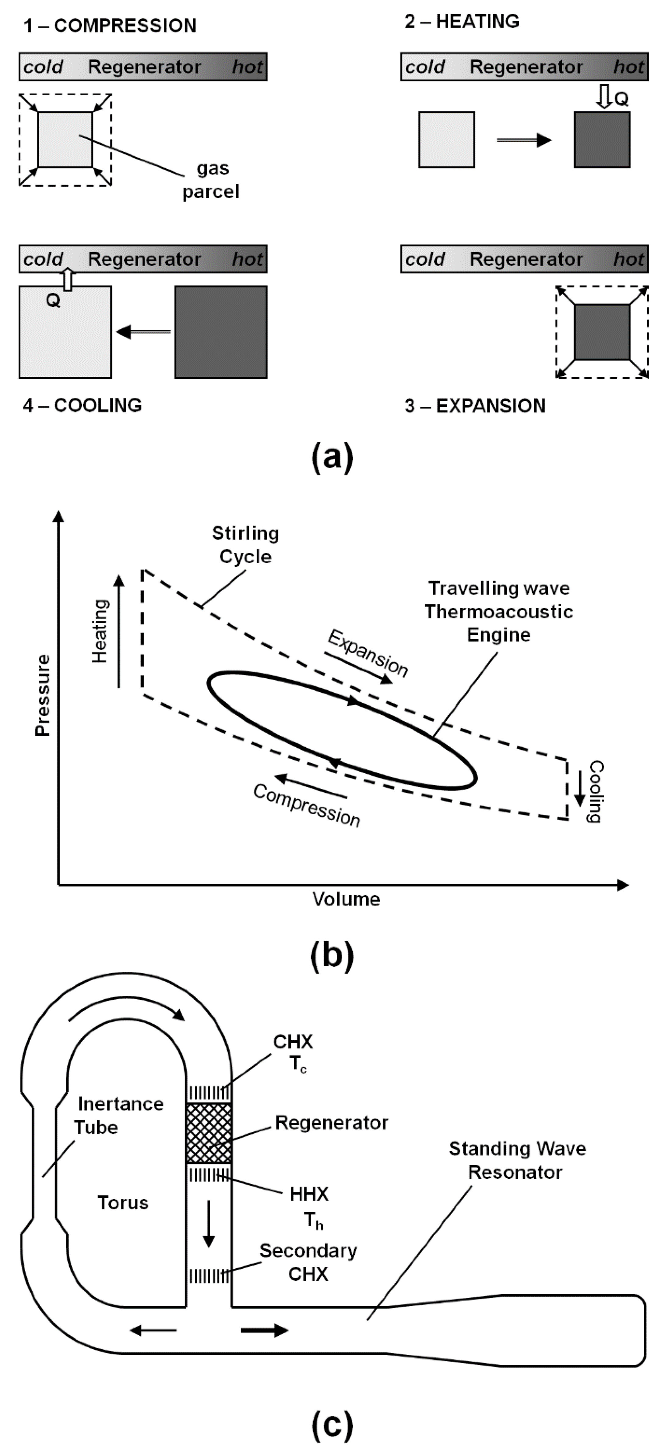
Figure 1a explains the interaction of gas parcels with a solid material (in this example, a plate with an imposed temperature gradient). The gas experiences thermal expansion during the displacement towards the higher temperature and thermal contraction during the displacement towards the lower temperature. In this way, the correct time phasing is obtained to meet the Rayleigh’s criterion [1] to produce power. Figure 1b illustrates the thermodynamic cycle in comparison to the classic ideal Stirling cycle, while Figure 1c shows one of the known configurations of thermoacoustic engines referred to as Thermo-Acoustic Stirling Heat Engine, TASHE [2].

Strictly speaking, the thermoacoustic core (a regenerator placed between the hot and cold heat exchangers) works simply as a power amplifier. To complete this Stirling-like thermodynamic process, acoustic power has to be fed to the ambient end of the regenerator with a near travelling-wave phasing. This leads to practical designs having feedback resonator types (closed loops) with various acoustic network elements such as inertance and compliance to control the correct/preferred phasing between pressure and velocity oscillation; further discussions are available in reference [3].

Thermoacoustic systems have gained considerable attention due to their environmental friendliness arising from the use of inert/noble gases as the working media and the lack of moving parts when executing the thermodynamic cycle which makes them of simple design and potentially of high reliability and low cost.

As part of the requirement to achieve high performance, the regenerator is used in travelling-wave thermoacoustic device with an aim to provide sufficient thermal contact with the working medium but also cause as little viscous loss as possible. Thermal contact is improved due to the large surface area of the porous and tortuous structure of the regenerator. However, care is needed to avoid high viscous losses. From the practical point of view, and to illustrate these problems, the regenerators are typically constructed from metal wire mesh screens by compacting a large number of wire mesh disks (tens or hundreds) along the direction of wave propagation. The conflict between efficient thermal contact and unwanted pressure losses of the porous and tortuous structure of the regenerator requires careful investigation. In the context of thermoacoustics, the matter is difficult to address not only because the oscillatory nature of the flow but also because the correctly defined phasing between pressure and velocity needs to be considered.

However, most of the past experiments have not considered specific phase angles between pressure and velocity oscillations. Therefore, their effect on the regenerator hydrodynamic condition is still unknown. This necessitates the development of an appropriate closure model for a regenerator working in the travelling-wave mode since a hydrodynamic correlation based on an unspecified phase angle may introduce unknown errors. Since the regenerators are porous media they can be studied theoretically on the grounds of the porous medium theory [4]. This allows modelling a porous structure through the use of additional parameters in the transport equation that represent the resistance to the flow.

Until now, the behaviour of the oscillatory flow across a porous medium is not fully understood. The matter is complicated further by the requirement of a specific phase angle between pressure and velocity for the thermoacoustic device to function properly. In addition, the lack of a well-defined friction correlation for oscillatory flow across porous medium complicates the determination of correct closure model for the purpose of numerical modelling. These issues are addressed in the current work by the application of a mixture of experimental and CFD approaches.

2. Literature Review

The friction factor is a dimensionless parameter used to represent the hydrodynamic condition of a flow across a structure. In oscillatory flow the friction factor is defined as [5]:

$$f_{osc}=\frac{X_{\Delta P}{d}_h}{\frac{1}{2}\rho X_{u_m}^2{L}_r}.$$

(1)

The terms $X_{\Delta P}$, $d_h$, $\rho$, $X_{u_m}$, and $L_r$ represent the amplitude of pressure drop, hydraulic diameter, gas density, amplitude of velocity and length of the regenerator, respectively. The subscript $u_m$ relates to the mean value taken between two measured points. The hydraulic diameter, d_h, is defined as [5]:

$$d_h=\frac{\varphi }{1-\varphi }{d}_w.$$

(2)

The value of porosity, $\varphi$, and the wire diameter, $d_w$, are usually supplied by the manufacturer of mesh screens. The experimentally measured pressure drop and velocity are used to calculate the friction factor. The results calculated through Equation (1) may be fitted with suitable correlation to represent the hydrodynamic condition of the flow investigated. The basic form of friction factor correlation is given by the standard two-parameter Ergun equation [6]:

$$f=\frac{a_1}{Re}+a_2,$$

(3)

where $a_1$ and $a_2$ are constants that fit the condition tested. Swift and Ward [7] showed that the two constants of Equation (3) can be represented by an equation for porosity defined as:

$$a_1=1268-3545\varphi +2544{\varphi }^2,$$

(4)

$$a_2=-2.82+10.7\varphi -8.6{\varphi }^2.$$

(5)

In their correlation, Swift and Ward [7] defined the Reynolds number by taking into consideration the simple harmonic oscillation in regenerator and expressed it as the first order amplitude of complex Reynolds number, $R{e}_d$, given by:

$$R{e}_d=\frac{4‹u_1›r_h{\rho }_m}{\mu },$$

(6)

where $‹u_1›$, $r_h$, ${\rho }_m$ and $\mu$ are the first order spatial average velocity, hydraulic radius, mean density and viscosity, respectively. Assuming a simple harmonic oscillation in the regenerator, their correlation based on Equations (3)–(5) is reported to fit well the steady experimental data of Kays and London [8]. This equation had been widely used in thermoacoustic community in conjunction with DeltaEC, design software for thermoacoustic devices [9]. The suitability of Swift and Ward’s equation for use in an oscillatory flow is however questionable because it is fitted to steady flow data.

A number of research works considered various specific formulations of equations for friction factor, including Gedeon and Wood [6], Ju et al. [10], Nam and Jeong [11] or Boroujerdi and Esmaeili [12]. These formulations are generally of the same form as the standard Ergun Equation (3), but are typically multiplied by a certain dimensionless modification factor. This is typically obtained through dimensional analysis, experiments, numerical simulations or their useful combination, and its presence highlights the important differences between oscillatory and steady flow conditions.

Another important parameter in an oscillatory flow is referred to as (acoustic) impedance. It is defined as a ratio between pressure and velocity of a flow. However, impedance is a complex number and so in addition to their amplitudes it also includes the phase difference between them [3]. In travelling wave systems, the phase difference between pressure and velocity can be controlled by an RLC network which is also known in some papers as a “phase shifter”. Liu et al. [13] reported that the phase shifter reduces losses within the regenerator and improves system performance. This indicates that the pressure drop characteristics within the regenerator depend on the phase shift between pressure and velocity. In most of the papers discussed above, the phase difference between pressure and velocity is not set experimentally to a specific value. This may introduce additional unknown effects. There is yet no clear explanation as to how this affects the friction losses of the whole system. It is found, however, that several situations have been reported in the literature where the meaning of friction factor is unclear when the phase difference is present.

Hsu [14] showed that when a phase difference exists, setting the amplitude alone is not sufficient to predict the hydrodynamics of flow in the porous medium. The experimental detail is reported by Hsu et al. [15]. The coefficients $a_1$ and $a_2$ of the friction correlation (Equation (3)) are presented by Hsu et al. [15] as Darcy and Forchheimer coefficients. The friction factor gained from experimental results is discussed from a theoretical point of view. The theoretical explanation involves Stokes drag force, $C_s$, frictional force due to boundary layer, $C_B$, and inviscid form drag, $C_I$, first defined by Hsu and Cheng [16] and further developed theoretically by Hsu [14]. The theoretical prediction in that study is in good agreement with experimental results when the effect of phase difference is considered. In this paper, the phase difference between pressure and velocity will be referred to as “phase shifting” for brevity.

The findings of Hsu [14] may be related to the “phase shifting” phenomena reported by Ju et al. [10] and the breathing factor, $B$, introduced by Nam and Jeong [11]. The phase shift effect is also observed in the experimental study of Zhao and Cheng [17] when the kinetic Reynolds number increases with frequency. Clearly the phase shifting between pressure and velocity has an effect on friction losses reported in many investigations of oscillatory flows. There is a possibility that these phenomena occur as a result of the experimental conditions not being set to a particular time-phasing between pressure and velocity. However, no attention has been given to the possibility of controlling the time-phase between pressure and velocity in the experimentation for determination of the hydrodynamic condition of the oscillating flow through a regenerator. This is crucial in thermoacoustic applications because the regenerator should work with a well-controlled travelling-wave time-phasing.

The porous and tortuous structure of the regenerator is difficult and computationally very expensive to model using CFD if the full original structure is to be replicated. An economical way of modelling such a structure is through the use of the porous medium theory.

The porous medium theory models a porous structure through the use of additional parameters in the transport equation that represent the flow resistivity. Flow resistance is modelled through the knowledge of pressure drop caused by the structure. According to the Darcy–Forchheimer model, the pressure gradient, $\nabla p$, is defined as [4]:

$$\nabla p=-\frac{\mu }{K}v-F{K}^{-1/2}\rho \left|v\right|v,$$

(7)

where $\mu$, $\rho$, and $v$ are the gas dynamic viscosity, density and velocity, respectively. The terms $K$ and $F$ represent the additional parameters representing form drag to the flow and the terms are known as permeability coefficient and Forchheimer inertial coefficient, respectively. In the simplest case, the flow across the porous medium can be represented by Darcy’s law. Darcy’s law simply neglects the second term on the right hand side of Equation (7) leaving only the term with permeability coefficient, $K$, to represent the porosity experienced by the flow. This law is valid only when the Reynolds number, defined by the average flow velocity, is an order of magnitude smaller than one. When the velocity is high, the Forchheimer modified equation should be considered to account for the inertial losses in the porous medium. In this condition, Equation (7) should be applied in full. In a highly viscous flow, a further modification is suggested where the second term on the right hand side of Equation (7) is replaced with the Brinkman’s term, $K{\nabla }^{2}v$.

Darcy’s permeability, $K$, and Forchheimer inertial coefficient, $F$, are empirical constants. As empirical constants, both permeability and inertial coefficient are uniquely dependent on the porosity and tortuousity of the porous structure (regenerator). The values determine the momentum losses occurring in the porous media. In experimental practice, the momentum loss can be obtained from the pressure drop measured across the regenerator. On the other hand, to model a system with regenerator, one will need to determine the permeability, $K$, and Forchheimer inertial coefficient, $F$, beforehand. This becomes a challenge especially due to the lack of friction factor correlations suitable for oscillating flows in porous media.

Cha et al. [18] reported a CFD-assisted method for determining the permeability and inertial coefficient of a porous regenerator in an oscillating flow. The regenerator in their study, limited to a few sizes of mesh screens, is tested in a small sized device where the inertial effect could be significant. The oscillating flow friction factor is shown to deviate from the steady flow data of Clearman et al. [19] when the permeability Reynolds number, $R{e}_K=\rho u{K}^{1/2}/\mu$, is greater than 0.1. Landrum et al. [20] followed the same CFD procedure in establishing the hydrodynamic properties of the regenerator in an oscillating flow but with small mesh fillers suitable for miniature cryocoolers. In a different study, the porous medium coefficients were also derived by Tao et al. [21]. However, the derived equation is inappropriate for general use as the friction factor applied in defining the pressure drop is the equation specifically built for cryogenic conditions.

3. Experimental Setup

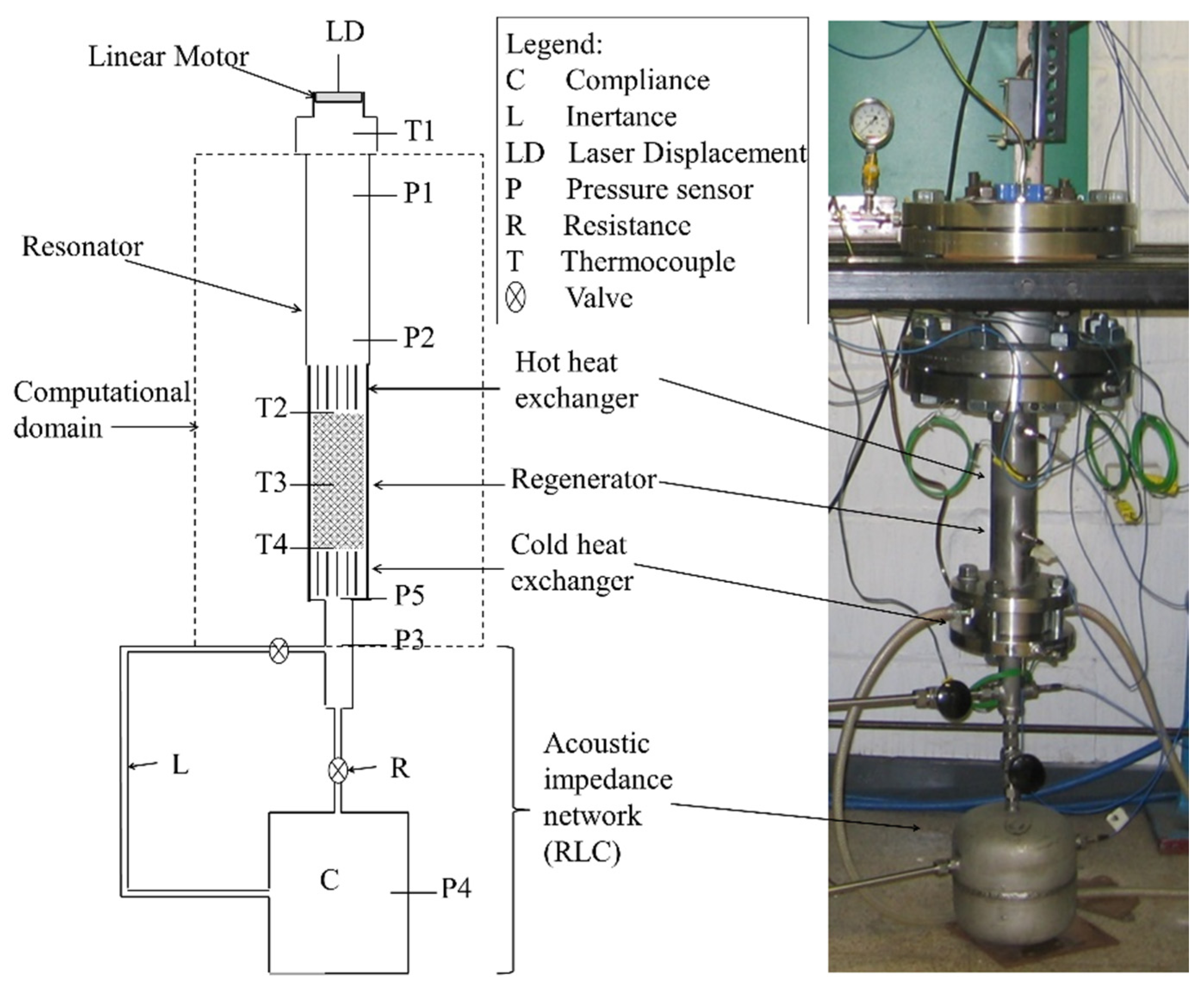
The schematic diagram of the test rig is shown in Figure 2. In essence, it is a travelling-wave cooler in which a sample of regenerator material can be placed and the resulting pressure drop is measured. The rig consists of a linear motor, resonator, hot and cold heat exchanger, regenerator (mesh numbers #30, #94, #180, and #200 have been used) and a set of components known as resistance, $R$, inertance, $L$, and compliance, $C$ (forming an RLC network). The network is a combination of suitable valves, a 1.6 m long tube with a diameter of 8 mm and a buffer volume of 2.5 × 10⁻³ m³. The frequency of the acoustic wave is set using a linear motor. The linear motor is enclosed in a specially designed high-pressure cylindrical casing with a glass window to allow laser displacement measurement of the motor piston. The laser displacement sensor (Keyence LK-G152, Milton Keynes, UK) senses the piston displacement, $\delta$. The amplitude of the velocity at that location, defined as $V_1$, is then calculated as $V_1=\omega \delta$.

The resonator has the inner diameter of 55 mm. The hot heat exchanger, regenerator and cold heat exchanger are made to fit into the resonator. The lengths of the resonator, hot heat exchanger, regenerator and cold heat exchanger are 185 mm, 25 mm, 50 mm and 27 mm, respectively. The regenerator is built using stainless steel mesh screens stacked on top of one another to fill up the 50 mm length. The supplied acoustic wave creates a temperature gradient along the regenerator. The development of the temperature gradient is controlled to concentrate only on the hydrodynamic condition of the regenerator. This is achieved through the cold heat exchanger located at the bottom end of the regenerator. The cold heat exchanger is connected to a reservoir that supplies water at room temperature so as it is kept at room temperature. The temperatures at locations T1, T2, T3 and T4 are measured by type-K thermocouples. The rig typically operates with helium at mean pressure up to 60 bar.

3.1. Data Collection and Reduction

The phase angle between pressure and velocity is controlled via the RLC network as shown in Figure 2. The valves are adjusted accordingly until the travelling-wave condition is achieved. The phase is observed by monitoring the phase angle, $\phi$, of impedance at location 5. The impedance at location 5, $Z_5$, is given as:

$$Z_5=\frac{P_5}{u_5}=\left|Z_5\right|\left(\cos \phi +i\sin \phi \right).$$

(8)

The terms$P_5$, $u_5$, and$\phi$ represent the oscillating pressure, oscillating velocity and phase angle of impedance at location P5, respectively. The phase angle of impedance represents the phase difference between pressure and velocity at that location. When the phase angle of impedance is zero, the imaginary part of impedance becomes zero. Hence oscillating pressure and oscillating velocity are both contributing only to the real value of impedance. As a result, pressure and velocity are in phase [22]. Pressures are measured in the experiment. The velocity at location 5, $u_5$, is determined using a Transfer Matrix Method. The Transfer Matrix Method has originally been used to measure the acoustical properties of components such as the porous media in the study by Song and Bolton [23] and Ueda et al. [24]. Ueda et al. [24] applied a linear thermoacoustic theory to estimate acoustic characteristics of a regenerator. In the current study, the method is used to theoretically provide information on variables not measured in the experiment. Lossless thermoacoustic model is used to relate pressure, $P$, and velocity, $u$, at two locations. This is shown in a matrix form as follows:

$$\left[\begin{array}{c}\frac{\partial P}{\partial x}\\ \frac{\partial u}{\partial x}\end{array}\right]=\left[\begin{array}{cc}0& -i\omega {\rho }_m\\ \frac{i\omega }{\gamma p_m}& 0\end{array}\right]\left[\begin{array}{c}P\\ u\end{array}\right].$$

(9)

These lossless equations are based on assumptions that the flow is adiabatic and inviscid. The assumptions are considered valid between points 3 and 5 due to the short distance between them and the absence of the influence of temperature within the area (as indicated in Figure 2). The solutions of Equation (9) may be shown in a matrix form as:

$$\left[\begin{array}{c}{P}_5\\ u_5\end{array}\right]=\left[\begin{array}{cc}{m}_{11}& m_{12}\\ m_{21}& m_{22}\end{array}\right]\left[\begin{array}{c}{P}_3\\ u_3\end{array}\right].$$

(10)

Four equations are needed to solve for the four unknowns. Two equations are obtained from the lossless thermoacoustic model with analytical solutions (as given by Swift [25]) cast into the matrix form of Equation (10) to represent $m_{11}$ and $m_{21}$ and are shown as follows:

$$m_{11}=\cos \left(kx\right),$$

(11)

$$m_{21}=\frac{i}{\rho a}\sin \left(kx\right).$$

(12)

Two more equations are obtained through the wave characteristics following the analysis of Song and Bolton [23]. The flow is reciprocal and the area of interest is symmetrical. For symmetrical system, $m_{11}$ equals $m_{22}$. The reciprocity of the flow requires that the determinant of the transfer matrix be unity. These two characteristics are shown as follows:

$$m_{11}=m_{22},$$

(13)

$$m_{11}{m}_{22}-m_{12}{m}_{21}=1.$$

(14)

The transfer matrix method used in the experiment is finally shown as:

$$\left[\begin{array}{c}{P}_5\\ u_5\end{array}\right]=\left[\begin{array}{cc}\cos \left(kx\right)& i\rho a\sin \left(kx\right)\\ \frac{i}{\rho a}\sin \left(kx\right)& \cos \left(kx\right)\end{array}\right]\left[\begin{array}{c}{P}_3\\ u_3\end{array}\right].$$

(15)

The terms $\omega$, $\rho$, and $a$ are the angular velocity, density and sound speed, respectively. The velocity at location P₃, $u_3$, is calculated using the lumped element method with the equation given by Swift [25]:

$$u_3=\frac{i\omega V_c{P}_4}{S\gamma p_m}.$$

(16)

In the lumped element method, the velocity is calculated using information gained from the compliance. The volume of the compliance, $V_c$, and its cross-sectional area, $S$, are measured manually, while pressure, $P_4$, is measured by the pressure transducer located at the compliance. $p_m$ is the mean pressure set for the experiment.

Four differential pressure transducers (PCB#112A21), connected to a signal conditioner (PCB Piezotronics 480B21, Depew, NY, USA), are used to measure the amplitude of the oscillating pressure at locations P1, P2, P3, P4 and P5 (refer to Figure 2). Data is collected using a PC-based data acquisition board. The phase angle is monitored for each test condition to ensure that a near travelling-wave phasing is achieved in every test.

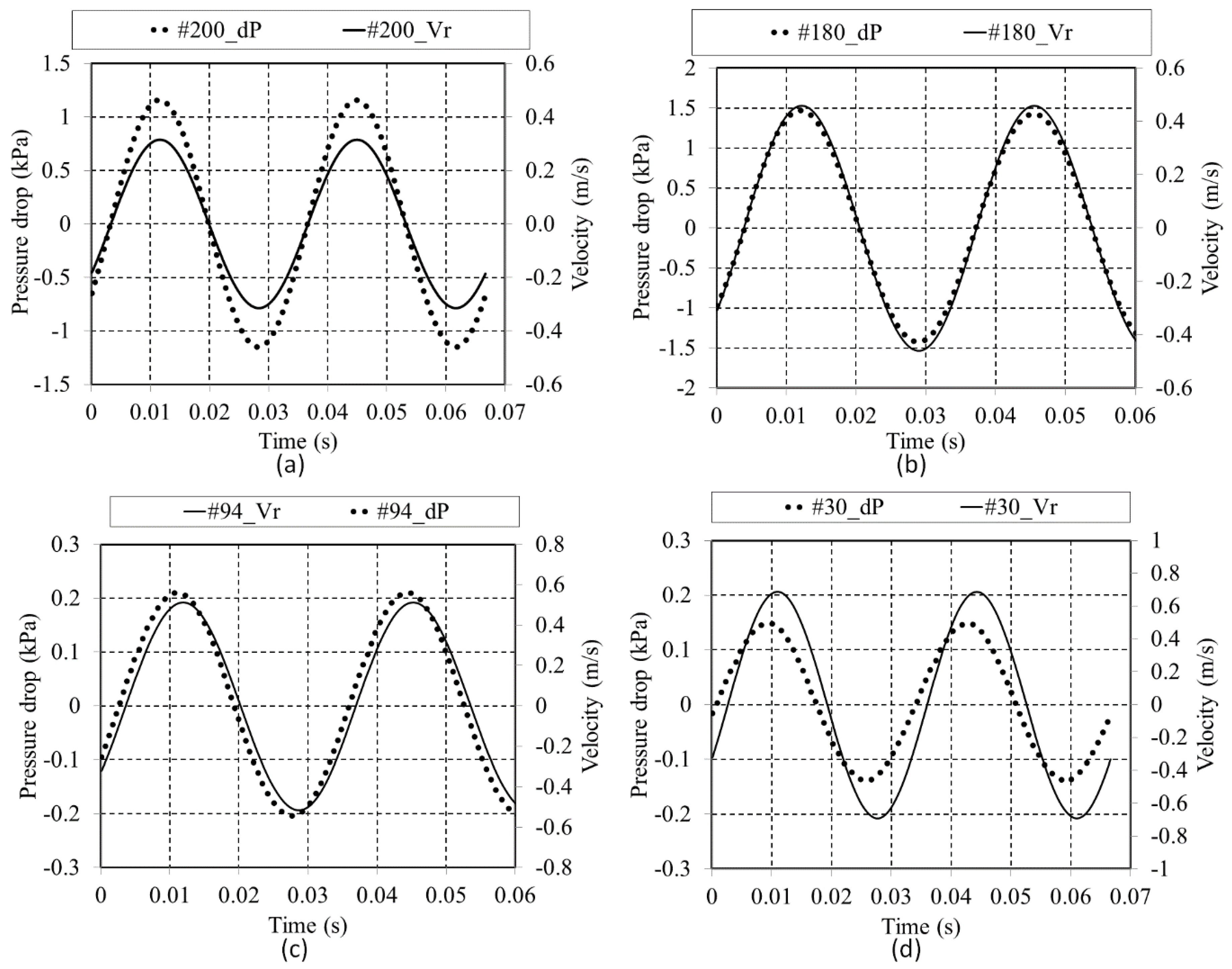
The experimental results are used to calculate the friction factor using Equation (1). The velocity used for calculating the friction correlation of Equation (1) is an averaged value calculated as:

$$u_m=\frac{u_1+u_5}{2\varphi },$$

(17)

where $u_1$ and $u_5$ are the amplitudes of velocities at locations LD and P5, respectively. Strictly speaking, velocity $u_2$ should be included in Equation (17), but this cannot be measured directly. Fortunately, there is only a short distance of empty resonator between locations 1 and 2, while the wave is travelling type. According to early design estimates $u_2\approx u_1$ to within 1%, while $u_1$ is easy to measure directly with the laser displacement sensor. The velocity, $u_m$, represents the actual velocity amplitude in the regenerator. All the regenerator samples are tested at a frequency of 30 Hz and a mean pressure of 25 bar.

3.2. Properties of Gas and Dimensions of Solid Matrix

Four different sizes of mesh screens were tested. The dimensions and parameters of each regenerator mesh screen are listed in

Table 1. Geometric dimensions of regenerators tested.

Mesh Screen Regenerator (Material: Stainless Steel)
Regenerator	Mesh Number	Wire Diameter (mm)	Porosity (%)	Hydraulic Radius (µm)
1	180	0.058	67.5	30.31
2	200	0.041	74.8	30.27
3	30	0.28	72.7	195
4	94	0.089	74.2	63.79

. The working medium is helium, commonly used in thermoacoustic applications because of its good thermal conductivity and specific heat. This allows producing large temperature gradients for a better heat pumping effect. The mesh screen is made of stainless steel. The properties of both the gas and solid material are shown in

Table 2. Properties of helium gas and stainless steel solid matrix.

Properties	Helium	Stainless Steel
Ratio of heat coefficient, $\gamma$	1.6667	-
Speed of sound, $a$ (m/s)	1019.2	-
Density, $\rho$ (kg/m3)	4.0115	7918.1
Specific heat, $c_p$ (J/kg·K)	5193.4	453.84
Gas expansion, $\beta$ (1/K)	3.3333 × 10−3	-
Thermal conductivity, $k$ (W/m·K)	0.15243	14.388
Dynamic viscosity, $\mu$ (kg/m·s)	1.9938×10−5	-

. These properties are obtained at the temperature of 300 K.

4. Computational Model

The regenerator is modelled using a porous medium theory. Two-dimensional Darcy–Forchheimer porous medium equations are expressed as follows [14]:

$$\varphi \frac{\partial \rho }{\partial t}+\nabla ·\left(\rho v\right)=0,$$

(18)

$$\frac{\partial \left(\rho v\right)}{\partial t}+\nabla ·\left(\frac{\rho v·v}{\varphi }\right)+\nabla p-\nabla \left(\mathsf{\tau }\right)=-\left(\frac{\mu \varphi }{K}v+\frac{F{\varphi }^2\rho }{\sqrt{K}}v\left|v\right|\right).$$

(19)

The terms $\varphi$, $\rho$, $t$, $v$, $p$, $\mathsf{\tau }$, $\mu$, $K$ and $F$ represent the porosity, fluid density, time, velocity vector, porous pressure, stress tensor, fluid dynamic viscosity, permeability coefficient and Forchheimer inertial coefficient, respectively. For a homogeneous porous medium with local thermal equilibrium assumption, the one-dimensional energy equation for this porous region is given as [4]:

$$\left[\left(\varphi k_f+\left(1-\varphi \right)k_s\right){\nabla }^{2}T+\left(1-\varphi \right)q_s^{\prime \prime \prime }+v\left(-\frac{\partial P}{\partial x}+{\rho }_{f}g\right)\right]=\left(\varphi {\rho }_f{c}_{pf}+\left(1-\varphi \right){\rho }_s{c}_s\right)\frac{\partial T}{\partial t}+{\rho }_f{c}_{pf}v\frac{\partial T}{\partial x}$$

(20)

where $q_s^{\prime \prime \prime }$ refers to the heat generation rate and $T$ is the temperature. The term $c_p$ is the isobaric specific heat and $c_s$ is the specific heat. The subscripts $f$ and $s$ refer to fluid and solid constituents, respectively. Assuming local thermal equilibrium, the temperature of the gas and solid structure is the same at any time and spatial location due to the condition of perfect thermal contact of the regenerator.

In ANSYS-FLUENT [26], the porous medium is solved using equations given as:

$$\frac{\partial \left(\varphi \rho \right)}{\partial t}+\nabla ·\left(\varphi \rho \mathbf{v}\right)=0,$$

(21)

$$\frac{\partial \left(\varphi \rho \mathbf{v}\right)}{\partial t}+\nabla ·\left(\varphi \rho \mathbf{v}\mathbf{v}\right)+\varphi \nabla \mathrm{p}+\nabla ·\left(\varphi \tau \right)=\varphi B_f-\left(D_x\mu +\frac{C_x\rho }{2}\left|\mathbf{v}\right|\right)v,$$

(22)

$$\frac{\partial }{\partial t}\left(\varphi {\rho }_f{E}_f+\left(1-\varphi \right){\rho }_s{E}_s\right)+\nabla ·\left(v\left({\rho }_f{E}_f+p\right)\right)=\nabla ·\left[k_{eff}\nabla T-\left(\mathsf{\tau }·\mathbf{v}\right)\right].$$

(23)

The term $E_f=c_{p}T-P/\rho +v^2/2$ is the energy of the fluid and $k_{eff}=\varphi k_f+\left(1-\varphi \right)k_s$ is the effective thermal conductivity within the porous regions. Note that the velocity vector v used in ANSYS FLUENT [26] corresponds to the superficial velocity. The real value of velocity within the porous region is obtained by dividing the superficial velocity by the porosity of the region, $\varphi$. Relationships between coefficients $C_x$ and $D_x$ as used in [26] and the coefficients of the standard porous medium theory (permeability coefficient, $K$, and Forchheimer inertial coefficient, $F$) may be obtained by comparing Equations (19) and (22). Note that the viscous dissipation represented by the stress tensor, τ, and the body force, $B_f$, in Equation (22) are neglected. The relationships obtained are shown as follows:

$$K=\frac{{\varphi }^2}{D_x},$$

(24)

$$F=\frac{C_x\sqrt{K}}{2{\varphi }^3}.$$

(25)

These coefficients characterise the hydrodynamic conditions of a porous medium that represent momentum sink (pressure drop) caused by the presence of the medium. As reviewed earlier, the Darcy model suggested that the permeability coefficient alone is enough to represent the pressure drop in a low speed flow. As the speed increases, an inertial effect takes place and the Forchheimer coefficient becomes important to improve the flow model.

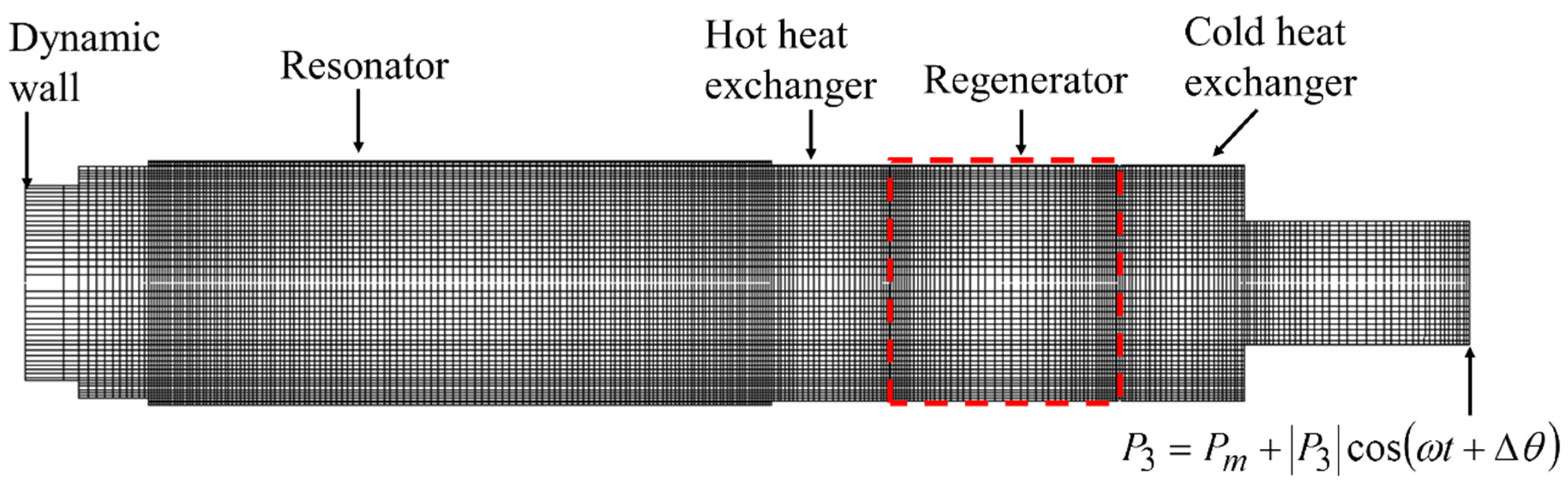
4.1. Computational Domain

Figure 3 presents the two-dimensional axis-symmetrical computational domain used in this study. Flow in the domain occupied by the regenerator is solved using the porous medium theory. Elsewhere, the flow and energy transfer are solved using standard unsteady Navier–Stokes equations available in [26].

A local thermal equilibrium is assumed for the energy equation. Hydrodynamic losses may be attributed to the viscous shear (skin friction) due to the presence of the wall, and a pressure force (form drag) due to the presence of a solid body [8]. Generally, both effects are considered as a package that contributes to resistance losses. However, ANSYS FLUENT [26] defines body forces as separate from the momentum sink that represents the porous medium. Structures investigated in this study have a relatively high porosity. Furthermore, the flow investigated is limited to a low speed. For the conditions of the current study, it is found that the highest pressure drop due to the body force of the porous structure investigated is less than 0.1%, and hence is neglected.

In this study, the porous medium has been treated as isotropic. The losses in the direction other than the main flow direction were assumed small and negligible. The inertial effect was neglected because of the low speed of the flow. Pressure and velocity were expressed in terms of mean components and first order fluctuating components (except that the mean velocity is zero). The simple harmonic equations (cf. Figure 3) were applied in defining the boundary conditions of the computational domain.

A dynamic mesh was imposed as the inlet boundary condition to replicate the movement of the piston of the linear motor. The dynamic mesh area and the resonator are separated by a short tube (15 mm in length and 50 mm in diameter). The computational domain excluded the RLC network, but imposed the phase control using a user-defined-function (UDF) at the inlet wall and the exit pressure at location P3 (refer to Figure 2 and Figure 3). The last region after the cold heat exchanger is 75.5 mm long and has a diameter of 27.17 mm. The working gas was treated as a compressible ideal gas. The model has been solved using an unsteady pressure-based implicit solver with the first order implicit scheme for the discretisation of time. For model that uses dynamic mesh, the time discretisation scheme is only available in ANSYS as first order calculation [26]. Therefore, first order calculation with implicit scheme was used. The time step size was set to 1.11111 × 10⁻⁴ s (which corresponds to 300 steps per acoustic cycle at frequency of 30 Hz) so that convergence could be achieved within 15–18 iterations per time step. The convergence was set to 10⁻⁴ for continuity and momentum equations and 10⁻⁶ for energy equation. Pressure–velocity coupling has been solved using pressure-implicit-with-splitting-operators (PISO) algorithm available in ANSYS FLUENT [26]. All variables (pressure, density, momentum and energy) were discretised using second-order upwind method. The model was run until steady oscillatory flow condition was achieved. The steady oscillatory condition was monitored through the time history data of velocity inside the resonator. It was observed that the model needs to be run for at least five cycles in order to achieve the steady oscillatory flow condition.

The operating pressure was set at 25 bar. The flow has a frequency of 30 Hz. Temperatures at the location of the hot and cold heat exchangers were set as constants with values following the measured temperatures in the experiment. The temperature developed reflects the result of the thermoacoustic effect occurring at the regenerator when the travelling-wave time phasing is set. The temperature gradient within the regenerator, for all mesh screen samples, varies depending on the acoustic excitation and type of mesh screens used. In an attempt to minimize the effect of temperature on the pressure readings, the development of temperature gradient has been controlled using cold heat exchanger. For all regenerator samples tested here, the recorded temperature gradient varies in a range of $10 °C\le \Delta T\le 21 °C$. The values of temperature from experiments are used in the model so that the effect of the small temperature variations on pressure readings are being modelled following the experimental findings.

The contribution of pressure loss from the heat exchanger has been calculated using the pressure drop prediction for a compact heat exchanger as presented in [8]:

$$\frac{\Delta p}{p_1}=\frac{v_1^2/2g}{p_1/{\rho }_1}\left[\left(K_c+1-{\varphi }^2\right)+2\left(\frac{1}{\rho }-1\right)+f\frac{L}{r_h}\rho -\frac{1}{\rho }\left(1-{\varphi }^2-K_e\right)\right].$$

(26)

The subscript 1 refers to parameters obtained at the inlet of the heat exchanger. The terms $p$, $v$, $\rho$, $g$, $\varphi$, and $r_h$ refer to pressure, velocity, fluid density, gravity, porosity and hydraulic radius, respectively. Parameters $K_c$, $K_e$ and $f$ are the entrance losses, exit losses and Fanning friction losses, respectively, as given in [8]. The calculations showed that the contribution of cold heat exchanger losses was within 1%–5% of the whole pressure drop measured between locations P2 and P5. The loss varies according to the range of velocity and pressure drop achieved in the experiment. The overall contribution of losses is small because of the low speed of flow. The calculated loss was deducted from the total pressure measured in the experiment. The hydrodynamic condition of the regenerator for CFD modelling was gained by determining the permeability coefficient that gives a pressure drop similar to the experimentally measured value.

4.2. Pressure Drop and Grid Size

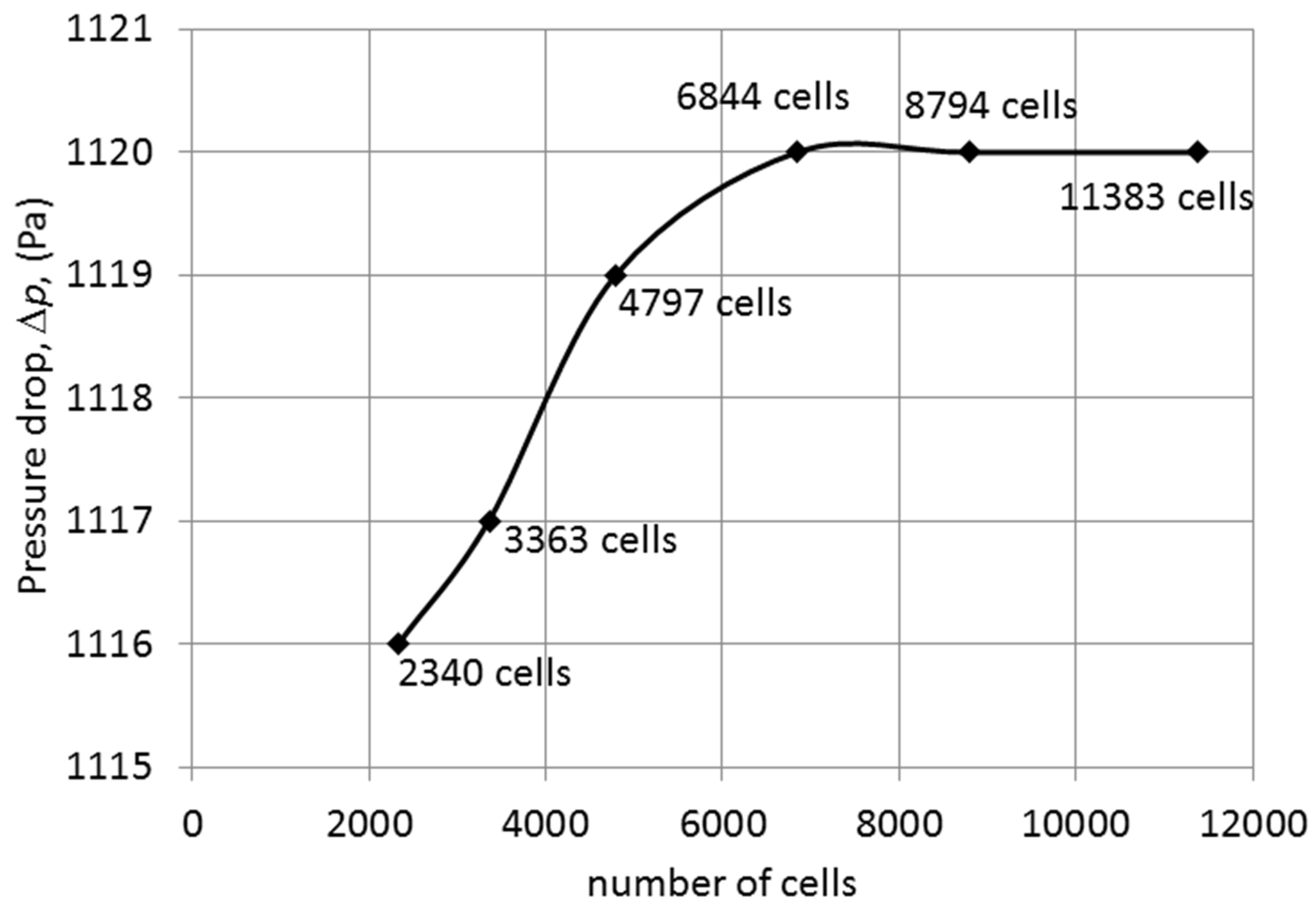
The mesh was defined to be denser near the wall and at the interfaces between the rig components inside the resonator. The mesh near the dynamic wall was made coarser to allow for the movement of the wall. The grid independency test has been carried out by increasing the number of mesh points by a factor of 1.3. The grid structure remained unchanged with only the mesh density being increased. The resulting pressure drop obtained for grids of different sizes is shown in Figure 4. A grid size with a total number of cells of 8794 has been found to be sufficient to provide a solution that is independent of the grid and therefore selected for this investigation. The model has also been run in both single and double precision solver in readiness to test for round-off error. It appears that the single precision is sufficient to solve this two-dimensional axis-symmetrical model.

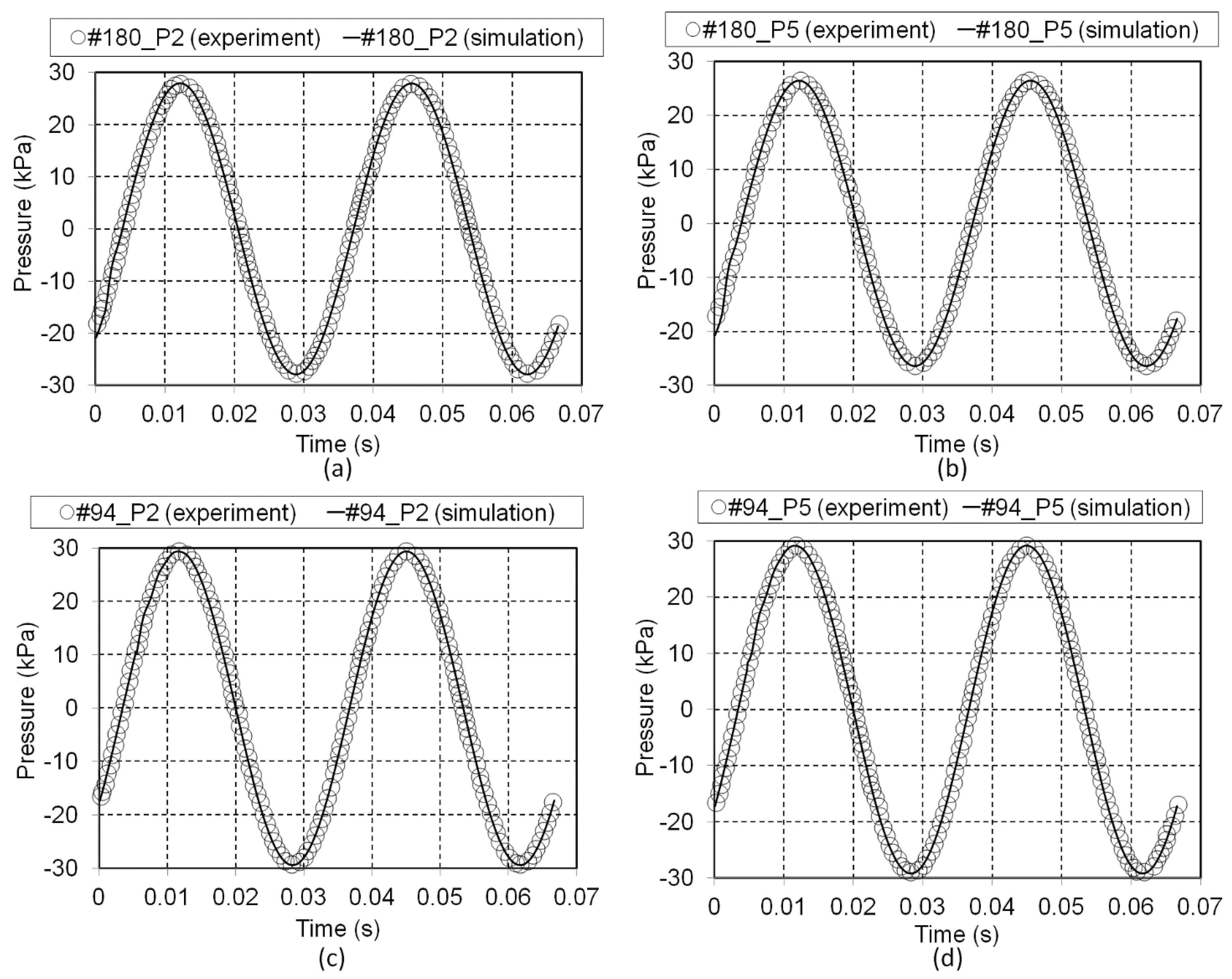
4.3. CFD Model Validation

The model was pre-validated for boundary conditions and subsequently the porous coefficients $C_x$ and $D_x$ were set followed by the final validation of the porous model. In the pre-validation stage, only the velocity and pressure at the location before the porous medium (locations P1 and P2 in Figure 2) were compared to the experiment. A good agreement was found as shown in Figure 5.

Once the model had been pre-validated, the permeability coefficient, K, of the regenerator was then predicted by carefully increasing the permeability value in ANSYS FLUENT [26] until the pressure drop matched the experimental value. As soon as the pressure drop matched, the validation was finalised by comparing the inlet velocity, calculated from the measured displacement of linear motor’s piston (V1 in Figure 5), and pressures at locations P2 and P5 (definition of locations is given in Figure 2). The same procedure was repeated for each case until a good agreement with the experiment was obtained for all samples tested. Figure 6 shows the results for pressure at locations P2 and P5 after the permeability tensor set matched the pressure drop measured in the experiment.

5. Results and Discussion

The hydrodynamic conditions of the regenerator samples tested are presented as friction factor. The friction factor was derived from the Darcy model and results are presented using the permeability coefficients obtained from the numerical work. Comparison to experimental results and Swift and Ward correlation [7] is also made. Further analysis on the phase angle between pressure and velocity is also shown.

5.1. Friction Factor Correlation

In the porous medium theory, the friction factor of most porous media is presented by the permeability Reynolds number, $R{e}_K= \rho u{K}^{1/2}/\mu$. The pressure drop characteristics of the porous medium are related to the permeability Reynolds number as given by [4]:

$$-\nabla P=\frac{1}{2}\frac{f\rho u^2}{\sqrt{K}}.$$

(27)

The pressure gradient can also be represented by the Darcy–Forchheimer model as in Equation (7). The following formula can be derived from Equations (7) and (27):

$$f=\frac{2\sqrt{K}}{\rho u^2}\left[\frac{\mu }{K}u+\frac{F\rho }{\sqrt{K}}{u}^2\right].$$

(28)

Further modification of Equation (28) can be made to include the hydraulic diameter as follows:

$$f=\frac{2\sqrt{K}}{\rho u^2}·\frac{d_h}{d_h}\left[\frac{A_1\mu }{K}u+\frac{A_{2}F\rho }{\sqrt{K}}{u}^2\right],$$

(29)

$$f=\frac{2d_h}{\sqrt{K}}·\frac{A_1}{R{e}_h}+2A_{2}F.$$

(30)

The permeability coefficient, $K$ has a unit (length)² and the Forchheimer inertial coefficient, $F$, is dimensionless. Parameters $A_1$ and $A_2$ are constants introduced to correlate the equation to fit the experimental result. Simple dimensional analysis shows that Equation (30) is dimensionless. The derived correlation agrees with the well-known Ergun form presented in Equation (3). From this derived friction factor, the coefficients $a_1$ and $a_2$ in the Ergun equation are defined as:

$$a_1=\frac{2A_1{d}_h}{\sqrt{K}},$$

(31)

$$a_2=2A_{2}F.$$

(32)

In the simplest Darcy model, when the velocity is small, the inertia effect is neglected and the friction factor is left with only first term of right-hand side of Equation (30):

$$f=\frac{2d_h}{\sqrt{K}}·\frac{A_1}{R{e}_d}.$$

(33)

Finally, with this correlation the porous coefficient predicted through CFD model is used to predict the friction factor of the porous medium and then compared to the experimentally calculated friction factor for the actual sample. The friction factor correlation presented in Equation (33) is derived from the Darcy correlation. Hence comparing the simulation results to experiment requires the friction factor predicted by simulation model to be divided by four. In this study, all comparisons are carried out in line with the Fanning-based correlation. The Fanning-based correlation for computational models is given as:

$$f=\frac{d_h}{2\sqrt{K}}·\frac{A_1}{R{e}_d}.$$

(34)

Permeability is an empirical constant used in the porous medium community to characterize the ability to transmit fluid by the porous media. The permeability coefficients for the regenerator samples investigated, obtained from the CFD-assisted method, are tabulated in

Table 3. CFD-predicted permeability for regenerator investigated.

Regenerator Mesh Screen Numbers	#200	#180	#94	#30
Permeability, $K$ (m2)	1.1505 × 10−10	0.99012 × 10−10	10.5715 × 10−10	41.29 × 10−10

.

A higher regenerator mesh number refers to a finer mesh. This is reflected by the value of the wire diameter of each sample as listed in Table 1. The permeability is high for a regenerator with a mesh screen number of #30 and decreases as the regenerator mesh screen number increases to #200 (the value for #180 being slightly outside this trend due to a lower porosity value—cf. Table 1). The permeability coefficient in Table 3 is used to calculate the friction factor using Equation (34). Several cases of measurement and numerical prediction were considered for each sample. These corresponded to different level of acoustic excitation produced by the linear motor, and result in different values of Reynolds number, $R{e}_d$, as defined in Equation (6). The results are plotted in Figure 7.

In Figure 7, there are 17 square, nine triangle, six circle and 11 diamond symbols that represent tests of samples #180, #200, #94 and #30, respectively. A fit can be obtained for all the cases as shown by the line in the figure. The friction data obtained from the numerical model fitted the following correlation:

$$f=\frac{d_h}{2\sqrt{K}}·\frac{1.48}{R{e}_d}.$$

(35)

The correlation was obtained based on the least-square fit with a confidence level of 95%. The correlation represents a friction loss of all the four regenerator mesh screens tested. The correlation best represents the hydrodynamic losses of high regenerator mesh numbers and slightly under-predicts the losses occurring at a regenerator build with low mesh screen numbers. The maximum difference between the correlation and the friction value of regenerator with low mesh screen number are 30% and 50% for #94 and #30, respectively. The diamond symbols for $R{e}_d$ larger than 60 are clearly deviating from the line. This may be due to the fact that for large Reynolds number and a very coarse size of regenerator mesh screens the Forchheimer inertial coefficient may become significant and Equation (30) may apply. The constant 2 in the denominator of Equation (35) is the result of the conversion from Darcy-based correlation to Fanning-based correlation and left on purpose for clarity.

Figure 8 shows that the numerical results represented by correlation (35) and the results calculated using Swift and Ward [7] correlation (cf. Equations (3)–(5)) both qualitatively agree with experimental measurement. Swift and Ward [7] defined their friction correlation using Darcy-based correlation, and therefore the results calculated through Equation (3) through to Equation (5) need to be divided by 4 for comparison. The results indicate that the assumption used by Swift and Ward [7] is acceptable. The assumption states that pressure drop and velocity relate in a similar way as in steady flows [7]. There are arguments found in the literature that claimed that a pressure drop condition in oscillatory flow deviated from predictions of steady flow. An explanation to that situation could relate to the influence of phase-shifting between pressure and velocity. Further discussion of this is provided in Section 5.2 for low mesh number regenerators. Current results have shown that a pressure drop condition for an oscillatory flow with travelling-wave time-phasing does not deviate much from the Swift and Ward’s correlation, especially when the mesh number is high.

5.2. Analysis of Phase Shift

Phase angle between pressure and velocity oscillations is important in determining the hydrodynamic condition of porous media such as the regenerators. If the pressure and velocity are not in phase, the maximum pressure occurs at a certain phase lag compared to maximum velocity. Then, the amplitude data may not be accurate enough to represent the friction factor according to Equation (1).

In other studies [10,11,18], the phase shift between pressures at location before and after the regenerator is observed when the operating frequency increases. The phase shift effect is observed even at a frequency as low as 5 Hz in the results presented by Cha et al. [18]. Zhao and Cheng [17] reported that the phase shift between pressure and velocity in the experimental investigation appeared at a very low kinetic Reynolds number (calculated to be equivalent to 2.5 Hz).

In the current experiment, it is not possible to measure the pressure drop and velocity amplitude within the regenerator. However, the numerical model is validated for several points within the rig. Thus, it is reasonable to expect that it will reliably predict the pressure drop and velocity within the regenerator.

Figure 9 shows the pressure drop and velocity within the regenerator. The pressure drop was calculated using values obtained at locations P2 and P5, where pressure sensors are available. Note that vertical scales of the plots in Figure 9 vary. This was done deliberately to show more clearly the changes in phase difference between pressure and velocity. For fine regenerator mesh screens (#200 and #180), the pressure drop is in phase with the velocity within the regenerator. When the mesh screen is coarser (#30 and #94), the pressure drop becomes slightly out of phase from the velocity within the regenerator. The pressure drop tends to lead the velocity more visibly as the mesh becomes coarser. Theoretically, bigger porosity results in a lower flow velocity within the porous region, if set at a similar level of acoustic excitation. The shear stress and form drag is likely to be smaller too. However, due to the limitation of the experimental setup, data for coarse mesh number are only available for a relatively high Reynolds number. Similarly, data for fine mesh are only available for the low Reynolds number region. Therefore, it is possible that the phase shift between pressure and velocity seen within the coarse mesh is due to the relatively high velocity excited by the linear motor. This could be the reason for the time delay between pressure drop and velocity. It is likely that the phase shift between pressure and velocity is the feature of the inertial effect described by the Forchheimer model.

6. Conclusions

Modelling the full state of a regenerator may be very computationally demanding due to the very small size of pore and the tortuosity of the structure. Hence, in this study, an economical way of modelling a regenerator is developed. A two-dimensional model has been developed for the regenerator working in a travelling-wave setting. The structure is modelled as a porous medium. Modelling a porous medium requires a proper closure model to represent the momentum losses and thermal inertia of the flow due to the presence of the structure. In this study, the momentum losses are modelled with pressure drop data gained from the experiment conducted in a well-controlled travelling-wave condition.

The pressure drop of the porous tortuous structure of the regenerator has been modelled and validated by the results obtained from experiment carried out in an apparatus where a control could be achieved over the phase angle between velocity and pressure thus enabling a travelling-wave condition to be imposed. The values of computationally determined permeability coefficient, K, that represents the hydrodynamic loss of the regenerator investigated, are shown in Table 3. Friction factor correlation has been developed based on a porous medium model. A simplification offered by Darcy’s law has been used for the low speed condition studied. 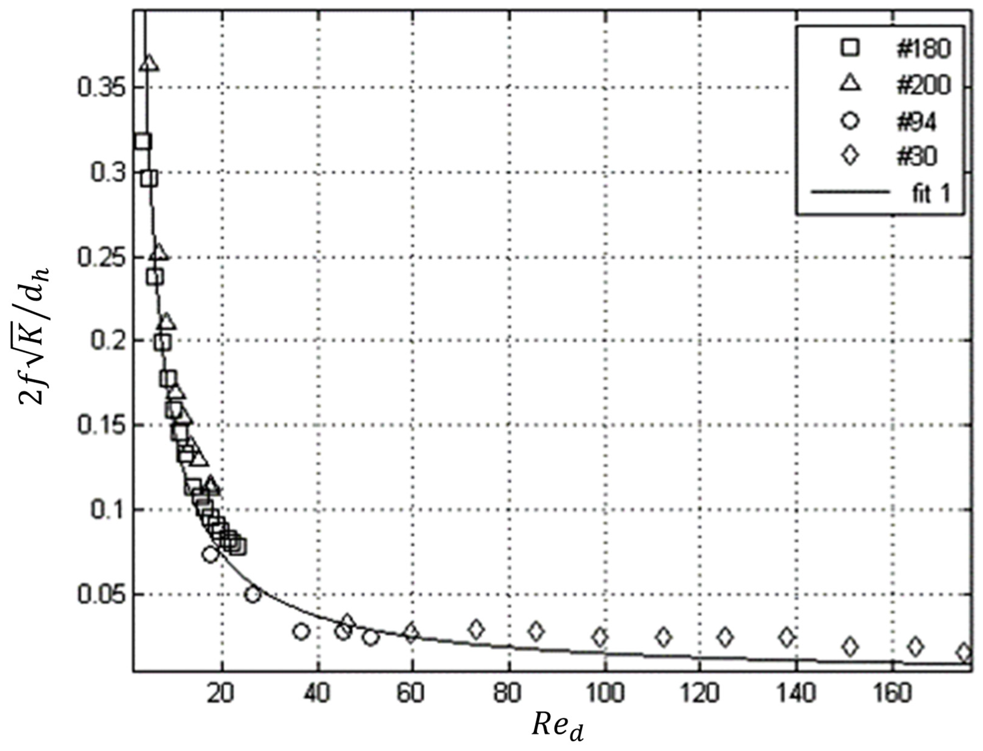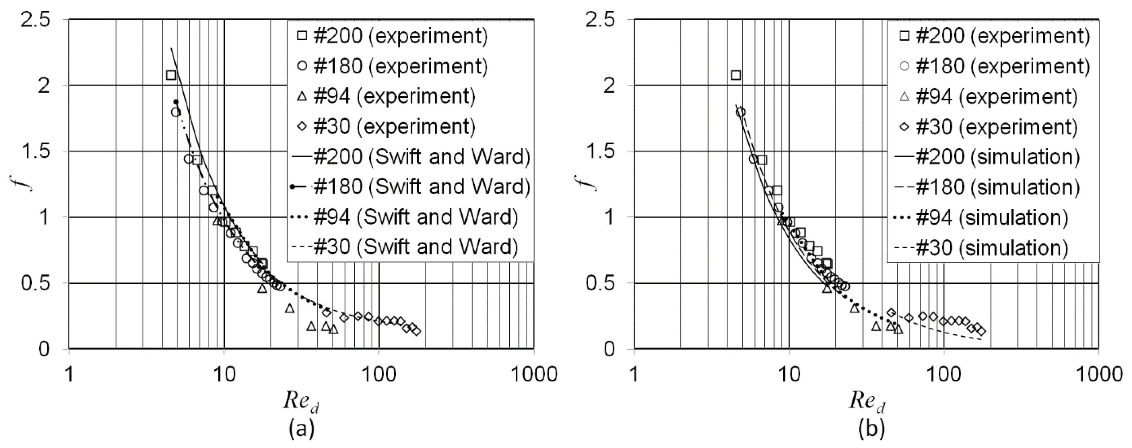The results from this correlation appear to match the results calculated through the correlation proposed by Swift and Ward [7]. This indicates that steady flow assumptions, used by them when developing their correlation, apply to the travelling-wave conditions investigated here.

This study suggests that the difference in friction correlation between oscillatory flow and steady flow, as reported in many previous studies, may be related to the “phase shifting” between pressure and velocity which are used for predicting the friction factor. For a travelling-wave system, when the pressure and velocity are in-phase, the pressure drop and velocity relate to each other in a similar way as in a steady flow. Results of this investigation show that the pore size of the mesh screen used in a travelling-wave system should not be too large. Otherwise, difficulties in sustaining the travelling-wave phase angle within the regenerator may arise. Should this happen the friction correlation may need to be revised to account for the effect of the “phase shifting” phenomenon.

Unfortunately, the results obtained from the experiment are somewhat limited because of the design of the apparatus. Flow within samples made of fine mesh screen was limited to low Reynolds number, while the flow within samples made of coarse mesh screen was at a relatively high Reynolds number (otherwise a sufficient pressure drop could not be recorded). Phase shift was observed between pressure and velocity within the regenerator made of coarse mesh screen (#94 and #30). The phase shifting phenomenon may be related to the inertial effect described by the Forchheimer model. This may be the reason for the discrepancy between numerical and experimental results at Reynolds number higher than 60.

The central focus of this study is pressure drop. However, thermal condition of the regenerator is also an important criterion to consider when selecting a regenerator. This can be done for example on the basis of Equation (24) in reference [3], while similar insights are also available in references [7,24]. A regenerator with a coarse mesh screen may be favourable in that it provides a smaller pressure drop. Nevertheless, the thermal contact may not be as good as for the fine mesh. Further investigation on this subject is strongly suggested to cover the whole range of the thermoacoustic phenomena, including the heat transfer within the regenerator.