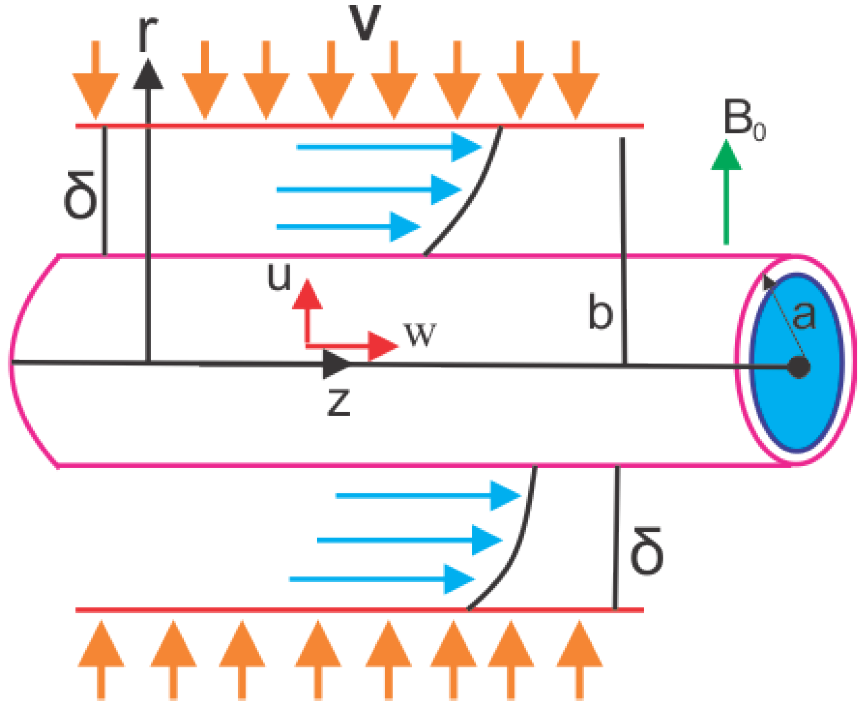
Figure 1.
Geometry of the Physical Model.
Figure 1.
Geometry of the Physical Model.
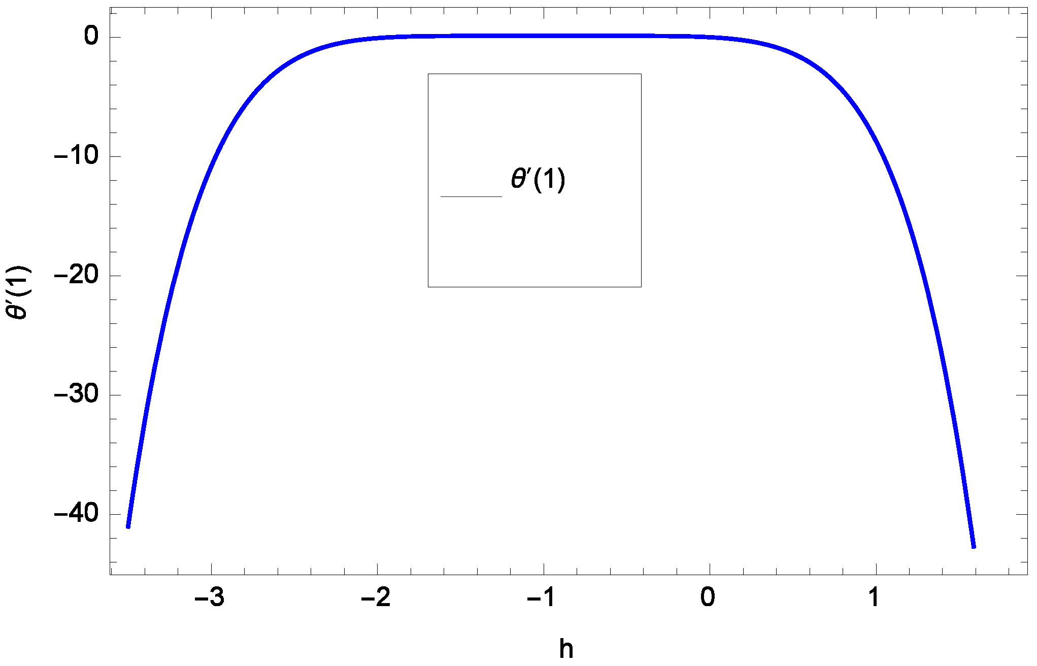
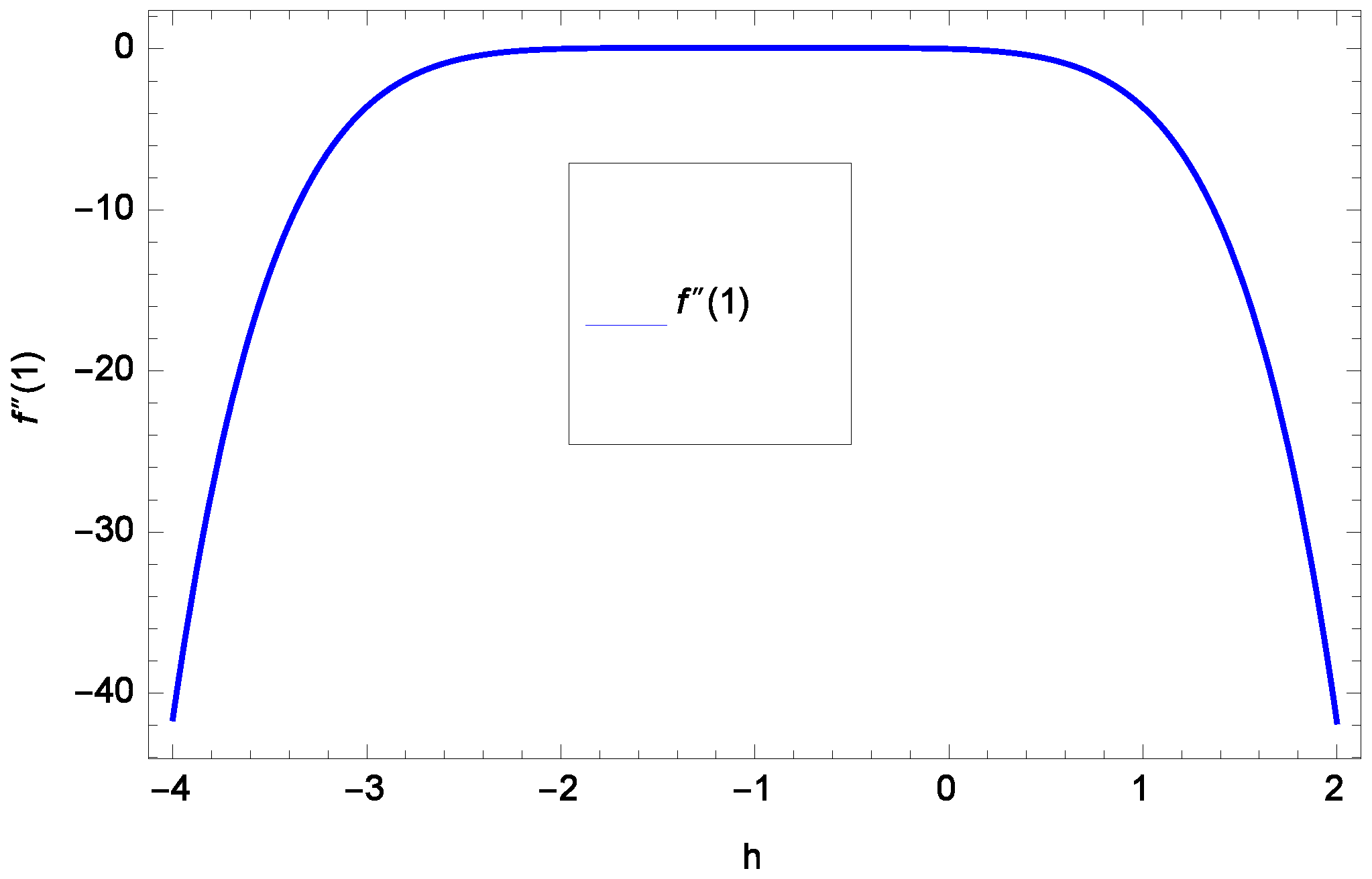
Figure 2.
h curve of f(ζ).
Figure 2.
h curve of f(ζ).
Figure 3.
h curve of .
Figure 3.
h curve of .
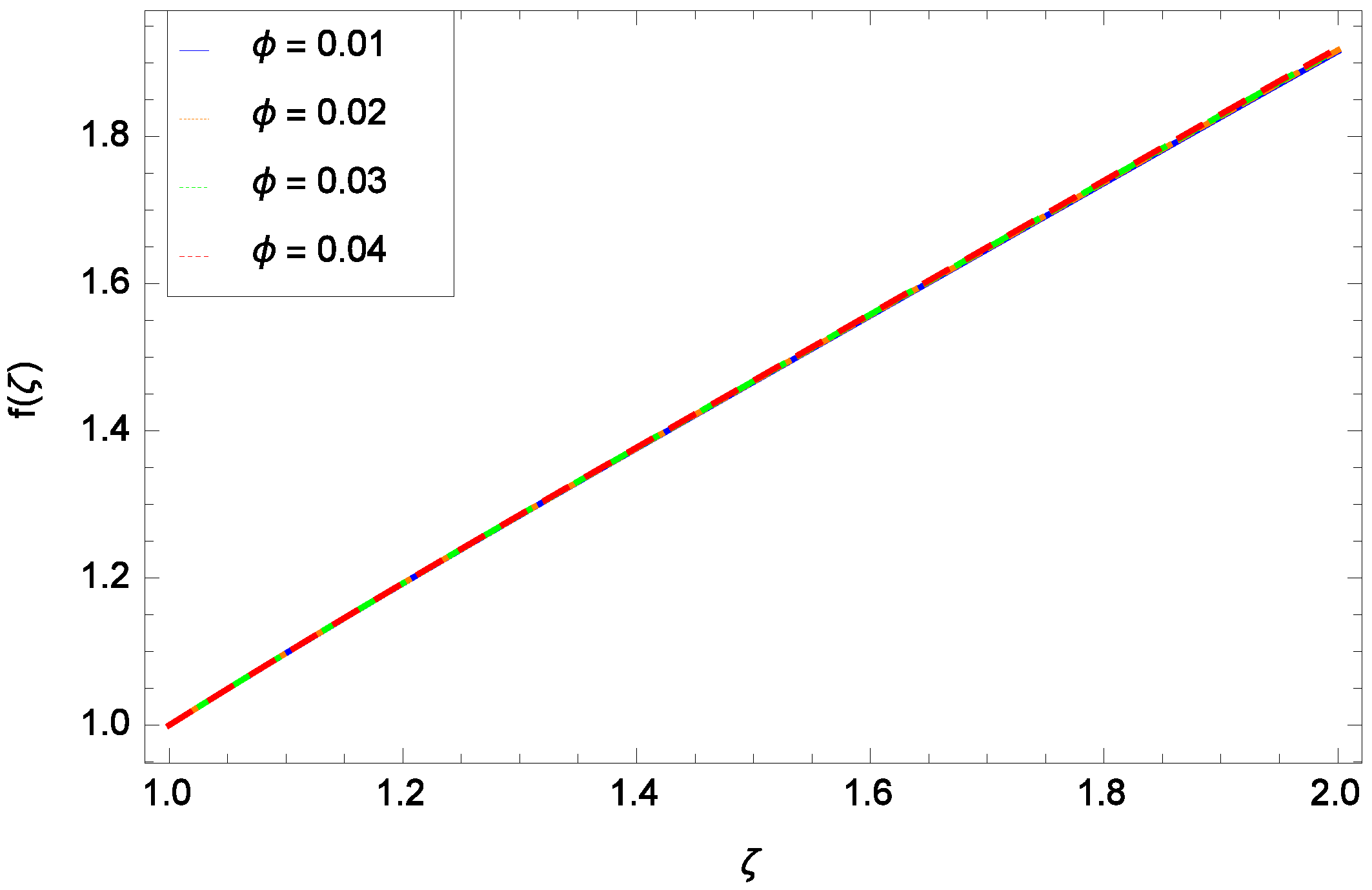
Figure 4.
Non-dimensional velocity f(ζ) sketch for h = − 0.10, M = 0.10, Re = 0.70, = 0.04, Pr = 6.80 and various values of (CuO-HO).
Figure 4.
Non-dimensional velocity f(ζ) sketch for h = − 0.10, M = 0.10, Re = 0.70, = 0.04, Pr = 6.80 and various values of (CuO-HO).
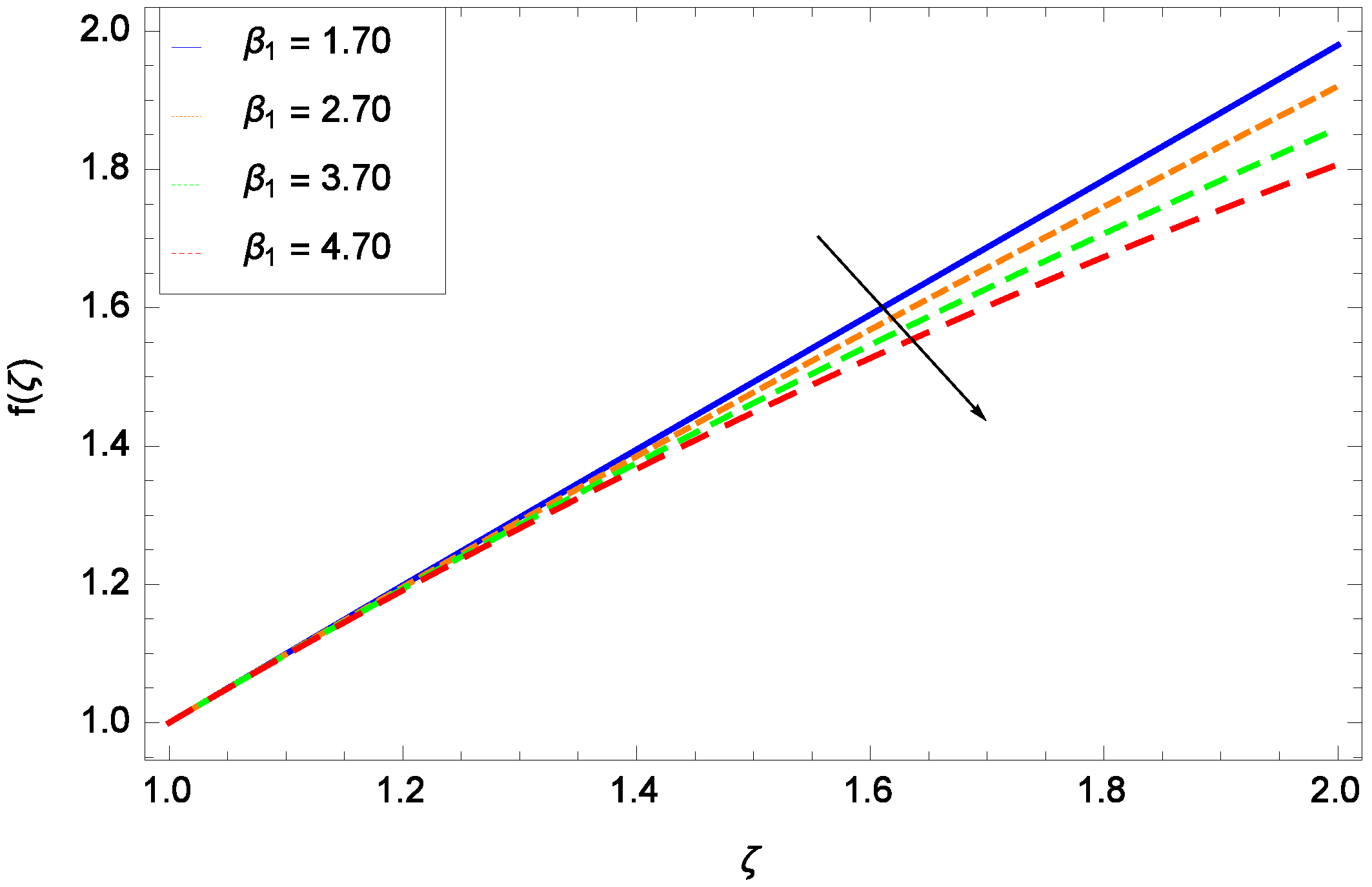
Figure 5.
Non-dimensional velocity f(ζ) sketch for h = −1.10, = 1.70, M = 0.10, Re = 0.70, Pr = 6.80 and various values of (CuO-HO).
Figure 5.
Non-dimensional velocity f(ζ) sketch for h = −1.10, = 1.70, M = 0.10, Re = 0.70, Pr = 6.80 and various values of (CuO-HO).
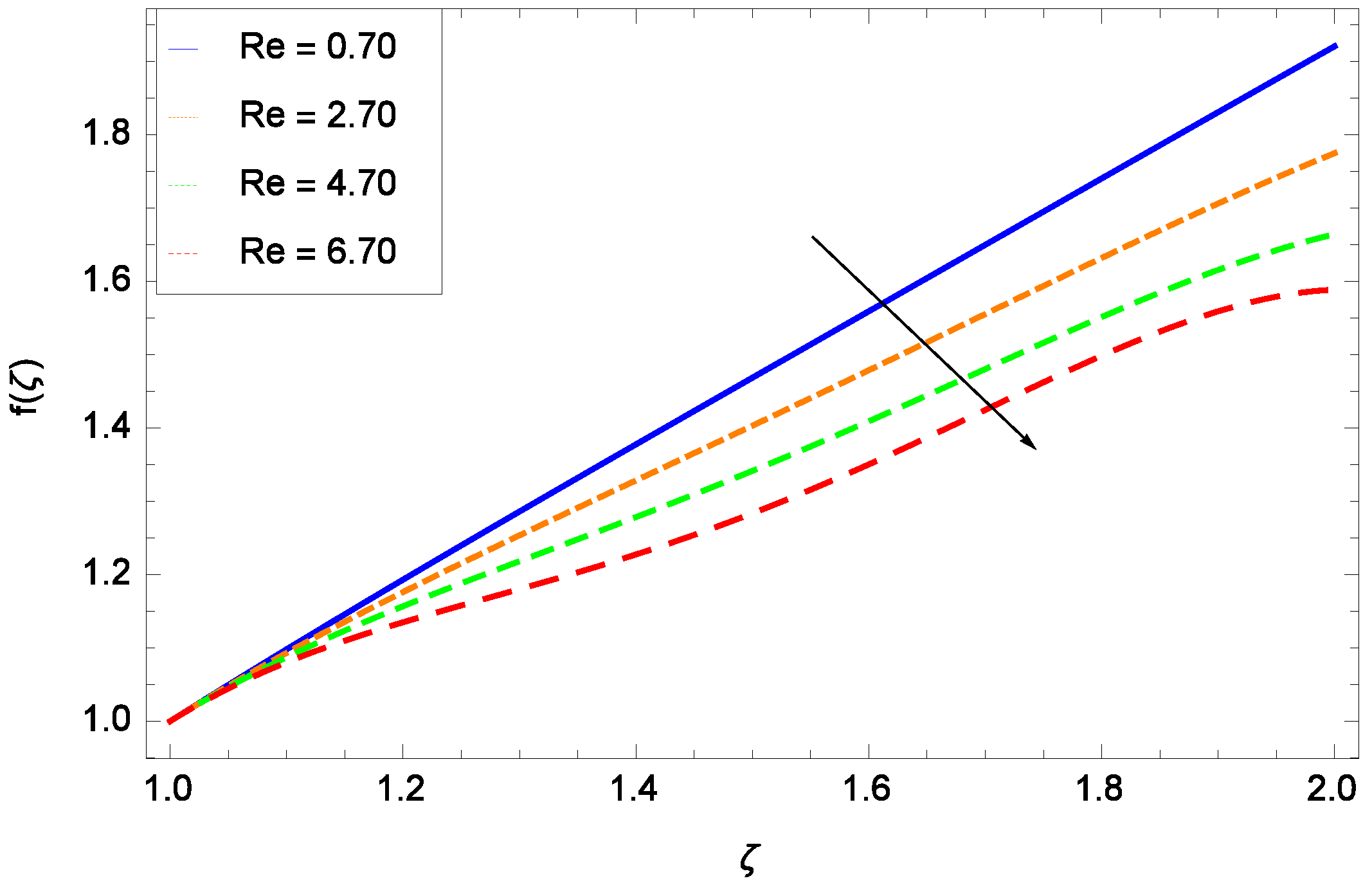
Figure 6.
Non-dimensional velocity f(ζ) sketch for h = −1.10, = 1.70, M = 0.10, = 0.04, Pr = 6.80 and greater quantities of Re (CuO-HO).
Figure 6.
Non-dimensional velocity f(ζ) sketch for h = −1.10, = 1.70, M = 0.10, = 0.04, Pr = 6.80 and greater quantities of Re (CuO-HO).
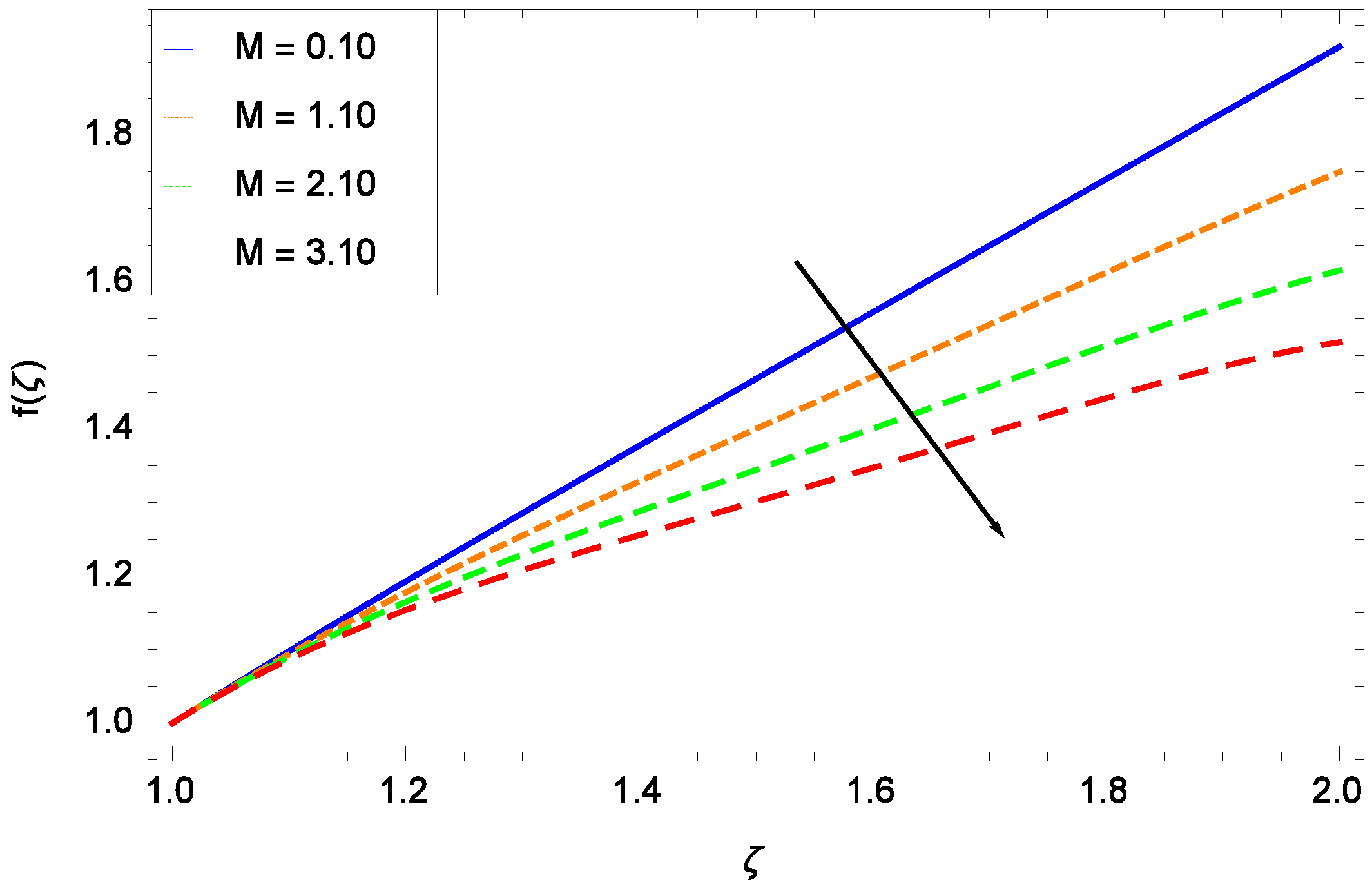
Figure 7.
Non-dimensional velocity f(ζ) sketch for h = −1.10, = 1.70, M = 0.10, Re = 0.70, = 0.04, Pr = 6.80 and greater quantities of M (CuO-HO).
Figure 7.
Non-dimensional velocity f(ζ) sketch for h = −1.10, = 1.70, M = 0.10, Re = 0.70, = 0.04, Pr = 6.80 and greater quantities of M (CuO-HO).
Figure 8.
Non-dimensional temperature θ(ζ) sketch for h = −0.10, M = 2.00, Re = 5.00, = 0.04, Pr = 6.80 and various values of (CuO-HO).
Figure 8.
Non-dimensional temperature θ(ζ) sketch for h = −0.10, M = 2.00, Re = 5.00, = 0.04, Pr = 6.80 and various values of (CuO-HO).
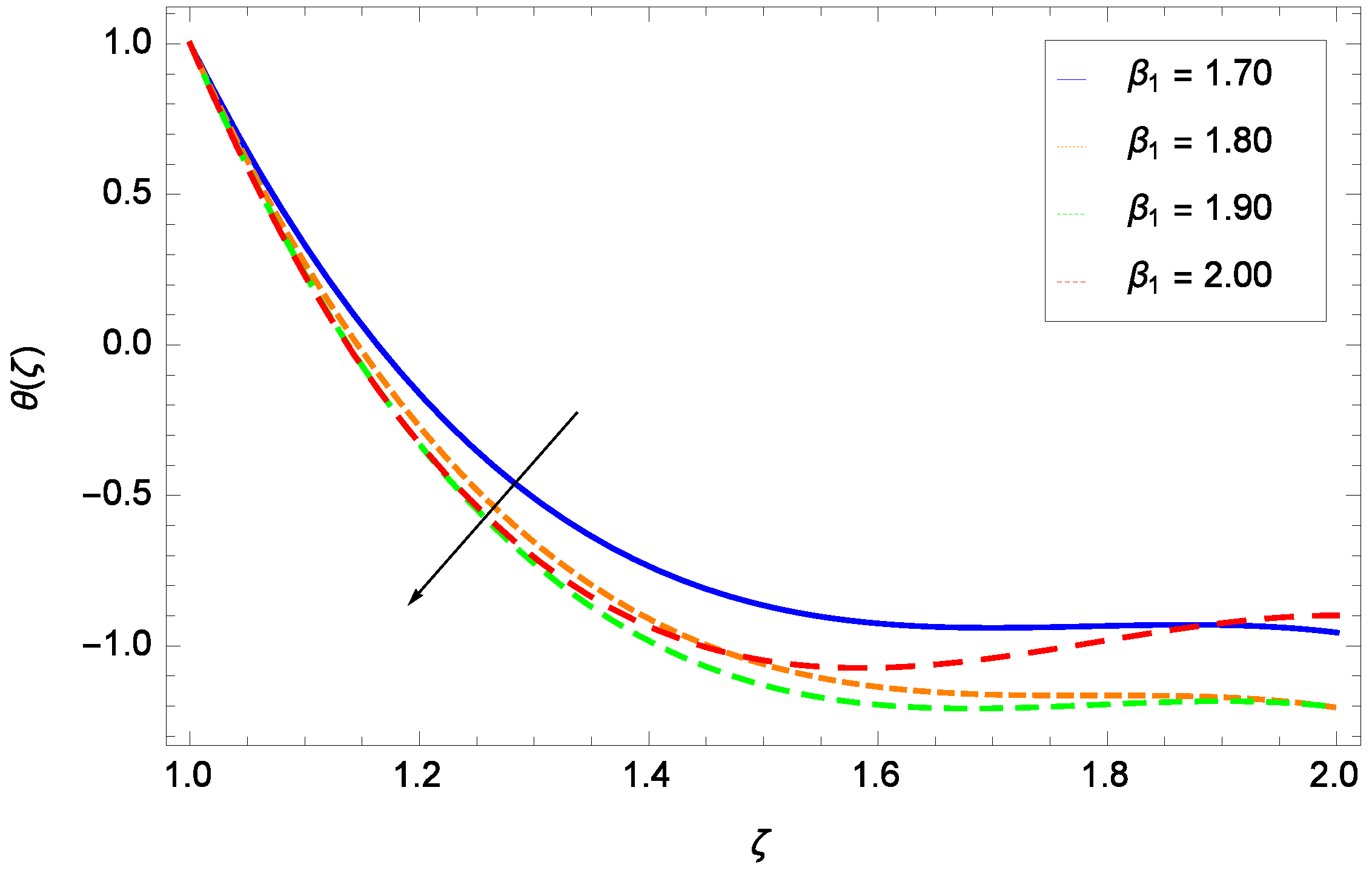
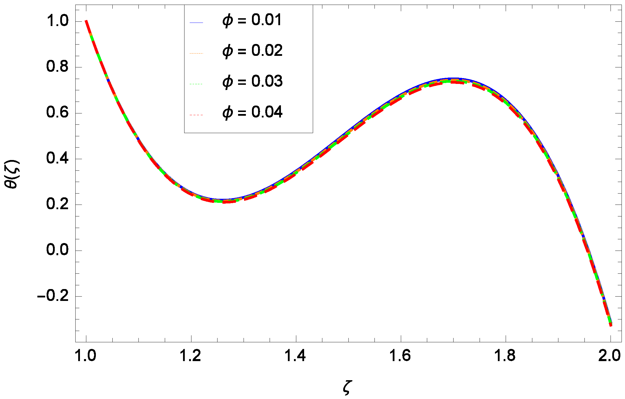
Figure 9.
Non-dimensional temperature θ(ζ) sketch for h = −1.10, = 1.70, M = 0.10, Re = 0.70, Pr = 6.80 and various values of (CuO-HO).
Figure 9.
Non-dimensional temperature θ(ζ) sketch for h = −1.10, = 1.70, M = 0.10, Re = 0.70, Pr = 6.80 and various values of (CuO-HO).
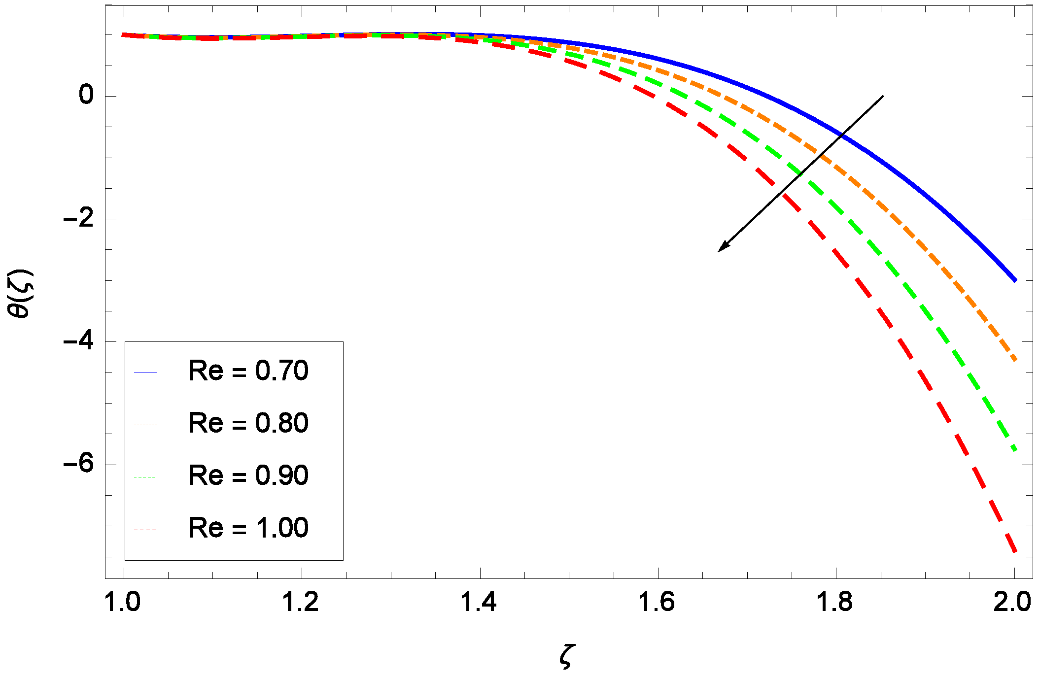
Figure 10.
Non-dimensional temperature θ(ζ) sketch for h = −1.10, = 1.10, = 0.04, M = 0.10, Pr = 6.80 and greater quantities of Re (CuO-HO).
Figure 10.
Non-dimensional temperature θ(ζ) sketch for h = −1.10, = 1.10, = 0.04, M = 0.10, Pr = 6.80 and greater quantities of Re (CuO-HO).
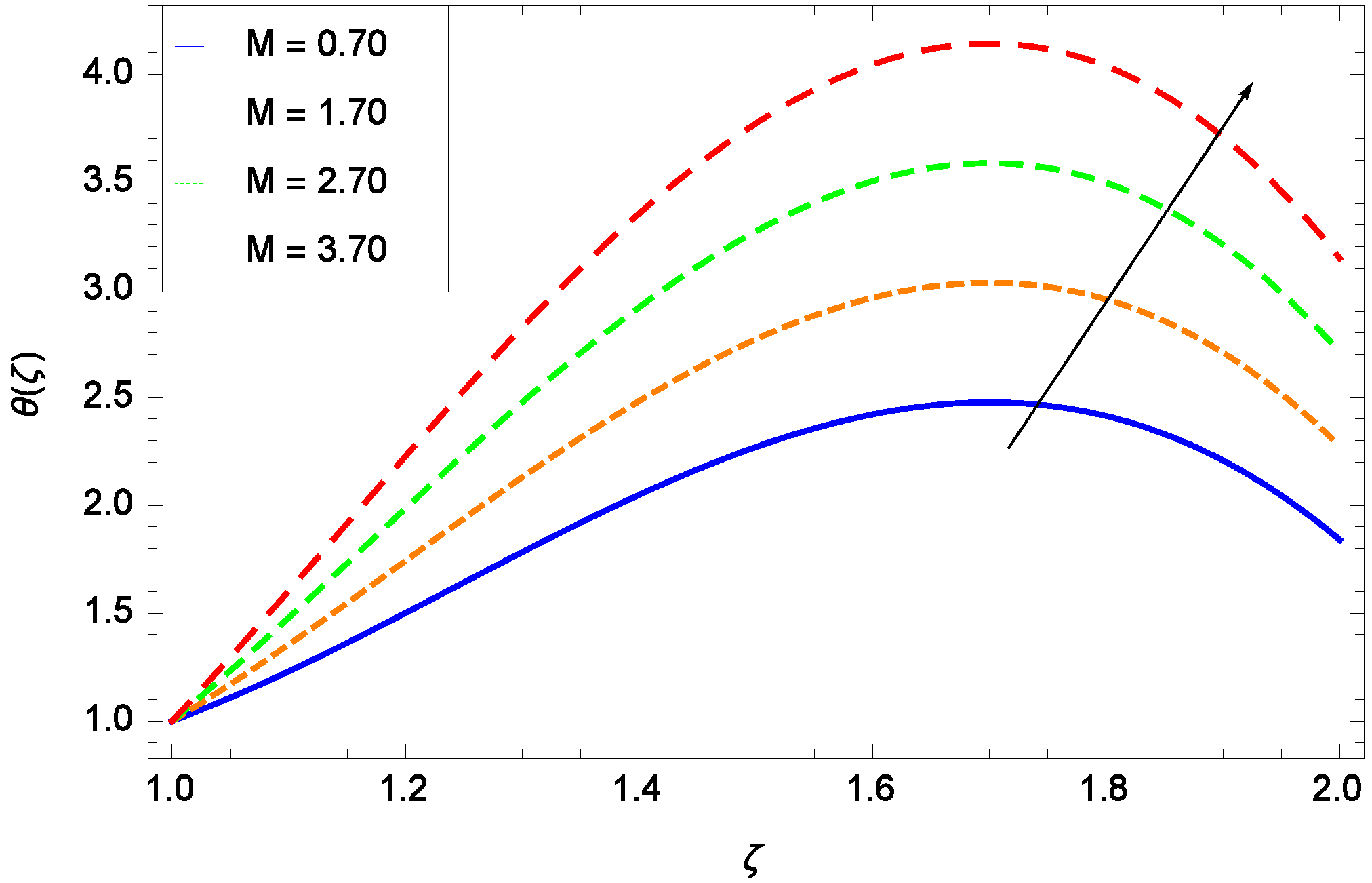
Figure 11.
Non-dimensional temperature θ(ζ) sketch for h = −2.50, = 1.70, = 0.04, M = 0.10, Pr = 6.80 and greater quantities of M (CuO-HO).
Figure 11.
Non-dimensional temperature θ(ζ) sketch for h = −2.50, = 1.70, = 0.04, M = 0.10, Pr = 6.80 and greater quantities of M (CuO-HO).
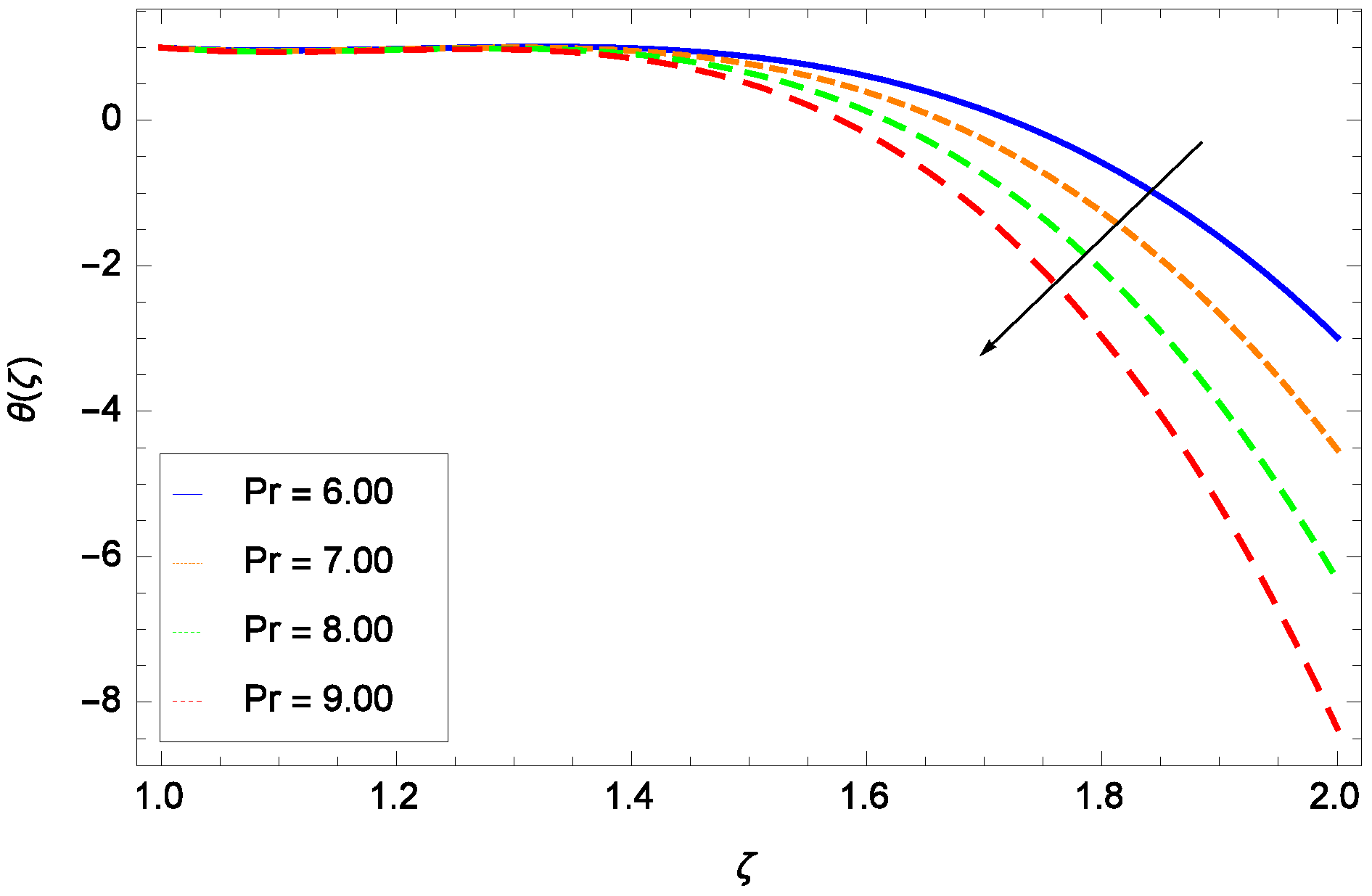
Figure 12.
Non-dimensional temperature θ(ζ) sketch for h = −1.10, = 1.10, M = 0.10, = 0.04, Re = 0.70 and various values of Pr (CuO-HO).
Figure 12.
Non-dimensional temperature θ(ζ) sketch for h = −1.10, = 1.10, M = 0.10, = 0.04, Re = 0.70 and various values of Pr (CuO-HO).
Figure 13.
Non-dimensional Pressure (ζ) sketch for h = −0.10, M = 0.10, Re = 0.70, = 0.04, Pr = 6.80 and various values of (CuO-HO).
Figure 13.
Non-dimensional Pressure (ζ) sketch for h = −0.10, M = 0.10, Re = 0.70, = 0.04, Pr = 6.80 and various values of (CuO-HO).
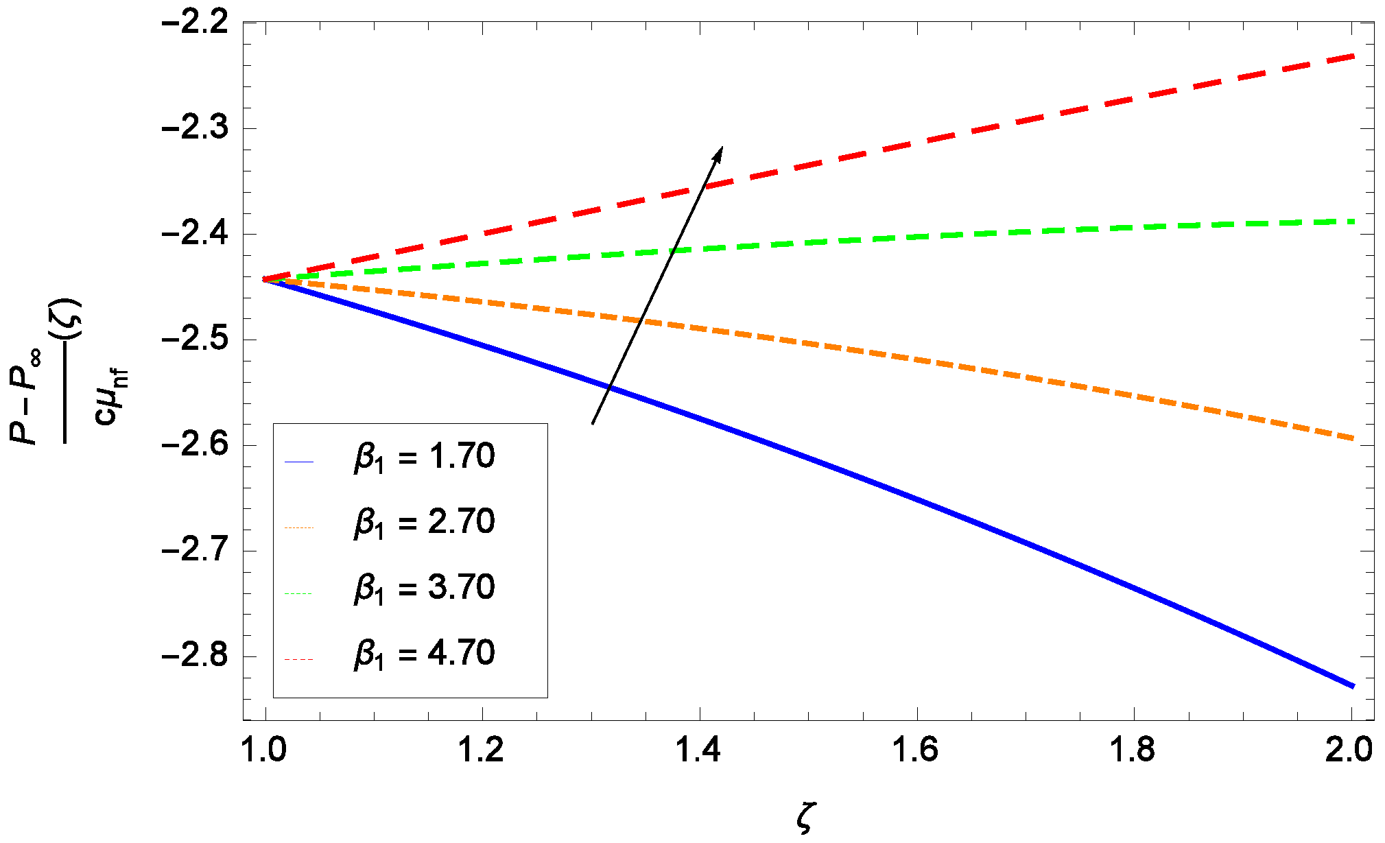
Figure 14.
Non-dimensional Pressure (ζ) sketch for h = −1.10, = 1.70, M = 0.10, Re = 0.70, Pr = 6.80 and various values of (CuO-HO).
Figure 14.
Non-dimensional Pressure (ζ) sketch for h = −1.10, = 1.70, M = 0.10, Re = 0.70, Pr = 6.80 and various values of (CuO-HO).
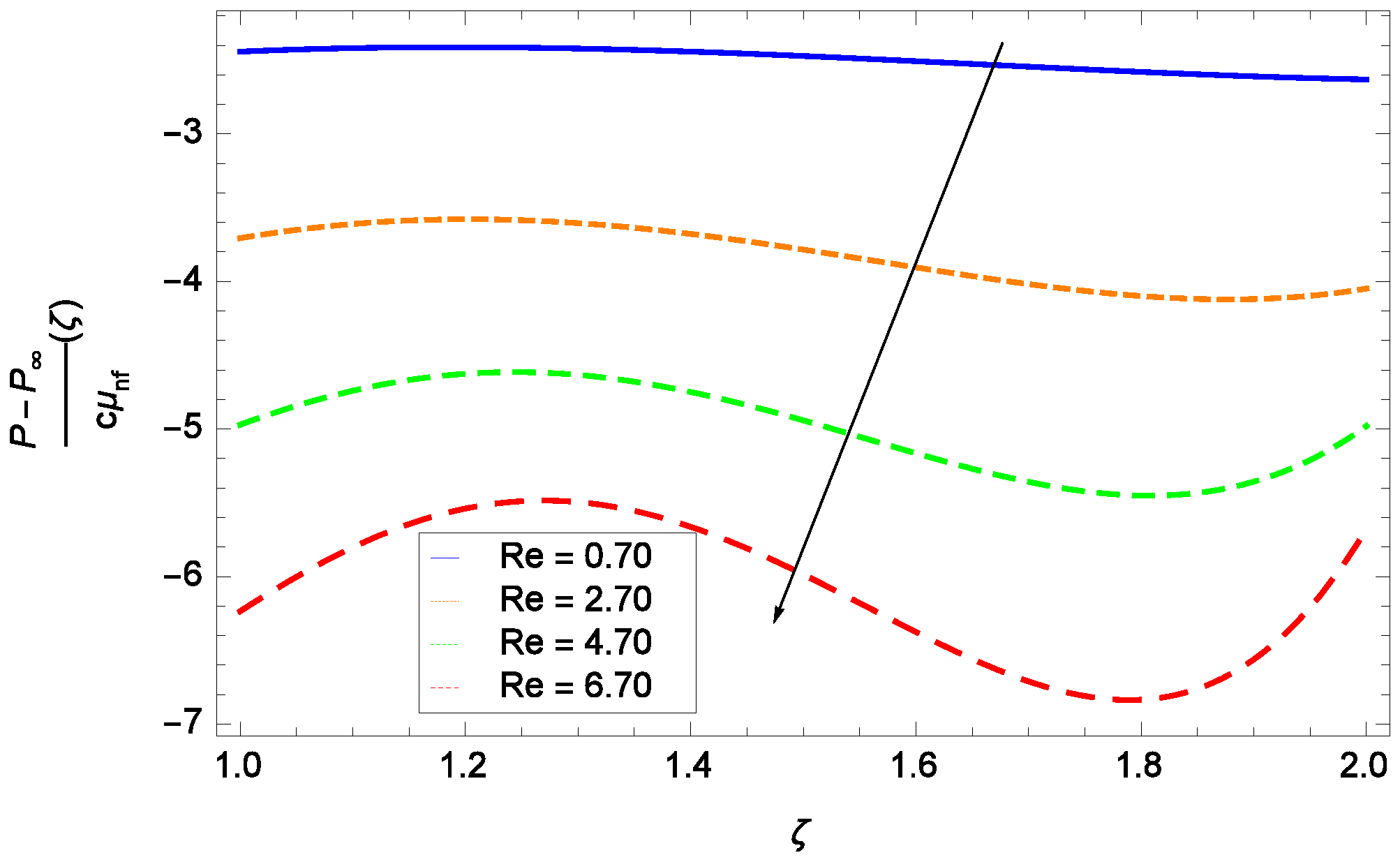
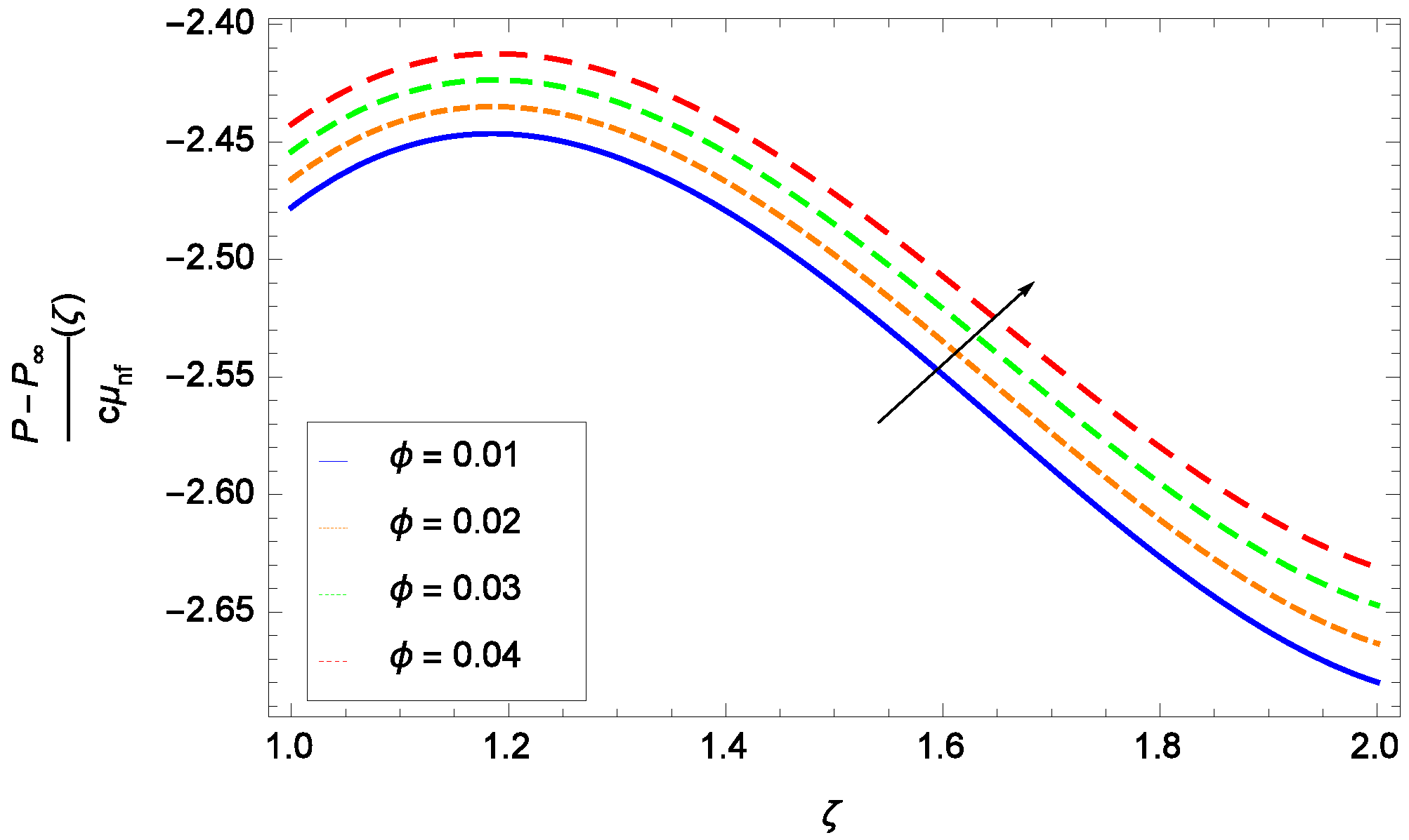
Figure 15.
Non-dimensional Pressure (ζ) sketch for h = −1.10, = 1.70, M = 0.10, = 0.04, Pr = 6.80 and greater quantities of Re (CuO-HO).
Figure 15.
Non-dimensional Pressure (ζ) sketch for h = −1.10, = 1.70, M = 0.10, = 0.04, Pr = 6.80 and greater quantities of Re (CuO-HO).
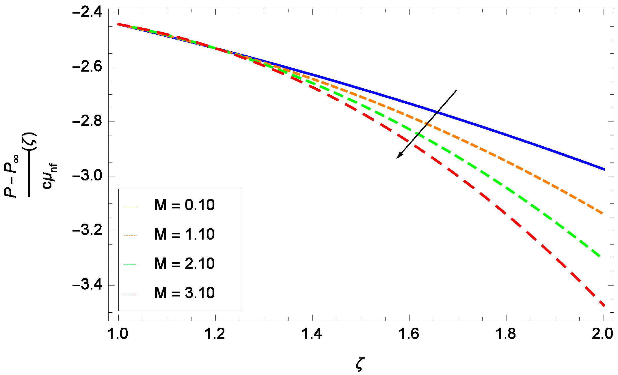
Figure 16.
Non-dimensional Pressure (ζ) sketch for h = −0.10, = 1.70, M = 0.10, Re = 0.70, = 0.04, Pr = 6.80 and greater quantities of M (CuO-HO).
Figure 16.
Non-dimensional Pressure (ζ) sketch for h = −0.10, = 1.70, M = 0.10, Re = 0.70, = 0.04, Pr = 6.80 and greater quantities of M (CuO-HO).
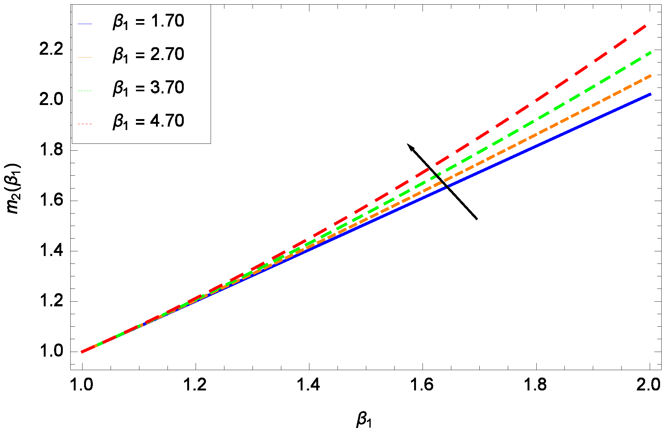
Figure 17.
Rate of spray m() sketch for h = 0.10, M = 0.10, Re = 0.70, = 0.04, Pr = 6.80 and various values of (CuO-HO).
Figure 17.
Rate of spray m() sketch for h = 0.10, M = 0.10, Re = 0.70, = 0.04, Pr = 6.80 and various values of (CuO-HO).
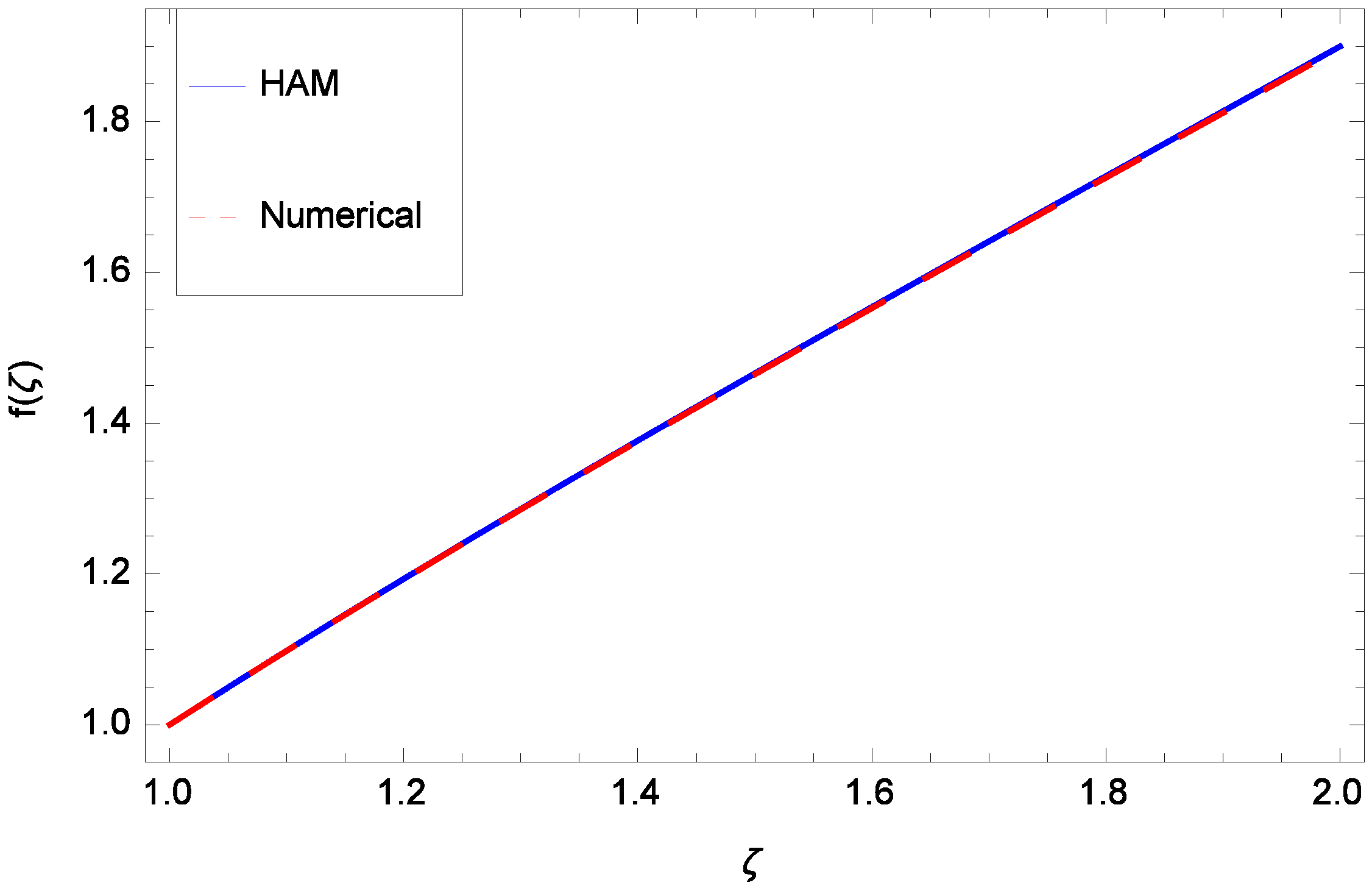
Figure 18.
Comparison of the velocity solution of HAM with numerical method solution when h = −0.55, = 2.00, M = 0.10, Re = 0.70, = 0.04, Pr = 1.10 for (CuO-HO).
Figure 18.
Comparison of the velocity solution of HAM with numerical method solution when h = −0.55, = 2.00, M = 0.10, Re = 0.70, = 0.04, Pr = 1.10 for (CuO-HO).
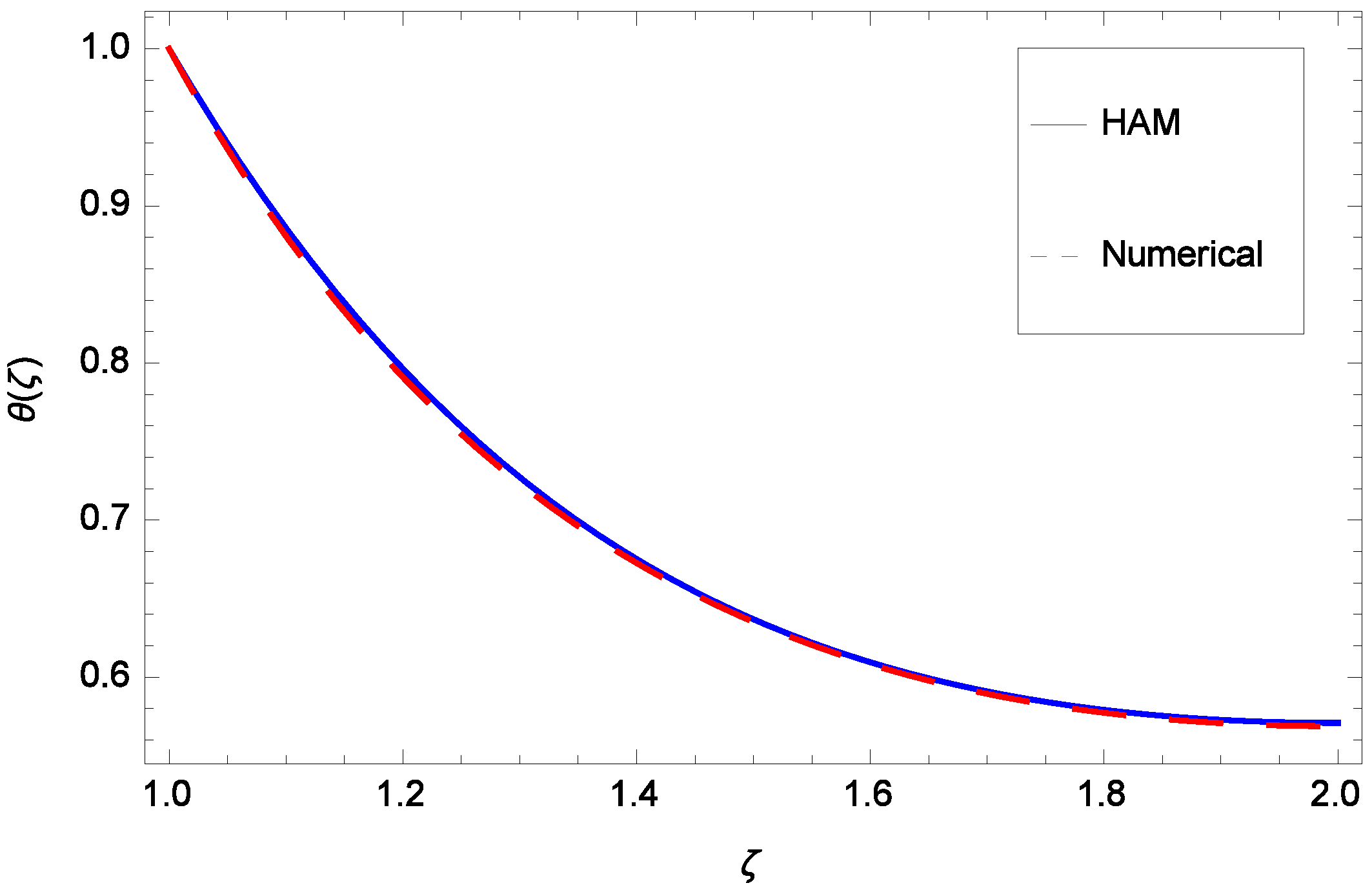
Figure 19.
Comparison of the temperature solution of HAM with numerical method solution when h = −0.55, = 2.00, M = 0.10, Re = 0.70, = 0.04, Pr = 1.10 for (CuO-HO).
Figure 19.
Comparison of the temperature solution of HAM with numerical method solution when h = −0.55, = 2.00, M = 0.10, Re = 0.70, = 0.04, Pr = 1.10 for (CuO-HO).
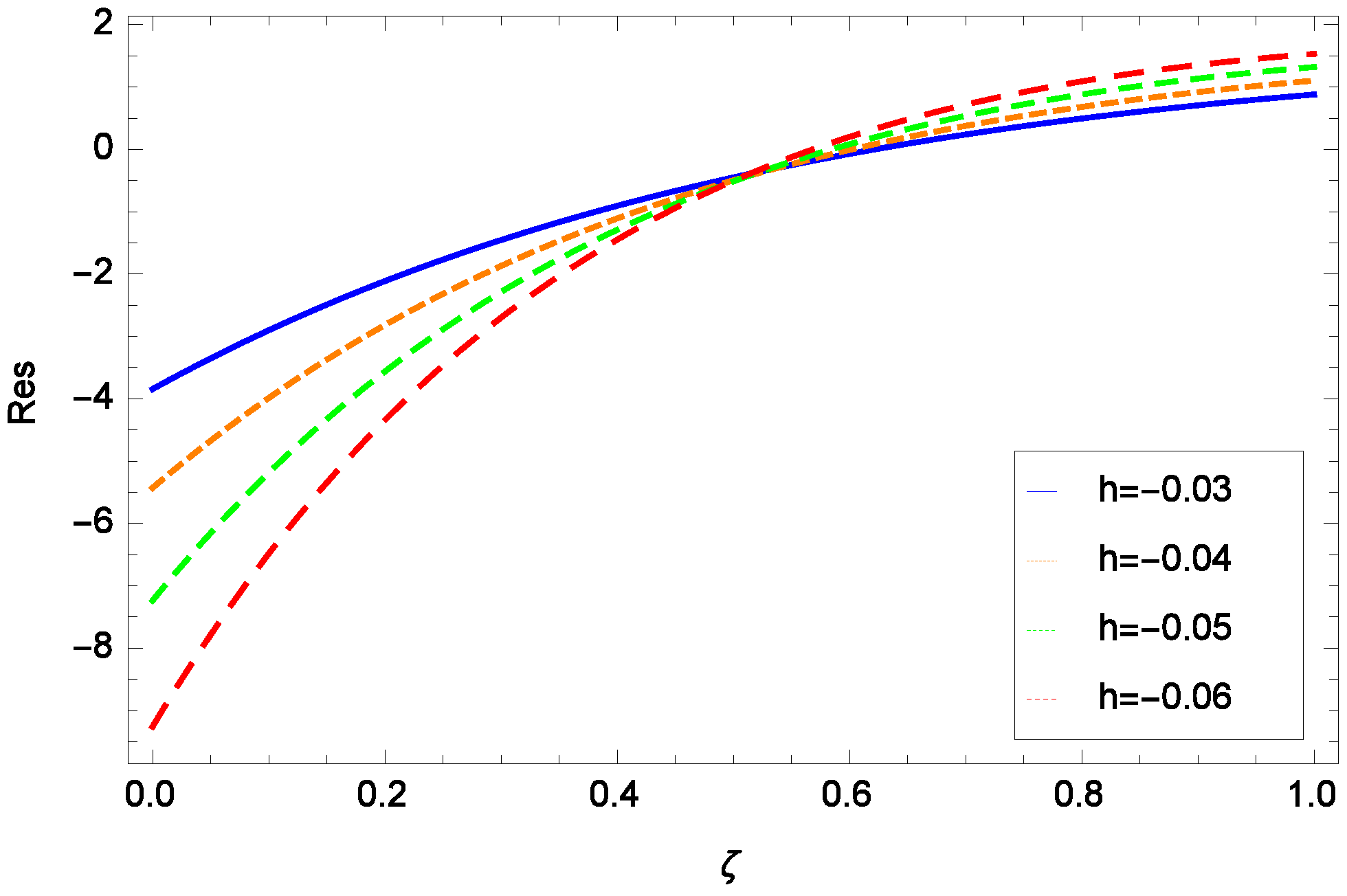
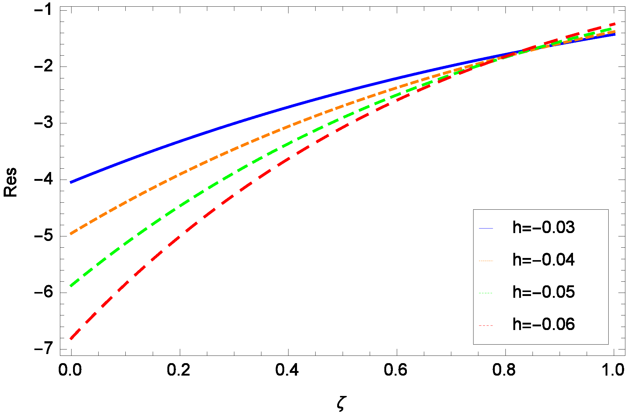
Figure 20.
Residual errors sketch of the velocity solution of HAM when = 2.00, M = 0.10, Re = 0.70, = 0.04, Pr = 1.10 and various values of h for (CuO-HO).
Figure 20.
Residual errors sketch of the velocity solution of HAM when = 2.00, M = 0.10, Re = 0.70, = 0.04, Pr = 1.10 and various values of h for (CuO-HO).
Figure 21.
Residual errors sketch of the temperature solution of HAM when = 2.00, M = 0.10, Re = 0.70, = 0.04, Pr = 1.10 and various values of h for (CuO-HO).
Figure 21.
Residual errors sketch of the temperature solution of HAM when = 2.00, M = 0.10, Re = 0.70, = 0.04, Pr = 1.10 and various values of h for (CuO-HO).
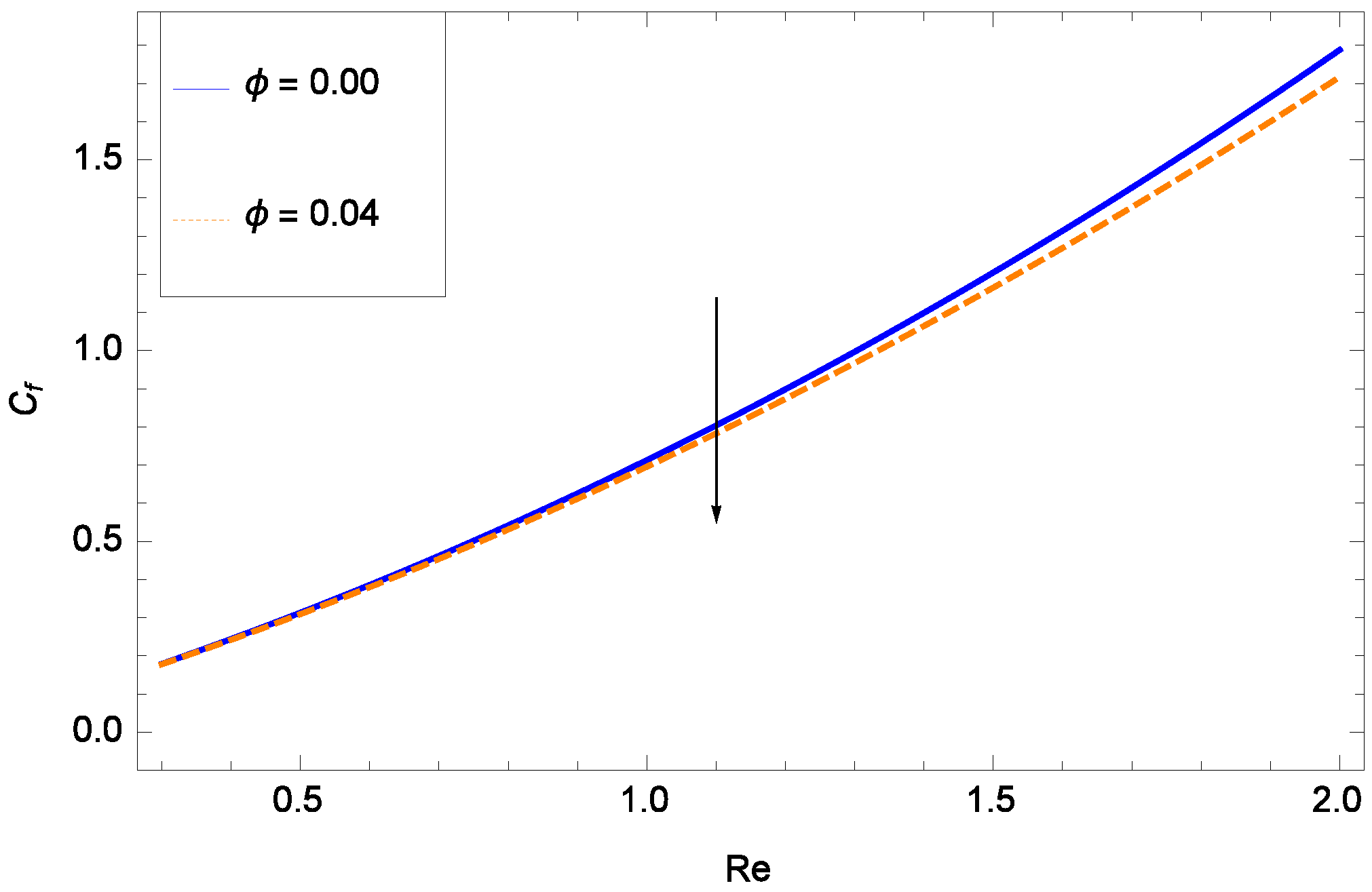
Figure 22.
Skin friction coefficient (C) when h = −0.40, = 2.00, M = 0.10, Pr = 6.80 and various values of against Reynolds number Re for (CuO-HO).
Figure 22.
Skin friction coefficient (C) when h = −0.40, = 2.00, M = 0.10, Pr = 6.80 and various values of against Reynolds number Re for (CuO-HO).
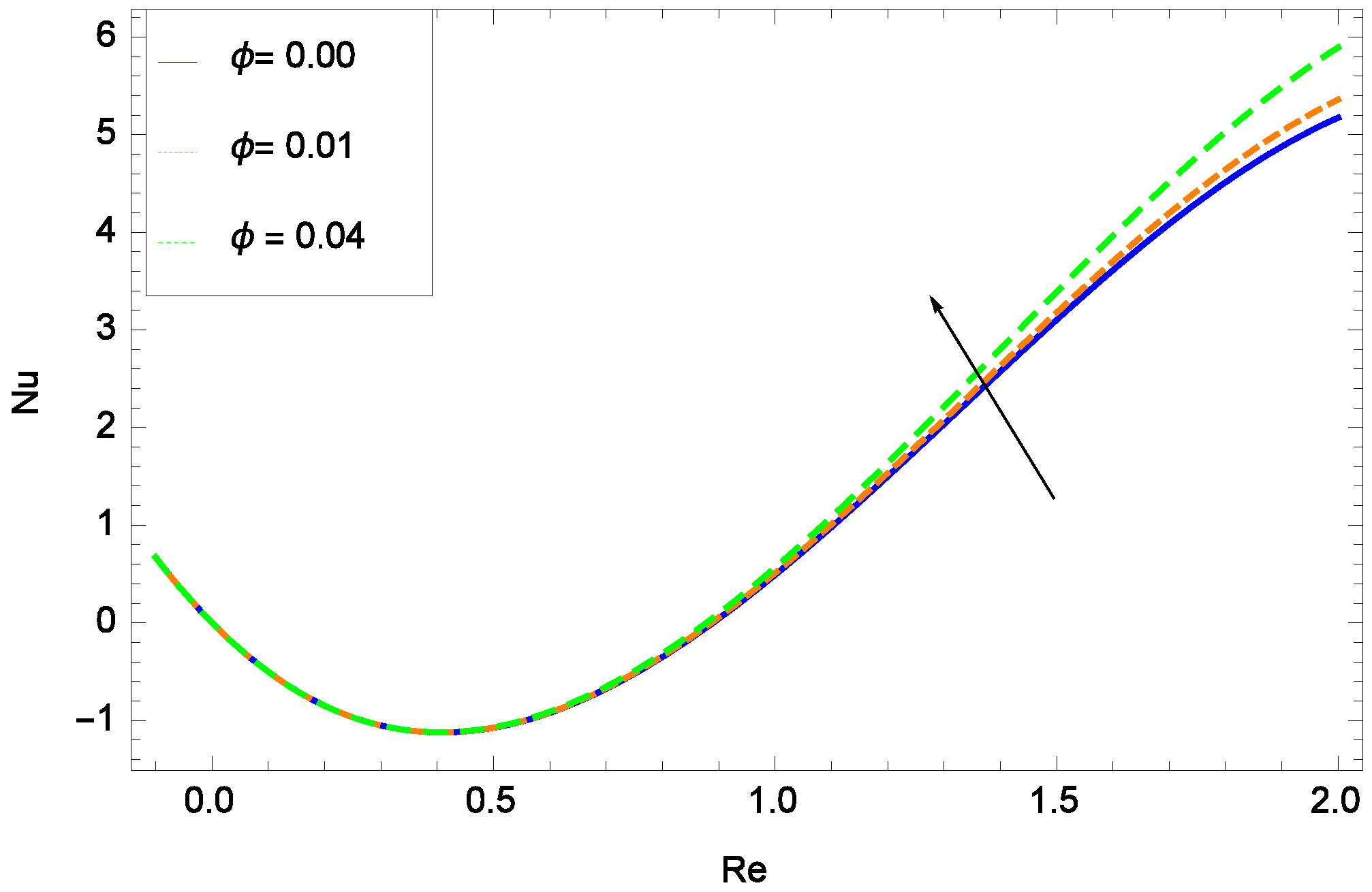
Figure 23.
Nusselt number (Nu) when h = −0.40, = 0.10, M = 0.10, Pr = 6.80 and various values of against Reynolds number Re for (CuO-HO).
Figure 23.
Nusselt number (Nu) when h = −0.40, = 0.10, M = 0.10, Pr = 6.80 and various values of against Reynolds number Re for (CuO-HO).
Table 1.
Thermophysical quantities of water and nanoparticles [
47].
Table 1.
Thermophysical quantities of water and nanoparticles [47].
| Thermophysical Quantities | Pure Water | AlO | CuO |
|---|
| ρ(Kg/m) | 997.1 | 3970 | 6500 |
| C(J/KgK) | 4179 | 765 | 540 |
| K(W/mk) | 0.613 | 25 | 18 |
| d(nm) | - | 47 | 29 |
| σ(Ωm) | 0.05 | 10 | 10 |
Table 2.
Coefficients values of the Al
O
-H
O and CuO-H
O [
47].
Table 2.
Coefficients values of the AlO-HO and CuO-HO [47].
| Coefficients Values | AlO-HO | CuO-HO |
|---|
| c | 52.813488759 | −26.593310846 |
| c | 6.115637295 | −0.403818333 |
| c | 0.6955745084 | −33.3516805 |
| c | 4.17455552786 × 10 | 1.915825591 |
| c | 0.176919300241 | 6.42185846658 × 10 |
| c | −298.19819084 | 48.40336955 |
| c | −34.532716906 | −9.787756683 |
| c | −3.9225289283 | 190.245610009 |
| c | −0.2354329626 | 10.9285386565 |
| c | −0.999063481 | −0.72009983664 |
Table 3.
Comparison of solution of HAM with numerical method solution.
Table 3.
Comparison of solution of HAM with numerical method solution.
| Velocity | Temperature |
|---|
| f() | Numerical Values | Errors | | () | Numerical Values | Errors |
| 0.0 | 1. | 1. | −4.44089 × 10 | 0.0 | 1.0 | 1.0 | −6.30818 ×10 |
| 0.1 | 1.09826 | 1.09814 | 0.000124947 | 0.1 | 0.885877 | 0.880696 | 0.00518123 |
| 0.2 | 1.19347 | 1.19308 | 0.000389778 | 0.2 | 0.7963263 | 0.79091 | 0.00541687 |
| 0.3 | 1.2862 | 1.28551 | 0.000692582 | 0.3 | 0.7273 | 0.723303 | 0.00399767 |
| 0.4 | 1.37694 | 1.37595 | 0.000987247 | 0.4 | 0.675195 | 0.672662 | 0.00253345 |
| 0.5 | 1.46611 | 1.46485 | 0.0012588 | 0.5 | 0.636847 | 0.635206 | 0.00164092 |
| 0.6 | 1.5541 | 1.55259 | 0.00150777 | 0.6 | 0.609527 | 0.608145 | 0.00138164 |
| 0.7 | 1.64121 | 1.63947 | 0.0017406 | 0.7 | 0.590937 | 0.589388 | 0.00154869 |
| 0.8 | 1.72772 | 1.72575 | 0.00196426 | 0.8 | 0.579203 | 0.577345 | 0.00185881 |
| 0.9 | 1.81386 | 1.81167 | 0.00218373 | 0.9 | 0.572877 | 0.570793 | 0.002084 |
| 1.0 | 1.89982 | 1.89742 | 0.00240171 | 1.0 | 0.570928 | 0.568784 | 0.00214339 |
Table 4.
Results achieved by HAM and Residual Errors.
Table 4.
Results achieved by HAM and Residual Errors.
| Velocity | Temperature |
|---|
| f() | Residual Errors | | () | Residual Errors |
| 0.0 | 1. | −0.64363 | 0.0 | 1.0 | 1.53209 |
| 0.1 | 1.09667 | −0.456915 | 0.1 | 0.931831 | 1.64776 |
| 0.2 | 1.18735 | −0.29789 | 0.2 | 0.875176 | 1.71672 |
| 0.3 | 1.27298 | −0.162766 | 0.3 | 0.828685 | 1.75179 |
| 0.4 | 1.35444 | −0.0481967 | 0.4 | 0.791164 | 1.76305 |
| 0.5 | 1.43248 | 0.0487658 | 0.5 | 0.761557 | 1.75834 |
| 0.6 | 1.50783 | 0.130716 | 0.6 | 0.738932 | 1.74376 |
| 0.7 | 1.58112 | 0.199934 | 0.7 | 0.722468 | 1.72407 |
| 0.8 | 1.65293 | 0.258415 | 0.8 | 0.711444 | 1.70297 |
| 0.9 | 1.72381 | 0.307909 | 0.9 | 0.705227 | 1.6833 |
| 1.0 | 1.79423 | 0.349941 | 1.0 | 0.703266 | 1.6673 |
Table 5.
Comparison of the effects of different kinds of nanoparticles on skin friction coefficient () as a function of Reynolds number Re when = 0.04.
Table 5.
Comparison of the effects of different kinds of nanoparticles on skin friction coefficient () as a function of Reynolds number Re when = 0.04.
| Parameter | Sheikhoeslami [45] | Sheikhoeslami [45] | Present Study (When h = −0.20, = 0.50, M = 0.10, Pr = 6.80) |
|---|
| Re | CuO | AlO | CuO |
| 0.1 | 0.679741 | 0.703897 | 0.577056 |
| 1 | 1.194617 | 1.224377 | 0.215528 |
| 2 | 1.579317 | 1.615502 | 0.384453 |
Table 6.
Comparison of the effects of different kinds of nanoparticles on Nusselt number (Nu) as a function of Reynolds number Re when = 0.04.
Table 6.
Comparison of the effects of different kinds of nanoparticles on Nusselt number (Nu) as a function of Reynolds number Re when = 0.04.
| Parameter | Sheikhoeslami [45] | Sheikhoeslami [45] | Present Study (When h = −0.40, = 0.10, M = 0.10, Pr = 6.80) |
|---|
| Re | CuO | AlO | CuO |
| 0.1 | 1.846686 | 1.70097 | 0.227864 |
| 1 | 4.324278 | 4.113995 | 2.25099 |
| 2 | 5.996721 | 5.711652 | 4.40516 |


 ,
, 


