
A New Engine Fault Diagnosis Method Based on Multi-Sensor Data Fusion


School of Electronics and Information, Northwestern Polytechnical University, Xi’an 710072, Shaanxi, China
*
Author to whom correspondence should be addressed.
Appl. Sci. 2017, 7(3), 280; https://doi.org/10.3390/app7030280
Submission received: 29 January 2017
/
Revised: 1 March 2017
/
Accepted: 9 March 2017
/
Published: 14 March 2017
Abstract
:Fault diagnosis is an important research direction in modern industry. In this paper, a new fault diagnosis method based on multi-sensor data fusion is proposed, in which the Dempster–Shafer (D–S) evidence theory is employed to model the uncertainty. Firstly, Gaussian types of fault models and test models are established by observations of sensors. After the models are determined, the intersection area between test model and fault models is transformed into a set of BPAs (basic probability assignments), and a weighted average combination method is used to combine the obtained BPAs. Finally, through some given decision making rules, diagnostic results can be obtained. The proposed method in this paper is tested by the Iris data set and actual measurement data of the motor rotor, which verifies the effectiveness of the proposed method.
1. Introduction
Engine fault diagnosis, one of the aspects of fault diagnosis [1,2], which is useful for engine design [3,4], can make the maintenance personnel quickly grasp the engine fault type and make the corresponding maintenance measures. At present, there are many methods for fault diagnosis. For example, the methods based on expert systems [5,6,7], which utilize the experience accumulated by domain experts in long-term practice. In these kinds of methods, a computer program is designed to simulate the reasoning and decision-making process of human experts to diagnose faults. Other fault diagnosis methods, such as machine learning [8,9] and signal processing [10,11,12], where there is a comparison of frequency analysis and SVM (support vector machine) classifiers in [11,12], are also widely used in practical applications [13,14]. There are also fault diagnosis methods in multi-sensor networks. As another efficient method to fault diagnosis, the residual-based unsupervised fault diagnosis method addresses uncertainty in the form of error bars around the soft computing models extracted from data [15,16,17]. Multi-sensor data fusion fault diagnosis [18,19], which is widely used in sensor design [20,21], as a data-driven approach, has been paid more and more attention. The advantages of multi-sensor data fusion for fault diagnosis can be concluded as follows:
- Compared with single source data, multi-source information fusion or multi-sensor information fusion can improve the accuracy and promptness of fault diagnosis.
- Multi-sensor data fusion method has the ability to deal with the uncertainty of data in fault diagnosis so as to enhance the credibility of diagnostic results.
A number of theories have been developed on multi-sensor data fusion, such as the Dempster–Shafer (D–S) evidence theory [22,23,24,25,26], fuzzy set theory [27], rough sets theory [28,29], Z numbers [30,31], and D numbers [32,33,34,35]. The D–S evidence theory, first proposed by Dempster [22] and then developed by Shafer [23], is able to deal with uncertain information without a prior probability. It has been applied to wide areas, such as decision making [36,37,38], pattern recognition [39,40,41] and risk assessment [42,43,44,45]. In the D–S evidence theory, mass function (or basic probability assignment (BPA)), belief function and plausibility function are defined to express uncertain information. Many methods can be used to integrate multi-source information [46,47,48], while Dempster’s combination rule, which is effective at addressing uncertainty information, can be used to fuse multi-source information in uncertain environments to make a decision.
Much research have been carried out in fault diagnosis based on multi-sensor data fusion [31,49,50,51,52]. Generally, the overall process of fault diagnosis based on multi-sensor data fusion is as follows. Firstly, prior to diagnosis, fault models are established using features extracted from known faulty equipment. Secondly, test models are established using the extracted features from a machine to be detected. Thirdly, BPAs are obtained by computing the BPA determination algorithm using the obtained fault models and test models. Finally, final BPA is obtained by using a combination rule to fuse all of the obtained BPAs. Decision making is carried out through the obtained final BPA. In this process, the key issues are the reasonable establishment of models and the reasonable determination of BPA. However, in previous studies, they are not well solved, especially considering the uncertainty. For example, in [31], the authors take ordinates of intersection points of functions as BPA, while it is not enough to express the uncertain information in fault models due to inadequate consideration on model variance information. Xu [53] utilized the relationship between test data and the Gaussian distribution model generated by training data to determine BPA, while using single measurement data as test data may fail in addressing uncertainty when the fluctuation of sensor data is large. Hégarat-Mascle et al. [54] and Salzenstein et al. [55] modeled the knowledge provided by each information source using probability density functions, while the mass value associated with each compound hypothesis is obtained by subtracting the mass values of the involved individual hypotheses. In this paper, a new fault diagnosis method based on multi-sensor data fusion is proposed. In the step of modeling, for both fault models and test models, considering the Gaussian type interference of mechanical noise and electromagnetic waves in sensor working environments, the Gaussian type membership function is established as the model. The proposed modeling method matches measured data of sensor well. In the step of BPA determination, the intersection area between model curves under the identical attribute is transformed into a set of BPA. The proposed BPA determination method, which fully utilize the variance information of models, can better express uncertain information. In the step of BPA combination and decision making, a weighted average approach for evidence combination [56] is used to combine the obtained BPAs and multiple criteria are established for decision making. The proposed method establishes reasonable fault models and test models based on the complex working environment of sensors and takes into account the variance information of the model, which can better express the uncertain information in the system and improve the reliability of the fault diagnosis.
The paper is organized as follows: in Section 2, the preliminaries are briefly introduced. In Section 3, a new fault diagnosis method based on multi-sensor data fusion is proposed. The proposed method is used for Iris data set classification and engine fault diagnosis in Section 4. Conclusions are made in Section 5.
2. Preliminaries
2.1. Dempster–Shafer Evidence Theory
The D–S evidence theory [22,23], as introduced by Dempster and then developed by Shafer, has emerged from their works on statistical inference and uncertain reasoning. This theory is widely used in decision making [57,58,59,60,61] and information fusion [62,63,64,65]. In this part, a few concepts about D–S evidence theory are given.
Let Θ be a finite nonempty set of mutually exclusive alternatives and Θ is called the frame of discernment
The power set of Θ is indicated by , namely:
For a frame of discernment Θ, a basic probability assignment (BPA) is a mapping m from to [0,1], formally defined by
which satisfies the following condition:
The mass represents how strongly the evidence support A. A is called a focal element when .
Two BPAs and can be combined with Dempster’s combination rule as follows:
where K is a normalization constant, reflecting the conflict between the two BPAs and .
For the sake of understanding, an illustrative example is given as follows to show how to combine two BPAs according to Equations (6) and (7).
Example 1.
Assuming , computational method of K and is as follows:
2.2. Evidence Distance
Jousselme [66] proposed the concept of evidence distance to measure the distance of BPAs. Let and be two BPAs on the frame of discernment Θ, containing N mutually exclusive and exhaustive hypotheses. The distance between and is defined as
where and are the BPAs according to Equations (4) and (5) and is a matrix whose elements are .
2.3. Weighted Average Approach for Evidence Combination
In the D–S evidence theory, Dempster’s combination rule is used to fuse certain multi-source information to make a decision. However, if there is a high level of conflict between evidence, the combination rule will fail [67]. Many methods were proposed to solve this problem [66,68,69,70]. Among them, Murphy [71] proposed a simple average approach to solve the problem. However, in Murphy’s approach, all bodies of evidence are equally important. Hence, a weighted average approach [56] was proposed to improve Murphy’s approach. The weighted average approach is given as follows.
Suppose the distance between two BPAs and is calculated and denoted as . The similarity measure between and is defined as:
If n BPAs need to be combined, the support degree of BPA is defined as:
Then, the credibility degree of the BPA is calculated as follows:
The credibility degree is actually a weight that shows the relative importance of the collected evidence. According to , the weighted average of the evidence MAE is obtained:
Finally, the weighted average evidence is combined n-1 times by using Dempster’s combination rule:
The obtained is the combination result of the n BPAs.
3. The Proposed Method for Fault Diagnosis
In this paper, a new multi-sensor data fusion method is proposed for fault diagnosis, and the detailed description of the proposed method is shown in Figure 1. One or more attribute features, which can be used for fault diagnosis, can be extracted from each sensor signal. Firstly, in step 1 of Figure 1, Gaussian types of fault models are established using the extracted attribute features from the signal of sensors in each known type of fault equipment. In step 2, Gaussian types of test models are generated as well using the attribute features extracted from sensor signals of the equipment. In step 3, the produced fault models and test models are matched to produce the BPAs. Finally, in step 4, the weighted average approach is used to combine the produced BPAs. Through the decision making rules, the diagnostic results that the equipment is working properly or which type of fault the equipment has is diagnosed. If the equipment has a type of fault, corresponding intervention measures will be implemented.
3.1. Fault Model Modeling
In this section, we give the method to determine the fault model. Due to the change of time and environment of the sensor measurements, the measured data have a certain degree of fuzziness. The membership function can be used to represent the fault features extracted from the observed data.
Suppose X is a sample space of a type of attribute feature variable extracted from the sensor—for example, the amplitude of fundamental harmonic in the frequency spectrum of sensor signal, the membership function of fault model can be modeled as:
where represents the membership function of fault F under the corresponding attribute.
Two main factors are considered in the determination of membership function: the working performance of the sensor itself such as the linearity of sensor measurements and various kinds of interferences in the working process of the sensor such as the interference of mechanical noise and electromagnetic waves. If only the second factor is considered, the probability density function of the measured value of the same physical quantity is generally regarded as a form of Gaussian distribution. Gaussian distribution possesses the following advantages [72]: first, the Gaussian distribution is manageable, that is, a large number of data that is related to Gaussian distribution can be put through it to obtain a exact form. Second, if the error can be seen as superposition of many independent random variables. According to the central limit theorem, the error is supposed to have the form of Gaussian distribution. Third, Gaussian distribution has an extremely wide range of practical background, and a lot of the probability distribution of random variables in production and scientific experiments can be approximately described by Gaussian distribution. We take the Gaussian type of membership function as a fault model based on the above several points, and the details of membership function determination are presented as follows:
- Assuming n groups of data are observed, each group consists of m consecutive observations in the same time interval . In order to make the generated fault model representative, n should be more than 3 and 30, respectively, and n groups of data should be observed at different times.
- Calculate the mean value μ and standard deviation σ of the n groups’ observations. Here, observation i in group j is denoted as . The mean value μ and standard deviation σ can be obtained as:
- The Gaussian type of membership function is obtained as:
3.2. Test Model Modeling
In fault diagnosis, considering the influences of the interferences in the working environment of the sensor, it is difficult to judge the fault class precisely from a single measurement. When multiple measurements on the equipment in the same time interval are obtained, the Gaussian type membership function can be obtained using Equations (15)–(17), which is denoted as:
is taken as a test model. Compared with the single measurement and mean value of multiple measurements, it is more comprehensive and objective to reflect the change of the value of equipment fault characteristic parameters.
3.3. BPA Determination
The determination of BPA is a key step in the application of D–S evidence theory. In the application of data fusion based on D–S evidence theory, the BPAs generated from different attributes will be combined to make a decision. While how to determine BPA from multi-sensor data fusion system is still an open issue, much research has been carried out [53,73]. The BPA determination method in [53] utilized the relationship between test data and Gaussian distribution model generated by training data. However, the method of determining BPA with single measurement values can not cover the fuzziness of sensors in complex working environments. Taking this fact into consideration, a BPA determination method based on multiple measurements value is proposed in this section.
Assuming the equipment in Figure 1 may have M faults occur, a total of N (N >L) attributes are extracted from L sensors. The frame of discernment should be . For a certain attribute k (k = 1, 2, ...,N), the test model under attribute k is put into its corresponding M fault models under attribute k to determine .
Let , , be the function curve, mean value, standard deviation of generated model of fault (i = 1, 2, 3, ..., M) under attribute k, respectively. Let , , be the function curve, mean value and standard deviation of generated model using observation under attribute k, respectively. The calculation procedures are as the following: the proposition support degree calculation method is given in Section 3.3.1, Section 3.3.2 and Section 3.3.3. is obtained by normalizing all obtained support degrees to propositions, which is shown in Section 3.3.4.
3.3.1. Support Degree Calculation of Singleton Propositions
In this part, the support degree of the test model to proposition denoted as (i = 1, 2, ..., M) is obtained.
Taking into account the property of the model curve, firstly let us calculate the integral interval:
Then, the intersection area between the test model curve and the fault model curve is calculated:
For example, is as shown in Figure 2a if .
Finally, calculate the support degree of the test model to proposition :
where the is the area under the test model curve , .
3.3.2. Support Degree Calculation of Propositions with Two Elements
In this part, the support degree of the test model to compound proposition denoted as () ( = 1, 2, ..., < j) is obtained.
Considering the nature of the model curve, firstly let us calculate the integral interval:
Then, the intersection area between the test model curve and the fault model curves is calculated:
For example, is as shown in Figure 2b if .
Finally, the support degree of the test model to compound proposition is obtained:
where the is the area under the test model curve , .
3.3.3. Support Degree Calculation of Propositions with Multiple Elements
In this part, the support degree of the test model to compound proposition denoted as is obtained.
Taking into account the nature of the model curve, firstly let us calculate the integral interval:
Then, the intersection area between the test model curve and the fault model curves is obtained as:
For example, is as shown in Figure 2c if .
Finally, the support degree of the test model to compound proposition is obtained:
where the is the area under the test model curve , .
3.3.4. Normalization
The sum of all obtained support degrees is denoted as .
The obtained support degrees are normalized to obtain under attribute k:
3.4. BPA Combination and Decision Making
After are obtained through the method in Section 3.3, these N BPAs can be combined using Equations (8)–(12) to obtain final BPA. Decision making rules based on BPA are required because it is a set of BPA ultimately obtained through the fault diagnosis method based on multi-sensor data fusion. Hence, the decision making rules based on the obtained final BPA in this paper are as follows. If is the final diagnostic fault class of the equipment, the following decision making rules should be simultaneously met:
- should have the maximum belief in final BPA that is (i = 1, 2, ..., M) and should exceed a threshold . is the minimum belief of . should be a slightly larger value to ensure the high credibility of diagnostic result so as to make sure the correctness of diagnostic result. Here, is designated as 0.5. The purpose of this rule is to make the reliability of the diagnostic result sufficiently large.
- The BPA of dual set proposition and multi-subset proposition, such as , , , should be less than a certain threshold . is the maximum belief of the uncertain components. If larger than , it is considered that the uncertainty of diagnostic result is too large, which may lead to the wrong diagnostic result. should be a smaller value so that the uncertainty of the diagnostic result is small. Here, is designated as 0.3. The purpose of this rule is to make the uncertainty of the diagnostic result smaller.
- The difference between and should be larger than a certain threshold that is , where (i = 1, 2, ..., ). is minimum difference between the maximum and the second largest in (i = 1, 2, ..., M). If larger than , it is considered that the diagnostic result can be clearly distinguished from the credibility of the other fault types, which can avoid false diagnostic results. Hence, to avoid false diagnostic results, can not be too small. Here, is designated as 0.2 because that is too large may cause a missing alarm. The purpose of this rule is to make the difference between the maximum and the second largest in larger, which means that is relatively larger in (i = 1, 2, ..., M).
If such can not be found, it is considered that the decision making can not be made by the obtained final BPA. The above decision making rules are based on the same fundamental principle with traditional decision making methods based on BPA [74].
4. Applications
In this section, two examples are given to demonstrate the effectiveness of the proposed method. In the first example of Iris data set classification, which is similar to fault diagnosis, multiple instances are selected as the test set to simulate the selection of the test sample in fault diagnosis, and the identification accuracy is high. In the second application, the fault diagnosis experiment of a motor rotor is carried out to demonstrate the validity in engine fault diagnosis.
4.1. Iris Data Set Classification
The Iris data set [75], which is perhaps the best known database to be found in pattern recognition literature, involves classification of three species of the Iris flowers, Iris setosa (S), Iris versicolour (E), and Iris virginica (V) on the basis of four numeric attributes of the Iris flower: sepal length () in cm, sepal width () in cm, petal length () in cm, and petal width () in cm. The frame of discernment should be .
In the Iris data set, there are 50 instances for each of three species. The data are obtained from the UCI (University of California Irvine) Machine Learning Repository [76] of machine learning databases. Among 50 instances of each species, 20 instances are randomly selected as the training set; thus, there are a total of 12 training models (Table 1 and Figure 3). Ten instances are randomly selected in the rest of 30 instances under each attribute of E (Iris versicolour) as the test set; thus, there are a total of four test models (Table 1 and Figure 3). Each of the four attributes is regarded as an information source. The final identification result should be E (Iris versicolour).
First, calculate the support degrees, and the results are shown in Table 2. Then, the BPA of each attribute is obtained through the normalization of support degrees (Table 3). After that, using the combination method mentioned in Section 2.3, the final BPA is obtained (Table 3). Finally, through the decision making rules mentioned in Section 3.4, the final identification result is E (Iris versicolour).
Samples from S, E, and V were tested as test sets 10,000 times, respectively, and the accuracy of the method on Iris data set classification is presented in Table 4 using the decision method mentioned in Section 3.4. The overall recognition rate of the three categories is 99.98%.
4.2. Motor Rotor Fault Diagnosis
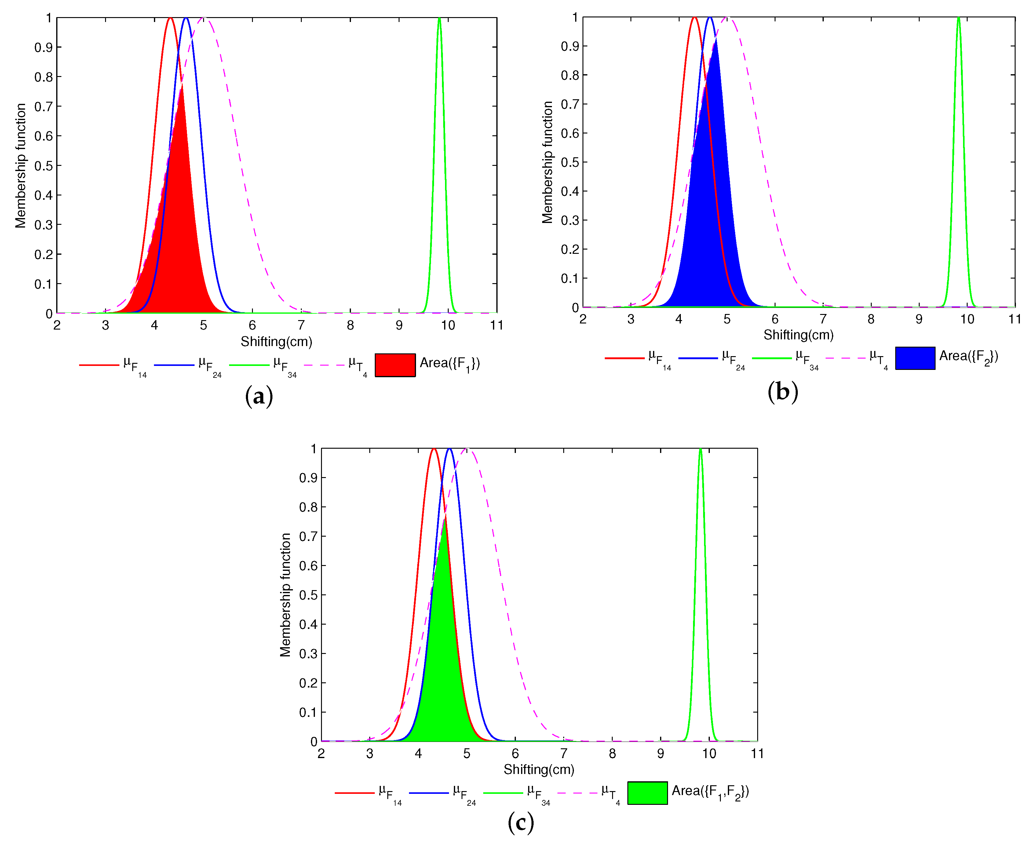
In this section, the proposed method is applied in practical engine fault diagnosis, and experimental data is from actual measurement data of the motor rotor [77]. Feature j under fault i is denoted as , where , respectively, on behalf of the three kinds of faults: rotor imbalance, rotor misalignment and the base loose. In addition, , respectively, on behalf of the four features: the amplitude of fundamental harmonic (), the amplitude of second harmonic (), and the amplitude of the third harmonic () in the frequency spectrum of the rotor vibration acceleration sensor signal and shifting of rotor vibration (). For example, means feature of fault rotor imbalance. The frame of discernment should be . There are five sets of measured data for specific i and j and each set of measured data is composed of forty continuous measurements in sixteen seconds.
Step 1: Establish fault models . For specific i and j, four sets of feature data are randomly selected as fault samples to generate fault model ; thus, a total of 12 fault models can be established for all i and j. For example, is shown in Table 5 and the function curve of is shown in Figure 4a.
Step 2: Generate test models . Assuming the left four sets of feature data in are selected as the test sample, which can be used to generate test models , the final diagnostic result should be . For example, is shown in Table 5 and the function curve of is shown in Figure 4b.
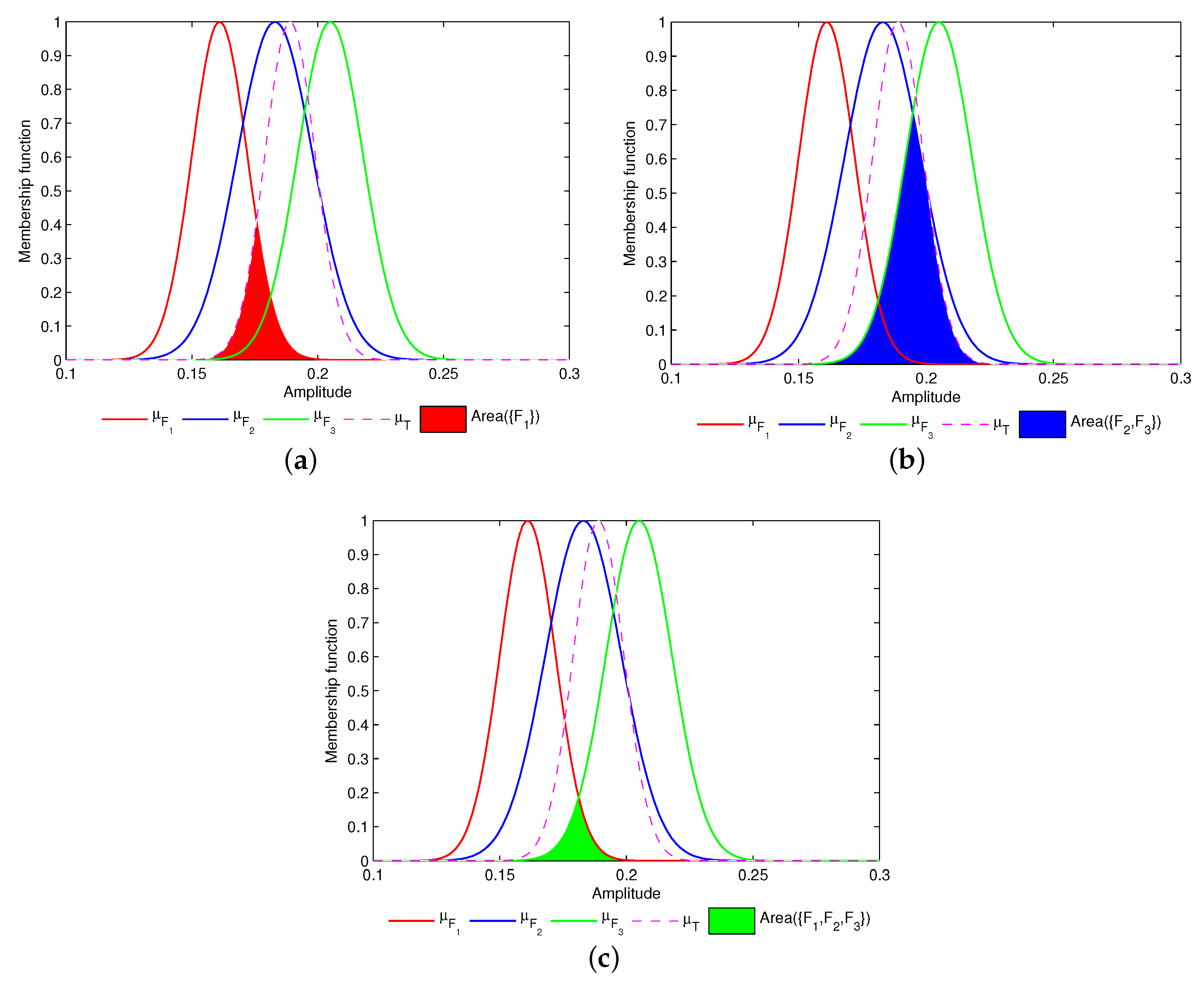
Step 3: Generate . After 12 fault models and four test models are obtained, the can be generated by matching the fault models with the test model . Taking test model as an example, a detailed introduction to the BPA generation process of is given as follows with graphical assistant instructions:
In Figure 5, first, the integral interval is calculated:
- For , the integral interval is (3.0740,6.9470).
- For , the integral interval is (3.0740,6.9470).
- For , the integral interval is (3.0740,6.9470).
Then, the intersection area between fault models and test model, which is represented by the shadow in Figure 5, is obtained as:
Third, the calculated support degrees are as follows:
, ,
Finally, normalizing the obtained support degrees, (BPA under feature 4 ()) is obtained as:
, ,
Step 4: Combine the obtained BPAs and give the result of diagnosis. Using the combination method mentioned in Section 3.4, the final BPA is obtained (Table 6). Through the decision making rules mentioned in Section 3.4, the final diagnostic result is fault (rotor misalignment).
Through five experiments, the experiment results of the proposed fault diagnosis method is presented in Table 7 using decision making rules mentioned in Section 3.4. The mean value and standard deviation of models in each case are as follows:
For case 1: , , , , , , , , , , , , , , , .
For case 2: , , , , , , , , , , , , , , , .
For case 3: , , , , , , , , , , , , , , , .
For case 4: , , , , , , , , , , , , , , , .
For case 5: , , , , , , , , , , , , , , , .
5. Conclusions
This paper presented a new fault diagnosis method based on multi-sensor data fusion. The Gaussian type of membership function is used to construct a fault model and a test model due to its advantages in processing sensor data. First, the distribution of the measurements of the sensor, which is working in a complex environment, is generally regarded as Gaussian distribution if the influence of the performance of the sensor is ignored. Second, the Gaussian type of membership function is tractable in dealing with a large number of data involving Gaussian distribution. The overall diagnostic processes are as follows: first, obtain the Gaussian type of fault models through a certain amount of fault samples. Secondly, through the measurements of sensors in equipment, Gaussian types of test models are determined. Thirdly, the intersection area between test models and fault models with identical attributes is transformed into a set of BPA. Finally, a weighted average approach is used to combine the obtained BPAs, and final diagnostic result is obtained through the proposed multiple decision making rules. On the whole, the proposed fault diagnosis method has the following advantages: the Gaussian type of fault model and test model determination method can fit the measurement data well due to the complex working environment of sensors in fault diagnosis. The basic probability assignment determination method based on the intersection area between the test model and fault models can better express uncertain information because this method takes into account the variance information of the models. Finally, the effectiveness of the proposed method is verified by some illustrative examples.
Acknowledgments
The work is partially supported by the National Natural Science Foundation of China (Grant No. 61671384), the Natural Science Basic Research Plan in Shaanxi Province of China (Program No. 2016JM6018), the Aviation Science Foundation (Program No. 20165553036), the Shanghai Aerospace Science and Technology Innovation Fund (Program No. SAST2016083), and the Seed Foundation of Innovation and Creation for Graduate Students in Northwestern Polytechnical University (Program No. Z2016122).
Author Contributions
Wen Jiang and Weiwei Hu conceived and designed the experiments; Wen Jiang performed the experiments; Chunhe Xie and Weiwei Hu analyzed the data; Chunhe Xie contributed analysis tools; and Weiwei Hu wrote the paper.
Conflicts of Interest
The authors declare no conflict of interest.
References
- Chen, J.; Patton, R.J. Robust Model-Based Fault Diagnosis for Dynamic Systems; Springer: New York, NY, USA, 1999. [Google Scholar]
- Isermann, R. Fault-Diagnosis Systems. An Introduction from Fault Detection to Fault Tolerance; Springer: New York, NY, USA, 2006; Volume 28, pp. 195–197. [Google Scholar]
- Al-Busaidi, W.; Pilidis, P. Modelling of the non-reactive deposits impact on centrifugal compressor aerothermo dynamic performance. Eng. Fail. Anal. 2016, 60, 57–85. [Google Scholar] [CrossRef]
- Xue, R.; Hu, C.; Sethi, V.; Nikolaidis, T.; Pilidis, P. Effect of steam addition on gas turbine combustor design and performance. Appl. Therm. Eng. 2016, 104, 249–257. [Google Scholar] [CrossRef]
- Ramesh, T.S.; Shum, S.K.; Davis, J.F. A structured framework for efficient problem solving in diagnostic expert systems. Comput. Chem. Eng. 1988, 12, 891–902. [Google Scholar] [CrossRef]
- Wu, J.D.; Wang, Y.H.; Bai, M.R. Development of an expert system for fault diagnosis in scooter engine platform using fuzzy-logic inference. Expert Syst. Appl. 2007, 33, 1063–1075. [Google Scholar] [CrossRef]
- Yang, J.B.; Liu, J.; Wang, J.; Sii, H.S.; Wang, H.W. Belief rule-base inference methodology using the evidential reasoning Approach-RIMER. IEEE Trans. Syst. Man Cybern. A Syst. Hum. 2006, 36, 266–285. [Google Scholar] [CrossRef]
- Tayarani-Bathaie, S.S.; Vanini, Z.S.; Khorasani, K. Dynamic neural network-based fault diagnosis of gas turbine engines. Neurocomputing 2014, 125, 153–165. [Google Scholar] [CrossRef]
- Tamilselvan, P.; Wang, P. Failure diagnosis using deep belief learning based health state classification. Reliab. Eng. Syst. Saf. 2013, 115, 124–135. [Google Scholar] [CrossRef]
- Yan, R.; Gao, R.X.; Chen, X. Wavelets for fault diagnosis of rotary machines: A review with applications. Signal Process. 2014, 96, 1–15. [Google Scholar] [CrossRef]
- Pichler, K.; Lughofer, E.; Pichler, M.; Buchegger, T.; Klement, E.P.; Huschenbett, M. Detecting cracks in reciprocating compressor valves using pattern recognition in the pV diagram. Pattern Anal. Appl. 2015, 18, 461–472. [Google Scholar] [CrossRef]
- Pichler, K.; Lughofer, E.; Pichler, M.; Buchegger, T.; Klement, E.P.; Huschenbett, M. Fault detection in reciprocating compressor valves under varying load conditions. Mech. Syst. Signal Process. 2016, 70–71, 104–119. [Google Scholar] [CrossRef]
- Fernando, H.; Surgenor, B. An unsupervised artificial neural network versus a rule-based approach for fault detection and identification in an automated assembly machine. Robot. Comput. Integr. Manuf. 2015, 43, 79–88. [Google Scholar] [CrossRef]
- Delgado-Arredondo, P.A.; Morinigo-Sotelo, D.; Osornio-Rios, R.A.; Avina-Cervantes, J.G.; Rostro-Gonzalez, H.; Romero-Troncoso, R.D.J. Methodology for fault detection in induction motors via sound and vibration signals. Mech. Syst. Signal Process. 2016, 83, 568–589. [Google Scholar] [CrossRef]
- Serdio, F.; Lughofer, E.; Pichler, K.; Buchegger, T.; Pichler, M.; Efendic, H. Fault detection in multi-sensor networks based on multivariate time-series models and orthogonal transformations. Inf. Fusion 2014, 20, 272–291. [Google Scholar] [CrossRef]
- Serdio, F.; Lughofer, E.; Zavoianu, A.C.; Pichler, K.; Pichler, M.; Buchegger, T.; Efendic, H. Improved Fault Detection employing Hybrid Memetic Fuzzy Modeling and Adaptive Filters. Appl. Soft Comput. 2017, 51, 60–82. [Google Scholar] [CrossRef]
- Serdio, F.; Lughofer, E.; Pichler, K.; Pichler, M.; Buchegger, T.; Efendic, H. Fuzzy Fault Isolation using Gradient Information and Quality Criteria from System Identification Models. Inf. Sci. 2015, 316, 18–39. [Google Scholar] [CrossRef]
- Mitchell, H.B. Multi-Sensor Data Fusion; Artech House: Norwood, MA, USA, 1990; pp. 585–610. [Google Scholar]
- Crowley, J.L. Principles and Techniques for Sensor Data Fusion; Springer: Berlin/Heidelberg, Germany, 1993; pp. 5–27. [Google Scholar]
- Alexandridis, A. Evolving RBF neural networks for adaptive soft-sensor design. Int. J. Neural Syst. 2013, 23, 1350029. [Google Scholar] [CrossRef] [PubMed]
- Graziani, S.; Pagano, F.; Xibilia, M.G. Soft sensor for a Propylene Splitter with seasonal variations. In Proceedings of the 2010 IEEE Instrumentation and Measurement Technology Conference (I2MTC), Austin, TX, USA, 3–6 May 2010; pp. 273–278.
- Dempster, A.P. Upper and lower probabilities induced by a multivalued mapping. Ann. Math. Stat. 1967, 38, 325–339. [Google Scholar] [CrossRef]
- Shafer, G. A mathematical theory of evidence. Technometrics 1976, 20, 242. [Google Scholar]
- Deng, X.; Xiao, F.; Deng, Y. An improved distance-based total uncertainty measure in belief function theory. Appl. Intell. 2017, in press. [Google Scholar] [CrossRef]
- Deng, X.; Han, D.; Dezert, J.; Deng, Y.; Shyr, Y. Evidence combination from an evolutionary game theory perspective. IEEE Trans. Cybern. 2016, 46, 2070–2082. [Google Scholar] [CrossRef] [PubMed]
- Jiang, W.; Zhan, J. A modified combination rule in generalized evidence theory. Appl. Intell. 2017. [Google Scholar] [CrossRef]
- Zadeh, L.A. Fuzzy sets. Inf. Control 1965, 8, 338–353. [Google Scholar] [CrossRef]
- Walczak, B.; Massart, D.L. Rough sets theory. Chemom. Intell. Lab. Syst. 1999, 47, 1–16. [Google Scholar] [CrossRef]
- Shen, L.; Tay, F.E.H.; Qu, L.; Shen, Y. Fault diagnosis using Rough Sets Theory. Comput. Ind. 2000, 43, 61–72. [Google Scholar] [CrossRef]
- Zadeh, L.A. A Note on Z-numbers. Inf. Sci. 2011, 181, 2923–2932. [Google Scholar] [CrossRef]
- Jiang, W.; Xie, C.; Zhuang, M.; Shou, Y.; Tang, Y. Sensor Data Fusion with Z-Numbers and Its Application in Fault Diagnosis. Sensors 2016, 16, 1509. [Google Scholar] [CrossRef] [PubMed]
- Zhou, X.; Shi, Y.; Deng, X.; Deng, Y. D-DEMATEL: A new method to identify critical success factors in emergency management. Saf. Sci. 2017, 91, 93–104. [Google Scholar] [CrossRef]
- Zhou, X.; Deng, X.; Deng, Y.; Mahadevan, S. Dependence assessment in human reliability analysis based on D numbers and AHP. Nucl. Eng. Des. 2017, 313, 243–252. [Google Scholar] [CrossRef]
- Deng, X.; Hu, Y.; Deng, Y.; Mahadevan, S. Supplier selection using AHP methodology extended by D numbers. Expert Syst. Appl. 2014, 41, 156–167. [Google Scholar] [CrossRef]
- Deng, X.; Lu, X.; Chan, F.T.; Sadiq, R.; Mahadevan, S.; Deng, Y. D-CFPR: D numbers extended consistent fuzzy preference relations. Knowl. Based Syst. 2015, 73, 61–68. [Google Scholar] [CrossRef]
- Yao, J.; Wu, C.; Xie, X.; Qian, K. A new method of information decision-making based on D–S evidence theory. In Proceedings of the IEEE International Conference on Systems Man and Cybernetics, Istanbul, Turkey, 10–13 October 2010; pp. 1804–1811.
- Li, Z.; Wen, G.; Xie, N. An approach to fuzzy soft sets in decision making based on grey relational analysis and Dempster–Shafer theory of evidence. Artif. Intell. Med. 2015, 64, 161–171. [Google Scholar] [CrossRef] [PubMed]
- Xie, N.; Wen, G.; Li, Z. A method for fuzzy soft sets in decision making based on grey relational analysis and d-s theory of evidence: Application to medical diagnosis. Comput. Math. Methods Med. 2014, 2014, 581316. [Google Scholar] [CrossRef] [PubMed]
- Li, L.L.; Li, Z.G.; Zhao, Q.M.; Zhang, H.J. An Algorithm of General Closeness Degree Based on Evidence Theory and Its Applications in Fuzzy Pattern Recognition. In Proceedings of the 9th International Conference on Control, Automation, Robotics and Vision, Singapore, 5–8 December 2006; pp. 1–5.
- Jiang, H.Q.; Gao, J.M.; Liang, Z.M.; Gao, Z.Y.; Zhang, X.W. Pattern recognition of die casting process based on D–S evidence theory. Jisuanji Jicheng Zhizao Xitong/Comput. Integr. Manuf. Syst. Cims 2015, 21, 1343–1349. [Google Scholar]
- Denœux, T. Application of evidence theory to k -NN pattern classification. Mach. Intell. Pattern Recognit. 1994, 16, 13–24. [Google Scholar]
- Mu, C.P.; Li, X.J.; Huang, H.K.; Tian, S.F. Online Risk Assessment of Intrusion Scenarios Using D–S Evidence Theory. In Proceedings of the 13th European Symposium on Research in Computer Security: Computer Security, Málaga, Spain, 6–8 October 2008; pp. 35–48.
- Lu, S.; Zhang, J.; Hao, S.; Luo, L. Security Risk Assessment Model Based on AHP/D–S Evidence Theory. In Proceedings of the 2009 International Forum on Information Technology and Applications, Chengdu, China, 15–17 May 2009; pp. 530–534.
- Zhang, G.; Duan, M.; Zhang, J.; Chen, D.; Yang, J. Power system risk assessment based on the evidence theory and utility theory. Autom. Electr. Power Syst. 2009, 33, 1–7. [Google Scholar]
- Dutta, P. Uncertainty Modeling in Risk Assessment Based on Dempster–Shafer Theory of Evidence with Generalized Fuzzy Focal Elements. Fuzzy Inf. Eng. 2015, 2, 15–30. [Google Scholar] [CrossRef]
- Jiang, W.; Wei, B.; Zhan, J.; Xie, C.; Zhou, D. A visibility graph power averaging aggregation operator: A methodology based on network analysis. Comput. Ind. Eng. 2016, 101, 260–268. [Google Scholar] [CrossRef]
- Jiang, W.; Wei, B.; Tang, Y.; Zhou, D. Ordered visibility graph average aggregation operator: An application in produced water management. Chaos 2017, 27, 023117. [Google Scholar] [CrossRef] [PubMed]
- Song, M.; Jiang, W.; Xie, C.; Zhou, D. A new interval numbers power average operator in multiple attribute decision making. Int. J. Intell. Syst. 2016. [Google Scholar] [CrossRef]
- Cheng, G.; Chen, X.H.; Shan, X.L.; Liu, H.G.; Zhou, C.F. A new method of gear fault diagnosis in strong noise based on multi-sensor information fusion. J. Vib. Control 2014, 22. [Google Scholar] [CrossRef]
- Li, Y.; Yang, T.; Liu, J.; Fu, N.; Wu, G. A fault diagnosis method by multi sensor fusion for spacecraft control system sensors. In Proceedings of the IEEE International Conference on Mechatronics and Automation, Harbin, China, 7–10 August 2016; pp. 748–753.
- Hang, J.; Zhang, J.; Cheng, M. Fault diagnosis of wind turbine based on multisensors information fusion technology. IET Renew. Power Gener. 2014, 8, 289–298. [Google Scholar] [CrossRef]
- Song, M.; Jiang, W. Engine fault diagnosis based on sensor data fusion using evidence theory. Adv. Mech. Eng. 2016, 8, 1–9. [Google Scholar] [CrossRef]
- Xu, P.; Deng, Y.; Su, X.; Mahadevan, S. A new method to determine basic probability assignment from training data. Knowl. Based Syst. 2013, 46, 69–80. [Google Scholar] [CrossRef]
- Hégarat-Mascle, S.L.; Bloch, I.; Vidal-Madjar, D. Application of Dempster–Shafer evidence theory to unsupervised classification in multisource remote sensing. IEEE Trans. Geosci. Remote Sens. 1997, 35, 1018–1031. [Google Scholar] [CrossRef]
- Salzenstein, F.; Boudraa, A.O. Unsupervised multisensor data fusion approach. In Proceedings of the Symposium on Signal Processing and ITS Applications, Sixth International, Kuala Lumpur, Malaysia, 13–16 August 2001; Volume 1, pp. 152–155.
- Yong, D.; WenKang, S.; ZhenFu, Z.; Qi, L. Combining belief functions based on distance of evidence. Decis. Support Syst. 2004, 38, 489–493. [Google Scholar] [CrossRef]
- Sirbiladze, G.; Khutsishvili, I.; Badagadze, O.; Kapanadze, M. More Precise Decision-Making Methodology in the Temporalized Body of Evidence. Application in the Information Technology Management. Int. J. Inf. Technol. Decis. Mak. 2016, 15, 1–34. [Google Scholar] [CrossRef]
- Bauer, M. Approximation algorithms and decision making in the Dempster–Shafer theory of evidence—An empirical study. Int. J. Approx. Reason. 1997, 17, 217–237. [Google Scholar] [CrossRef]
- Merigó, J.M.; Casanovas, M.; Martínez, L. Linguistic aggregation operators for linguistic decision making with Dempster–Shafer theory of evidence. Int. J. Uncertain. Fuzziness Knowl. Based Syst. 2010, 18, 287–304. [Google Scholar] [CrossRef]
- Baba, V.V.; Hakemzadeh, F. Toward a theory of evidence based decision making. Manag. Decis. 2012, 50, 832–867. [Google Scholar] [CrossRef]
- Peng, L.I.; Liu, S.F. Intuitionistic fuzzy decision-making methods based on grey incidence analysis and D–S theory of evidence. Grey Syst. 2012, 2, 54–62. [Google Scholar]
- Li, F.J.; Qian, Y.H.; Wang, J.T.; Liang, J.Y. Multigranulation information fusion: A dempster-shafer evidence theory based clustering ensemble method. In Proceedings of the 2015 International Conference on Machine Learning and Cybernetics, Guangzhou, China, 12–15 July 2015; pp. 58–63.
- Leung, Y.; Ji, N.N.; Ma, J.H. An integrated information fusion approach based on the theory of evidence and group decision-making. Inf. Fusion 2013, 14, 410–422. [Google Scholar] [CrossRef]
- Zhang, X.; Mahadevan, S.; Deng, X. Reliability analysis with linguistic data: An evidential network approach. Reliab. Eng. Syst. Saf. 2017, 162, 111–121. [Google Scholar] [CrossRef]
- Sun, R.; Huang, H.Z.; Miao, Q. Improved information fusion approach based on D–S evidence theory. J. Mech. Sci. Technol. 2008, 22, 2417–2425. [Google Scholar] [CrossRef]
- Jousselme, A.L.; Grenier, D.; Bossé, É. A new distance between two bodies of evidence. Inf. Fusion 2001, 2, 91–101. [Google Scholar] [CrossRef]
- Zadeh, L.A. A simple view of the Dempster–Shafer theory of evidence and its implication for the rule of combination. Ai Mag. 1986, 7, 85–90. [Google Scholar]
- Yager, R.R. On the Dempster–Shafer framework and new combination rules. Inf. Sci. Int. J. 1987, 41, 93–137. [Google Scholar] [CrossRef]
- Dubois, D.; Prade, H. Representation And Combination Of Uncertainty With Belief Functions And Possibility Measures. Comput. Intell. 2007, 4, 244–264. [Google Scholar] [CrossRef]
- Lefevre, E.; Colot, O.; Vannoorenberghe, P. Belief function combination and conflict management. Inf. Fusion 2002, 3, 149–162. [Google Scholar] [CrossRef]
- Murphy, C.K. Combining belief functions when evidence conflicts. Decis. Support Syst. 2000, 29, 1–9. [Google Scholar] [CrossRef]
- Casella, G.; Berger, R.L. Statistical Inference, 2nd ed.; Duxbury Press: Pacific Grove, CA, USA, 2002. [Google Scholar]
- Jiang, W.; Zhang, A.; Yang, Q. Fuzzy Approach to Construct Basic Probability Assignment and Its Application in Multi-Sensor Data Fusion Systems. Chin. J. Sens. Actuators 2008, 21, 1717–1720. [Google Scholar]
- Pan, Q.; Cheng, Y.; Liang, Y.; Yang, F.; Wang, X. Multi-Source Information Fusion Theory and Its Application; Tsinghua University Press: Beijing, China, 2013. [Google Scholar]
- Fisher, R.A. The Use of Multiple Measurements in Taxonomic Problems. Ann. Hum. Genet. 1936, 7, 179–188. [Google Scholar] [CrossRef]
- Lichman, M. UCI Machine Learning Repository; University of California, School of Information and Computer Science: Irvine, CA, USA, 2013; Available online: http://archive.ics.uci.edu/ml (accessed on 12 March 2017).
- Wen, C.; Xu, X. Theories and Applications in Multi-Source Uncertain Information Fusion—Fault Diagnosis and Reliability Evaluation; Beijing Science Press: Beijing, China, 2012. [Google Scholar]
Figure 1.
The procedure of fault diagnosis with the proposed method.
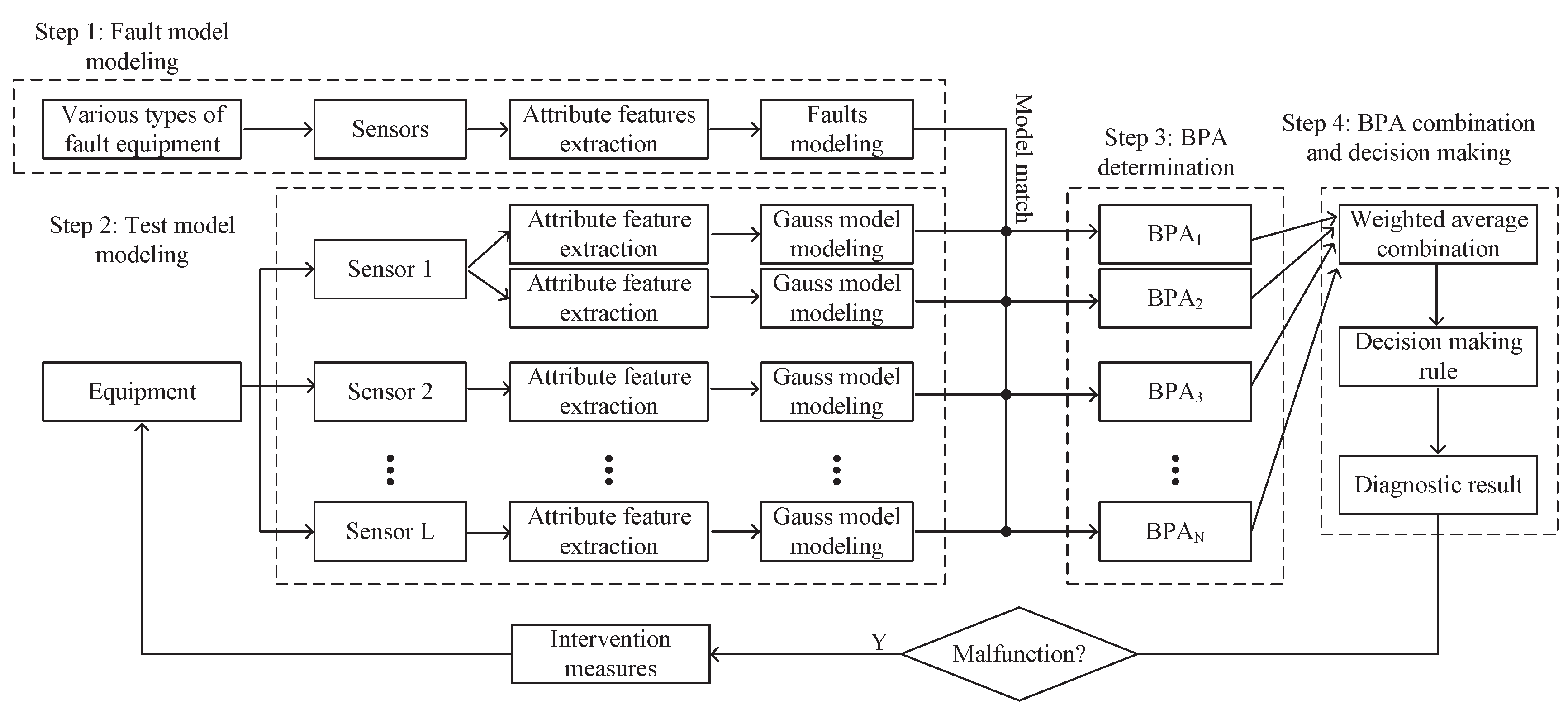
Figure 2.
Graphical introduction of intersection area if . (a), (b), (c) shows the , , , respectively.
Figure 2.
Graphical introduction of intersection area if . (a), (b), (c) shows the , , , respectively.

Figure 3.
Training models and test models of four attributes. (a), (b), (c), (d) depicts training models and test model under attribute , respectively.
Figure 3.
Training models and test models of four attributes. (a), (b), (c), (d) depicts training models and test model under attribute , respectively.
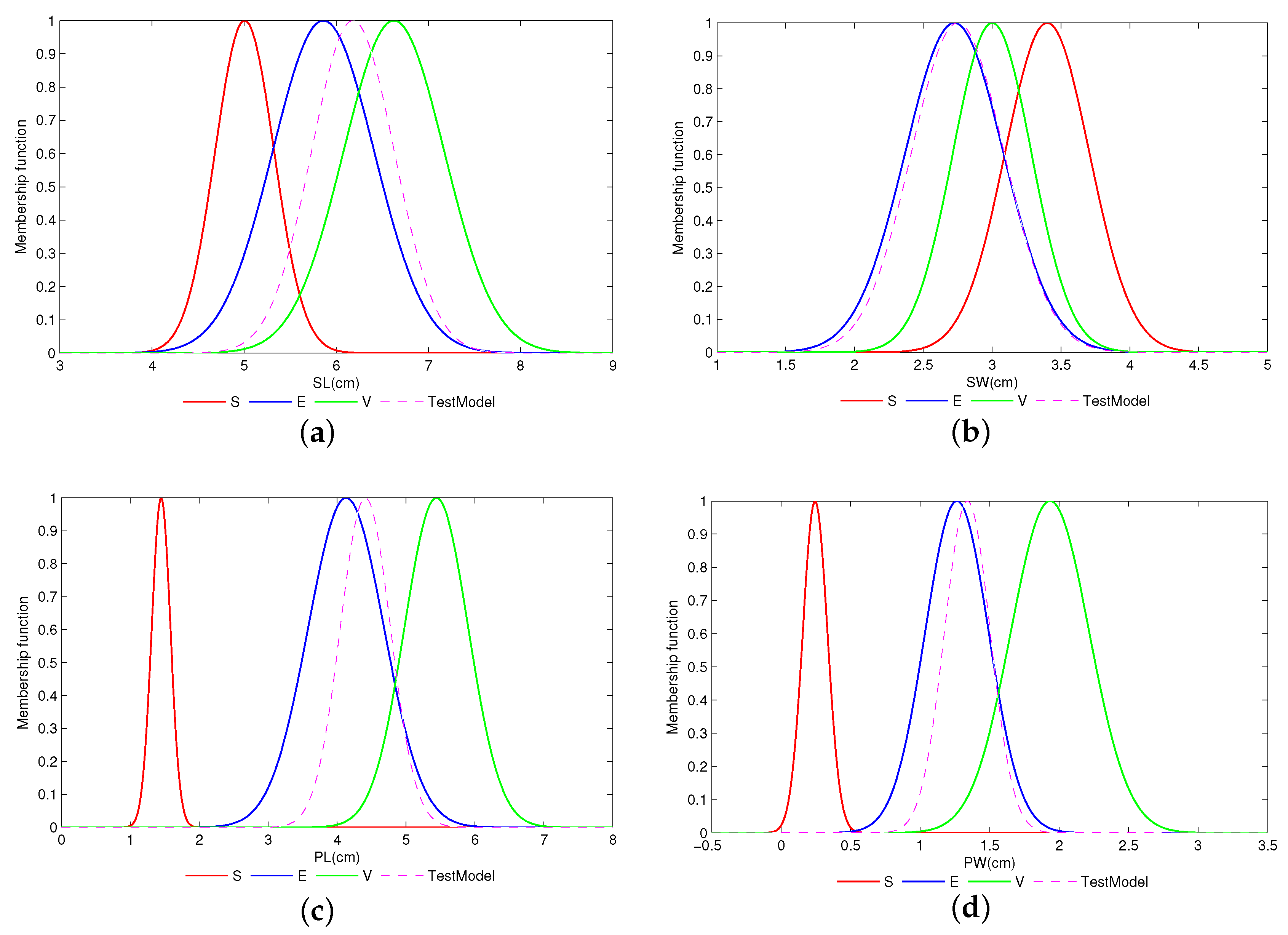
Figure 4.
Generated fault models (i = 1, 2, 3) and test model . (a) shows the generated fault models (i = 1, 2, 3); (b) shows the generated test model .
Figure 4.
Generated fault models (i = 1, 2, 3) and test model . (a) shows the generated fault models (i = 1, 2, 3); (b) shows the generated test model .
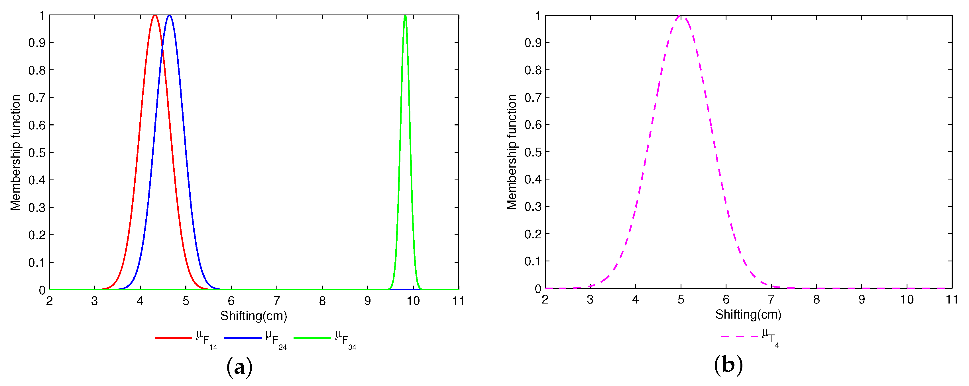
Figure 5.
Intersection area of fault models and test model under feature 4 (). (a), (b), (c) shows the , , , respectively.
Figure 5.
Intersection area of fault models and test model under feature 4 (). (a), (b), (c) shows the , , , respectively.


| Category | ||||
|---|---|---|---|---|
| S | (5.0050, 0.3203) | (3.4000, 0.3061) | (1.4450, 0.1356) | (0.2450, 0.0887) |
| E | (5.8600, 0.5510) | (2.7250, 0.3567) | (4.1300, 0.5497) | (1.2650, 0.2277) |
| V | (6.6250, 0.5466) | (3.0000, 0.2847) | (5.4400, 0.4627) | (1.9350, 0.2815) |
| TestModel | (6.1800, 0.4492) | (2.7500, 0.3375) | (4.4100, 0.3635) | (1.3400, 0.1647) |
| Category | |||||||
|---|---|---|---|---|---|---|---|
| 0.1086 | 0.8324 | 0.7254 | 0.1086 | 0.0595 | 0.5934 | 0.0595 | |
| 0.2982 | 0.9919 | 0.6336 | 0.2974 | 0.2980 | 0.6289 | 0.2974 | |
| 2 × | 0.9196 | 0.2416 | 1.9 × | 2 × | 0.2385 | 2 × | |
| 1.2 × | 0.9660 | 0.2470 | 1.1 × | 5.5 × | 0.2471 | 5.5 × |
: sepal length; : sepal width; : petal length; : petal width.
| Category | |||||||
|---|---|---|---|---|---|---|---|
| 0.0437 | 0.3346 | 0.2916 | 0.0437 | 0.0239 | 0.2385 | 0.0239 | |
| 0.0865 | 0.2879 | 0.1839 | 0.0863 | 0.0865 | 0.1825 | 0.0863 | |
| 1.4 × | 0.6570 | 0.1726 | 1.3 × | 1.4 × | 0.1704 | 1.4 × | |
| 8.2 × | 0.6616 | 0.1692 | 8.2 × | 3.8 × | 0.1692 | 3.8 × | |
| Final BPA | 4.9 × | 0.8798 | 0.1130 | 3.3 × | 2.2 × | 0.0066 | 1.5 × |
| Category | Test Times | Identification Accuracy |
|---|---|---|
| S | 10,000 | |
| E | 10,000 | |
| V | 10,000 |
| Category of Models | Mean Value | Standard Deviation |
|---|---|---|
| 4.3241 | 0.3240 | |
| 4.6414 | 0.3087 | |
| 9.8220 | 0.1010 | |
| 5.0105 | 0.6455 |
| Category | |||||||
|---|---|---|---|---|---|---|---|
| 0.0773 | 0.8452 | 0 | 0.0775 | 0 | 0 | 0 | |
| 0 | 0.4052 | 0.2974 | 0 | 0 | 0.2974 | 0 | |
| 0 | 0.9995 | 0.0002 | 0 | 0 | 0.0003 | 0 | |
| Final BPA | 0.0020 | 0.9973 | 0.00056 | 0.0001 | 0 | 0.00004 | 0 |
| Case | Real Category | Combined BPA | Diagnostic Category |
|---|---|---|---|
| 1 | |||
| 2 | |||
| 3 | |||
| 4 | |||
| 5 |
© 2017 by the authors. Licensee MDPI, Basel, Switzerland. This article is an open access article distributed under the terms and conditions of the Creative Commons Attribution (CC BY) license ( http://creativecommons.org/licenses/by/4.0/).
Share and Cite
MDPI and ACS Style
Jiang, W.; Hu, W.; Xie, C. A New Engine Fault Diagnosis Method Based on Multi-Sensor Data Fusion. Appl. Sci. 2017, 7, 280. https://doi.org/10.3390/app7030280
AMA Style
Jiang W, Hu W, Xie C. A New Engine Fault Diagnosis Method Based on Multi-Sensor Data Fusion. Applied Sciences. 2017; 7(3):280. https://doi.org/10.3390/app7030280
Chicago/Turabian StyleJiang, Wen, Weiwei Hu, and Chunhe Xie. 2017. "A New Engine Fault Diagnosis Method Based on Multi-Sensor Data Fusion" Applied Sciences 7, no. 3: 280. https://doi.org/10.3390/app7030280
Note that from the first issue of 2016, this journal uses article numbers instead of page numbers. See further details here.