Development of a Preliminary Design Method for Subsonic Splittered Blades in Highly Loaded Axial-Flow Compressors

Abstract

This paper presents a model for predicting the reference minimum-loss incidence and deviation angles of a blade arrangement with splitter vanes, which is probably a solution for future ultra-highly loaded axial compressor designs. The motivation of the modeling is to guide the blading design in splittered compressor design processes where the additional splitter vanes must be specially considered. The development of the model is based on a blade performance database from systematic numerical simulations. Basic correlations of the model are firstly proposed, which consider dominant blade geometry parameters related to blade loading, including camber angle and solidity. Secondly, geometric and aerodynamic corrections about orientation parameter, blade maximum thickness, inlet Mach number, and three-dimensional (3D) effects are empirically incorporated into the basic correlations. Eventually, a subsonic 3D splittered rotor is designed using the correlations coupled with the corrections obtained from the validation of the model. The results indicate that the model is able to achieve a good agreement within an error band of ±1.0° for the predictions of both reference minimum-loss incidence and deviation angles, and the rotor designed using the model accomplishes the desired work input and flow deflection.

1. Introduction

An advantageous compressor design in terms of compactness, weight, and cost is needed for gas turbine engines. This can be accomplished by directly reducing the number of stages required to provide a desired pressure ratio in a multistage compressor. Aerodynamically, the reduction of stages will certainly need to increase the total enthalpy rise, i.e., loading level, of each stage. A highly loaded compressor usually means a high relative Mach number or/and high blade aerodynamic diffusion to achieve this high total enthalpy rise across each stage, which results in a high work coefficient (usually more than 0.5), as discussed by Dickens et al. [1]. In order to achieve this goal, increasing the blade speed (hence higher relative inflow Mach number for a rotor) or/and flow deflection (hence higher blade surface diffusion for a rotor or stator) can be employed. These methods usually cause increased deviation angles and aerodynamic losses under much stronger adverse pressure gradient for the highly loaded blades so that the blade performance tends to deteriorate.

Considering the successful applications of splitter vanes (SVs) in centrifugal compressors, the cascade arrangement with SVs has been used in supersonic and subsonic axial flow compressors as a flow control method to reduce the deviation angles and losses under the high loading condition by Wennerstrom et al. [2], Tzuoo et al. [3], Chen [4], and Hobson et al. [5]. The concept is to incorporate a SV in the rear blade passage, thereby increasing solidity locally without substantially increasing throat blockage, which is expected to strengthen flow deflection but reduce the local flow diffusion level on the suction surface of principal blades (PBs). In a subsonic axial compressor cascade investigated by Li et al. [6], for instance, splittered blades have shown potential to achieve higher pressure ratio, efficiency, and mass flow compared to conventional blade at the studied subsonic condition.

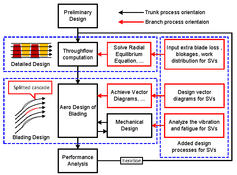
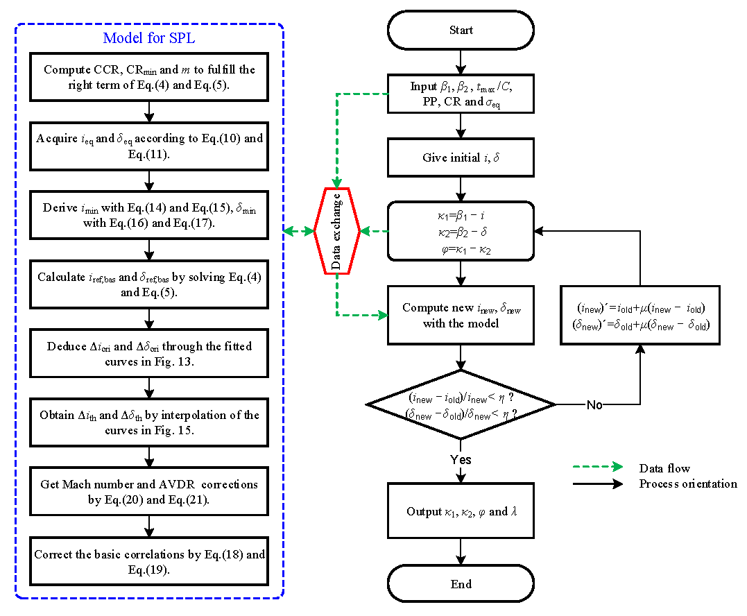
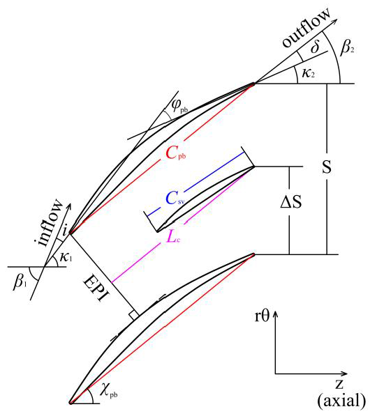
However, because of the geometric difference between the PB and the SV, the design procedures of a splittered compressor should be different to those of a conventional one, as shown in Figure 1. Obviously, the incorporation of the extra SVs makes the design freedoms of blade geometry at least double compared to conventional blades, which on the one hand brings extra possibilities for performance improvement, but on the other hand makes the design process much more complicated. Nevertheless, it is the same with the design of conventional blades: blading design also plays a critical role in the design of high-performance splittered compressors. One of the important goals in blading design is to achieve desired velocity triangles (vector diagrams) derived from throughflow computations at different spanwise locations. It is only when the desired velocity triangles are appropriately satisfied that a given work input (for rotors), pressure rise, and flow deflection (for stators) can be achieved.

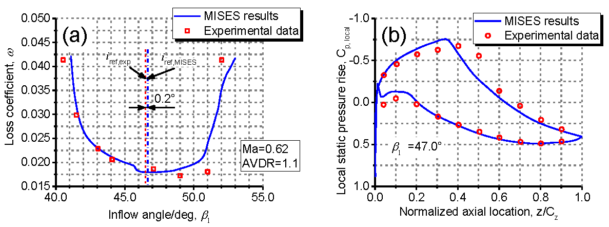
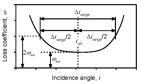
To do that, a model for predicting the reference minimum-loss incidence and deviation angles, which are usually selected as design goals, is required to obtain some blade profile parameters, such as camber angle and stagger angle, for the blading design. The reference minimum-loss incidence and deviation angles, which were proposed by Lieblein [7], are both usually defined at the middle of incidence range between two points corresponding to twice the minimum loss at the loss-to-incidence-angle characteristic line of a certain blade, as shown in Figure 2. Unfortunately, according to the authors’ knowledge, few studies on the topic have been openly published for the blades with SVs, except for the work conducted by Tzuoo et al. [3]. However, Tzuoo et al. only considered the variation of deviation angles with the solidity and camber of SVs.

Hence, in the present work, the minimum-loss incidence and deviation angles in axial-flow splittered compressors will be modeled as the additional consideration of SVs. The modeling is based on a database established using the widely applied and validated quasi-three dimensional codes MISES [8]. Moreover, in order to consider the effects of inflow angle, inlet Mach number, camber angle, solidity, blade maximum thickness, and even three-dimensional flow in blade passage (i.e., axial velocity density ratio, AVDR), the model will be corrected using the methods employed in some classical models for conventional blade profiles [7,9,10,11].

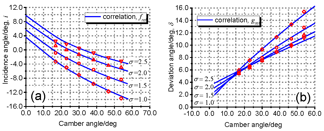
In order to establish the database with representative blades, which should be designed with geometries in reasonable ranges, three highly loaded blades were first investigated by varying circumferential position and local incidence of SVs. Then, based on the optimal geometry arrangement, the profile performance at full incidence range was computed for two-dimensional (2D) blades of different camber angle, solidity, and chord length of SVs so as to produce a basic database. This basic database contains the basic correlations of reference minimum-loss incidence and deviation angles. Subsequently, additional analyses of the corrections for orientation parameter, maximum thickness-chord ratio, inlet Mach number, and AVDR were performed to modify the basic correlations. The model was also employed to guide the blade design for a subsonic axial-flow rotor with SVs.

2. Modeling Methodology for Blade Profile with SV

2.1. Geometry Parameters and Aerodynamic Conditions

A representative blade section of the axial flow compressor cascades with SVs used in the study is shown in Figure 3. Both the trailing edge axial position and the blade outlet metal angle of the SVs were set exactly the same as those of PBs. Both the SVs and PBs were generated using circular-arc camber lines with the thickness distribution of the NACA65 profile and the same blade maximum thickness-chord ratio.

In order to model the flow in blades with SVs in the present study, the basic correlations referred from some classical models were established at first. The basic correlations were derived based on a reference blade family. The reference blade family was characterized by an identical blade inlet metal angle of 63° and maximum thickness-chord ratio of 6.0%. Blade inlet metal angle, instead of stagger angle or inflow angle used as blade orientation by Lieblein [7], was treated as the orientation parameter in the study. On the other hand, the reference aerodynamics conditions were maintained with an inflow Mach number of 0.1, an axial velocity density ratio (AVDR) of 1.0, and a Reynolds number of 1.0 × 10⁶. All off-reference conditions have been corrected under the same Reynolds number so as to extend the application of the model.

In the study, two new geometry parameters are defined for splittered cascades. The geometry definitions of the two parameters are shown in Figure 3. One is the effective passage inlet (EPI), which is a line from the leading edge of PBs perpendicular to the suction surface of adjacent PBs. The other one is critical length L_c, which is a line parallel to the chordwise direction of PBs from the trailing edge of SVs to the EPI. The critical length ratio (CLR) is the ratio of the critical length L_c to the chord of PBs. According to the research by Li et al. [6], the effects of a SV on upstream flow field become more significant when the leading edge of a SV is upstream of the EPI, or when the chord length of a SV is longer than L_c. Therefore, the two geometry parameters are expected to act as important factors of the model.

2.2. Ranges of Geometry Parameters

In order to establish the CFD database for the modeling analyses of the basic correlations, analyzed splittered cascades were first chosen with the variation of different geometry parameters and the chord length of SVs in a representative range as listed in

Table 1. Ranges of different parameters for the basic correlations.

Parameters	Splittered Cascades	Conventional Cascades
inlet metal angle, κ1 (°)	~63	~63
camber angle, φpb (°)	16.8–65.2	16.8–71.5
stagger angle, χpb (°)	54.5–36.5	54.5–36.5
equivalent solidity (ES), σeq = (Cpb + Csv)/S	1.21–2.04	0.95–2.55
diffusion factor (DF)	0.26–0.65	0.28–0.67
chord ratio, CR = Csv/Cpb	0.25–0.92	—
percent pitch (PP)	0.5	—

. For the comparison analyses of the results for splittered cascades with the conventional cascades, systematic calculations of conventional cascades were simultaneously conducted within the ranges of different parameter groups, which are also listed in Table 1.

It is necessary to explain that the diffusion factor (DF) defined for splittered cascades is modified by replacing the solidity in traditional definition with the equivalent solidity (ES) as formulated by Equation (1):

$$\mathrm{DF}=1-\frac{\cos {\beta }_1}{\cos {\beta }_2}+\frac{\cos {\beta }_1}{2{\sigma }_{\mathrm{eq}}}\left(\tan {\beta }_1-\tan {\beta }_2\right).$$

(1)

DF has been widely applied in compressor aerodynamics as a measure of blade loading. It describes the magnitude of blade suction surface flow diffusion. A value of 0.6 is regarded as the load limit of conventional blades according to Lieblein [7]. It can be seen in Table 1 that the variation of DF has covered a significantly wide loading range for both splittered cascades and conventional cascades.

2.3. Systematic Variation of Chord Ratio

In a specific combination of different geometry parameters, the chord ratio (CR) was systematically increased while the other parameters were kept as constant values in order to observe the effects of CR on the reference minimum-loss incidence and deviation angles. The dynamic growth of CR is sketched in Figure 4 where the chord of PBs is kept constant and the pitch is increased to maintain the fixed value of ES. When CR exactly equals to CLR, i.e., when C_sv = L_c, a critical chord ratio (CCR) can be defined as follows:

$$\mathrm{CCR}=\frac{{\sigma }_{\mathrm{eq}}-\left(1-\mathrm{PP}\right)\sin {\chi }_{\mathrm{pb}}}{{\sigma }_{\mathrm{eq}}+\left(1-\mathrm{PP}\right)\sin {\chi }_{\mathrm{pb}}}.$$

(2)

This expression can be readily derived by introducing the definition of ES into that of CLR to eliminate the term of pitch-to-chord ratio of PBs. The corresponding chord of SVs and solidity of PBs are defined as critical chord C_sv,cr and critical solidity (CS) σ_cs, respectively. CCR could be an important factor of the basic correlations.

2.4. Numerical Method

A quasi-three dimensional code MISES by Drela et al. [8] was utilized in order to evaluate the blade profile performances. The code is functional in both direct and inverse design of compressor blade sections. Considering its advantages in terms of simplification and time saving, MISES has been widely validated and used for both scientific studies and industry applications [1,9,12,13,14].

The calculated flow domain in MISES is divided into an inviscid outer flow region and a boundary layer region, which are iteratively solved using different equations. The inviscid flow is computed by the Euler equations, and boundary layer computations are based on the classic Kármán integral momentum equation and the integral kinetic energy equation. The grid points are established by using an elliptic grid generator in the domain of inviscid flow, determining the streamlines and quasi-normal lines. The flow field is discretized by a finite volume method so that the Newton–Raphson solver can be used to simultaneously solve the non-linear equations of the two zones. The edge velocity and density are first derived from the equations of inviscid outer flow to promote the integral boundary solutions for the displacement thickness, which corrects the edge of inviscid outer flow in turn. The iteration is performed until the convergence criterion is reached. The work of Youngren [15] can be referred to for more details about the numerical formulation.

In order to validate the code, Figure 5 gives a comparison between MISES calculation results and experimental data for a hub section of the first stage in an industrial compressor inversely designed by Steinert et al. [16]. It can be seen in Figure 5a that MISES results are in good agreement with the experimental data as the difference of about 0.2° in reference minimum-loss definition is acceptable in this study. Figure 5b shows the comparison of blade surface pressure distribution at the inflow angle of 47.0°. It is indicated that the MISES-predicted surface pressure distribution is basically in agreement with the experimental results despite a slight difference of suction peak location.

Table 2. Performances from experiments and MISES computations.

Parameters	Ma	β1	β2	Ps2/Ps1	ω
Experiments	0.62	47.0	20.2	1.1221	0.0186
MISES computations	0.62	47.0	20.9	1.1221	0.0182

shows the performance results from experiments and MISES computations at inflow angle of 47.0°. It is indicated that the outflow angle, the pressure ratio, and the total pressure loss coefficients used for performance analyses are in excellent agreement. The validation indicates that the code can accurately predict not only reference minimum-loss definition but also surface pressure distribution and profile performances required for analyses and modeling in the present study.

3. Effects of Incidence Angle and Circumferential Location of Splitter Vane

In order to establish the basic correlations mentioned above at first, a database for representative splittered cascades should be created by using CFD method. Based on the following analyses, it can be found that the appropriate design incidence angle and circumferential location of SVs should be set for the analyzed cases.

3.1. Studied Cases

Three cases with different blade loading and various CR were constructed for analyses of effects of incidence angle and circumferential location of splitter vane. The geometry parameters of the three cases are shown in

Table 3. Geometry parameters of three splittered cascades for performance sensitivity analyses.

Parameters	Case_1	Case_2	Case_3
camber angle, φpb (°)	46.7	46.7	53.8
equivalent solidity (ES), σeq	2.04	2.04	1.59
principal blade solidity, σpb	1.39	1.21	1.08
chord ratio (CR)	0.47	0.68	0.47
diffusion factor (DF), PP = 0.5	0.51	0.55	0.62
percent pitch (PP)	0.22–0.83

.

Two incidence design rules were successively used to design the SVs of all three cases. One was that SVs were simply given the same camber lines as those of PBs at the same axial position according to Tzuoo [3] and Wennerstrom et al. [17]. This resulted in an automatic design of incidence for SVs by subtracting the blade inlet metal angle from the local inflow angle. The other one was that the inlet metal angle was properly set for the leading edge of SVs to adapt to the local inflow angle so that the stagnation point was exactly located at the intersection of the leading edge and the camber line. The setting was considered to form an “impact-free entry” condition so as to smooth the pressure distribution on both suction surface (SS) and pressure surface (PS) of SVs according to Cumpsty [11]. The smooth pressure distribution usually results in lower loss and a higher pressure ratio. The three cases using the former incidence rule for SVs have been named original designs, and the latter are “impact-free entry” designs.

In addition, the percent pitch (PP) was varied to examine the effects of circumferential position of SVs on profile performances for all of the three cases designed by different incidence rules.

3.2. Blade Performance with Different Incidence Angles and Circumferential Locations

Figure 6 plots the total pressure loss and pressure rise on the design condition for both the original designs and the “impact-free entry” designs. It can be seen that the two incidence rules have consistent effects on total pressure loss for the cascades with different blade loading level. For Cases 1 and 2 with comparably lower loading, it is showed that the “impact-free entry” designs have benefits somewhat compared to the original designs. In addition, significant gains can be attained for Case 3 with comparably higher blade loading, especially at a large range of PP. The overall static pressure rise is essentially insensitive to the incidence rules. On the other hand, PP itself has a significant influence on blade pressure rise and loss. It is indicated that the responses of the “impact-free entry” designs to PP remain similar as those of the original designs. For Cases 1 and 2 with comparably lower loading, it is illustrated that they have the smallest loss at PP = 0.5. For Case 3, larger PP is, surprisingly, associated with lower loss. As for the static pressure rise, all the three cases show consistently a peak pressure rise at about PP = 0.5.

Figure 7 presents the blade surface pressure distributions at different PP for Case 2. For the typical case, it shows that all “impact-free entry” designs eliminate the strong leading-edge acceleration on SS or PS due to the improper selection of incidence angles for SVs. This explains why the “impact-free entry” designs show lower loss in Figure 6.

On the other hand, it is indicated that the pressure distribution is considerably influenced by PP. At PP = 0.5 in Figure 7b, the principal blade and splitter vane have similar blade surface pressure distribution, resulting in a suitable balance in loading between the two blades. This favorable pressure distribution contributes to the highest static pressure rise in Figure 6. As SVs are located near PBs, the interaction of SVs and PBs tends to be stronger. At PP = 0.83 in Figure 7a, the acceleration of the SS of SVs significantly decreases the pressure of the PS of PBs so that the rear part of PBs is completely unloaded. Therefore, the overall static pressure rise apparently decreases, as shown in Figure 6. At PP = 0.22 in Figure 7c, the peak on PS of the SVs is higher because of the acceleration at the front part of PS of SVs so that the load of SVs is decreased. That is why lower PP decreases the overall static pressure rise.

3.3. Determination of Incidence Angle and Circumferential Location for SVs

In summary, “impact-free entry” design and PP = 0.5 should be selected for the model, which are supposed to achieve the maximum loading and reduce the loss as much as possible. Equation (3) gives the formulation of local incidence angles for SVs to satisfy the “impact-free entry” design when the CR is systematically increased. The incidence angle of SVs gradually transforms into the reference minimum-loss incidence angle of equivalent conventional blades in a polynomial manner when C_sv is longer than C_sv,cr from the value of 0:

$$i_{\mathrm{sv}}=\{\begin{array}{lll}{i}_{\mathrm{eq}}{\left(\frac{C_{\mathrm{sv}}-C_{\mathrm{sv},\mathrm{cr}}}{C_{\mathrm{pb}}-C_{\mathrm{sv},\mathrm{cr}}}\right)}^2& ,& C_{\mathrm{sv}}\ge C_{\mathrm{sv},\mathrm{cr}}\\ 0& ,& C_{\mathrm{sv}}<C_{\mathrm{sv},\mathrm{cr}}\end{array}.$$

(3)

4. Basic Correlations for Reference Conditions

Based on the selected “impact-free entry” incidence rule and PP = 0.5 for SVs, the blade performance computations were carried out for different parameter combinations with the systematic variations of CR. The results in reference conditions are used for the basic correlations in the following modeling.

4.1. Variation Profiles with CR

Figure 8 presents a typical instance of profiles of the reference minimum-loss incidence and deviation angles with varied CR for a certain parameter combination. It is shown that there is a minimum value for both angles. In addition, when CR is between zero and unit, both angles are lower than those of conventional cascades for which CR equals zero or unit. Any other combinations of different geometry parameters have similar profiles.

To model the profiles discussed above, a profile function is employed, which is formulated algebraically by Equations (4) and (5).

$$\frac{i_{\mathrm{bas}}-i_{\min }}{i_{\mathrm{eq}}-i_{\min }}={\left[1-\exp \left(n{C}^m\right)\right]}_i$$

(4)

$$\frac{{\delta }_{\mathrm{bas}}-{\delta }_{\min }}{{\delta }_{\mathrm{eq}}-{\delta }_{\min }}={\left[1-\exp \left(n{C}^m\right)\right]}_{\delta }.$$

(5)

For the left terms, both incidence and deviation angles are normalized by a non-dimensional parameter group composed of the corresponding minimum and equivalent values of the incidence and deviation angles. The index “bas” represents the basic correlations for the reference minimum-loss angles.

The right terms primarily involve the CR and CR_min (denoting the CR at the minimum of incidence or deviation angles) as the basic components of C and m shown in Equations (6) and (7):

$$C=\frac{\mathrm{CR}-{\mathrm{CR}}_{\min }}{\epsilon \left(\mathrm{CR}-{\mathrm{CR}}_{\min }\right)-{\mathrm{CR}}_{\min }}$$

(6)

$$m=m_{\mathrm{L}}+\left(m_{\mathrm{R}}-m_{\mathrm{L}}\right)\epsilon \left(\mathrm{CR}-{\mathrm{CR}}_{\min }\right),$$

(7)

where the expression ε(x) is a step function, as expressed in Equation (8). Through the analyses based on the database, CR_min can be approximately formulated in a linear manner with CCR and camber, which is shown in Equation (9):

$$\epsilon \left(x\right)=\{\begin{array}{ll}\mathrm{0,}& x\le 0\\ \mathrm{1,}& x>0\end{array}$$

(8)

$${\mathrm{CR}}_{\min }=\mathrm{CCR}+a\phi +b.$$

(9)

All constant coefficients used in the basic correlations are given in

Table 4. Constant coefficients for the basic correlations.

Coefficients	n	mL	mR	a	b	kcs	keq	kδ
for i	−6.38	2.0	2.67	−4.89 × 10−3	9.33 × 10−2	0.5	0.5	1.1
for δ	−3.36	4.0	2.96	−5.32 × 10−4	−1.92 × 10−1

. The coefficients are attained by adequately fitting the basic CFD data so as to reduce the correlation errors.

4.2. Equivalent Values of Incidence and Deviation Angles

The variables of i_eq and δ_eq herein can be gained by a typical correlation methodology developed by Lieblein [7] for conventional blades, which has been extensively employed by Banjac et al. [9], McGlumphy [18], and Zachos et al. [19]. The method can be expressed implicitly by Equations (10) and (11):

$$i_{\mathrm{eq}}=f_{\mathrm{ref}}\left(K_{i\mathrm{mod}}\phi ,{\kappa }_1+i_{\mathrm{eq}},{\sigma }_{\mathrm{eq}},t_{\max }/C\right)$$

(10)

$${\delta }_{\mathrm{eq}}=g_{\mathrm{ref}}\left(K_{\delta \mathrm{mod}}\phi ,{\kappa }_1,{\sigma }_{\mathrm{eq}},t_{\max }/C\right),$$

(11)

where extra correction functions, namely K_{i mod} and K_{δ mod}, are added to the correlations to adapt to the NACA 65 profile with a circular-arc camber line. In addition, the orientation parameter is changed to blade inlet metal angles from (the original) inflow angles.

The correction functions K_{i mod} and K_{δ mod} have the same format with three empirical constant coefficients, as expressed in Equations (12) and (13), which mainly consider the effects of solidity on the basic correlations. The constant coefficients are tabulated in

Table 5. Constant coefficients for the correction functions of equivalent conventional blades.

Coefficients	μ1	μ2	μ3
for i	0.12419	0.96242	1.25391
for δ	−0.43210	−0.58577	1.18477

.

$${\mathrm{K}}_{i\mathrm{mod}}={\left({\mu }_1\exp \left(\sigma /{\mu }_2\right)+{\mu }_3\right)}_i$$

(12)

$${\mathrm{K}}_{\delta \mathrm{mod}}={\left({\mu }_1\exp \left(\sigma /{\mu }_2\right)+{\mu }_3\right)}_{\delta }.$$

(13)

To validate the conventional blade correlations, Figure 9 gives the comparisons of reference minimum-loss incidence and deviation angles with CFD database. It can be seen that the correlation curves are in excellent agreement with the symbols, which allows for accurate prediction of i_eq and δ_eq for the basic correlations.

4.3. Minimum Values of Incidence and Deviation Angles

The variable i_min is also intended to be modeled by the correlation of conventional blades f_ref. As shown in Figure 10a, the variable i_min can be obtained from the correlation of conventional blades f_ref, which has a special solidity, σ_se. Therefore, the variable i_min can be expressed as in Equation (14). It is found that the special solidity can be expressed linearly with σ_cs and σ_eq, as shown in Equation (15), where the constant coefficients k_cs and k_eq have been previously listed in Table 4. The special solidity can be graphically derived through Figure 10a. It is necessary to note that the values of the geometry parameters substituted into the conventional blade correlation f_ref, including the camber angle, inlet metal angle and maximum thickness-chord ratio, are the same as those of the corresponding PBs. The predictions of the minimum incidence values based on the effects of solidity of PBs are in good agreement with the CFD database, as presented in Figure 10b.

$$i_{\min }=f_{\mathrm{ref}}\left(K_{i\mathrm{mod}}\phi ,{\kappa }_1+i_{\min },{\sigma }_{\mathrm{se}},t_{\max }/C\right)$$

(14)

$${\sigma }_{\mathrm{se}}=k_{\mathrm{cs}}{\sigma }_{\mathrm{cs}}+k_{\mathrm{eq}}{\sigma }_{\mathrm{eq}}.$$

(15)

Similarly, the variable δ_min can be derived by a liner combination of δ_cs and δ_eq, as given in Equation (16). The variable δ_cs equals the deviation angle of conventional blades but with the solidity replaced by σ_cs, as shown in Equation (17):

$${\delta }_{\min }={\delta }_{\mathrm{eq}}-k_{\delta }\left({\delta }_{\mathrm{cs}}-{\delta }_{\mathrm{eq}}\right)$$

(16)

$${\delta }_{\mathrm{cs}}=g_{\mathrm{ref}}\left(K_{\delta \mathrm{mod}}\phi ,{\kappa }_1,{\sigma }_{\mathrm{cs}},t_{\max }/C\right).$$

(17)

Figure 11a illustrates the graphical derivation. Figure 11b gives a comparison between the correlation values and CFD database, which also shows good agreement.

4.4. Comparisons of the Model Predicted and CFD Calculated Results

Figure 12 shows the comparisons between the results obtained based on basic correlations and CFD calculations. The results indicate that the correlations of both reference minimum-loss incidence and deviation angles essentially match the database in a certain error band. For reference minimum-loss incidence correlation, the error band is limited within ±1°. For reference minimum-loss deviation correlation, the error band is not beyond ±0.5°. The accuracy of prediction for the reference minimum-loss incidence and deviation angles enhances the confidence of further expanding the feasibility of the model for off-reference conditions.

5. Corrections for Off-Reference Conditions

The aforementioned basic correlations have considered the effects of camber angle and solidity for the fixed orientation parameter, maximum thickness-chord ratio, inlet Mach number, and AVDR, which are regarded as the reference conditions. Therefore, it is necessary to correct the correlations with off-reference conditions so as to apply the model under practical compressor circumstances. Based on the basic correlations, the reference minimum-loss incidence and deviation angles can be modified with additional corrections from different factors, as shown in Equations (18) and (19):

$$i_{\mathrm{mod}}=i_{\mathrm{bas}}+\Delta i_{\mathrm{ori}}+\Delta i_{\mathrm{th}}+\Delta i_{\mathrm{Ma}}+\Delta i_{3\mathrm{D}}$$

(18)

$${\delta }_{\mathrm{mod}}={\delta }_{\mathrm{bas}}+\Delta {\delta }_{\mathrm{ori}}+\Delta {\delta }_{\mathrm{th}}+\Delta {\delta }_{\mathrm{Ma}}+\Delta {\delta }_{3\mathrm{D}},$$

(19)

where the indexes ori, th, Ma, and 3D represent the corrections for orientation parameter, maximum thickness, Mach number, and AVDR, respectively.

5.1. Correction of Orientation Parameter

Some extra CFD calculations were carried out to correct the basic correlations for orientation parameter. The ranges of the different parameters used for the correction are listed in

Table 6. Parameter ranges for the correction of orientation parameter.

Parameters	Ranges
inlet metal angle, κ1 (°)	43, 53, 73
camber angle, φpb (°)	30, 50
equivalent solidity, σeq	1.4, 1.8
chord ratio(CR)	0.45, 0.65, 0.85

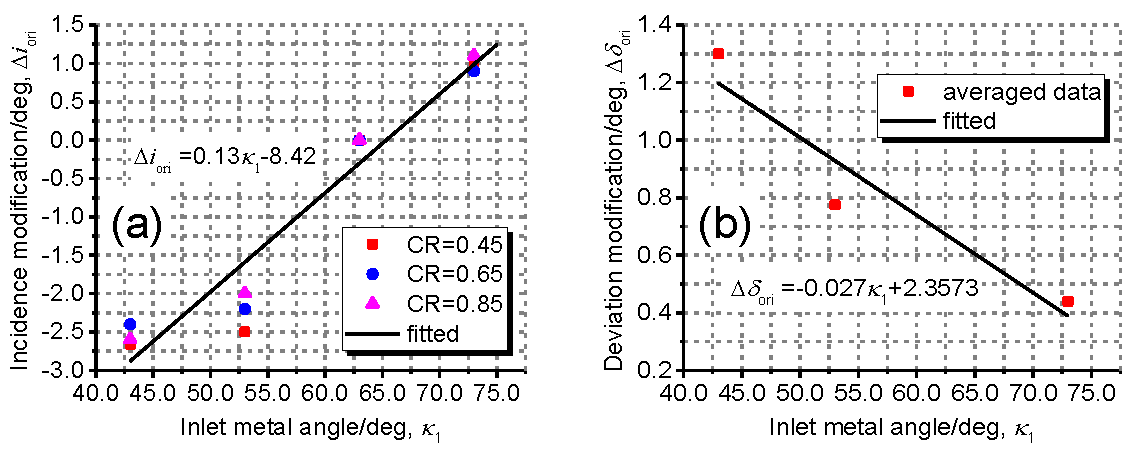
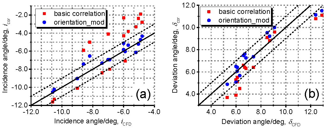
, which synthetically include the parameters of inlet metal angle, camber angle, solidity, and CR. Figure 13 presents the correction curves with blade inlet metal angle as the only independent variable. It was found that all the other geometry parameters have a slight influence on the correction curves based on the results of the database. Through the averaged modifications, it is plausible that the correction curves can be treated as approximately linear curves.

Figure 14 compares the results obtained by using basic correlations and the modified correlations. It is shown that the modified correlations have higher accuracy to match the CFD results compared to basic correlations. In addition, the scatter points almost concentrate within a certain error band of ±1° for the predicted results from the modified incidence and deviation correlations.

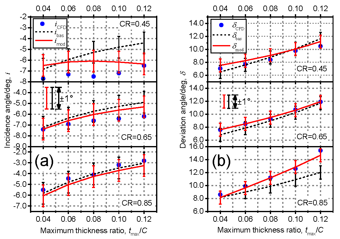
5.2. Correction of Maximum Thickness-Chord Ratio

The correction of the maximum thickness-chord ratio is more complicated than that of the orientation parameter because of the coupled effects of the maximum thickness and the chord of SVs on the blade passage throat. In view of this fact, it is believed that the CR and the maximum thickness-chord ratio are both supposed to be elementary factors in the correction. Therefore, a series of CFD calculations with CR from 0.45 to 0.85 and maximum thickness-chord ratio from 0.04 to 0.12, which are typical values for the design of blades with SVs, were carried out for the correction of the maximum thickness-chord ratio.

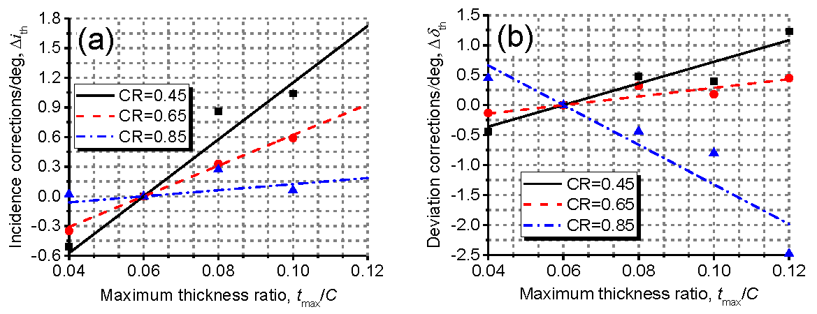
Figure 15 gives the correction curves as a function of the maximum thickness-chord ratio and the CR, linearly fitted using the CFD calculation results. The correction curves match the scatter CFD results well, with a slight error of less than 0.5°.

Figure 16 shows the comparisons between CFD results and the results obtained by using the modified basic correlations combined with the corrections of both orientation parameter and maximum thickness-chord ratio, where basic correlations without the corrections are also presented for evaluating the effect of the improvement of the corrections. It can be seen that the correlations with corrections perform better to match the CFD results compared to the basic correlations, especially for the incidence angles of CR = 0.45 and the deviation angles of CR = 0.85. Moreover, the correlations coupled with these geometry corrections are able to achieve good agreement with the CFD results within the error band of ±1.0° for both incidence and deviation angles.

5.3. Correction of Mach Number

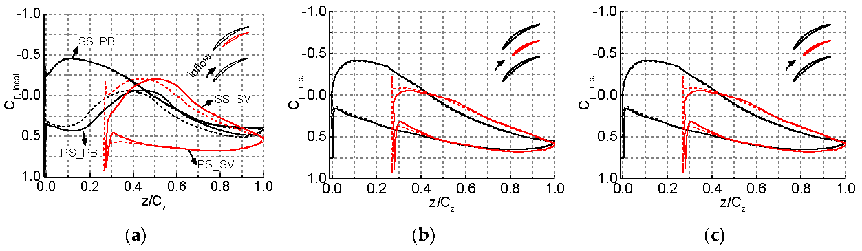
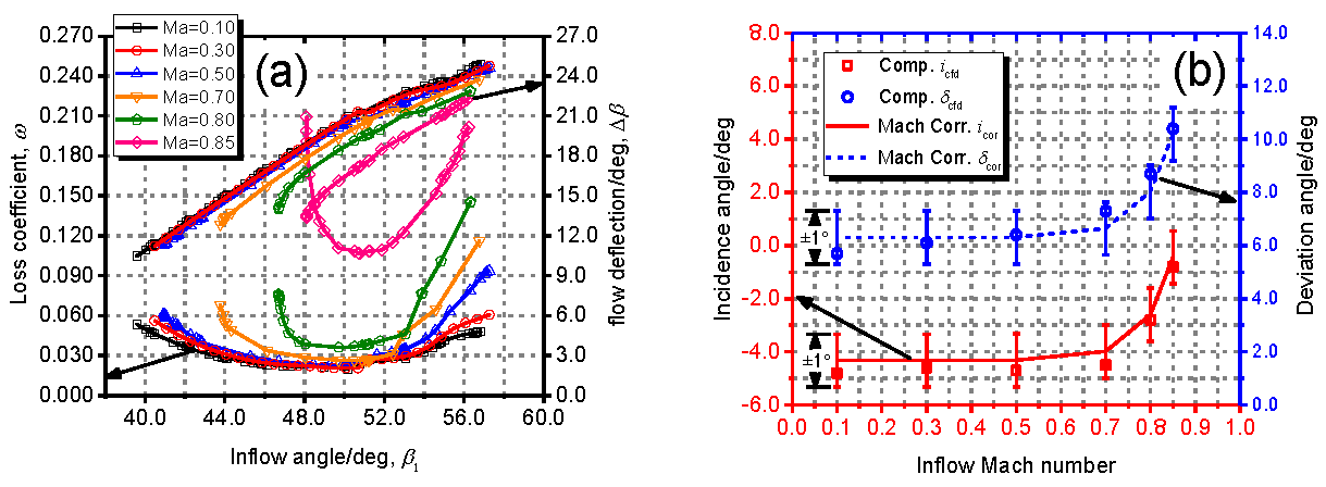
In order to correct the effects of Mach number, a series of CFD computations were performed with the range of subsonic Mach number from 0.10 to 0.85 for blades with various geometry parameters. Figure 17a gives the total pressure loss and deflection angle vs. inflow angle characteristics of a certain splittered cascade with different inlet Mach number. It is indicated that the Mach number does not significantly affect the low loss regions and flow deflection when the Mach number is lower than 0.70. However, as the Mach number exceeds 0.70, the total pressure loss starts to increase, and the flow deflection begins to dramatically drop. It is believed that the supersonic acceleration on the front part of SS of PBs or SVs and the considerable interaction of shock waves with boundary layers are responsible for the performance deterioration.

Figure 17b shows the results of the reference minimum-loss incidence and deviation angles with Mach number for the certain splittered cascade. It can be seen that both of the angles tend to increase with the increased Mach number. As discussed previously, a Mach number of 0.7 is a critical value, above which the incidence and deviation angles increase considerably. The same phenomenon can also be observed for the blades designed with other different geometry parameters. In order to include the effects of the Mach number, the following exponential relationship obtained based on database fitting method could be defined:

$$\Delta i_{\mathrm{Ma}}\approx \Delta {\delta }_{\mathrm{Ma}}=A{e}^{\mathrm{Ma}/B},$$

(20)

where coefficient A has a value of 4.18 × 10⁻⁶ and B has a value of 6.19 × 10⁻². The correction results of Mach number are compared with CFD computation results, as illustrated in Figure 17b, for the certain splittered cascade. Within the error band of ±1.0°, the correlation results agree well with the CFD computation results.

5.4. Correction of Three-Dimensional Flow Effects

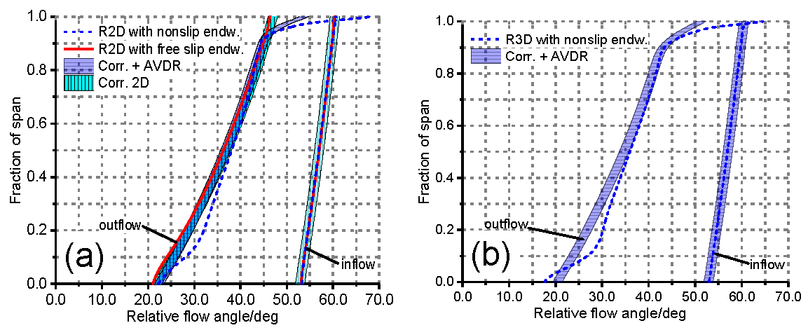
Considering the complexity of 3D flows in axial flow compressors, such as endwall–blade corner separation and blade tip leakage flow (for rotors or cantilevered stators), it is normally difficult to directly consider the induced departures of the 3D flow structures for reference minimum-loss incidence and deviation angles. One of the common methods to include the 3D effects is to correlate the axial velocity density ratio (AVDR) in the model. A well-known correction of AVDR is as follows:

$$\begin{array}{l}\Delta i_{3\mathrm{D}}=-{10.0}^{°}\times \left(1.0-\mathrm{AVDR}\right)\\ \Delta {\delta }_{3\mathrm{D}}={10.0}^{°}\times \left(1.0-\mathrm{AVDR}\right)\end{array}.$$

(21)

The value of AVDR is remarkably affected by the 3D flow blockages, and indirectly reflects the effects of 3D flows on the reference minimum-loss incidence and deviation angles. A comparison between the results from 3D correlation with the AVDR correction and the results from fully 3D numerical simulations will be given in Section 7.

6. Calculation Schemes for the Developed Models

In order to fulfill the blading design process in Figure 1, the model has been coupled with the computation of velocity triangles, which are usually expressed by inflow and outflow angles in subsonic axial flow compressors. The detailed calculation steps of the correlations are presented in the flowchart of Figure 18, where inflow and outflow angles, namely β₁ and β₂, obtained from the throughflow computations, and maximum thickness-chord ratio, percent pitch, chord ratio, and equivalent solidity are the design specifications. The outputs including inlet metal angle, outlet metal angle, camber angle, and stagger angle can be used in the creation of the blade geometry.

7. Design of a Splittered Axial-Flow Rotor and Model Validation

7.1. Design Specifications

An axial-flow rotor with SVs based on the flowpath of the Low-Speed Large-Scale Axial Compressor test platform at Beihang University [20,21] was designed to validate the model. The test platform has been rebuilt for an improved hub-to-casing ratio of 0.75 to simulate the environment of high-pressure core compressors more accurately. The flowpath is in a parallel annulus, which has a constant radius for both the hub and casing. The design parameters for the rotor are shown in

Table 7. Design parameters for a splittered axial-flow rotor.

Parameters	Values
design flow coefficient, ϕ = Vx/Umid	0.65
design work coefficient, ψ = Δh/$U_{\mathrm{mid}}^2$	0.51
mass flow rate (kg/s)	28.2
rotation speed (rev/min)	1100
hub/casing diameter (mm)	750/1000
tip clearance (mm)	1.25
Chord (mm)	114
PB/SV number	24/24
hub/mid/tip ES	1.86/1.59/1.39
aspect ratio	1.1
chord ratio, CR	0.60
percent pitch, PP	0.50
diffusion factor, DFmid	0.45
relative inlet Mach number, Mamid	0.175
Reynolds number, Remid	1.0 × 106

.

In order to exclude the interaction of upstream and downstream blade rows for the model, a single rotor was designed. The meridional stream surface was solved by using a simple radial equilibrium equation with radially uniform work input, resulting in a free vortex design. Accordingly, the relative inflow and outflow angles could be calculated at different spanwise locations from hub to casing, which were the inputs of the blading design process shown in Figure 18. A design line of the relative inflow and outflow angle is given in Figure 19.

Along the design line, the camber angles and stagger angles spanned from hub to casing could be obtained to match the velocity triangles. It should be noted that, if the blade was designed with a constant equivalent solidity of 1.60 from hub to casing, the inflow and outflow angles could be determined based on the results shown in Figure 19. However, in actuality, the equivalent solidity at different spanwise location should be set based on the demand of work input, the limitation of diffusion factor, and the limitation of structural strength. Therefore, the design line shown in Figure 19 only provides initial guesses of the stagger and camber angles, and the final result should be calculated based on the iteration process given in Figure 18. The final blades were stacked along a radial straight line that passed through the gravity center of principal blades at different spanwise locations. This setting could readily satisfy the restriction of structural strength and stress. Figure 20 presents the 3D blades of a splittered axial-flow rotor designed using the developed model.

The rotor designed by the 2D model (R2D as a simplification) is utilized to validate the 2D correlation, and to provide a spanwise distribution of AVDR, which is used to redesign the rotor by using the 3D model. The redesigned rotor is named as R3D for simplification. The redesigned result showed that the flow deflection angles should be increased about two degrees at all spanwise locations to compensate the work deficit due to blade tip clearance leakages and thickened endwall boundary layer.

7.2. 3D Numerical Simulations

Two cases of the R2D were set up for 3D Reynolds-averaged Navier-Stokes computations with an SST turbulence model by using the commercial CFD package CFX. One case was to configure the R2D with a tip clearance of 1.0% span height and the other without tip clearance. The mesh applied for the computation of the R2D with tip clearance is shown in Figure 20. Both the cases had the same O4H topology around the principal blades and splitter vanes. The width of the first layer grid cell on viscous wall was adequately specified to make the value of y+ not more than 2.0 so as to satisfy the requirement of the turbulence model [22]. The number of grid points for the R2D was 1.45 million. Grid independence was examined so that the above number of grid points was the most efficient to simulate the 3D flows. The R3D was configured with only one case with a tip clearance of 1.0% and employed the same mesh for numerical simulations as the R2D.

Free slip condition was imposed on the endwall of the R2D without tip clearance in order to exclude the effects of viscous secondary flow and leakage flow, which is especially suitable for the comparison with the 2D correlation. The endwall was set up with nonslip condition for the other cases, which can be used for validating the 3D correction mentioned above. Characteristics of the R2D and R3D were computed for 100% design rotation speed by varying the exit mass flow rate.

7.3. Overall Performance and Model Validation

Figure 21 shows the characteristics of the R2D and R3D with tip clearance for 100% speed. It can be seen that the R2D fails to match the design duty of work input. The work deficit mainly comes from the 3D flows. Nevertheless, the R3D successfully achieves the required work coefficient and has an isentropic efficiency of about 92.4% on design flow coefficient of 0.65. It is illustrated that the model developed in the paper is able to handle the design task of splittered compressors with adequate velocity triangle input.

The comparison between the results of 3D simulations and correlation predictions about relative flow angles for the R2D and R3D is presented in Figure 22. It can be seen in Figure 22a that the 2D correlation without AVDR correction agrees well with the result of the R2D with free slip endwall within the error band of ±1.0°. However, for the R2D with nonslip endwall and tip clearance, the 2D correlation fails to capture the increase of outflow angle near blade tip where the outflow angle is enormously increased because of the presence of leakage flow. This explains the drop of work input for the R2D in Figure 21. It is indicated in Figure 22a,b that the correlations with AVDR correction considerably improve the predicting accuracy, especially at blade tip. The slight mismatch between the ranges of 0.1 to 0.5 fraction of span is due to the separation on suction surfaces of PBs. That means the immigration of operation condition of blade sections at that region, which can be corrected by fully radial equilibrium.

8. Conclusions

A model of blade profile performance for subsonic splittered cascades in axial-flow compressors is given in the paper. At first, the configuration of splittered cascades is numerically optimized to acquire the optimal settings of incidence and circumferential position of SVs. Then, the basic correlations of reference minimum-loss incidence and deviation angles are developed with the corrections of geometry and aerodynamics parameters based on the MISES performance database and empirical correlations of conventional blades. Lastly, a subsonic splittered axial-flow rotor is designed using the model. The main conclusions can be drawn as follows.

• The model of reference minimum-loss incidence and deviation angles can be used in the process of blading design for subsonic splittered axial-flow compressors.
• The configuration of “impact-free entry” design rule for incidence and 50% pitch location of SVs can accomplish lowest total pressure loss and highest blade static pressure rise for the studied splittered blades.
• During the systematic CR variation for the splittered blade with a certain parameter combination, there is a minimum value and an equivalent value for both reference minimum-loss incidence and deviation angles. A profile function can be used to model the basic correlations.
• The corrections of geometry parameters and Mach number can be introduced into the basic correlations. The correlations with the corrections allow the predictions of reference minimum-loss incidence and deviation angles within the error band of ±1.0°.
• The blading design of the splittered rotor with the utilization of the model basically satisfies the required velocity triangle and work input. The corrections of AVDR are able to considerably improve the accuracy of the model, especially near the blade tip region.

References

1. Dickens, T.; Day, I. The Design of Highly Loaded Axial Compressors. J. Turbomach. 2011, 133, 031007. [Google Scholar] [CrossRef]
2. Wennerstrom, A.J.; Buzzell, W.A.; DeRose, R.D. Test of a Supersonic Axial Compressor Stage Incorporating Splitter Vanes in the Rotor; Technical Report ARL-75-0165; Wright Patterson Air Force Base: Dayton, OH, USA, 1975. [Google Scholar]
3. Tzuoo, K.L.; Hingorani, S.S.; Sehra, A.K. Design Methodology for Splittered Axial Compressor Rotors. In Proceedings of the ASME 1990 International Gas Turbine and Aeroengine Congress and Exposition, Brussels, Belgium, 11–14 June 1990.
4. Chen, M. Some Studies around Turbomachinery in Our Group. In Proceedings of the First International Symposium on Jet Propulsion and Power Engineering, Kunming, China, 17–22 September 2006.
5. Hobson, G.V.; Gannon, A.J.; Drayton, S. Design and Test of a Transonic Axial Splittered Rotor. In Proceedings of the ASME Turbo Expo 2015: Turbine Technical Conference and Exposition, Montreal, QC, Canada, 15–19 June 2015.
6. Li, H.; Liu, H.; Zou, Z. Analysis of Flow Mechanism in 2-D Compressor Cascade with Splitter. In Proceedings of the ASME Turbo Expo 2005: Power for Land, Sea, and Air, Reno, NV, USA, 6–9 June 2005.
7. Lieblein, S. Experimental Flow in Two-Dimensional Cascades. In Aerodynamic Design of Axial-Flow-Compressors; NASA: Cleveland, OH, USA, 1965; pp. 183–226. [Google Scholar]
8. Drela, M.; Youngren, H.H. A User’s Guide to MISES 2.63; MIT Computational Aerospace Sciences Laboratory: Cambridge, MA, USA, 2008. [Google Scholar]
9. Banjac, M.; Petrovic, M.V.; Wiedermann, A. A New Loss and Deviation Model for Axial Compressor Inlet Guide Vanes. J. Turbomach. 2014, 136, 071011. [Google Scholar] [CrossRef]
10. Aungier, R.H. Axial-Flow Compressors: A Strategy for Aerodynamic Design and Analysis; ASME Press: New York, NY, USA, 2003. [Google Scholar]
11. Cumpsty, N.A. Compressor Aerodynamics, 2nd ed.; Krieger Publishing Company: Malabar, FL, USA, 2004. [Google Scholar]
12. Köller, U.; Mönig, R.; Küsters, B.; Schreiber, H.-A. Development of Advanced Compressor Airfoils for Heavy-Duty Gas Turbines—Part I: Design and Optimization. J. Turbomach. 1999, 122, 397–405. [Google Scholar]
13. Goodhand, M.N.; Miller, R.J. Compressor Leading Edge Spikes: A New Performance Criterion. J. Turbomach. 2011, 133, 021006. [Google Scholar] [CrossRef]
14. Goodhand, M.N.; Miller, R.J.; Lung, H.W. The Impact of Geometric Variation on Compressor Two-Dimensional Incidence Range. J. Turbomach. 2014, 137, 021007. [Google Scholar] [CrossRef]
15. Youngren, H.H. Analysis and Design of Transonic Cascades with Splitter Vanes. Master’s Thesis, Massachusetts Institute of Technology, Cambridge, MA, USA, 1991. [Google Scholar]
16. Steinert, W.; Eisenberg, B.; Starken, H. Design and Testing of a Controlled Diffusion Airfoil Cascade for Industrial Axial Flow Compressor Application. J. Turbomach. 1991, 113, 583–590. [Google Scholar] [CrossRef]
17. Wennerstrom, A.J.; Frost, G.R. Design of a Rotor Incorporating Splitter Vanes for a High Pressure Ratio Supersonic Axial Compressor Stage; Technical Report ARL-74-0110; Wright Patterson Air Force Base: Dayton, OH, USA, 1974. [Google Scholar]
18. McGlumphy, J. Numerical Investigation of Subsonic Axial-Flow Tandem Airfoils for a Core Compressor Rotor. Ph.D. Thesis, Virginia Polytechnic Institute and State University, Blacksburg, VA, USA, 2008. [Google Scholar]
19. Zachos, P.K.; Grech, N.; Charnley, B.; Pachidis, V.; Singh, R. Experimental and Numerical Investigation of a Compressor Cascade at Highly Negative Incidence. Eng. Appl. Comput. Fluid Mech. 2014, 5, 26–36. [Google Scholar] [CrossRef]
20. Liu, B.; An, G.; Yu, X. Assessment of curvature correction and reattachment modification into the shear stress transport model within the subsonic axial compressor simulations. Proc. Inst. Mech. Eng. A J. Power Energy 2015, 229, 910–927. [Google Scholar]
21. Yu, X.; Liu, B. Research on three-dimensional blade designs in an ultra-highly loaded low-speed axial compressor stage: Design and numerical investigations. Adv. Mech. Eng. 2016, 8, 1–16. [Google Scholar] [CrossRef]
22. ANSYS CFX HELP, 15th ed.; ANSYS Inc.: Canonsburg, PA, USA, 2015.
Figure 1. A typical flowchart of the design of a splittered axial flow compressor.
Applsci 07 00283 g001
Figure 2. A schematic diagram for reference minimum-loss definition.
Applsci 07 00283 g002
Figure 3. Geometry definitions of splittered compressor cascades.
Applsci 07 00283 g003
Figure 4. Systematic variation of CR with constant ES.
Applsci 07 00283 g004
Figure 5. Comparison of the MISES calculated results and experimental results: (a) loss characteristics and (b) blade surface pressure distribution.
Applsci 07 00283 g005
Figure 6. Total pressure loss and static pressure rise of three cases with “#” denoting “impact-free entry” designs, without “#” denoting original designs.
Applsci 07 00283 g006
Figure 7. Blade surface pressure distribution for case two (Dashed lines denote the original designs, and solid lines denote the “impact-free entry” designs). (a) PP = 0.83; (b) PP = 0.50; (c) PP = 0.22.
Applsci 07 00283 g007
Figure 8. Variation profiles of reference minimum-loss (a) incidence and (b) deviation angles with CR. ES 1.78, camber angle 38.3°, inlet metal angle 63.0°.
Applsci 07 00283 g008
Figure 9. Validations of equivalent (a) incidence and (b) deviation angles for conventional blade correlations (symbols denote CFD data).
Applsci 07 00283 g009
Figure 10. (a) Re-illustration of Figure 8a with solidity of PBs and (b) comparison between model predicted imin,cor and CFD calculated imin,CFD.
Applsci 07 00283 g010
Figure 11. (a) Re-illustration of Figure 8b with solidity of PBs and (b) comparison between model predicted δmin,cor and CFD calculated δmin,CFD.
Applsci 07 00283 g011
Figure 12. Comparisons between the results predicted by using basic correlations and the CFD database for (a) incidence and (b) deviation angles.
Applsci 07 00283 g012
Figure 13. Averaged modifications for (a) incidence and (b) deviation angle correlations.
Applsci 07 00283 g013
Figure 14. Comparisons between the results obtained from basic and modified correlations of (a) incidence and (b) deviation angles for orientation parameter correction.
Applsci 07 00283 g014
Figure 15. Correction curves of (a) incidence and (b) deviation angle correlations as a function of the maximum thickness-chord ratio and the CR.
Applsci 07 00283 g015
Figure 16. Comparisons between CFD results and modified basic correlations for (a) incidence and (b) deviation angles.
Applsci 07 00283 g016
Figure 17. Performances for a certain splittered cascade: (a) total pressure loss and deflection angle vs. inflow angle characteristics and (b) variations of incidence and deviation angles with Mach number. Inlet metal angle 53°, camber 30°, ES 1.60, tmax/C 0.08, CR 0.50, PP 0.5.
Applsci 07 00283 g017
Figure 18. Calculation steps of the correlation model.
Applsci 07 00283 g018
Figure 19. Reference minimum-loss inflow and outflow angles with camber angles and stagger angles as functions according to the 2D correlations.
Applsci 07 00283 g019
Figure 20. Grid for R2D with tip clearance.
Applsci 07 00283 g020
Figure 21. Characteristics of the R2D and R3D with tip clearance for 100% speed.
Applsci 07 00283 g021
Figure 22. Comparisons between 3D results and correlations for (a) R2D and (b) R3D.
Applsci 07 00283 g022