Use of the Genetic Algorithm-Based Fuzzy Logic Controller for Load-Frequency Control in a Two Area Interconnected Power System

Abstract

The use of renewable energy resources has created some problems for power systems. One of the most important of these is load frequency control (LFC). In this study, in order to solve the LFC problem, modern control methods were applied to a two area multi source interconnected power system. A photovoltaic solar power plant (PV-SPP) was also connected, in order to identify the harmful effects on the frequency of the system. A new Genetic-based Fuzzy Logic (GA-FL) controller was designed to control the frequency of the system. For comparison, conventional proportional-integral-derivative (PID), fuzzy logic (FL), and Genetic Algorithm (GA)-PID controllers were also designed. The new control method exhibited a better performance than the conventional and other modern control methods, because of the low overshoot and short settling time. All simulations were realized with the Matlab-Simulink program.

1. Introduction

Electricity generated from renewable energy resources (RESs) is used as grid-on or grid-off power. Sudden climatic changes can cause large changes in their output parameters. This situation is also seen in PV-SPP systems, because of shading. Their output voltages and frequencies are affected by this [1]. In the case of large frequency or voltage changes, the network is in danger of collapse. Moreover, the quality of the energy also deteriorates. These situations can be harmful to both the grid and the consumers [2]. One way to eradicate this kind of problem is through load frequency control (LFC). LFC is one of the most important processes during the operation of a power system. The energy balance between the generation and loads is controlled by means of a numerical value obtained from sensors that measure the grid frequency [3,4]. For this reason, to solve the load frequency problem, several control methods have been proposed by previous researchers. The aim of these studies has been to maintain the frequency at a desired value. Another problem is that multi-area power systems have a large number of parameters that must be controlled and have enormous, complex parts. Therefore, the control procedures and operation of the systems are more complex. In particular, it is quite difficult to stabilize the frequency in each area, because of the increase of the multi area. Consequently, more intelligent controllers have to be designed for LFC [5,6]. The most common control strategy for such systems is the PID controller. Many system instabilities can be managed by the conventional PID controller. However, the conventional PID controller is inadequate, owing to the expansion of grids and the rapidly increasing energy demands [7]. The utilization of different modern optimization methods embedded in the conventional PID controller is recommended for the load frequency control, by some researchers [8]. The cuckoo search algorithm (CSA) and intelligent bee colony optimization (IBCO) are just two of the many examples of these methods [6,9,10]. Khalghani et al. compared an emotional controller with the conventional PID controller [11]. A sugeno fuzzy logic controller (S-FLC), optimized by particle swarm optimisation (PSO), was applied by Sangawong et al. [12]. For micro grid networks with photovoltaic (PV) systems, battery units, micro wind turbines (MWT), and fuel cells, the most suitable control method is a self-adjusting control method [11,13,14]. Hence, Shankar et al. realized a genetic algorithm (GA) for LFC in a two area interconnected hydro-thermal power system [15]. Additionally, another comparative study presented a controller employing linear matrix inequalities (LMI) and a controller optimized GA (GALMI) for a three area interconnected power system, simulated by Rerkpreedapong et al. [16]. They achieved a robust LFC performance. In addition to these, there are also studies that adjust the membership functions of the fuzzy logic controller (FLC), using a GA [17]. Daneshfar and Bevrani actualized a FLC process with a GA that was applied to a grid network which had two or three areas, in a classic or hybrid power system [18]. For a three area interconnected power system, a controller using an artificial neural network (ANN) was designed to regulate the load frequency imbalance, by Demiroren et al. [19]. Moreover, optimization methods embedding flexible alternative current transmission systems (FACTS) were executed on multi area interconnected power systems, in some studies. In the systems, the effects of the FACTSs on the frequency of the line were monitored [20,21].

As the world rapidly changes, the development of electric grids increases the importance of choosing the best control method. Since the frequency value continuously changes, depending on the energy consumption, it is more difficult to maintain the desired frequency value [22,23]. In this paper, in order to solve the LFC problem, a new GA-based FL (GA-FLC) controller is suggested, simulated, and verified, for a two area multi source interconnected power system. For this purpose, the system was first installed on Matlab-Simulink and then controlled with the help of various controllers. For comparison, conventional PID, FL, and GA-PID controllers have also been implemented in the system. The values of the overshoot and settling time of the system have been observed and examined. The results show that the proposed controller has better overshoot and settling time values than the others.

2. Materials and Methods

2.1. The Proposed Power System

In this study, a two area three source interconnected renewable energy power system was modelled, which is shown in Figure 1. A thermal unit (TU), a thermal generator unit with a reheat unit (RTU), and a PV-SPP were connected to the system as energy resources. The TUs and the RTUs were practically employed in some literature for the LFC [24]. Since the use of PV-SPPs in grids has gradually increased in the last few years, a PV-SPP was incorporated into the system.

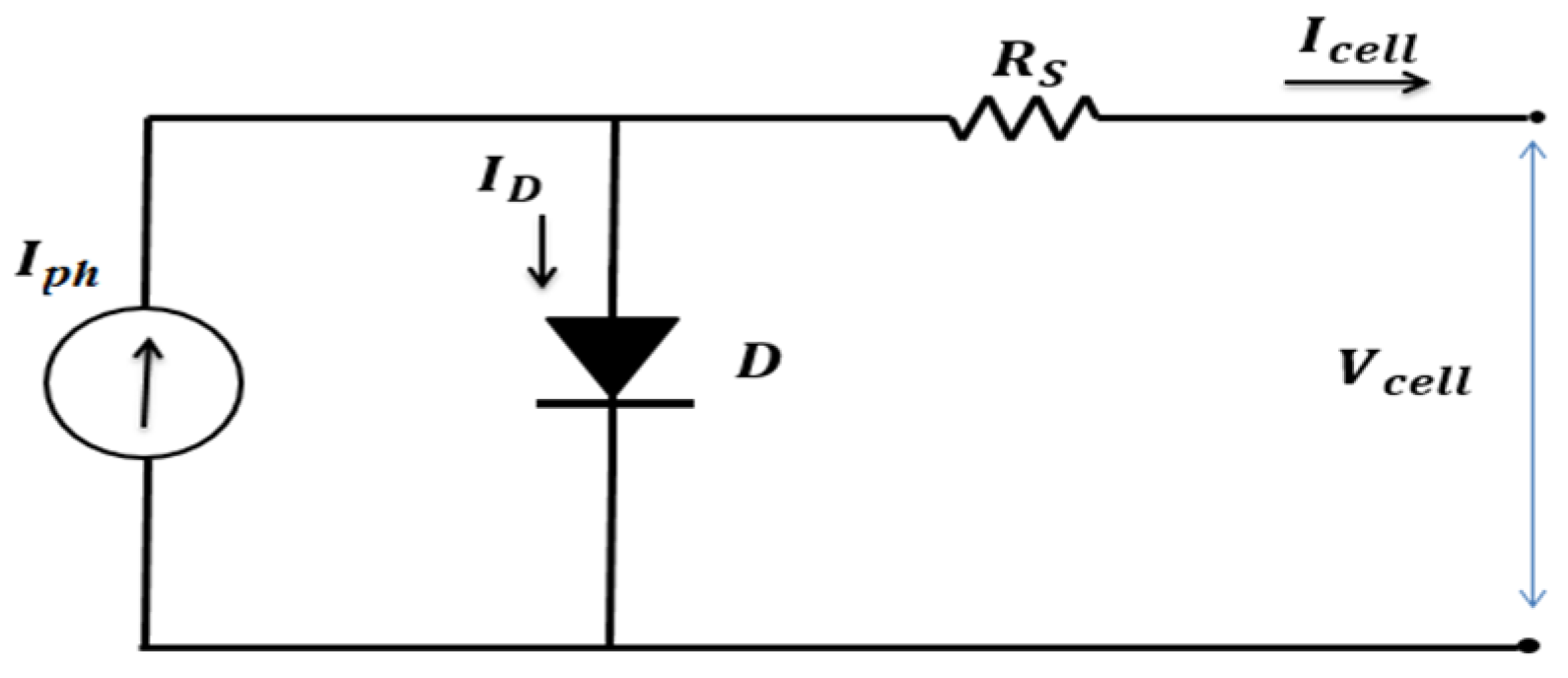
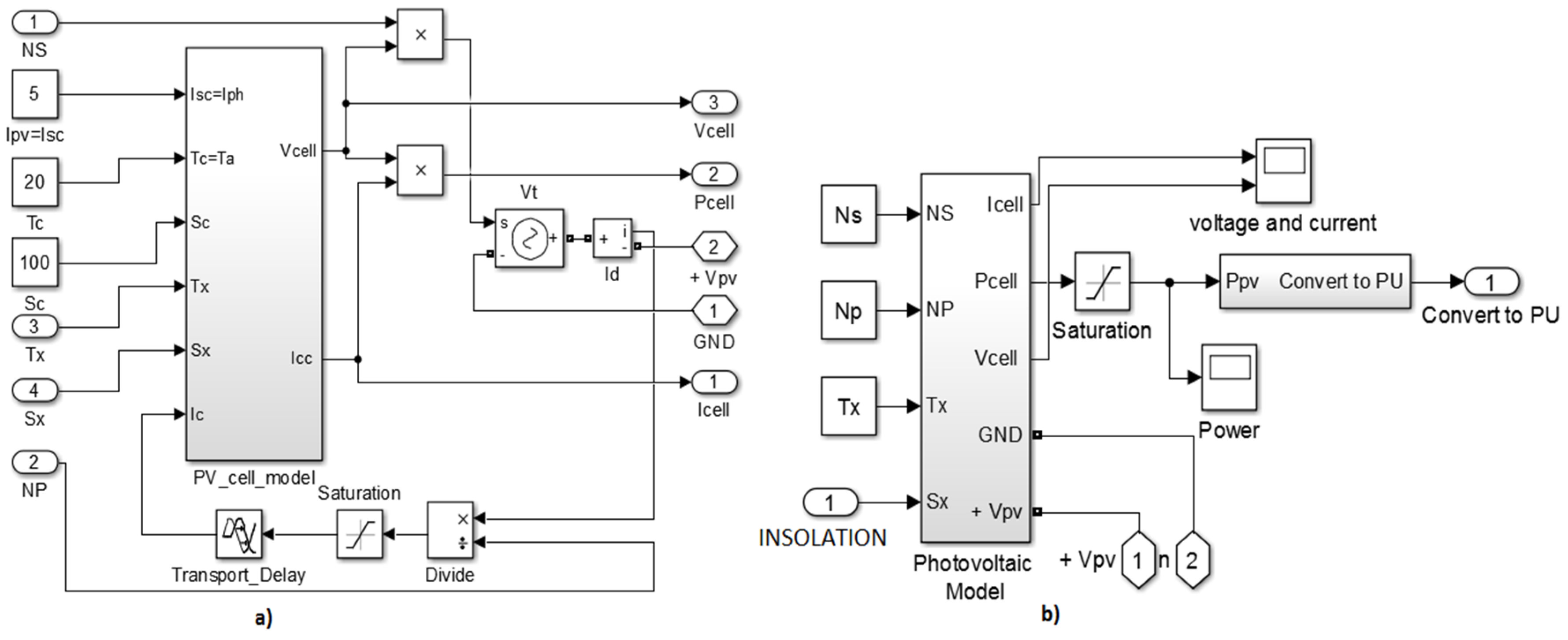
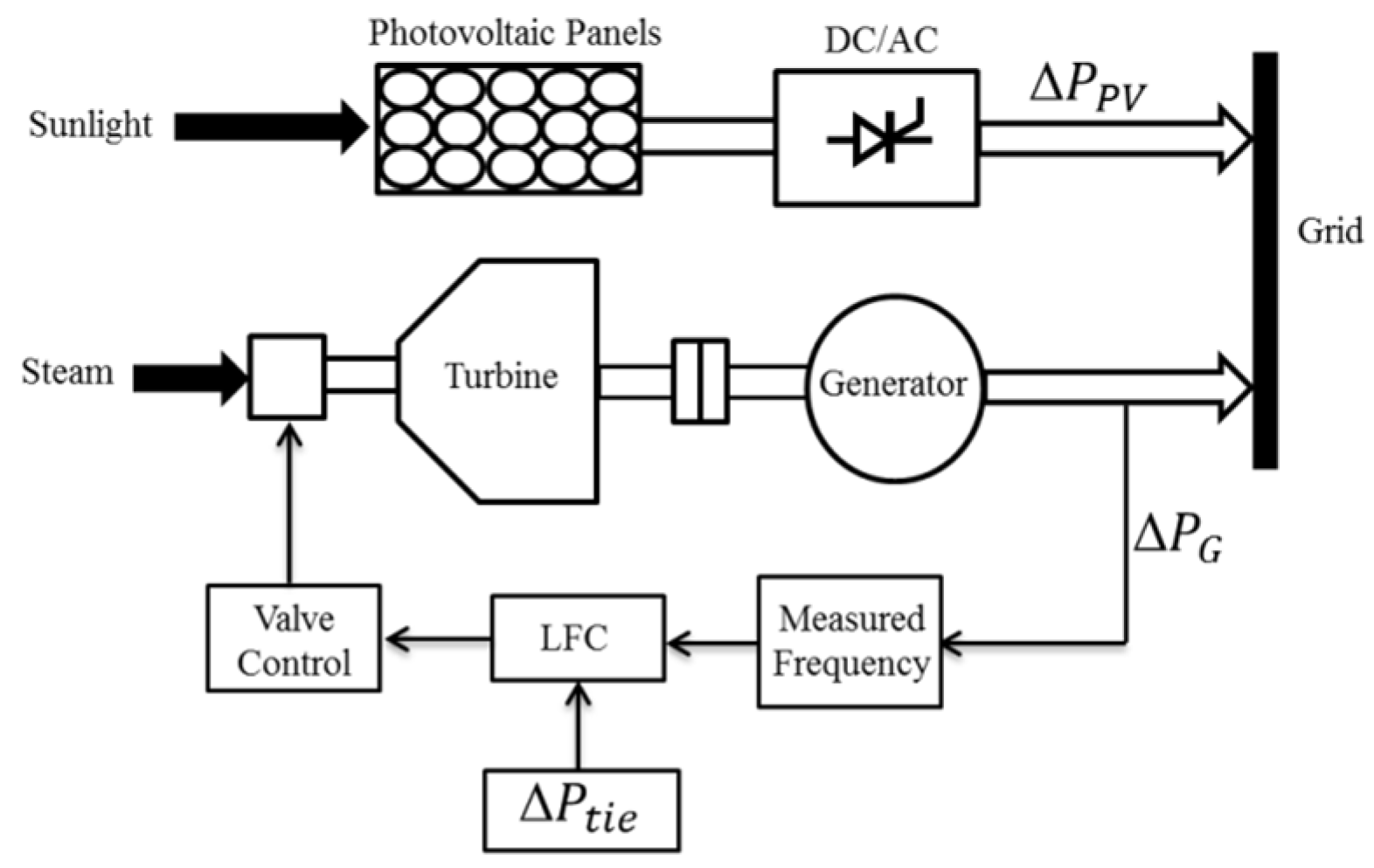
2.1.1. PV Power System

In order to determine the electrical properties of the PV-SPP, that provides the power to the interconnected system, it is necessary to observe how the current and voltage of the PV cell are affected by a variable load. When a PV cell is modelled, a sufficient number of PV cell groups ($N_S$) are connected in series, in order to generate the required output voltage. Also, a sufficient number of PV cell groups ($N_P$) are connected in parallel for generating the required output current. The PV cell variables of the equivalent circuit depend on the light intensity and temperature. Thus, the light and temperature values should be known, in order to calculate the output power [25]. The PV cell is examined, by means of Figure 2. The voltage of the PV cell can be obtained, depending on its current of it by using Equation (1). “I₀” is defined as the reverse saturation current of the diode. Definitions of the other symbols are shown in Abbreviations and Nomenclatures.

$$V_{cell}=\frac{A\times k\times T_{cell}}{e}\times \ln \left(\frac{I_{ph}+I_0+I_{cell}}{I_0}\right)$$

(1)

The operating temperature of the PV panel cells, T_cell, changes when the climate temperature and the level of solar radiation vary. Therefore, a new photocurrent and a new output voltage are generated. The operating temperature of the PV cells varies, depending on the solar radiation level and the temperature of the environment. The variable ambient temperature, T_x, affects the output voltage and the photo current of the cell. The voltage and current coefficients of these effects in the cell model are shown by C_TV and C_TI in Equations (2) and (3), respectively.

$$C_{TV}=1+{\beta }_T\times \left(T_a-T_x\right)$$

(2)

$$C_{TI}=1+\frac{{\gamma }_T}{S_{cell}}\times \left(T_x-T_a\right)$$

(3)

where T_a and T_x represent the known reference ambient temperature and the different ambient temperature at different points during the tests, respectively. For the PV-SPP model in this study, the T_x value is taken as 28 °C. The β_T and γ_T coefficients represent the slopes of changes in the cell voltage and current due to temperature, respectively. The β_T and γ_T coefficients vary, depending on the PV cell type, and are determined experimentally. β_T is calculated between 0.004 and 0.006, and γ_T is calculated between 0.02 and 0.1 [25].

Although the ambient temperature does not significantly change throughout the day, the solar radiation effectively changes because of the amount of sunlight and the cloudiness of the sky. As a result of this, the photo current, operating temperature, and output voltage of the PV cell are affected. These effects are given for the output voltage by C_SV and for the photo-current by C_SI, and are defined by Equations (4) and (5), respectively.

$$C_{SV}=1+{\beta }_T\times {\alpha }_s\left(S_x-S_{cell}\right)$$

(4)

$$C_{SI}=1+\frac{{\gamma }_T}{S_{cell}}\times \left(S_x-S_{cell}\right)$$

(5)

where S_cell is the daylight intensity used as the reference solar radiation level. S_x represents different solar radiation levels at different times, depending on the atmospheric changes. α_s is the coefficient of variation in the solar radiation level, and is defined by Equation (6).

$${\alpha }_s=\frac{\Delta T_{cell}}{S_x-S_{cell}}=\frac{T_{cell}-T_a}{S_x-S_{cell}}$$

(6)

The value of α_s is different for PV cells that do not have the same properties and this value is determined experimentally. However, this value is usually between 0.3 and 0.4 °C cm²/mW. By using the correction coefficients C_TV, C_TI, C_SV, and C_SI given above, the new output voltage V_Xcell of the PV cell and the new photo current I_XPV are calculated, as shown in Equations (7) and (8), for the new working temperature T_X and the new solar radiation level S_X. In these expressions, V_cell and I_PV are the values of the cell output voltage and the photo current at the reference cell operating temperature and solar radiation levels. A MATLAB-Simulink model of PV-SPP was explained in detail in Ref. [25]. The PV cell Simulink model used in the paper is shown in Figure 3a,b.

$$V_{Xcell}=C_{TV}\times C_{SV}\times V_{cell}$$

(7)

$$I_{XPV}=C_{TI}\times C_{SI}\times I_{PV}$$

(8)

2.1.2. Single Area Interconnected Power System

The blocks used in a single area interconnected power system are generally nonlinear systems. The loads at the operating point and the PV-SPP affect the frequency of the system. A LFC applied to a single area interconnected power system, which is shown in Figure 4, has a turbine, a generator, and other system blocks. Additionally, a PV plant generated through sunlight is demonstrated. For the system, a control responds as quickly as possible. The control process has been realized in two phases, as a primer and a seconder frequency control. The primer frequency control is achieved by adjusting the power balance with the turbine speed regulator, when there is a decrease or increase in electrical power between two different areas. The seconder frequency control is achieved by controlling the power flow between the areas, which reduces the permanent frequency error in the interconnected power system to zero.

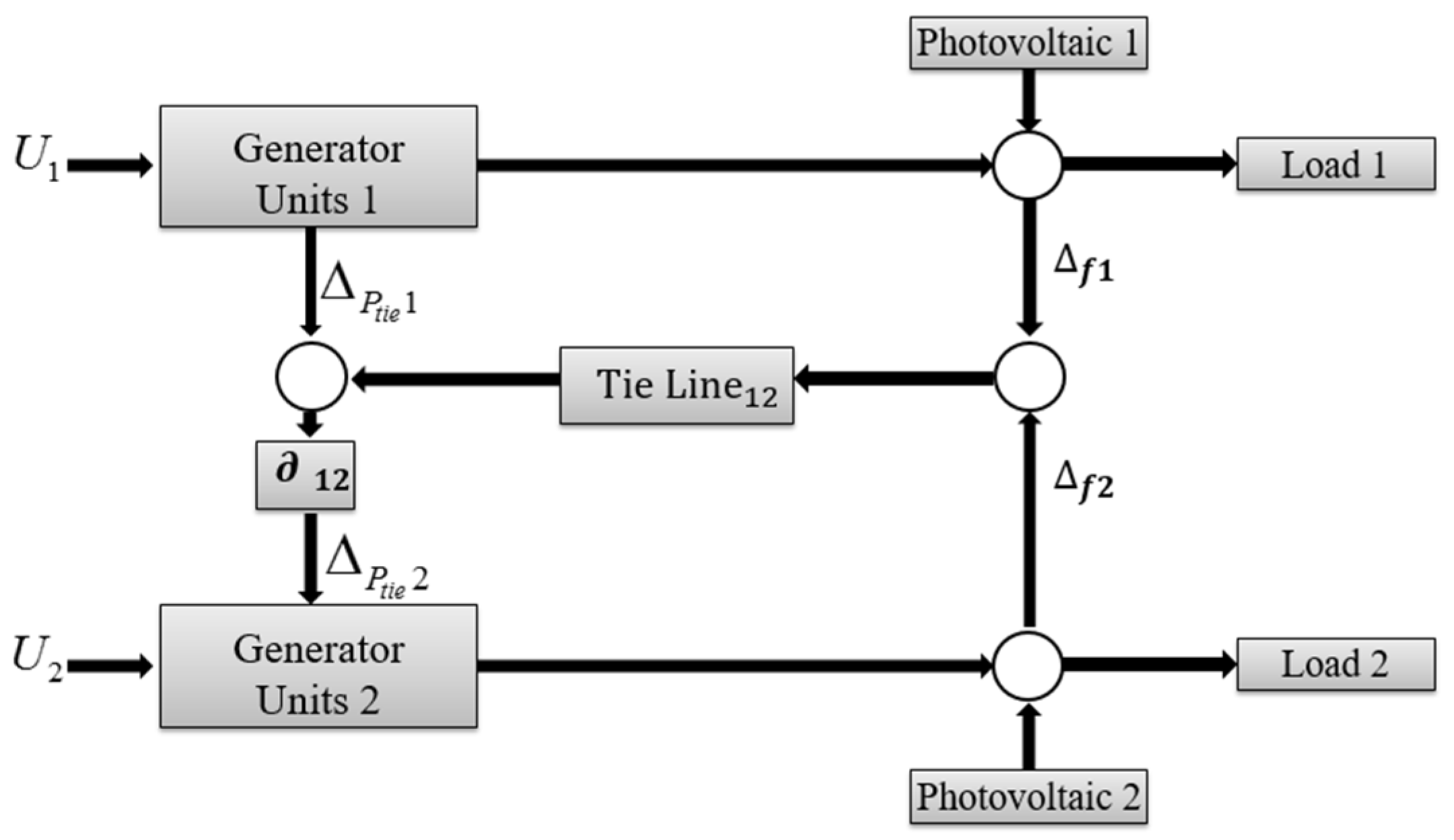
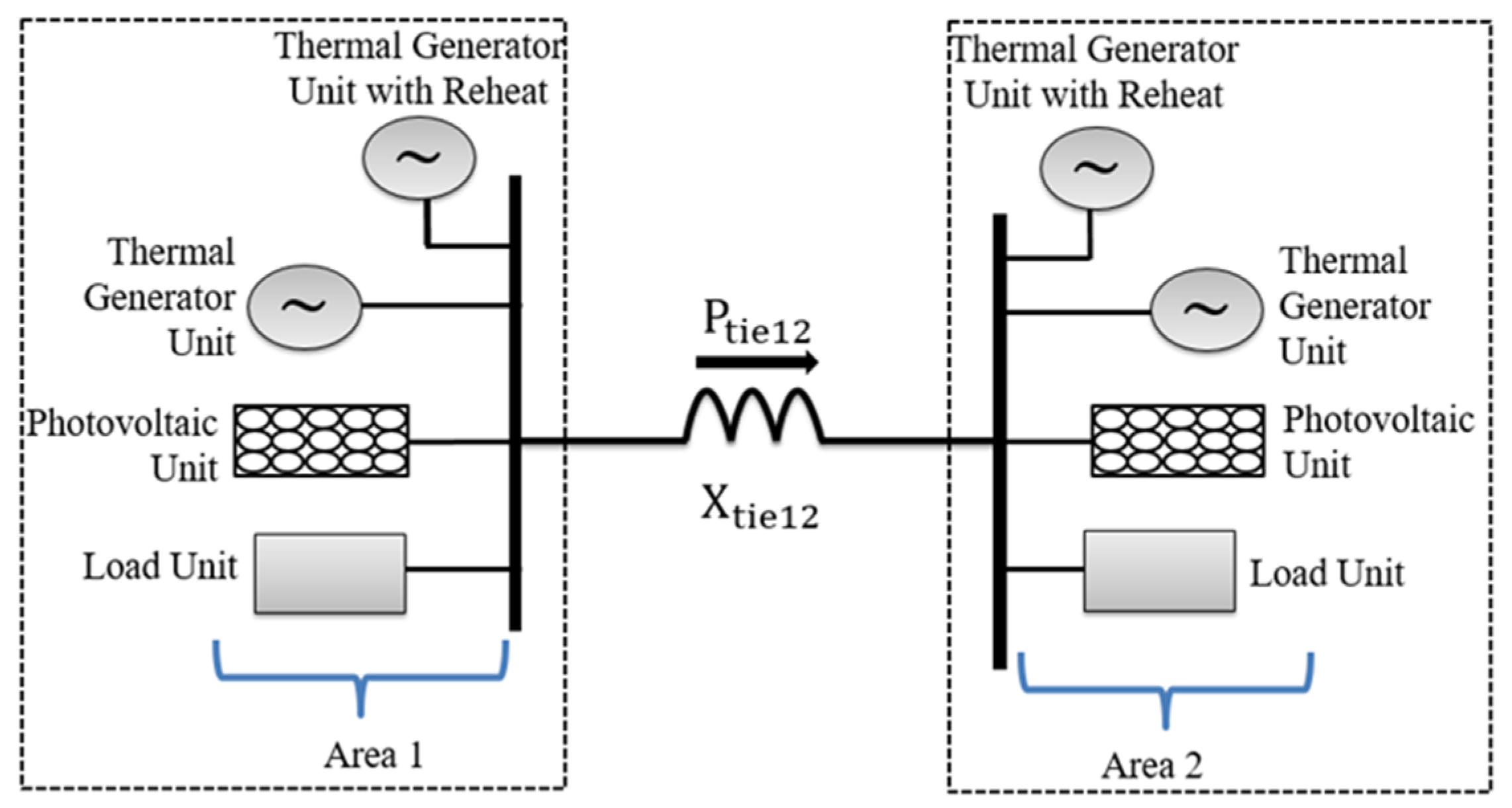
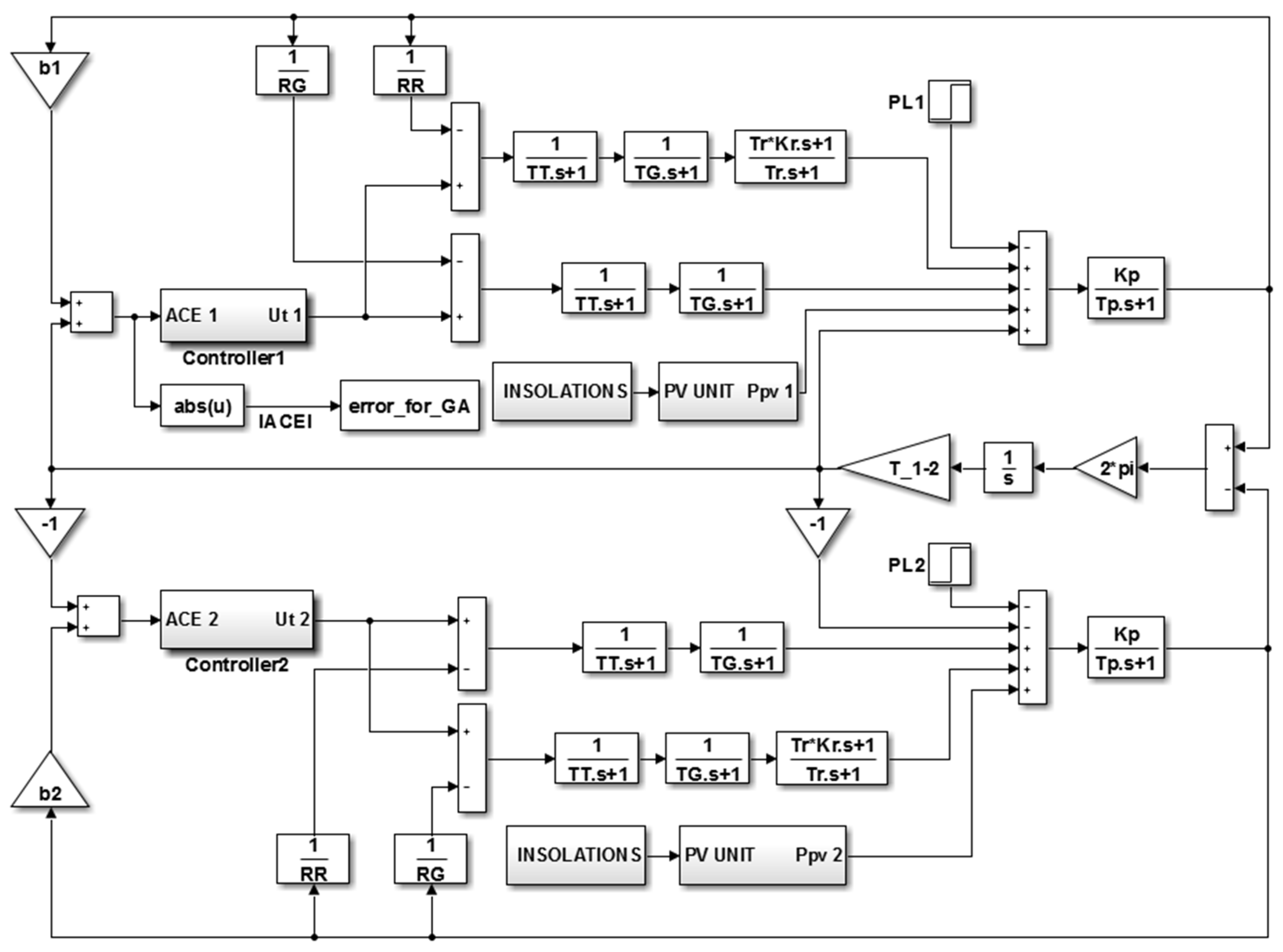
2.1.3. Two Area Interconnected Power System

A two area interconnected power system was combined with a connection link. Its block diagram, to be modelled by MATLAB-Simulink, is given in Figure 5, without a controller. In the figure, U₁ and U₂ are the control signals, $\Delta P_{tie1}$ and $\Delta P_{tie2}$ are the line power changes, and $\Delta f_1$ and $\Delta f_2$ are the input frequency deviations.

A MATLAB-Simulink model of the two area interconnected renewable energy power system is shown in Figure 6, where, $\Delta f_i$ is the frequency of the system, $R_i$ is the regulation constant, $\Delta P_{Li}$ is the load variations, $\Delta P_{PVi}$ is the power variation depending on the sunlight of the PV cell, and $U_i$ is the field controller output. The whole system with multi variable parameters is described in terms of Equations (9)–(12). Parameters of two-area power system with PV-SPP are shown in Appendix A.

$$\stackrel{.}{x}=Ax\left(t\right)+\mathit{Bu}\left(t\right)+\mathit{Ld}\left(t\right)$$

(9)

$$x\left(t\right)=\left[\Delta f_1\left(\Delta P_{\mathit{gt}1}+\Delta P_{\mathit{gtr}1}\right)\Delta P_{v1}\Delta P_{\mathit{tie}1-2}\Delta f_1\left(\Delta P_{\mathit{gt}2}+\Delta P_{\mathit{gtr}2}\right)\Delta P_{v1}\right]$$

(10)

$$u(\mathrm{t})=\left[u_1{u}_2\right]$$

(11)

$$d(\mathrm{t})=\left[\left(P_{L1}+P_{PV1}\right)\left(P_{L2}+P_{PV2}\right)\right]$$

(12)

where A is the system matrix; B and L are the input and disturbance matrices; and x(t), u(t), and d(t) are the state, control, and load change disturbance vectors, respectively.

The system output depends on the area control error (ACE), shown in Figure 6. The ACE is symbolized by Equation (14).

$$y(t)=\left[\begin{array}{c}{y}_1\left(t\right)\\ y_1\left(t\right)\end{array}\right]=\left[\begin{array}{c}\mathit{AC}{E}_1\\ \mathit{AC}{E}_1\end{array}\right]=\mathit{Cx}(t)$$

(13)

$$\mathit{AC}{E}_i=\Delta P_{\mathit{ti}{e}_j}+b_i\Delta f_i$$

(14)

where $b_i$ is the frequency bias constant, $\Delta f_i$ is the frequency deviation, $\Delta P_{tie1-2}$ is the change in the tie-line power, and C is the output matrix. $b_i$ is the expression of the frequency change in the power unit. The transfer functions used for the modelling of a turbine and a generator are given as follows [10].

$$G_{G\left(s\right)}=\frac{1}{T_{G\left(s\right)}+1}$$

(15)

$$G_{T\left(s\right)}=\frac{1}{T_{T\left(s\right)}+1}$$

(16)

In the system, a RTU type turbine was employed for increasing the efficiency of these turbines. They are made up of several turbine blades, in which the steam is reenergized between the two turbines by intermediate heaters reheating the steam. They are usually operated in the large plants [24]. The RTU transfer function Equation (17) is explained as follows [8]:

$$G_{R\left(s\right)}=\frac{{(K_R\times T_R)}_{\left(S\right)}+1}{T_{R\left(s\right)}+1}$$

(17)

The frequency stability is defined as the ability to maintain a stable frequency after an imbalance between the generated and demanded power. The power balance fails when any difference occurs on the load side or on the generation side [26]. Here, $P_{L1}$ represents the load variation of the first area. When $P_{\Delta 1}$ is non-zero, the system frequency changes. The frequency change is defined by the equations given below.

$$P_1=P_{G{t}_1}+P_{V1}$$

(18)

$$P_{\Delta 1}=P_1+P_{L1}$$

(19)

$$\Delta {\omega }_1=\frac{P_{\Delta 1}}{K_{S1}}$$

(20)

where $K_s$ is defined as the characteristic constant of the system frequency in the first area. Also, the transfer function expressing the load changes affecting the system frequency is clarified as follows [8]:

$$G_{L\left(s\right)}=\frac{1}{M_{\left(s\right)}+1}$$

(21)

To identify the ACE value, Equation (22) is used. This gives the frequency changes when a load increase of $P_{L1}$ in the first area occurs for two area interconnected power systems. Equation (23) expresses the power change in the tie line [27]. The ACE used in the FLC is calculated by means of Equations (22) and (23), as follows [24]:

$$\Delta \omega =\left(\frac{-\Delta P_{L1}}{\left(\left(\frac{1}{R_1}\right)+\left(\frac{1}{R_2}\right)+D_1+D_2\right)}\right)$$

(22)

$$\Delta P_{1-2}=\left(\frac{-\Delta P_{L1}\times \left(\left(\frac{1}{R_2}\right)+D_2\right)}{\left(\left(\frac{1}{R_1}\right)+\left(\frac{1}{R_2}\right)+D_1+D_2\right)}\right)$$

(23)

$$AC{E}_1=\left(-\Delta P_{1-2}-b_1\times \Delta \omega \right)$$

(24)

2.2. Control Methods

In this study, conventional PID, Fuzzy Logic, GA-PID, and GA-FL controllers have been used to perform the simulations. The sample time was taken as 0.001 s in all simulations. All controllers will be explained below, respectively.

2.2.1. Conventional Controllers

In the literature, proportional (P), proportional-integral (PI), and proportional-integral-derivative (PID) control methods were preferred for load-frequency control in power systems. These studies experienced some difficulties because of the sudden climatic changes and the load fluctuations [28].

In this study, a PID control has been applied to the system and is simulated by MATLAB-Simulink. The output power of PV-SPP was modelled to take into account climatic conditions. The LFC was achieved when the power obtained from the PV-SPP changed. The expression of the control signal ($u_{\left(t\right)}$) required for the PID controller is given as follows [29]:

$$u(t)=K_p\left[e(t)+\frac{1}{T_i}{\displaystyle \underset{0}{\overset{t}{\int }}e(t)dt+T_d\frac{e(t)}{dt}}\right]$$

(25)

The Ziegler-Nichols (ZN) method is used for calculating the optimum values of the parameters of the PID controller [30]. “$K_u$” is defined as the constant value of oscillation of the system and “$T_u$” is the oscillation frequency. Their formulas are given in

Table 1. ZN method of detection parameters.

Controller	${\mathit{K}}_{\mathit{p}}$	${\mathit{K}}_{\mathit{i}}$	${\mathit{K}}_{\mathit{d}}$
PID	$\frac{3\times K_u}{5}$	$\frac{6\times K_u}{5\times T_u}$	$\frac{3\times K_u\times T_u}{40}$

.

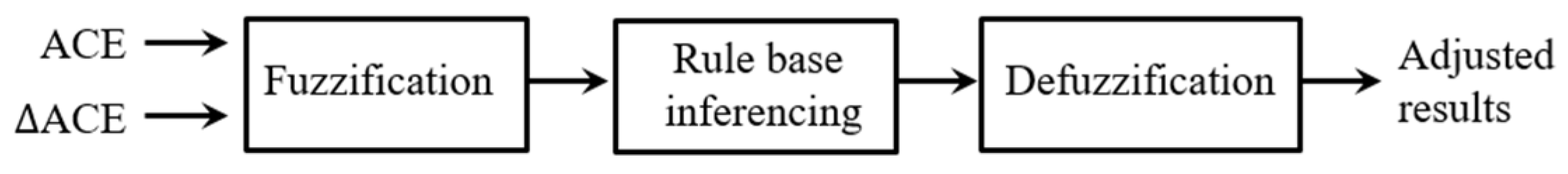
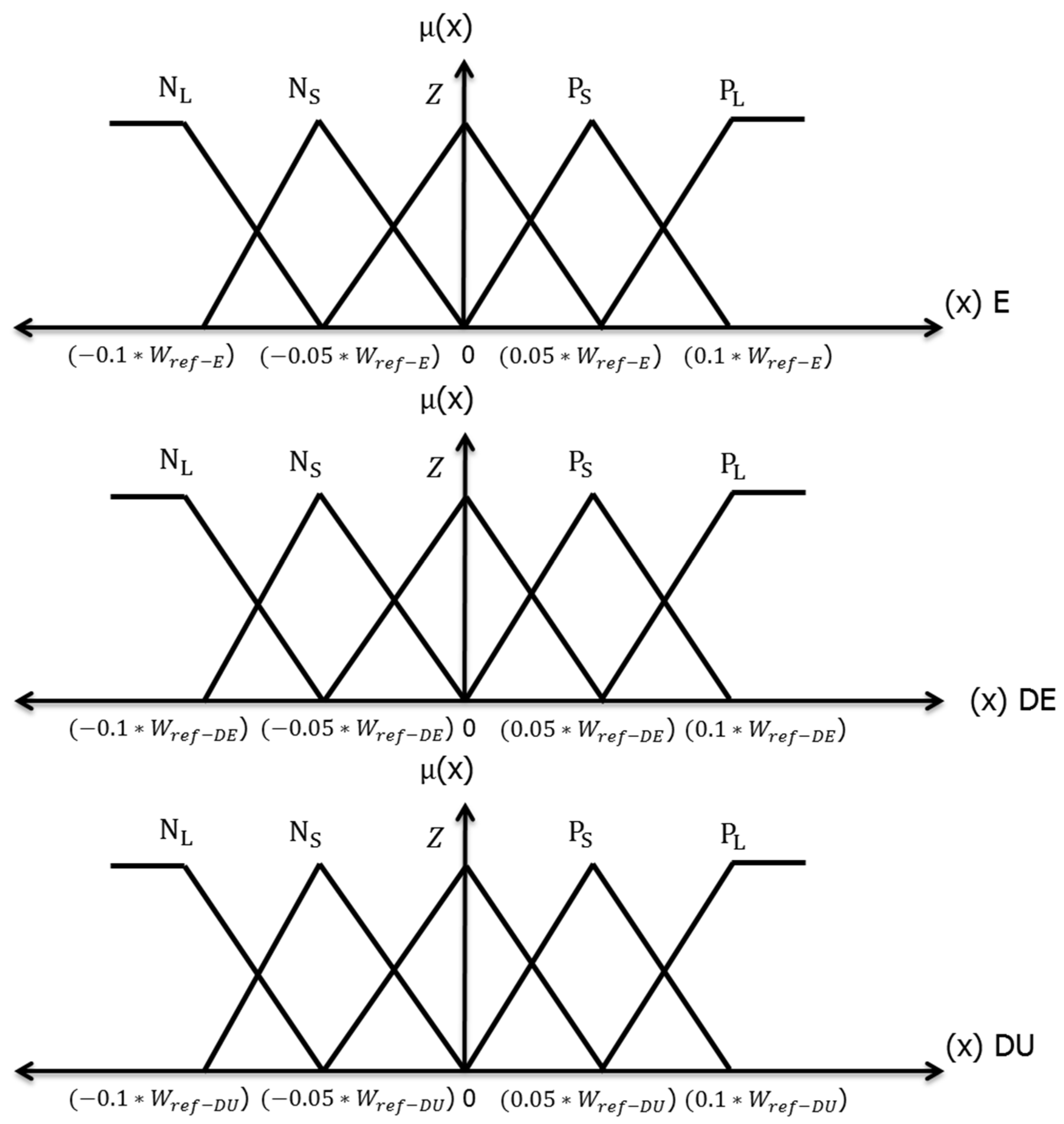
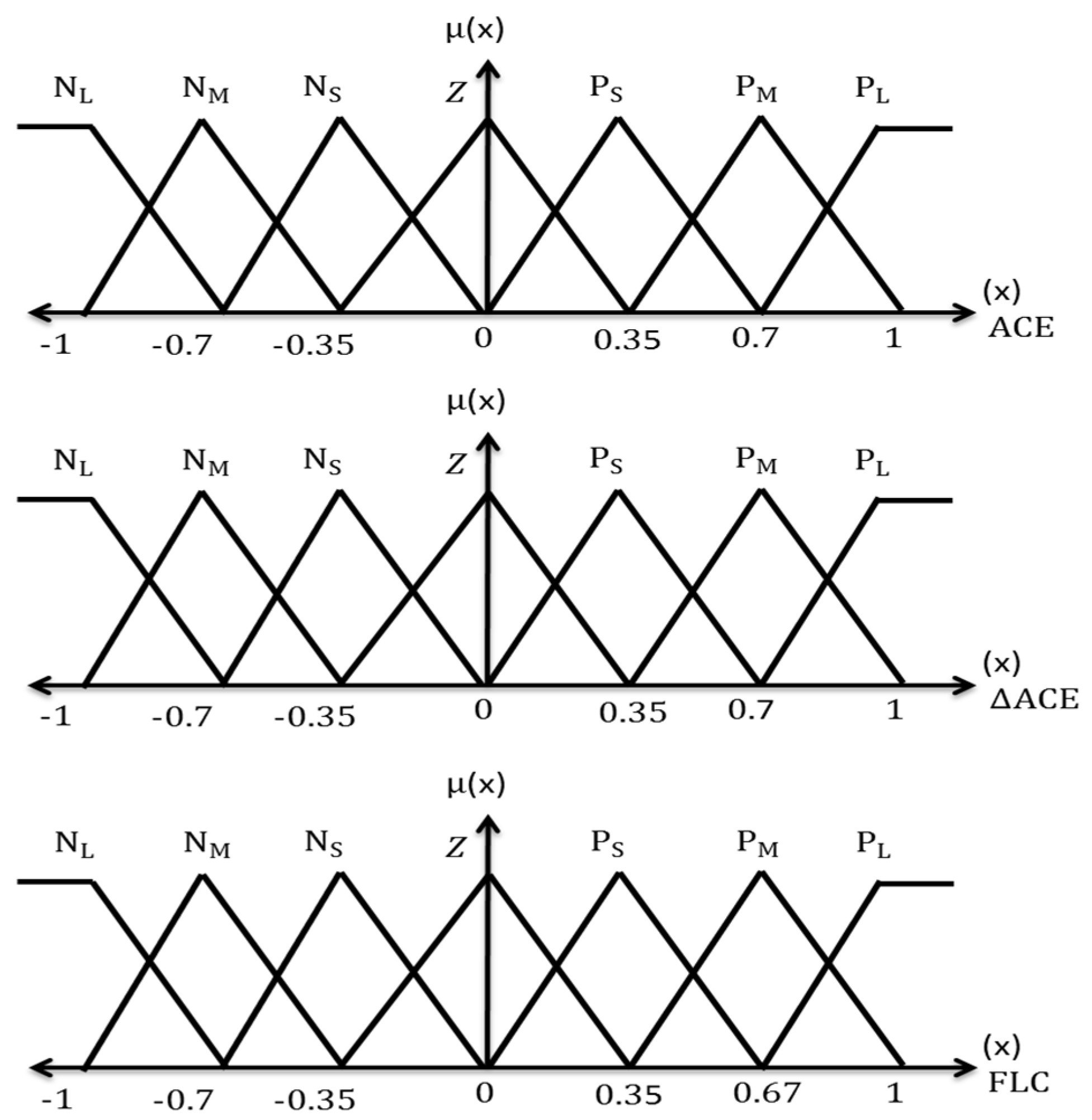
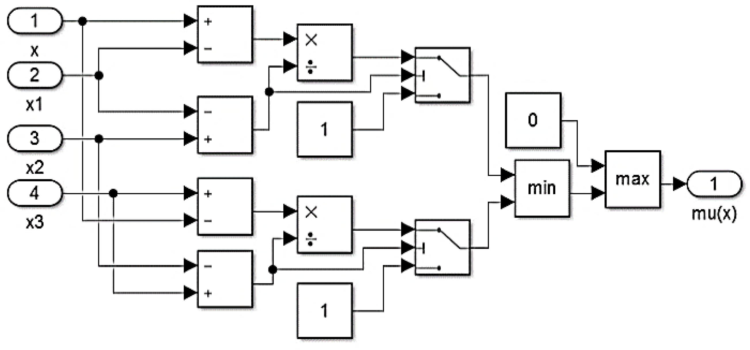
2.2.2. Fuzzy Logic Controller

Many terms used randomly in daily life have a fuzzy structure. The verbal or numerical expressions used when we are describing a thing or an event, commanding, and in many other cases, are also fuzzy. Some of these terms can be said to be young, long, short, hot, cold, hot, cloudy, partly cloudy, sunny, fast, slow, very, small, little, little, too much, etc. When an event is explained and a decision is reached in a situation, terms that do not express such certainty are used. Thanks to the fuzzy logic controller, the examination of systems gained a new perspective.

A FLC fundamentally consists of three parts. These are fuzzification, rule base inferencing, and defuzzification blocks. When modelling the FLC, error and error change signals are employed. A FLC block diagram is illustrated in Figure 7.

In this study, in order not to exceed the frequency limits, a designed fuzzy rule table is given in

Table 2. Fuzzy logic rules for FLC.

Fuzzy Logic Rules for FLC
ACE	${\mathbf{\Delta }}_{\mathit{A}\mathit{C}\mathit{E}\left(\mathit{k}\right)}$
	NL	NM	NS	Z	PS	PM	PL
NL	PL	PL	PL	PL	PM	PM	PS
NM	PL	PM	PM	PM	PS	PS	PS
NS	PM	PM	PS	PS	PS	PS	Z
Z	NS	NS	NS	Z	PS	PS	PS
PS	Z	NS	NS	NS	NS	NM	NM
PM	NS	NS	NM	NM	NM	NL	NL
PL	NS	NM	NL	NL	NL	NL	NL

N_L: large negative, N_M: medium negative, N_S: small negative, Z: zero, P_S: small positive, P_M: medium positive, P_L: large positive.

. Here, a seven stage fuzzy rule table which belongs to triangular membership functions, was formed. The regions in Table 2 were formed as three main regions: positive, zero, and negative. They were placed as two axes adjacent to each other, and their names have been given as ACE and ΔACE. Moreover, they were divided into three parts: large, medium, and small. The fuzzy logic controller has the ability to make decisions with reference to the rules in Table 2. For instance, if ACE is larger than the set value and ΔACE is rapidly increased, the output of the FLC is expected to be large.

A Mamdani fuzzy interface was used when arranging the fuzzy logic blocks. Ultimately, the output of the system approached the desired value. All other rules were obtained in a similar way. The weights of the employed triangular membership functions are demonstrated in Figure 8. These weights were found by the trial and error method, to minimize the system error.

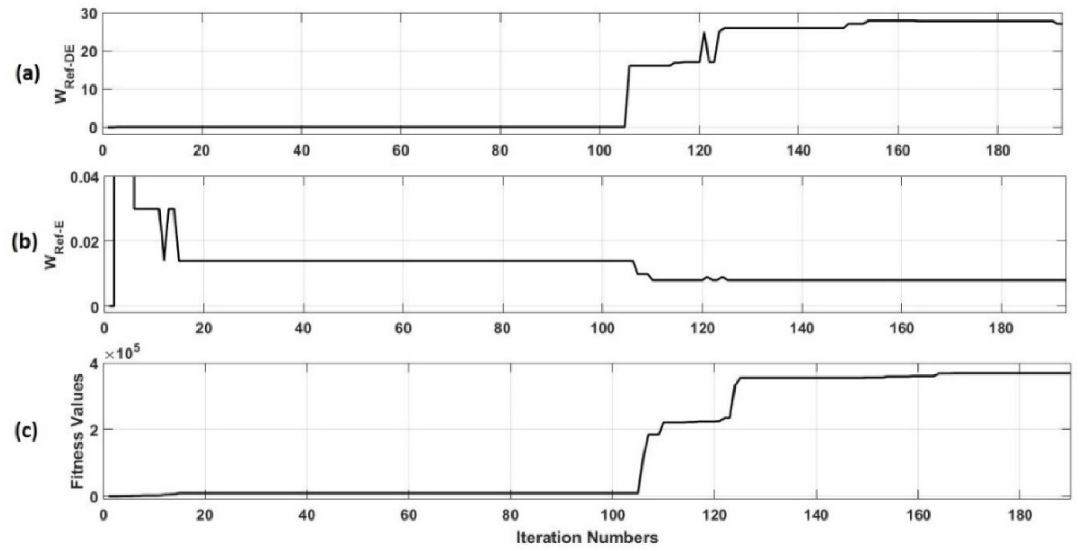
2.2.3. Genetic Optimization

GAs, being part of Evolutionary Algorithms (EA), are based on the creation of new and better solutions as a result of processes such as multiplication, mating, and mutation. They help obtain solutions in a much shorter time than conventional methods. In the same way, with GA, the best parameters of FLC and PID controllers in a sampling space are determined, and the system frequency is more rapidly set to nominal value [18].

Genetic optimization is based on a natural selection process. The algorithm repeatedly develops a population of individual solutions. This method randomly selects individuals from the current population and produces the children for the next generation. The population moves to an optimal solution over successive generations. A genetic algorithm uses three operators to generate the next generation from the current population. These operators are selection, crossover, and mutation. The individuals named as parents are selected. Crossover combines two parents to form children for the next generation. Random changes are applied to individual parents to form children by mutation. Genetic optimization processes are continued via a fitness function, defined and formulated by a GA. The correct determination of this fitness function is the most important step in solving the problem, since the frequency is unbalanced due to the insolation. It emphasizes that the determination stage of each problem has its own solution focus [31,32].

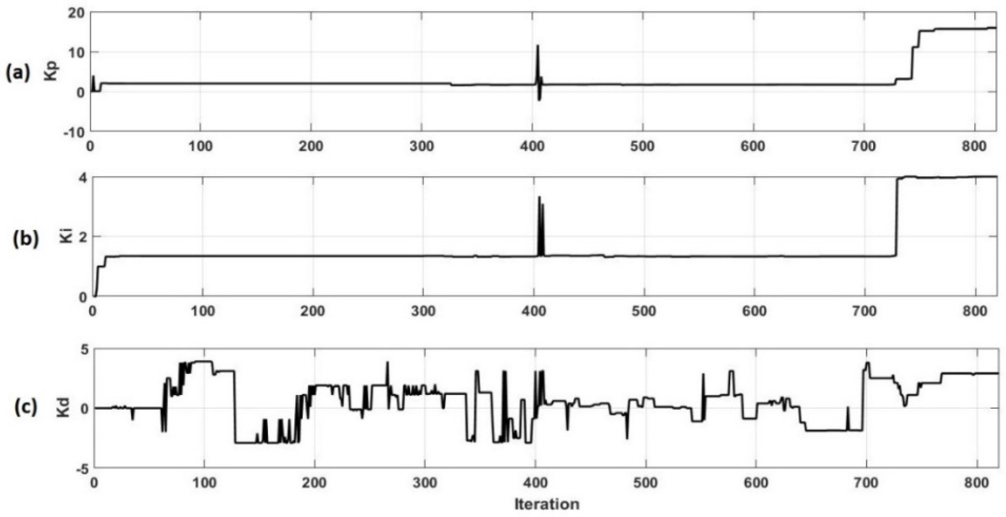
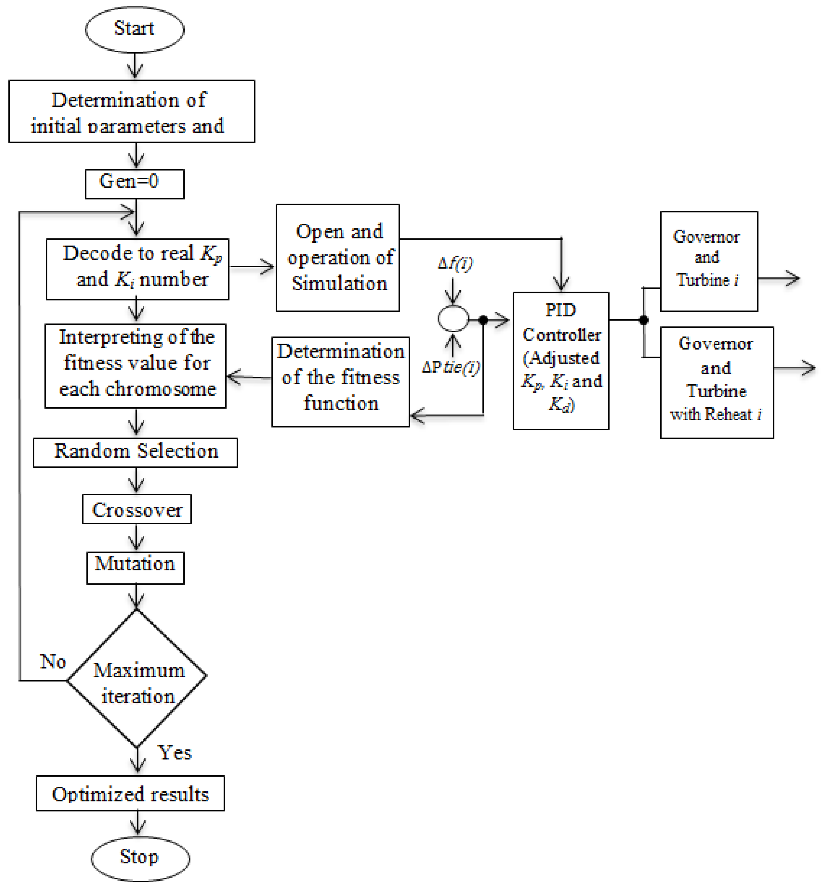
2.2.4. GA-PID Controller

Setting the parameters of a PID controller is the most important part of a control system. In this study, a GA was used to determine the parameters K_p, K_i, and K_d of the PID controller. Then, the GA-PID controller, whose parameters were defined by the GA, was modelled by MATLAB-Simulink. The modelled GA-PID controller flow diagram is shown in Figure 9.

The first step includes the forming of the initial population when the PID parameters are adjusted for the LFC. The K_p, K_i, and K_d gain parameters were calculated as applicable to the control system and as individual characteristic forms. The initial operating values were chosen to be zero, before starting the iteration. Since the LFC expresses a balance between the power in the production lines and the demanded power in the load side, the ACE value must be zero [33]. For this, the fitness function was defined as in Equation (26). The ACE value obtained at the end of each iteration was measured and sent to the GA. The GA is operated with reference to this value and new K_p, K_i, and K_d parameters were obtained to reduce the error value. At the end of each iteration, the model operated with new K_p, K_i, and K_d parameters attempts to reach a better ACE value than before. This loop was operated for more than 800 iterations. As a result of these iterations, the obtained changes in the K_p, K_i and K_d parameters are given in Figure 10. The GA parameters chosen for PID optimization are shown in

Table 3. Control Parameters of GA-PID and GA-FLC.

The GA Parameters Type	Value
Population Size	20
Initial Population	0
Crossover Rate	0.9
$K_p$ Limit	10
$K_i$ Limit	5
$K_d$ Limit	5
Mutation	8
Iteration	for PID: 800
	for FLC: 190

.

As seen in Figure 10, these parameters start to stabilize after 800 iterations. After obtaining the best K_p, K_i, and K_d parameters, the system was operated by using these values and the system results were obtained. The fitness function for the GA-PID controller is given as follows:

$$F\left(f\right)=\left[\frac{0.5}{average\left[absolute\left(GA-PID(AC{E}_1\right)\right)]}\right]$$

(26)

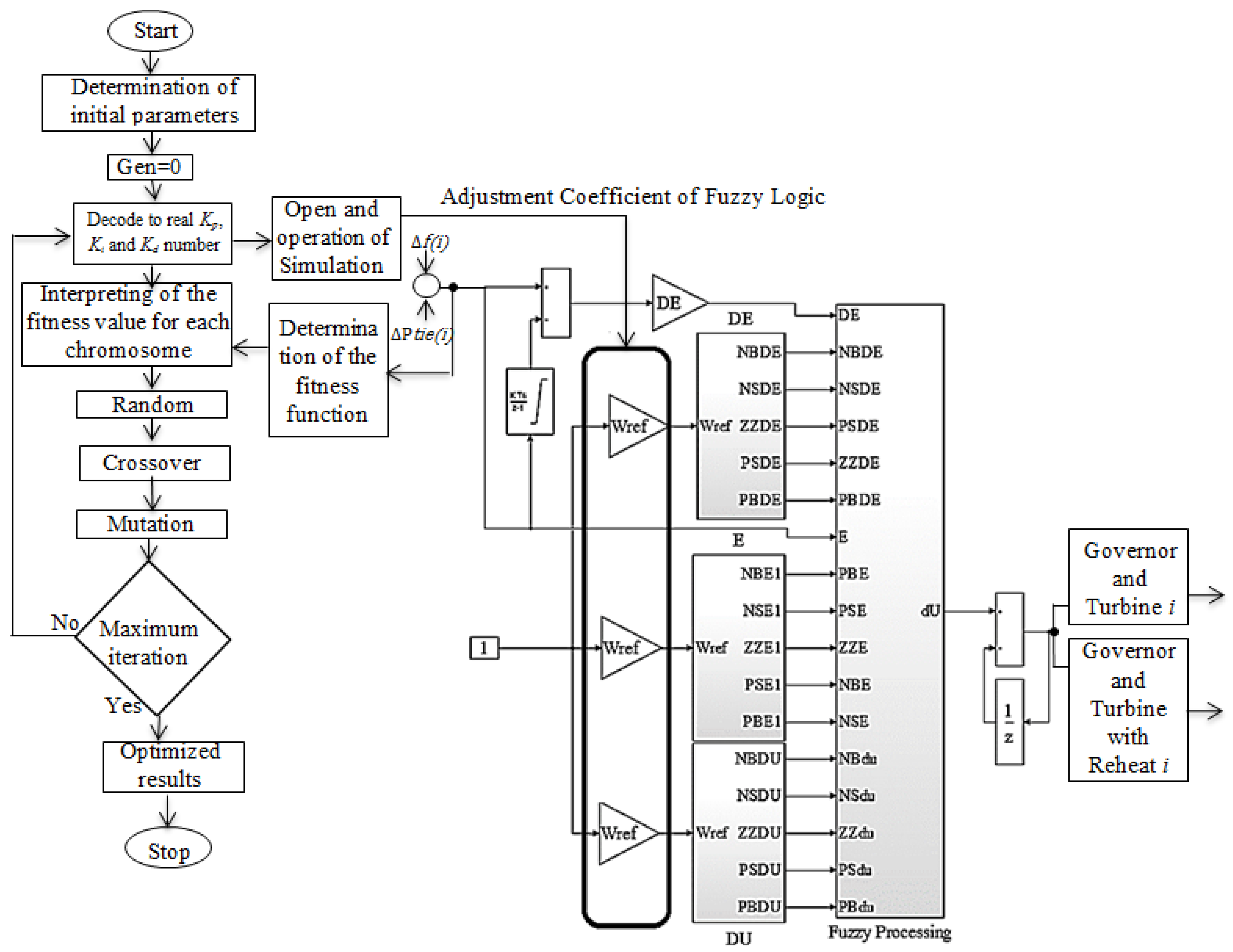
2.2.5. GA-FLC Controller

In this study, a new FLC approach (GA-FLC) which has GA optimized weights, has been proposed for the LFC in two area multi source interconnected renewable energy power resources. A block model of the developed GA-FLC could be easily adapted to different systems and could save time when designing these systems. Moreover, for users, the developed GA-FLC could provide the possibility to make changes, through entering the model content into the controller. The control error E is the fundamental element of the two dimensional space DE, which is the variation of this error in a sampling process. The GA parameters chosen for the FLC optimization are shown in Table 3.

The input and output blocks of the GA flow diagram and the FLC model of the new proposed GA-FLC are presented in Figure 11. Here, the first and most important step is to compose these fuzzy membership functions for the input and output sections of the fuzzy space. To carry this out, the equation of the triangular membership function is described, as in Equation (27).

$$\mu \left(x\right)=max\left[min\left(\frac{x-x_1}{x_2-x_1},\frac{x_3-x}{x_3-x_2}\right),0\right]$$

(27)

In addition, a MATLAB-Simulink model of the triangular membership function is illustrated in Figure 12.

Here, $X_1$, $X_2$, and $X_3$ are the precise parameters used to determine the location and region of the triangle [34]. This triangle membership function has been operated in both the fuzzification and defuzzification processes. Altas and Sharaf [34] provided detailed information for composing the FLC algorithm via MATLAB-Simulink.

In this study, for the new proposed GA-FLC, the required weights were individually determined for error E, error change DE, and the defuzzification membership functions. For this purpose, the GA was used and the process was repeated in every simulation. The triangular membership functions used these weights and are depicted in Figure 13. Moreover, these changes in the triangular membership function weights and the fitness value of the new proposed GA-FLC are given in Figure 14.

The new weights $W_{ref-E},W_{ref-DE}$, and $W_{ref-DU}$ have been determined, depending on the error value derived from each iteration and the GA. For the next iteration, the system frequency changes have been observed using these values. The fitness function required for this solution has been governed in a similar manner, by Equation (26). The fuzzy logic rules, including the five rules of the new GA-FLC, are offered in

Table 4. The five fuzzy logic rules of the new GA-FLC.

Fuzzy Logic Rules for GA-FLC (5)
ACE	∆ACE(k)
	NL	NS	Z	NS	NL
$N_L$	$N_L$	$N_S$	$N_S$	$N_S$	Z
$N_S$	$N_S$	$N_S$	$N_S$	Z	$P_S$
Z	$N_S$	$N_S$	Z	$P_S$	$P_S$
$P_S$	$N_S$	Z	$P_S$	$P_S$	$P_S$
$P_L$	Z	$P_S$	$P_S$	$P_S$	$P_L$

. Here, a rule table with five rules instead of seven rules has been utilized, in order to reduce the problem of slowing down the system, which is a combination of the GA and the FLC. The system has been independently run 30 times, to ensure the validity of each result, and is shown in

Table 5. Optimization results for over 30 independent runs of GA-PID and GA-FLC.

Controller	Controller Parameters	Min.	Mean	Median	Max.	Standart Deviations
GA-PID	$K_p$	6.4295	13.6868	15.4255	15.9988	2.8714
	$K_i$	3.8590	7.5896	7.8589	7.9999	0.7833
	$K_d$	0.4094	2.8252	2.4297	6.4565	1.2078
GA-FLC	$W_{ref-DE}$	0.1369	0.4931	0.4588	0.8591	0.1391
	$W_{ref-E}$	0.0086	0.1761	0.1262	0.9371	0.1986
	$W_{ref-DU}$	0.1000	1.2374	0.7393	5.3660	1.4304

.

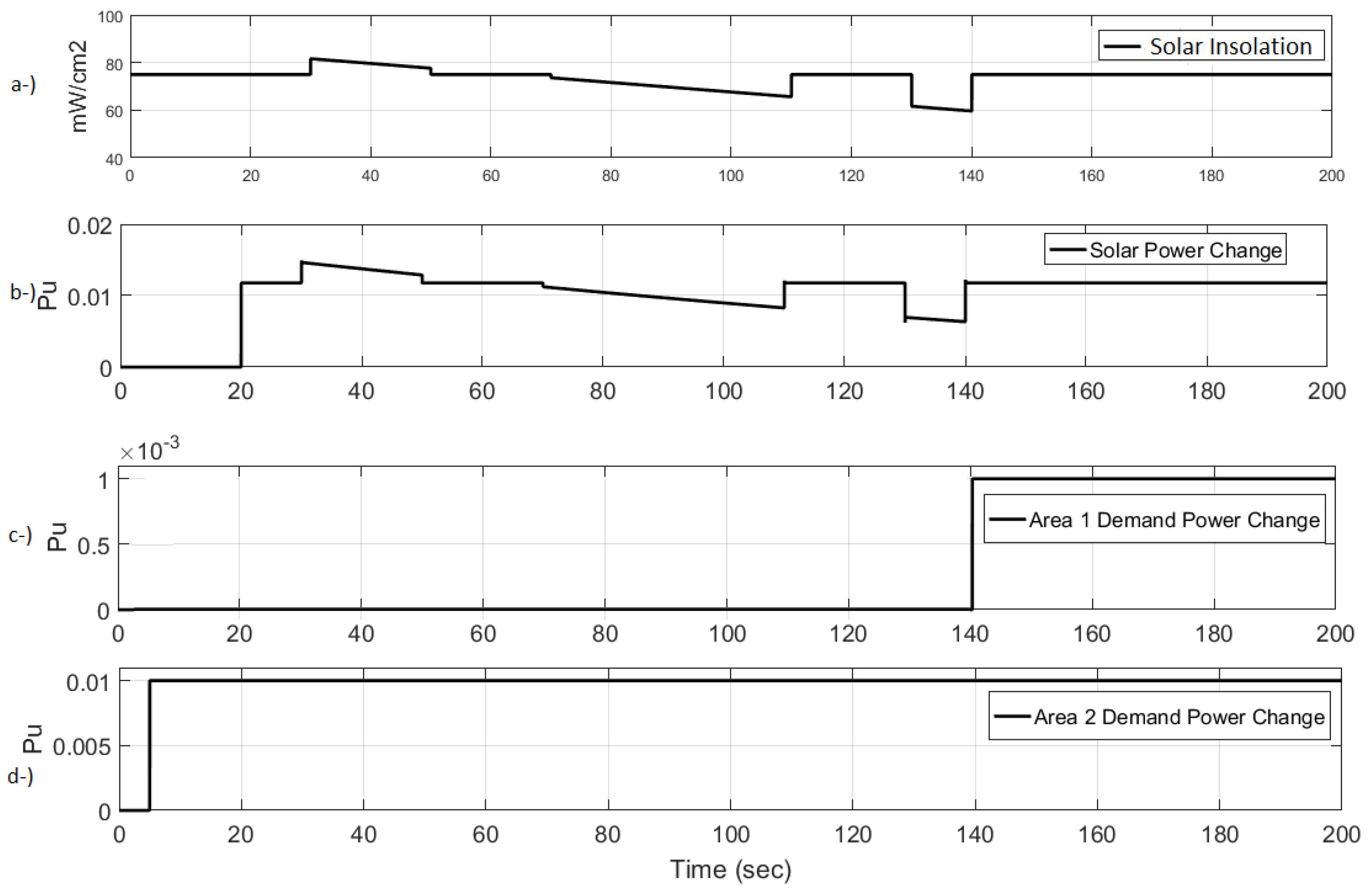
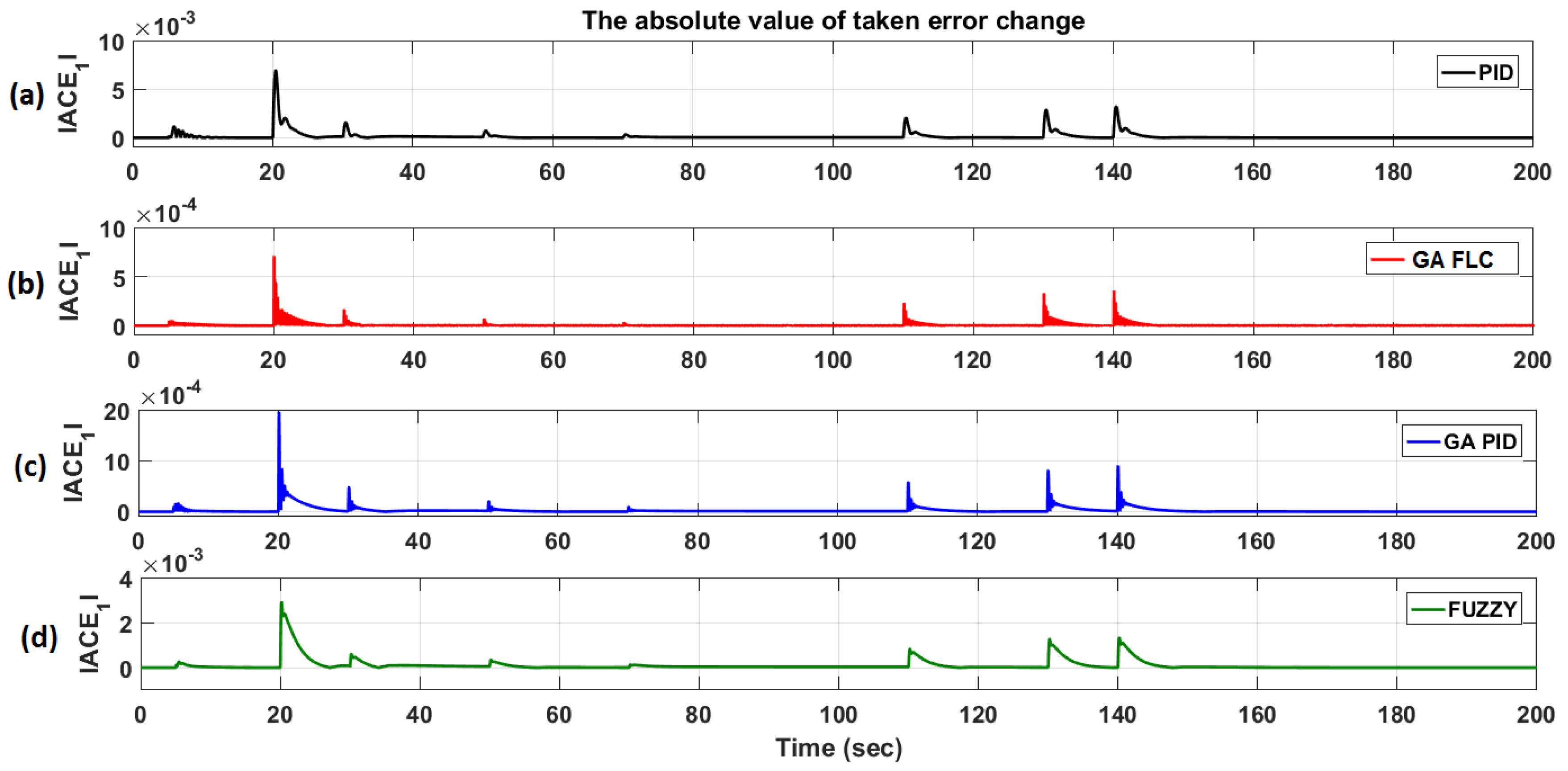
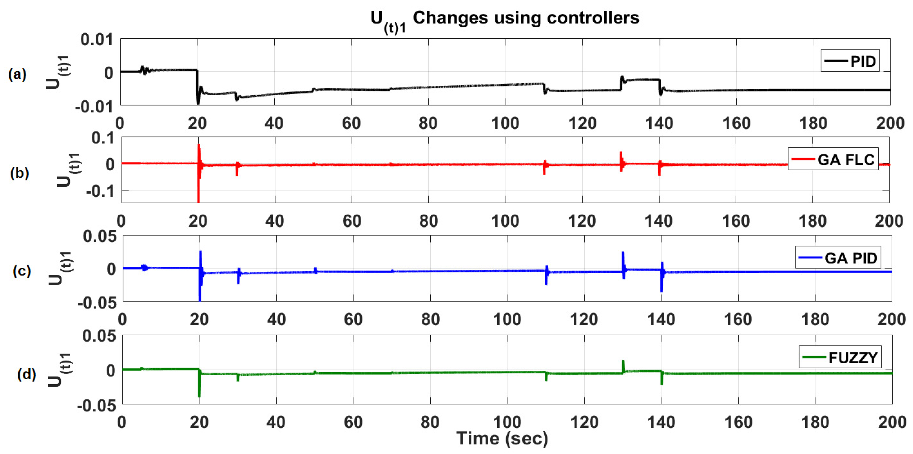
3. Results and Discussion

In this study, a PV-SPP was added to the two area multi source interconnected power system. The LFC of the system was carried out to compare a PID, a GA-PID, a FLC, and the new proposed GA-FLC results. The results obtained from these comparisons are given below. When the control process is performed, a model that gives a power increase value of 0.001 P_u in area 2 for the demanded power at the 5th s. and a power increase value of 0.01 P_u in area 1 for the demanded power at the 140th s., were formed. In addition, the fluctuations of the generated power from the solar energy plants inserted in both areas depending on the climatic conditions, starting from the 20th s., were modelled. In Figure 15, these fluctuations of solar energy plants are depicted.

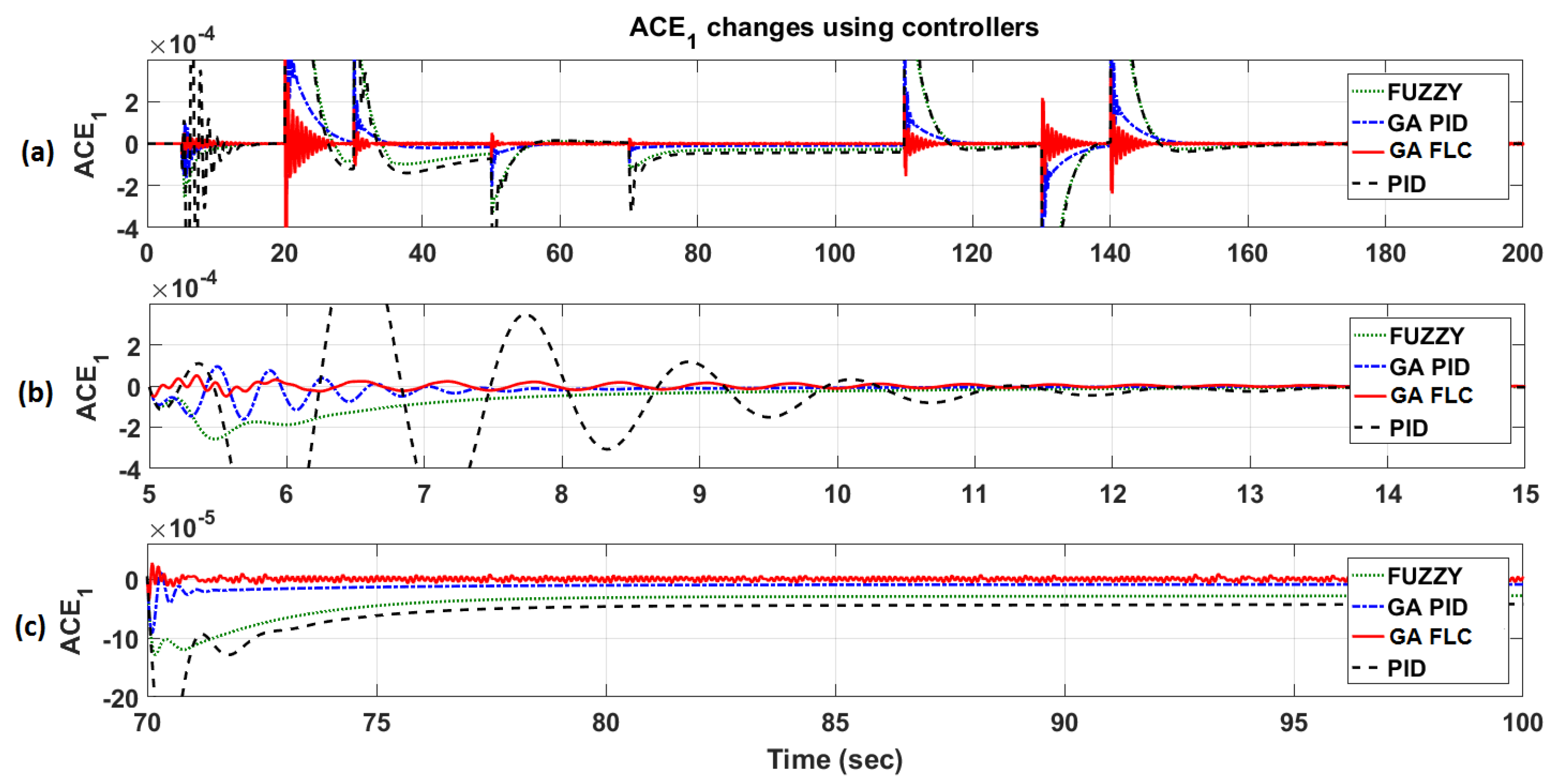
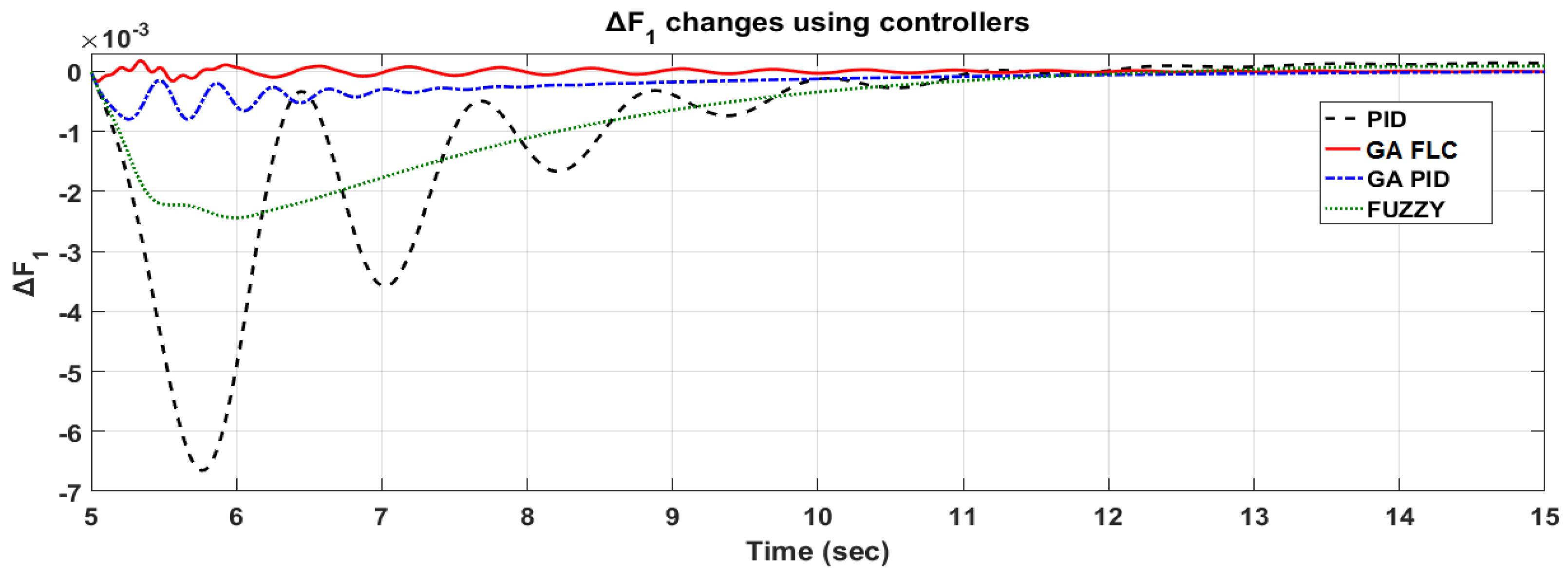
3.1. Results and Discussion for Area 1

The modeled system has been operated for 200 s. The changes of ACE₁ for area 1 are shown in Figure 16. In Figure 16b, the effect of increasing the demand power in area 2 on the frequency in area 1, is demonstrated. According to the results obtained from the four different controllers, the GA-FLC demonstrates a better performance than the others, in terms of the sudden oscillations. Additively, Figure 16c illustrates the effect of a long-term power drop of the solar power plant due to climatic conditions on the ACE₁ value. According to the results of Figure 16, the proposed GA-FLC could set the desired value within certain limits, such that there is hardly any oscillation. In

Table 6. The obtained results.

Parameters	Designs Controller	Area 1 Loads Increase (5th s)		Area 1 Solar Power Decrease (70th s)		Area 2 Loads Increase (5th s)
		Overshoots	Settling Time	Overshoots	Settling Time	Overshoots	Settling Time
ACE	PID	−0.00114	13.1	−0.00032	80.5	−0.00655	8.9
	FL	−0.00025	8.6	−0.00012	78.5	−0.00267	8.4
	GA-PID	−0.00016	6.8	−0.00009	71.5	−0.00177	5.8
	GA-FLC	−0.00005	5.5	−0.00003	70.6	−0.00069	5.1
Δf	PID	−0.00665	9.6	−0.00077	76.1	−0.00128	9.6
	FL	−0.00244	9.1	−0.00031	73.4	−0.00381	8.3
	GA-PID	−0.00078	6.7	−0.00021	70.5	−0.00556	5.9
	GA-FLC	−0.00018	5.1	−0.00008	70.1	−0.01224	5.5
Δtie1−2	PID	0.00207	-	-	-	-	-
	FL	0.00084	-	-	-	-	-
	GA-PID	0.00024	-	-	-	-	-
	GA-FLC	0.00002	-	-	-	-	-

, the obtained results are presented. The proposed GA-FLC also exhibited the best performance, with a settlement time of 5.5 s. from the 70th s, as indicated in Table 6. It is also seen that the GA-FLC has a better value as $0.06\times {10}^{3}Pu$, when compared to other controllers at the 70th s. In Figure 17, variations of the absolute value of the ACE₁ value for area 1; (a) PID; (b) GA-FLC; (c) GA-PID; and (d) FLC, are demonstrated. The reason why the absolute value of the ACE₁ is displayed is that the reference error variance of the system used in the GA processes could be seen from zero, to how much it changes in the positive direction. In addition, the ACE₁ signal, which is controlled by four different controllers, was converted to the form, $U_{\left(t\right)1},$ in Figure 18, and was then transferred to the governor and the turbines to balance the frequency value. The purpose of this is to observe which signals sent to the turbines and the generators are more effective. The $U_{\left(t\right)1}$ signals obtained from the controllers are shown in Figure 18. As shown in Figure 18b, GA-FLC produced a wider and higher frequency value. This is due to the use of more mathematical functions while modelling the GA-FLC in a Simulink environment. With frequency damping blocks, this high frequency signal can be prevented from damaging the turbine valves. Moreover, Figure 19 shows that the frequency value in the interconnected network controlled by the proposed GA-FLC is better than the other control methods. The effect of a load increase in area 2 on area 1 was shown to be minimized. Furthermore, the frequency oscillations of the proposed GA-FLC were shown in this way, which shows the frequency value in the interconnected network, to be kept at the minimum value. The best results obtained by GA-FLC have also been reached by a settling time of 5.1 s and an overshoot value of −0.00018 P_u, as indicated in Table 6.

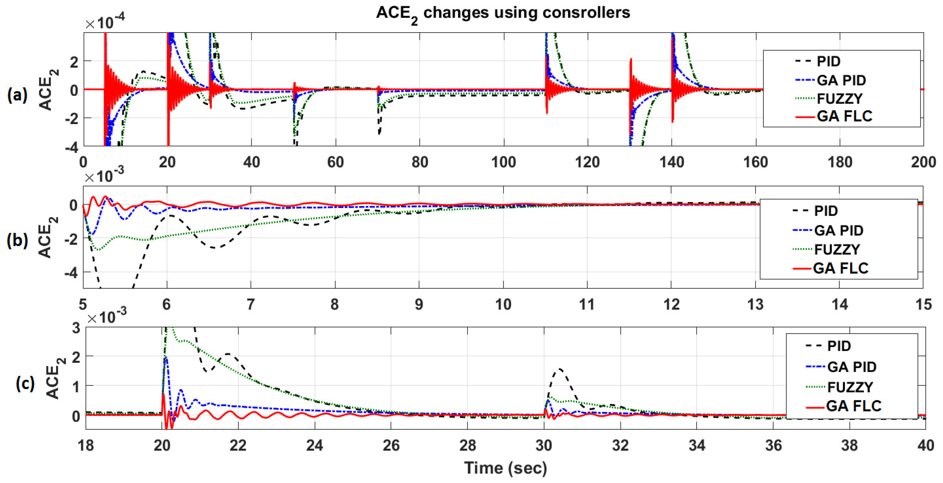
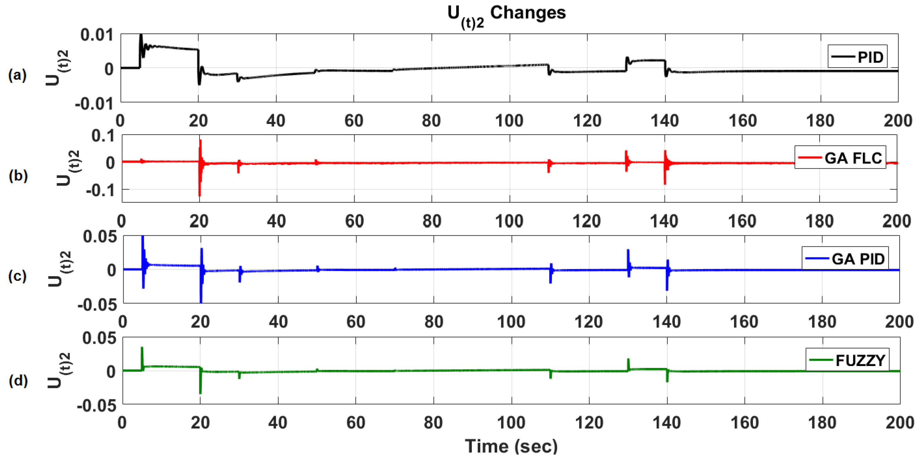
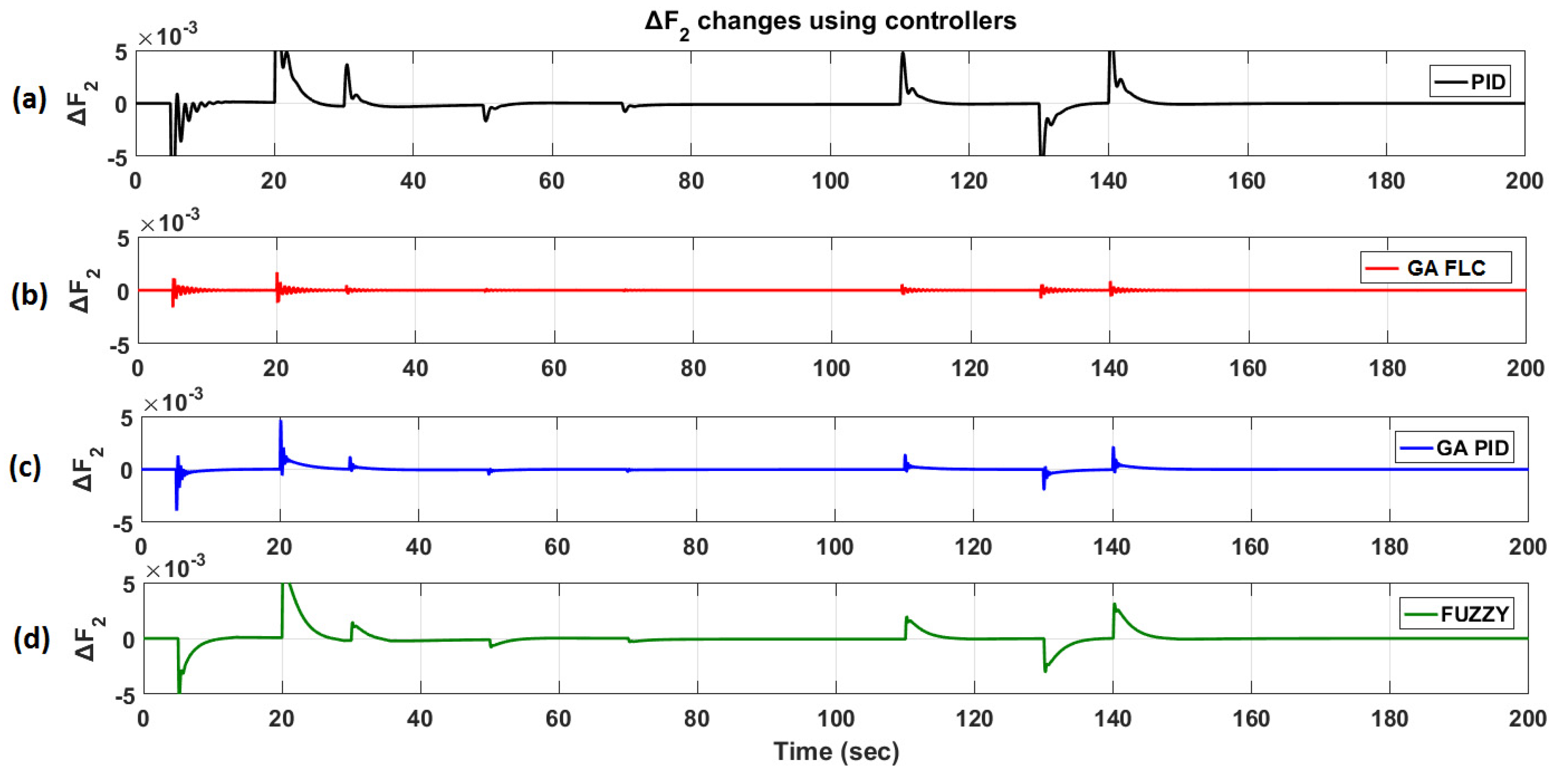
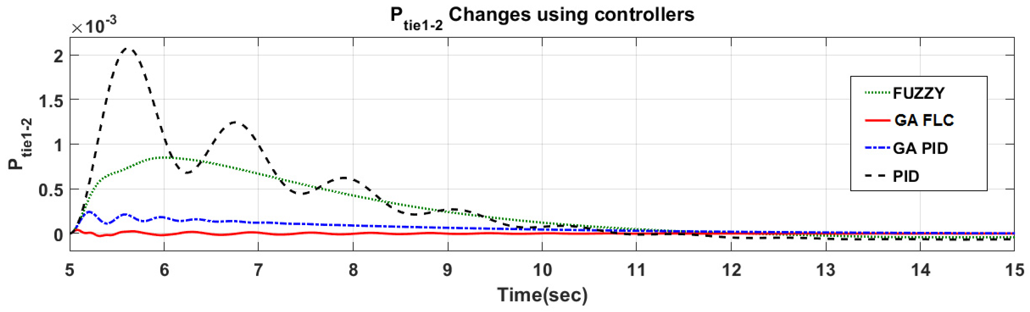
3.2. Results and Discussion for Area 2

Detailed simulation results of the interconnected network in area 2 are given in Figure 20, Figure 21 and Figure 22. The variations of ACE₂ values throughout the entire simulation are illustrated in Figure 20a and the special cases are shown in Figure 20b,c. Here, the case of both sudden load fluctuations and the responses of the system variables for long-term power reduction in solar power plants, are observed. As noted in Table 6, the proposed GA-FLC reached a settling time value of 5.1 s and then quickly minimized the error. In addition, the proposed GA-FLC provided at least three times more overshoot than the GA-PID controller, as shown in Figure 20b and Table 6. In Figure 21, $U_{\left(t\right)2}$, as the new status after controlling the ACE₂ value, is demonstrated. The results of the PID, GA-PID, FLC, and the proposed GA-FLC controllers modelled to minimize the frequency variation, ΔF₂, in area 2, are revealed in Figure 22. In Figure 22b, it is shown that the GA-FLC maintains a balanced frequency in the second region. The power change over the connection line between area 1 and area 2 is shown in Figure 23. As shown in Figure 23 and Table 6, the frequency deviation in the second area is minimized. When the situation at the 5th s is examined, the settling time value of the GA-FLC is set to 5.5 s, GA-PID is set to 5.9 s, FL is set to 8.3 s, and PID is set to 9.6 s.

When the responses given by the controllers to the situation caused by the decrease in power at the 70th s in the solar power plant are examined, it is seen that the settling time value of 70.1 s obtained by the proposed controller is the fastest and best result.

4. Conclusions

In this paper, a new GA-FLC controller was proposed for frequency stability problems in a two area multi source interconnected power system. The power system to be controlled was consisted of a thermal, a reheated thermal, and a PV unit. In addition to the proposed controller, conventional PID, FL, and GA-based PID controllers were designed. All systems and controllers were designed and simulated with the Matlab-Simulink program. In the simulations, a change in the frequencies and the tie-line power were observed by implementing each controller. Since there was a two-area power system and they were connected by a tie-line, the outputs of $\Delta F_1$, $\Delta F_2$, and $\Delta P_{tie}$ of the system were individually plotted. As can be seen from the data in Table 6, the proposed controller produces better results than the other controllers, both in terms of overshoot and settling time values. These values were taken during the load increase and the solar power decrease periods. Therefore, this demonstrates the reaction of the system at the moment of operation and a more realistic simulation was realized. The proposed GA-FLC has three membership functions with an optimized GA, and twenty-five rules. Owing to the proposed controller, the system frequency is affected at a minimum rate when the power changes on the PV-SPP because of climatic conditions. Moreover, the ability of the system to adapt to sudden power fluctuations at the operation point was also improved. In the meantime, the optimum values of the $K_p$, $K_i$, and $K_d$ parameters for the PID controller were determined by the Zigler-Nichols method.

In conclusion, the frequency stability problem caused by solar energy sources in the interconnected power systems was abolished. According to these results, for the frequency stability, the proposed GA-FLC yielded an efficiency of about 90% compared to the conventional PID controllers. Moreover, it was observed that the overshoot value of the proposed control technique was 75% better than the FLCs, and approximately 40% better than the GA-PID controllers. Ultimately, since the the overshoot values and the settling time values directly affect the operating lifetimes, operating costs, and efficiencies of the grid, the proposed GA-FLC would be beneficial and advisable for an interconnected power system with solar power sources.

References

1. Goksenli, N.; Akbaba, M. Development of a new microcontroller based mppt method for photovoltaic generators using akbaba model with implementation and simulation. Sol. Energy 2016, 136, 622–628. [Google Scholar] [CrossRef]
2. Chandra Sekhar, G.T.; Sahu, R.K.; Baliarsingh, A.K.; Panda, S. Load frequency control of power system under deregulated environment using optimal firefly algorithm. Int. J. Electr. Power Energy Syst. 2016, 74, 195–211. [Google Scholar] [CrossRef]
3. Sahu, B.K.; Pati, T.K.; Nayak, J.R.; Panda, S.; Kar, S.K. A novel hybrid lus–tlbo optimized fuzzy-pid controller for load frequency control of multi-source power system. Int. J. Electr. Power Energy Syst. 2016, 74, 58–69. [Google Scholar] [CrossRef]
4. Rahmann, C.; Castillo, A. Fast frequency response capability of photovoltaic power plants: The necessity of new grid requirements and definitions. Energies 2014, 7, 6306–6322. [Google Scholar] [CrossRef]
5. Khooban, M.H.; Niknam, T. A new intelligent online fuzzy tuning approach for multi-area load frequency control: Self adaptive modified bat algorithm. Int. J. Electr. Power Energy Syst. 2015, 71, 254–261. [Google Scholar] [CrossRef]
6. Çam, E. Application of fuzzy logic for load frequency control of hydroelectrical power plants. Energy Convers. Manag. 2007, 48, 1281–1288. [Google Scholar] [CrossRef]
7. Jagatheesan, K.; Anand, B.; Ebrahim, M. Stochastic particle swarm optimizaion for tuning of pid controller in load frequency control of single area reheat thermal power system. Int. J. Electr. Power Eng. 2014, 8, 33–40. [Google Scholar]
8. Abdelaziz, A.Y.; Ali, E.S. Cuckoo search algorithm based load frequency controller design for nonlinear interconnected power system. Int. J. Electr. Power Energy Syst. 2015, 73, 632–643. [Google Scholar] [CrossRef]
9. Çam, E.; Kocaarslan, İ. A fuzzy gain scheduling pi controller application for an interconnected electrical power system. Electr. Power Syst. Res. 2005, 73, 267–274. [Google Scholar] [CrossRef]
10. Kocaarslan, İ.; Çam, E. Fuzzy logic controller in interconnected electrical power systems for load-frequency control. Int. J. Electr. Power Energy Syst. 2005, 27, 542–549. [Google Scholar] [CrossRef]
11. Khalghani, M.R.; Khooban, M.H.; Mahboubi-Moghaddam, E.; Vafamand, N.; Goodarzi, M. A self-tuning load frequency control strategy for microgrids: Human brain emotional learning. Int. J. Electr. Power Energy Syst. 2016, 75, 311–319. [Google Scholar] [CrossRef]
12. Sa-ngawong, N.; Ngamroo, I. Intelligent photovoltaic farms for robust frequency stabilization in multi-area interconnected power system based on pso-based optimal sugeno fuzzy logic control. Renew. Energy 2015, 74, 555–567. [Google Scholar] [CrossRef]
13. Chowdhury, A.H.; Asaduz-Zaman, M. Load frequency control of multi-microgrid using energy storage system. In Proceedings of the 2014 International Conference on Electrical and Computer Engineering (ICECE), Dhaka, Banglades, 20–22 December 2014; pp. 548–551.
14. Mamur, H. Design, application, and power performance analyses of a micro wind turbine. Turk. J. Electr. Eng. Comput. Sci. 2015, 23, 1619–1637. [Google Scholar] [CrossRef]
15. Shankar, R.; Chatterjee, K.; Chatterjee, T.K. Genetic algorithm based controller for load-frequency control of interconnected systems. In Proceedings of the 2012 1st International Conference on Recent Advances in Information Technology (RAIT), Dhanbad, India, 15–17 March 2012; pp. 392–397.
16. Rerkpreedapong, D.; Hasanovic, A.; Feliachi, A. Robust load frequency control using genetic algorithms and linear matrix inequalities. IEEE Trans. Power Syst. 2003, 18, 855–861. [Google Scholar] [CrossRef]
17. Chia-Feng, J.; Chun-Feng, L. Power system load frequency control with fuzzy gain scheduling designed by new genetic algorithms. In Proceedings of the 2002 IEEE International Conference on Fuzzy Systems, Honolulu, HI, USA, 12–17 May 2002; pp. 64–68.
18. Daneshfar, F.; Bevrani, H. Multiobjective design of load frequency control using genetic algorithms. Int. J. Electr. Power Energy Syst. 2012, 42, 257–263. [Google Scholar] [CrossRef]
19. Demiroren, A.; Zeynelgil, H.L.; Sengor, N.S. The application of ann technique to load-frequency control for three-area power system. In Proceedings of the 2001 IEEE Porto Power Tech Proceedings, Porto, Portugal, 10–13 September 2001; Volume 2, p. 5.
20. Ponnusamy, M.; Banakara, B.; Dash, S.S.; Veerasamy, M. Design of integral controller for load frequency control of static synchronous series compensator and capacitive energy source based multi area system consisting of diverse sources of generation employing imperialistic competition algorithm. Int. J. Electr. Power Energy Syst. 2015, 73, 863–871. [Google Scholar] [CrossRef]
21. Kumar Sahu, R.; Panda, S.; Biswal, A.; Chandra Sekhar, G.T. Design and analysis of tilt integral derivative controller with filter for load frequency control of multi-area interconnected power systems. ISA Trans. 2016, 61, 251–264. [Google Scholar] [CrossRef] [PubMed]
22. Liu, X.; Nong, H.; Xi, K.; Yao, X. Robust distributed model predictive load frequency control of interconnected power system. Math. Probl. Eng. 2013, 2013, 468168. [Google Scholar] [CrossRef]
23. Zhang, Y.; Liu, X.; Yan, Y. Model predictive control for load frequency control with wind turbines. J. Control Sci. Eng. 2015, 2015, 49. [Google Scholar] [CrossRef]
24. Prakash, S.; Sinha, S. Load frequency control of three area interconnected hydro-thermal reheat power system using artificial intelligence and pi controllers. Int. J. Eng. Sci. Technol. 2011, 4, 23–37. [Google Scholar] [CrossRef]
25. Altas, I.H.; Sharaf, A.M. A photovoltaic array simulation model for matlab-simulink gui environment. In Proceedings of the International Conference on Clean Electrical Power, ICCEP’07, Capril, Italy, 21–23 May 2007; pp. 341–345.
26. Nikmanesh, E.; Hariri, O.; Shams, H.; Fasihozaman, M. Pareto design of load frequency control for interconnected power systems based on multi-objective uniform diversity genetic algorithm (muga). Int. J. Electr. Power Energy Syst. 2016, 80, 333–346. [Google Scholar] [CrossRef]
27. Gozde, H.; Taplamacioglu, M.C.; Kocaarslan, I. A swarm optimization based load frequency control application in a two area thermal power system. In Proceedings of the International Conference on Electrical and Electronics Engineering, ELECO 2009, Bursa, Turkey, 5–8 November 2009; pp. I-124–I-128.
28. Görel, G.; Çam, E.; Lüy, M.; Gürbüz, R. Operation of load frequency control with pid controller in single area renewable green photovoltaic energy systems. In Proceedings of the 1st International Conference on Environmental Science and Technology, Sarajevo, Bosnia and Herzegovina, 9–13 September 2015; pp. 312–316.
29. Kocaarslan, İ.; Çam, E. An adaptive control application in a large thermal combined power plant. Energy Convers. Manag. 2007, 48, 174–183. [Google Scholar] [CrossRef]
30. Valério, D.; da Costa, J.S. Tuning of fractional pid controllers with ziegler–nichols-type rules. Signal Process. 2006, 86, 2771–2784. [Google Scholar] [CrossRef]
31. Ismail, M.S.; Moghavvemi, M.; Mahlia, T.M.I. Characterization of pv panel and global optimization of its model parameters using genetic algorithm. Energy Convers. Manag. 2013, 73, 10–25. [Google Scholar] [CrossRef]
32. Civelek, Z.; Çam, E.; Lüy, M.; Mamur, H. Proportional-integral-derivative parameter optimisation of blade pitch controller in wind turbines by a new intelligent genetic algorithm. In IET Renewable Power Generatio; Institution of Engineering and Technology: Stevenage, UK, 2016; Volume 10, pp. 1220–1228. [Google Scholar]
33. Kumar, A.; Kumar, A.; Chanana, S. Genetic fuzzy pid controller based on adaptive gain scheduling for load frequency control. In Proceedings of the 2010 Joint International Conference on Power Electronics, Drives and Energy Systems (PEDES) & 2010 Power India, New Delhi, India, 20–23 December 2010; pp. 1–8.
34. Altas, I.H.; Sharaf, A.M. A generalized direct approach for designing fuzzy logic controllers in matlab/simulink gui environment. Int. J. Inf. Technol. Intell. Comput. 2007, 1, 1–27. [Google Scholar]
Figure 1. A two area three source interconnected system block diagram.
Applsci 07 00308 g001
Figure 2. The simplified equivalent circuit of a PV cell.
Applsci 07 00308 g002
Figure 3. (a) PV cell Simulink model; (b) PV-SPP Simulink model.
Applsci 07 00308 g003
Figure 4. A LFC applied a single area interconnected power system.
Applsci 07 00308 g004
Figure 5. Block diagram of an uncontrolled two area interconnected power system.
Applsci 07 00308 g005
Figure 6. Two area multi source interconnected with PV power system grid in MATLAB-Simulink block diagram.
Applsci 07 00308 g006
Figure 7. A FLC block diagram.
Applsci 07 00308 g007
Figure 8. The membership functions for FLC. NL: large negative, NM: medium negative, NS: small negative, Z: zero, PS: small positive, PM: medium positive, PL: large positive.
Applsci 07 00308 g008
Figure 9. Flow diagram for determining the PID parameters of GA.
Applsci 07 00308 g009
Figure 10. Changes in the GA-PID parameters during the iteration process; (a) Kp, (b) Ki and (c) Kd.
Applsci 07 00308 g010
Figure 11. The flow diagram of the new GA-FLC optimized its weights with a GA.
Applsci 07 00308 g011
Figure 12. A MATLAB-Simulink model of the triangular membership function.
Applsci 07 00308 g012
Figure 13. The triangular membership functions employed the new proposed GA-FLC.
Applsci 07 00308 g013
Figure 14. Changes in the triangular membership function weights and the fitness value of the new proposed GA-FLC; (a) W r e f D E (b) W r e f E ; (c) fitness value.
Applsci 07 00308 g014
Figure 15. Power variations in the solar power plant and areas and: (a) solar insolation; (b) solar power; (c) area 1 demand power; (d) area 2 demand power.
Applsci 07 00308 g015
Figure 16. Changes of ACE1 in the area 1: (a) during all simulation time; (b) 5th change; (c) 70th change.
Applsci 07 00308 g016
Figure 17. Variations of the absolute value of the taken ACE1 change for area 1: (a) PID; (b) GA-FLC; (c) GA-PID; (d) FLC.
Applsci 07 00308 g017
Figure 18. U(t)1 changes using controllers for area 1: (a) PID; (b) GA-FLC; (c) GA-PID; (d) FLC.
Applsci 07 00308 g018
Figure 19. The detailed display of frequency, ΔF1 change in area 1.
Applsci 07 00308 g019
Figure 20. Changes in the ACE2 in the area 2: (a) during all simulation time; (b) 5th change; (c) 18th change.
Applsci 07 00308 g020
Figure 21. U(t)2 changes using controllers in area 2: (a) PID; (b) GA-FLC; (c) GA-PID; (d) FLC.
Applsci 07 00308 g021
Figure 22. Changes in the frequency, ΔF2, in area 2: (a) PID; (b) GA-FLC; (c) GA-PID; (d) FLC.
Applsci 07 00308 g022
Figure 23. The power change over the connection line between area 1 and area 2.
Applsci 07 00308 g023