
An Encoder-Decoder Based Convolution Neural Network (CNN) for Future Advanced Driver Assistance System (ADAS)

Department of Computer Science and Technology, University of Science and Technology of China, Hefei 230000, China
*
Author to whom correspondence should be addressed.
Appl. Sci. 2017, 7(4), 312; https://doi.org/10.3390/app7040312
Submission received: 23 January 2017
/
Revised: 28 February 2017
/
Accepted: 17 March 2017
/
Published: 23 March 2017
Abstract
:We propose a practical Convolution Neural Network (CNN) model termed the CNN for Semantic Segmentation for driver Assistance system (CSSA). It is a novel semantic segmentation model for probabilistic pixel-wise segmentation, which is able to predict pixel-wise class labels of a given input image. Recently, scene understanding has turned out to be one of the emerging areas of research, and pixel-wise semantic segmentation is a key tool for visual scene understanding. Among future intelligent systems, the Advanced Driver Assistance System (ADAS) is one of the most favorite research topic. The CSSA is a road scene understanding CNN that could be a useful constituent of the ADAS toolkit. The proposed CNN network is an encoder-decoder model, which is built on convolutional encoder layers adopted from the Visual Geometry Group’s VGG-16 net, whereas the decoder is inspired by segmentation network (SegNet). The proposed architecture mitigates the limitations of the existing methods based on state-of-the-art encoder-decoder design. The encoder performs convolution, while the decoder is responsible for deconvolution and un-pooling/up-sampling to predict pixel-wise class labels. The key idea is to apply the up-sampling decoder network, which maps the low-resolution encoder feature maps. This architecture substantially reduces the number of trainable parameters and reuses the encoder’s pooling indices to up-sample to map pixel-wise classification and segmentation. We have experimented with different activation functions, pooling methods, dropout units and architectures to design an efficient CNN architecture. The proposed network offers a significant improvement in performance in segmentation results while reducing the number of trainable parameters. Moreover, there is a considerable improvement in performance in comparison to the benchmark results over PASCAL VOC-12 and the CamVid.
Keywords:
Convolutional Neural Network (CNN); ADAS; PReLU; Maxout; Caffe; pooling; upsampling; dropout1. Introduction
Deep Neural Networks (DNNs) have shown major state-of-the-art developments in several technology domains, especially speech recognition [1] and computer vision, specifically in image-based object recognition [2,3]. Convolutional neural networks have shown an outstanding performance and reliable results on object detection and recognition, which are beneficial in real-world applications. Simultaneously, there is a great deal of progress in visual recognition tasks, which leads to remarkable advancements in virtual reality (VR by Oculus) [4], augmented reality (AR by HoloLens) [5] and smart wearable devices. We urge that it is the right time to put these two pieces together and empower the smart portable devices with modern recognition systems.
Currently, machine learning methods have [6] turned out to be a core solution to understand the scenes. Most importantly, deep learning has set a benchmark on numerous popular datasets [7,8]. Earlier methods have employed convolution networks (CNN/convnets) for semantic segmentation [9,10] in which every pixel is labeled with a class of its enclosing region or object. Some of semantic segmentation methods [11,12,13,14,15] turned out to be a significant tool for image recognition and scene understanding. It offers a great deal of support for understanding the scenes that frequently vary in appearance and pose. Scene understanding becomes an important research problem, as it can be employed to assess scene geometry and object support relationships, as well. It also has a wide range of applications, varying from autonomous driving to robotic interaction.
Earlier approaches of semantic segmentation are based on Fully-Convolution Neural Networks (FCNs) [16,17] and have a number of critical limitations. The first issue is the inconsistent labeling, which emerges from the network’s predefined fixed-size receptive field. In such a situation, the label prediction is carried out only with local information for large objects that leads to an inconsistent labeling for some objects. Furthermore, small objects are often ignored and classified as background. Secondly, the object details are either lost or smooth due to too coarse feature maps while inputting to the deconvolution (De-Conv) layer. The scene understanding methods [18], which employed the low-level visual features maps, did not offer a substantial performance. Third, the fully-connected layers of the traditional VGG-16 network hold about 90 percent of the parameters of the entire network. This situation leads to a huge number of trainable parameters that requires extra storage and training time. Our motivation for this research is to design a CNN architecture with skip-architecture (mitigating the first problem) and low resolution features mapping (mitigating the second problem) for pixel-wise classification. This architecture will offer an accurate boundary localization and delineation. The next key idea behind this research is to design an efficient architecture that is both space and time efficient. For this purpose, we have discarded the fully-connected layers of the VGG-16 in the encoder architecture of the CNN design. It enables us to train the CNN using the relevant training set and Stochastic Gradient Descent (SGD) [19] optimization. With a negligible performance loss, we have significantly dropped a number of trainable parameters (mitigating the third problem). The CSSA is a core segmentation engine, which is intended to perform the pixel-wise semantic segmentation for road scene understanding applications like ADAS. The proposed design is intended to have the ability to model appearance (road, building), shape (cars, pedestrians) and recognizing the spatial-relationship (context) among different classes, such as roads and side walks.
Recently, ADAS turned out to be one of the key research areas in visual recognition, which demands various methods and tools to improve and enhance the driving experience. A key aspect of ADAS is to facilitate the driver with the latest surrounding information. These days, critical sensors for production-grade ADAS include sonar, radar and cameras. For long-range detection, ADAS typically utilizes radar, whereas nearby detection is performed through sonar. Recently, computer vision- and CNN-based systems can play a significant role in the pedestrian detection, lane detection and redundant object detection at moderate distances. The radar technology has performed significantly well for detecting vehicles with a deficiency in differentiating between different metal objects. This can register false positives on any metal objects, such as a small tin can. Moreover, sharp bends can make localization difficult for the radar technology. On the other hand, the sonar utility is compromised at high and slow speed, as well as it has a limited working distance of about two meters. In contrast to sonar and radar, cameras offer a richer set of features at lower costs. With a great deal of advancements in computer vision and deep learning, cameras could replace the other sensors for the driving assistance system. Video-based ADAS is intended to provide assistance to drivers in different road conditions [20]. In typical road scenes, most of the input pixels belong to large classes, such as buildings and roads, and thus, the network must generate a smooth segmentations. Designing a DNN engine that has the capability to delineate and segment moving and other objects based on their shapes despite their small sizes is needed. Therefore, it is significant to keep boundary details in the extracted image representation. From a computational perspective, it is essential for the network to be effective in terms of both computation time and memory during inference. The CSSA is aimed at offering an enhanced performance for the driving assistance system in different road and light conditions. By offering an improved boundary delineation and fast visual segmentation results, the proposed design could be an efficient choice for visual ADAS. The proposed system is trained and tested for the performance of road scene segmentation into 11 classes of interest for the road driving scenario.
The key objective of this research is to propose a more enhanced and efficient CNN model. We have experimented with a number of activation functions (e.g., ReLU, Exponential Linear Units (ELU), PReLU, Maxout, Tanh), pooling methods (e.g., Avg, Max, stochastic), Batch Normalization (BN) methods and dropout units. We have also experimented with a reduced version of the proposed network. After a detailed analysis, the well-performing units are implemented in our final larger version of the proposed network, which is trained over road scene datasets. The proposed network architecture is stable, easy to manage and performs efficiently over all pervious benchmark results. We evaluate the performance of the CSSA on both CamVid and the Pascal VOC-12 datasets.
The remainder of the paper is organized as follows. The first part of this paper presents the related work and an overview of the proposed architecture. The next section is about the system’s working algorithm and architecture. Later, we present the experimentation and related training details. The last section is dedicated to the results and their analysis for the proposed system.
2. Related Work
Convolutional networks have been employed successfully for object detection and classification [3,21]. Current models offer methods to classify either a single object’s label for a bounding box of a few objects or a whole input window in each scene. The CNNs have also been applied to a wide diversity of other tasks, e.g., stereo-depth [22], pose estimation [23], instance segmentation [24], and much more [25,26]. In such research methodologies, CNNs are either applied to discover local features or to produce descriptors of discrete proposal regions.
Recently, the Fully-Convolutional Network (FCN) [17] has brought a breakthrough to semantic segmentation. It has offered a powerful approach to enhance the power of CNNs by offering inputs of arbitrary size. The proposed network demonstrates remarkable performance on the PASCAL VOC-12 benchmark dataset. A number of outstanding approaches have been presented to enhance and improve the overall efficiency and performance of CNNs. Initially, this idea was used to extend the classic LeNet [27] for digit string recognition. Matan et al. [28] employed Viterbi decoding methods to extract outputs from limited one-dimensional input strings. Later, Wolf and Platt [29] improved this idea to expand CNN outputs with a new model of two-dimensional maps. This model was used to detect the four corners of a postal address block. These outstanding developments in FCN have established the strong base for future developments in CNNs for detection. Ning et al. [30] offered a coarse multiclass segmentation CNN for C-Elegans tissues having FCN inference. The proposed network by Chen et al. [16] attains denser score maps within the FCN architecture to predict pixel-wise labels, as well as refine the label map by means of the fully-connected Conditional Random Field (CRF) [31]. Later developments in FCN involve semantic pixel labeling that was initially proposed by Shotton et al. named TextonForest [18] and random forest-based classifiers [6]. Emerging progress in FCN and pixel-wise segmentation has offered a huge success in object recognition for an entire image.
There are numerous semantic segmentation techniques that are based on classification such as [12,32], which offered methods to classify multi-scale superpixels into predefined categories. These studies have also combined the classification results for pixel-wise labeling. A number of algorithms [10,33,34] classify the region proposals and improve the labels in the image-level segmentation map to attain the absolute segmentation. In semantic pixel-wise segmentation [35] or SfM appearance [36], feature extraction has been explored for the CamVid [37] road scene understanding test. In order to improve the accuracy of the network, the classifier’s per-pixel noise predictions were smoothed by pair-wise or higher order CRF [38].
Using the encoder and decoder to enhance the performance is now a key trend in designing the CNN architectures. The idea was initially presented by Ranzato et al. [39] with an unsupervised feature learning architecture. Noh et al. [15] proposed a deconvolution network, which is composed of deconvolution and un-pooling layers, that offers segmentation masks and pixel-wise class labels for the PASCAL VOC-12 dataset [7]. This work has offered one of the initial successful implementations of deconvolution and un-pooling. With a significant success with encoder-decoder architectures so far, recent CNNs, like SegNet [40] and Bayesian-SegNet [41], have been proposed with a core segmentation engine for whole image pixel-wise segmentation. These are initial models that can be trained end-to-end in one step because of their low parameterization.
Recently, ADAS has turned out to be one of the key research areas and demands various methods and tools to improve and enhance the driving experience. Using computer vision and neural networks in ADAS, we can enhance the performance of the auto driving system to a great extent. CSSA is an attempt to harness the CNN power for ADAS, and it offers a more reliable and cost-effective solution. Recently, a number of research works [42,43,44] has offered outstanding solutions, as well as set a baseline for our proposed system.
3. Algorithm Overview
The proposed FCN model is based on the encoder and decoder network, which is inspired from VGG-16 FCN and is based on the initial 13 convolution layers. The decoder is inspired from SegNet [40], which is used to up-sample every input by the encoder network through pooling layers. Each decoder carries out a non-linear up-sampling to construct complete feature maps from sparse max-pooling indices produced at each pooling layer in the encoder network. The proposed network is a combination of two decoupled FCN networks, which perform their respective jobs individually. The encoder takes image inputs from the training set, while the decoder takes sparse max-pooling indices from encoder pooling layers.
In [39], an up-sampling architecture is proposed, which provides a base for our FCN decoder for unsupervised feature learning. The decoding process is the key aspect of the proposed model, which offers a number of practical benefits regarding enhancement of boundary delineation and minimization. It also offers a great deal of improvement regarding reducing the amount of trainable parameters to enable end-to-end training. The main aspect of our proposed decoupled architecture is the easy modification and simple training with different environment variables. The encoder produces low-resolution feature maps for pixel-wise classification, while the decoder up-samples them by convolving the trainable filters to harvest dense feature maps.
The key distinctive features of the proposed CCN model are:
- It is a novel encoder-decoder-based semantic pixel-wise segmentation engine.
- It offers a simple training process, which simultaneously trains encoder and decoder networks.
- It significantly reduces the memory consumption due to the smart decoder architecture.
- It employs the latest activation function to improve the potential performance.
- This offers a flexible architecture to tune any size of input images.
Algorithms 1 and 2 are proposed respectively for the encoder and decoder of CSSA, respectively. These algorithms are outlined below for the detailed overview of the proposed CNN network operations. Algorithm 3 presents the batch normalization function.
| Algorithm 1 Training a CNN encoder: The network will accept input having a volume of size . It requires hypermeters, K number of filters, spatial extent, S stride rate and P amount of zero padding. The size of output volume is . Here, C denotes the cost function for mini-batch. The learning rate decay factor is denoted by , and the numbers of layers are represented as L. denotes the batch-normalize activations on given parameters. The performs the exponential linear units’ activation of the given input. The next function performs the convolution operations with a constant rate of , and . The performs the pooling operation with Max pooling filter and a constant rate of and . |
| Require: a mini-batch of inputs and targets , previous weights W, previous BatchNorm parameters , weights initialization coefficients from , and previous learning rate . Employed the He et al.’s [45] proposed method for network initialization weight parameters. |
| Ensure: updated weights , updated BatchNorm parameters and updated learning rate . |
| 1. Encoder Computations : |
| 1.1. Producing Feature Maps: |
| Input image |
| Initialize |
| for k = 1 to L do |
| if k < L then |
| else |
| return |
| end if |
| end for |
| Algorithm 2 Training a CNN decoder: The network will accept input having a volume of size pooling mask and pooling indices from encoder network. It requires hypermeters, K number of filters, F spatial extent, S stride rate and P amount of zero padding. The output volume is a size of . Here, C denotes the cost function for mini-batch. The learning rate decay factor is denoted by , and the numbers of layers are represented as L. denotes the function that up-samples the given inputs. This operation is similar to un-pooling, where the given input is merged to produce an extended-sized feature map. The and will perform the same as the encoder configurations. is a multi-class soft-max classifier to output the class probabilities intended for every pixel. |
| Require: a mini-batch of feature maps extracted from encoder network . Previous weights W, previous BatchNorm parameters , weights initialization coefficients from , and previous learning rate . The network initialization weight parameters specified using the He et al.’s [45] proposed method. |
| Ensure: updated weights , updated BatchNorm parameters and updated learning rate . |
| 2. Decoder Computations: |
| 2.1 Up-sampling Feature Maps: |
| Input |
| for k = L to 1 do |
| if k > 1 then |
| else |
| return |
| end if |
| end for |
| Algorithm 3 Batch normalization [46]: Let be the normalized values and be their linear transformations. The transformation is referred to as: . In this algorithm, is a constant added to the mini-batch variance for numerical stability. |
| Require: Values of x over a mini-batch: ; Parameters to be learned: |
| Ensure: |
| //mini-batch mean |
| //mini-batch variance |
| //normalize |
| //scale and shift |
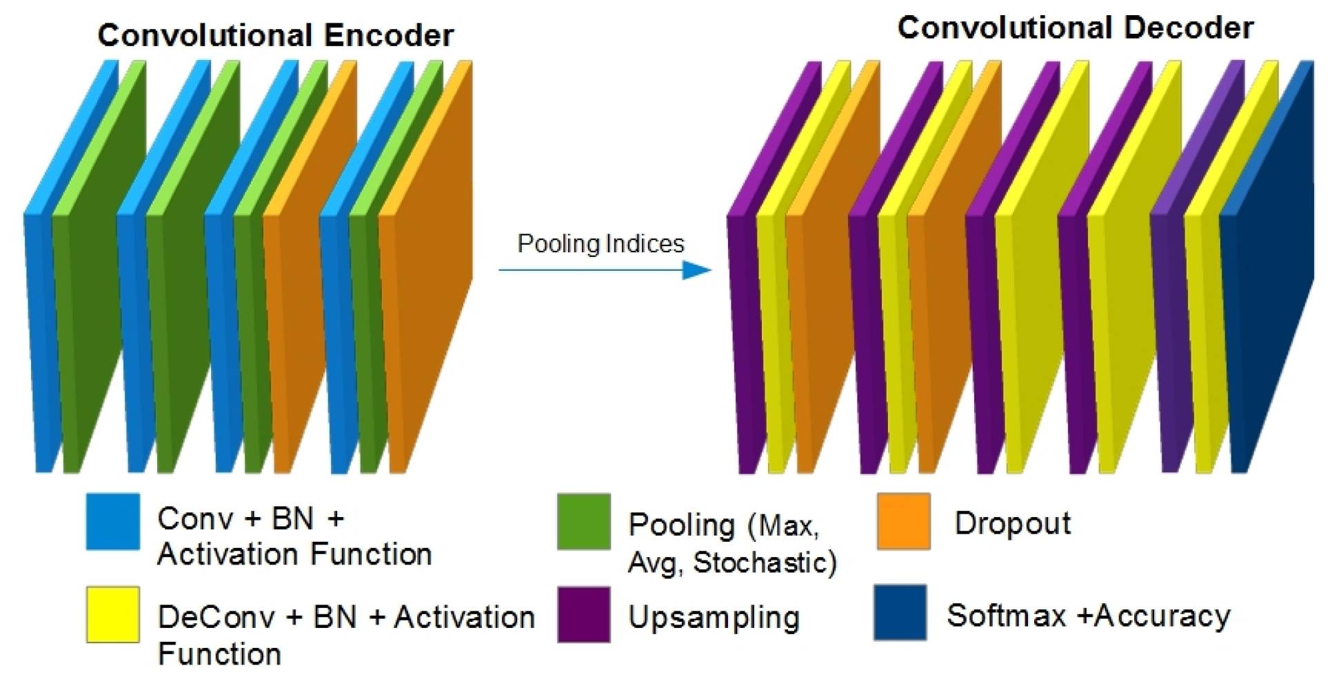
4. CSSA Architecture
To devise an enhanced and improved architecture, we have initially proposed a smaller version of the original network. This small version is a complete working model with a reduced number of layers. The idea is to perform experiments on the reduced version and to transfer high performance units (pooling methods, activation techniques) to the extended version. Figure 1 shows the initial base model (reduced version) of the proposed architecture. It is named the Basic Testing CNN Model (BTCM). It is based on encoder-decoder networks, which are presented separately with an image input and a corresponding image output with pixel-wise semantic segmentation.
The proposed architecture is a pixel-wise semantic segmentation engine, which is based on two decoupled encoding and decoding FCNs. The aforementioned encoder is based on the initial 13 convolution layers of the VGG-16 [47] network followed by the batch normalized [46] layer, an activation function, the pooling layer and dropout [48] units. Each layer in the proposed CNN is represented by a triplet , where I is a set of tensors, and each element I = is the input tensor for the l-th layer of CNN. W represents the set of tensors, where each element in this set W = is the k-th weight filter in the l-th CNN layer. Additionally, is the number of weight filters in the l-th layer of the proposed CNN. Here, * represents a convolutional operation with its operands and , where ∈ in which c, and represent channels, width and height, respectively. ∈ , where and . The decoder network is based on up-sampling layers, de-convolution layers, activation functions, batch normalized layers, dropout layers and a multi-class soft-max classifier layer. The whole architecture is based on an encoder-decoder relation where every decoder corresponds to a pooling unit of the encoder. Thus, the decoder CNN possesses 13 de-convolution layers. The decoder feeds its computations to a multi-class soft-max classifier to output the class probabilities intended for every pixel independently.
The network starts its training with an input image and proceeds through the network to final layers. The encoder performs convolution with a set filter banks to yield feature maps, and then, the batch normalization operation is performed. Later, Exponential Linear Units (ELU) [49] carry out activations. Then, the max-pooling operation is performed with a window size and stride-rate of two. In this way, the resultant image is sub-sampled by a factor of two. Whereas numerous pooling layers can offer more translation invariance for robust classification tasks, there is an unnecessary loss of spatial resolution of the feature maps. An image with increasingly lossy boundary details is not useful for segmentation tasks. Therefore, for semantic segmentation, boundary delineation is so important. Hence, there is a need for capturing and storing the boundary information in the encoder feature maps prior to the sub-sampling operation. However, due to memory constraints, it is not possible to store all encoder feature maps. The ultimate solution is to store only the max-pooling indices. The locations of every max-pooling feature-map are memorized using two bits for every pooling window. It is a very efficient solution to keep a large amount of feature maps. This solution offers a great deal of storage efficiency for the encoder, and we can get rid of the and layers.
Next, the decoder up-samples or un-pools the input feature map(s) in the decoder network. It utilizes the memorized max-pooling indices from the corresponding encoder’s feature map(s). This step generates sparse feature maps, which are later convolved with a trainable decoder filter bank to generate dense feature maps. The batch normalization is also applied over those maps. Finely, the high dimensional feature map(s) representation is fed to a trainable soft-max classifier that classifies every pixel independently. It outputs a K (number of classes) channel of image probabilities.
5. Experiments
5.1. Implementation Details
In order to test the performance of different CNN units, we initially tested a miniature version, i.e., BTCM. It is small, easy-to-train and convenient to change for different CNN’s units. It is inspired by SegNet-Basic and based on four encoder and decoder units. Each unit is composed of convolution layers, batch normalization layers, pooling layers and activation functions.
Test Model 1: The initial test was performed to choose the most appropriate activation function. For this purpose, we have tested the Tanh [50], Rectified Linear Unit (ReLU), Parametric Rectifier Linear Unit (PReLU) [45], Exponential Linear Units (ELU) [49] and Maxout [51]. We tried to assess the performance of all aforementioned activation functions on the proposed network and choose one with the best performance.
Test Model 2: The second test was performed to assess the best performing pooling method. We have tested the average, stochastic [52] and Max pooling methodologies. For this purpose, we trained the network with each of these pooling methods one-by-one and obtained the better performing units.
Test Model 3: The next experiment was performed to train the network without Batch Normalization (BN) layers. The key idea was to reduce the number of trainable parameters and the training time for the overall network. According to Schilling [53], batch normalization adds a certain amount of computational complexity that results in slightly higher training time. It is also assessed that batch normalization adds relatively more overhead by increasing the batch size. Therefore, we intend to train the network with less complexity and training time.
Test Model 4: Another experiment is performed to take out all pooling layers and the training network only with convolution layers. This idea is inspired by Springenberg et al. [54]. It is proposed that the pooling layer could be replaced with a normal convolution layer with a stride larger than one (i.e., for a pooling layer with and , it would be replaced with a convolution layer with a simpler stride rate and kernel size, where the number of output channels will be equal to the number of input channels). This experiment increases the number of trainable parameters, though the resultant network is much simplified as compared to the traditional CNN pipeline.
The procedure of replacing the pooling layers from the CNN network with standard convolutional layers having a higher stride rate can be explained by the standard formulation of defining convolution and pooling operations in CNNs. For example, f signifies a feature map produced by a particular layer of a CNN. It can be shown as a three-dimensional array of size, where W and H are the height and width, respectively, whereas N is the amount of given channels (in the case when f is the result of a convolutional layer, N is the amount of filters in this convolution layer) [54]. Then, p-norm subsampling (or pooling) having a pooling dimension k (or half-length ) and stride of r is implemented on the given feature map f with a three-dimensional array represented by the following entries:
where is a function mapping from positions in s to positions in f with stride rate r and p denotes the order of p-norm (for , it turns out to be the commonly-employed max pooling). If and pooling regions do not overlap, the present CNN network normally consists of an overlapping pooling by and .
The pooling operation stated in Equation (1) could be compared with the standard definition of a convolutional layer c applied to feature map f given as in Equation (3):
where is the convolutional layer weight (or the kernel weight, or the filter), is the activation function, is an activation function and is the amount of output features (or channels) of the convolutional layer. Through this analysis, it can be seen clearly that both operations rely on the similar elements of the previous network layer’s feature map [55]. The pooling layer could also be seen as a feature-wise convolution (where if u equals o and zero otherwise) in which we can replace the activation function with the p-norm. It is a perplexing question of whether and why such kinds of layers could be introduced. According to Springenberg et al. [54], the pooling layers contribute to the CNN architecture as follows: (1) the p-norm facilitates the network representation in a more invariant way; (2) the pooling layer’s spatial dimensionality reduction feature offers covering for large parts of the input image in higher layers; (3) the pooling layer’s feature-wise operation nature could help in making optimization easier as opposed to the convolutional layer operation where features get mixed. By taking the second point into consideration, the pooling layer dimensionality reduction is crucial for achieving good performance. Thus, this is a key hypothesis that we are going to test in this experiment.
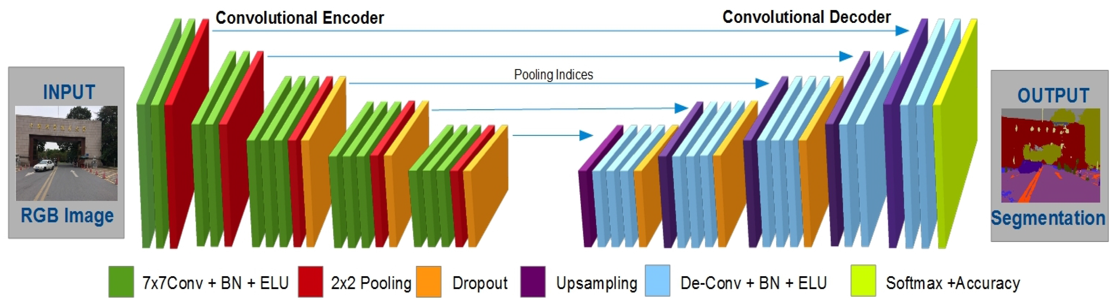
Test Model 5: After the deep and detailed analysis of different BTCMs, final tests will be conducted over the final version of our proposed network that will incorporate all best-performing components of the BTCM tests. Later, this model will be trained, and final assessments will be presented in the Results section. The illustration of the proposed CSSA architecture in shown in Figure 2. Apart from some differences, the proposed final model shares a similar architecture to a deconvolution network [15] and SegNet [40]. The deconvolution network by Noh et al. is based on 13 complete layers of VGG-16, which introduces much larger parameterization that leads to more computational resources. It is also difficult to train it end-to-end because of keeping the and layers, which leads to a huge number of trainable parameters to the decoder of the network. The CSSA proposed encoder excludes the and layers, which leads to less trainable parameters for the decoder. In this way, the proposed decoder needs less space and computational resources. SegNet is based on the ReLU activation function with no dropout units. ReLU is fast, non-saturating and shows very impressive results. However, in some situations, where it is not possible for ReLUs to saturate, it will turn units “dead” consequently. Moreover, they will never be activated because of the negative pre-activation value. In this situation, no gradient will flow through the network. Furthermore, ReLU is always non-negative; this means activation is always positive. The solution is ELU [49]; for positive values, it acts like ReLU, but in the case of negative values, it is a function bounded by a fixed value . In this way, it helps to push the neuron’s mean-activation closer to zero. It is quite beneficial for learning, and it facilitates learning for representations, which are more robust to noise. As a result, our proposed network will attain better speed-up learning via avoiding a bias shift. Furthermore, Srivastava et al. [48] proposed dropout units that will offer us a reduced chance of overfitting to the training data in comparison to SegNet. In fact, the proposed network will become less sensitive to the specific neuron’s weights. Consequently, the network will be able to better generalize and less likely to be overfitted.
The proposed final version for segmentation network is initiated with a class-specific activation map with a given input image . The input image is extracted from input layers and processed by convolution and pooling layers. Finally, from the decoder unit, it is passed to the class-specific segmentation map after applying the softmax function (where is the model parameter of the segmentation network). Here, has a background and foreground channels, which are denoted by and , respectively. Later, the segmentation job is formulated as the per-pixel regression to the ground-truth segmentation, which minimizes:
where is taken as the binary ground-truth segmentation mask for category l of the i-th image and is the segmentation loss of , or equivalently, the segmentation loss of , with respect to .
A channel-shared variant is considered as , where the coefficient is shared by all processing channels of the specific layer. In this way, this variant simply introduces a single extra parameter into every layer [56].
5.2. Training
The Caffe Berkeley Vision library [57] is used to develop and train the whole network. Caffe offers a great deal of freedom to write network layers and train the network according to the proposed requirements. Therefore, the network is trained once it converges, and no significant reduction in training loss is observed. Finally, the overall results are assessed, analyzed and later compared to the established benchmark results.
5.2.1. Datasets
We have used two well-known segmentation datasets (CamVid, PASCAL VOC-12) for overall experimentation. The aforementioned CamVid [37] dataset is used for overall training and testing of the proposed CNN architecture. It is composed of road scenes (day and dusk scenes) RGB images of a resolution. Our proposed network is designed to classify and segment 11 classes (e.g., cars, people, roads, buildings, poles, signs, trees, etc.). Local contrast normalization [58] is performed for each input image prior to training the network. There are testing, training and validation datasets for the overall CNN assessment.
The PASCAL VOC-12 segmentation dataset [7] is also employed for overall CNN training and testing. Pascal VOC-12 is an RGB dataset for segmentation. It contains training and validation images of indoor and outdoor scenes. The total number of images is 12,031. In the overall experimentation with CSSA, images are scaled to resolution for training and testing.
5.2.2. Optimization
All proposed CNN models are developed, trained and tested through the Berkeley-Vision deep learning framework Caffe. The proposed network is trained on a single NVIDIA Tesla K40c GPU with 12 G of memory. Training for reduced BTCM models takes approximately six hours. The training of network is performed until the loss is converged, and there is no considerable increase or decrease in loss and accuracy.
He et al.’s [45] proposed method for network initialization is used for the proposed encoder-decoder networks. Stochastic Gradient Descent (SGD) with the momentum of is employed to initiate the training of network. The network is trained with a fixed learning rate of [19], while the weight decay is . BTCM is trained for 10,000 iterations. Whereas the CSSA network is fixed to train no more than 40,000 iterations, as this limit is set to ensure that the network is trained enough and training loss is converging. To avoid the memory overflow problems while training, the training batch is set to 12 images. In each epoch, the image set is shuffled to ensure that no image is used more than once in any epoch.
The cross-entropy loss [59] is employed as the objective function for training the whole network. It sums up the overall loss of the pixels in a mini-batch and helps to assess the final loss.
6. Results and Analysis
This section will present the overall assessment for trained models and testing results by well-known segmentation and classification performance training measures, such as Global Accuracy (GA) and Class Average Accuracy (CAA). The GA offers an overall percentage of pixels properly classified in the dataset, while CAA is used to assess the predictive accuracy mean of the entire classes. Proposed tests were performed on BTCM with comparatively less training iterations. The proposed network is limited to run for a maximum of 10,000 training transactions to test the ultimate reduction in loss and enhancement in accuracy; whereas the final version of the proposed CNN is trained for 40,000 iterations.
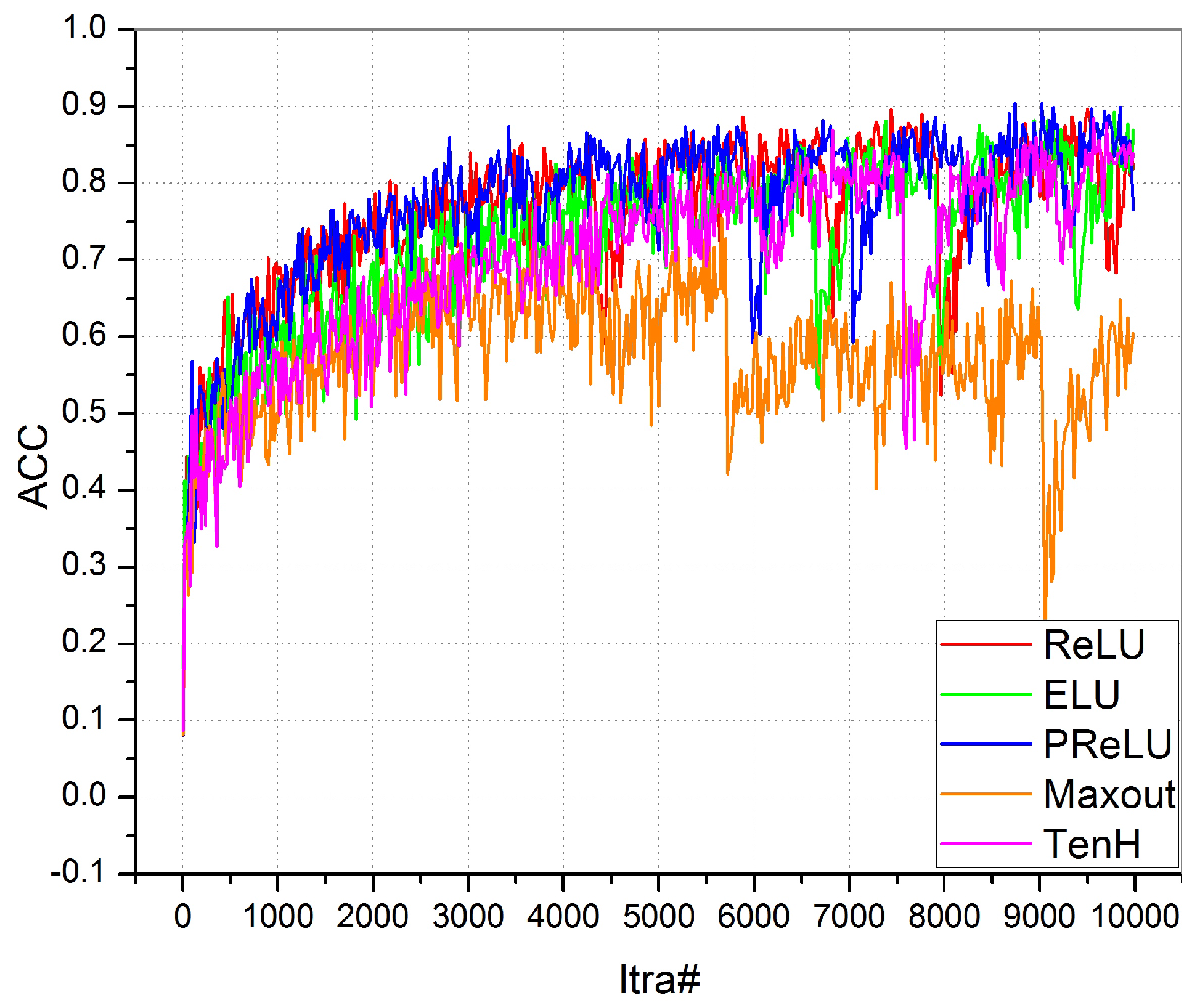
Test 1: Different kinds of tests are performed on BTCM. The proposed model is used for the training efficiency of different activation functions. We have tested for ReLU, ELU, PReLU, Maxout and Tanh. The final outcomes showed that ELU and PReLU are performing better and offer enhanced outcomes. It is assessed that the PReLU performs well throughout the training process, but accuracy declines at the end of the training process, as shown in Figure 3. The ELU converged to the ultimate peak till the end of the training process.
The Exponential Linear Unit (ELU) with is:
The ELU hyperparameter manages the given value to which an ELU saturates for negative net-inputs. ELUs reduce the chances of vanishing gradient effect as Leaky ReLUs (LReLUs) and ReLUs do. The problem of the vanishing gradient is eased because the positive part of these functions is the identity; hence, their derivative is one and not contractive. However, sigmoid and tanh activation functions are contractive nearly everywhere. Contrary to ReLUs, ELUs offer negative values, which can push the mean of the activations very near to zero. The closer to zero, the faster the learning by the activation function, as this brings the gradient closer to the natural gradient. ELUs saturate to a negative value when the argument value gets smaller. Saturation means a small derivative that decreases the variation, as well as the information that is transferred to the next layer. Consequently, the representation is both of low-complexity and noise-robust.
Test 2: In Test 2, the BTCM is tested for different pooling techniques (average, max and stochastic). The final outcomes have shown that the max pooling method is outperforming all existing methods. Figure 4 shows that the max pooling training accuracy is converging quickly as compared to other methods. The CSSA final version will be trained with the max pooling units.
Test 3: Batch normalization layers offer us a higher accuracy and faster learning at the expense of additional computations and trainable parameters. This leads the learning process to become slower. To assess network performance and train it in a faster way, we have removed BN layers and try to train the network; though, the outcomes are not really encouraging. Figure 5 shows the final outcomes of the proposed model. The initial loss is too high, and it reduces down too slowly; whereas, the accuracy is improving slowly, and there is no considerable increase in it after a number of training iterations. According to Schilling [53], besides a certain amount of computational complexity, there are out-weighed benefits attained by introducing the batch normalization unit. It is further mentioned that by reducing the batch size, we can efficiently reduce the batch normalization-associated overheads. It can also be achieved by sparsely distributing normalization layers throughout the CNN architecture. Therefore, the final version of CSSA is trained with sparse BN layers and a small batch size. We set the batch size limit to 12 to avoid BN-associated overheads.
Test 4: To simplify the CNN pipeline, we propose Springenberg et al.’s [54] inspired BTCM and train it. The results are shown in Figure 6. It shows a very poor training outcome, where the accuracy remains close to zero, and loss stays higher than one. The outcomes are really discouraging, so this BTCM design is discarded from further analysis. The hypothesis to eliminate the pooling layer for the sake of network simplicity is not successful due to the whole network getting degraded through consecutive convolutions. Therefore, for the final CSSA experimentation, we eliminate the current BTCM and continue with max pooling units.
Test 5: The CSSA is a VGG-16-based model. Its architecture is shown in Table 1. It is composed of the best performing ELU activation function, the max pooling unit and BN layer. The aforementioned whole network is based on an encoder-decoder arrangement, which is trained end-to-end over the Pascal VOC-12 and CamVid datasets.
The final results are assessed with benchmark results, and it is noticed that the proposed network out-performer with an improved ELU activation function and other units. Figure 7 shows the accuracy vs. loss comparison of our proposed network. The “x-axis” shows the number of training iterations, while the “y-axis” shows the training accuracy and loss. We set a low learning rate that helps us to reduce training loss very slowly. After analyzing the curves, it can be claimed that our proposed network achieves a good learning rate, as the “red” accuracy curve moves smoothly, and finally, it attains the best performance. A similar smoothness is achieved with the “green” loss curve. It can be observed that the loss is gradually decreasing and accuracy is improving alongside, until they become constant. It is the ultimate performance of the CSSA network. “A” is the proposed network, while “B” is SegNet, which is used as the benchmark result for analysis. It can be clearly observed that the proposed network is performing well with perfect converging loss and accuracy curves as compared to its counterpart.
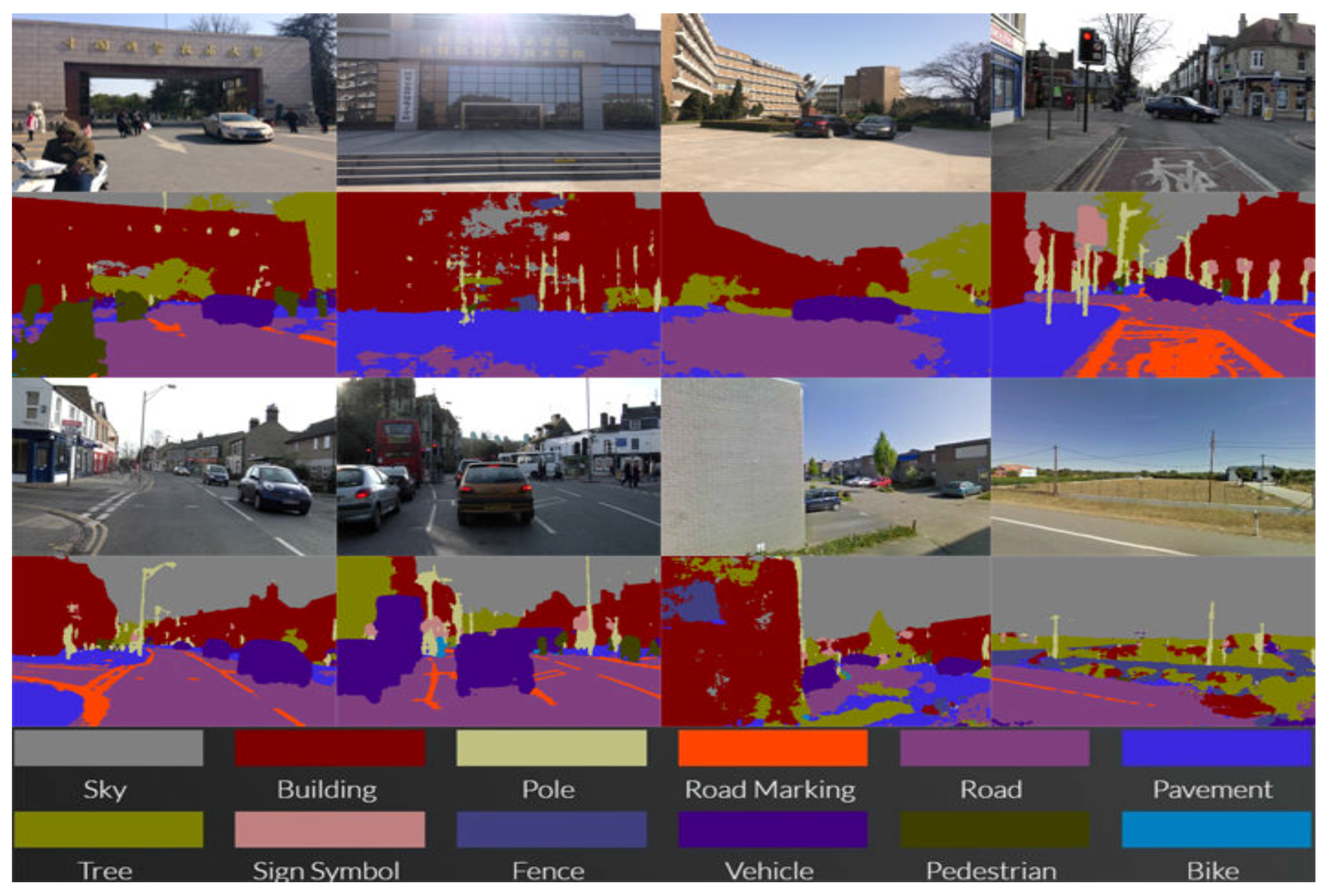
Figure 8 shows different road-scene training and testing set images and their corresponding results. The resultant images show clear boundary delineation among different object. It also shows a significantly efficient result regarding the detection of objects in a given image.
Table 2 shows quantitative results on the CamVid dataset. Our proposed CSSA results are compared with other popular benchmark results. The road scene detection process comprises 11 road scene categories. The proposed CSSA outperforms over all other methods. There is a great deal of improvement in class average accuracy and global accuracy for the smaller classes.
The Pascal VOC-12 [7] segmentation dataset is composed of the segmentation of a few salient object classes with usually a variable background class. It is different from earlier segmentation for road scene understanding benchmarks, which need to learn both classes and their spatial context. Table 3 presents the Pascal VOC-12 segmentation challenge results in comparison with established benchmark results. The proposed CSSA is intended for road scene understanding; therefore, we do not intend to benchmark this experiment to attain the top rank in the Pascal VOC-12 segmentation challenge. Therefore, the CSSA is not trained by using multi-stage training [17] or post-processing, which uses CRF-based methods [15,16]. The CSSA network is trained end-to-end without any other assistance, and Table 3 presents the resultant performance. Early best-performing benchmark networks are either very large [15] and/or they use a CRF (such as [66] use Recurrent Neural Networks (RNNs)). In contrast, the key object behind CSSA implementation is to reduce the number of trainable parameters and improve overall inference time without other aids. We have reported results in terms of class average accuracy and the size of the network.
There is little loss recorded in the performance due to dropping fully-connected layers. However, this reduces the size of CSSA and offers us the capability to train the network end-to-end. Although it may be argued that bigger and denser CNNs can have outstanding performance, it is at the cost of increased memory requirements and longer inference time. This kind of architecture also leads to a complex training mechanism. Due to such kinds of bottlenecks, bigger and denser CNNs are not appropriate for real-time applications, such as road scene understanding. Therefore, the CSSA could be a preferred choice for the ADAS architecture.
According to a report by [67], during 1990–2010, 54 million people were injured in roadside accidents. About 1.4 million deaths occurred since 2013, and in 68,000 cases, the victims were children less than five years old. In all of these cases, 93 percent of crashes were due to driver error/ human factors. Thus, to avoid such situations, there is a new technology-based ADAS solution, which is the ultimate choice. Since the initiation of the autonomous vehicles grand challenges by DARPA [68], there has been an explosion in research for designing and developing of driving assistance systems. A number of automakers have initiated vehicle ADAS to mitigate driver stress and fatigue to offer additional safety features. However, self-driving cars are over promised and under delivered so far. Society of Automotive Engineers (SAE) [69] has proposed five levels of vehicle automation in which we still stand on Level 3. The key reason is the lack of efficient technology and expensive solutions. These days, headway sensors (short range and long radars) are used in cars for ADAS. However, these solutions are expensive and prone to some of road conditions (corners, narrow turns, etc.). However, some vision-based applications, such as the “German Traffic Sign Recognition System” by Stallkamp et al. [70], have attained 99 percent accuracy. These kinds of achievements had opened new horizons for vision-based applications for road scene understanding and ADAS. From traffic sign detection [71] to pedestrian detection [72], CNNs are offering a great deal of support and capability to attain the SAE five-level goals in the near future. The proposed CSSA is a small step toward achieving this great goal. It offers a higher accuracy rate for 11 road objects. This CNN could be trained and transformed according to any image size and requirements. It is a low cost and efficient solution for ADAS, will offer a more efficient performance and could be adopted as the video component for the ADAS toolkit. To enhance the potential performance of the proposed system, a larger road scene dataset is needed. By using existing sensors, such as mm-accurate GPS and LiDAR [44], and calibrating them with cameras, a more comprehensive video dataset could be created. This dataset will contain the labeled lane-markings and annotated vehicles with location and relative speed. In this way, a labeled dataset with diverse driving situations (snow, rain, day, night, etc.) could be created. Training the proposed CNN on such a dataset would offer a robust ADAS support system.
7. Conclusions
This research has offered a novel model of CNN with more enhanced and tested units. This proposed FCN model is offering high performance and better results in comparison to the established benchmarks’ results. The proposed system is a semantic pixel-wise segmentation engine. It offers a unique combination of encoder-decoder networks working together to offer an enhanced performance and improved outcomes. In this research, we have experimented with a miniature version of the proposed model and, later, transferred the outperforming units and layers to a larger CSSA architecture. It has offered us a great deal of efficiency to train and test networks in less time. The final CSSA model has performed efficiently and offered outstanding results in comparison with earlier similar approaches. Nowadays, ultrasonic and a few other types of radars are used in smart automobiles. The ADAS requires such radars and other technologies that can be applicable in all types of road and weather conditions. Using the CNN-based road scene detection and understating system in the automobile, it will be helpful especially in odd road conditions and blind spots where ultrasonic signals are unable to identify objects. In the future, we intend to improve the performance of the proposed network by developing and designing a time and space efficient binarized neural network for road scene understanding. It will be a much faster and efficient architecture to facilitate real-time decision making for the road scene understanding scenario.
Acknowledgments
This research is supported by Chinese Academy of Sciences (CAS) and The World Academy of Sciences (TWAS)’s President PhD Fellowship Programme and the University of Science and Technology of China, Hefei, China. We pay special gratitude to our colleagues who provided insight and expertise that greatly assisted this research work.
Author Contributions
Robail Yasrab conceived and wrote the paper; Xiaoci Zhang helped in experiments; Naijie Gu offered useful suggestions for developing algorithms and writing the paper.
Conflicts of Interest
The authors declare no conflict of interest.
Abbreviations
The following abbreviations are used in this manuscript:
| ADAS | Advanced Driver Assistance System |
| CNN | Convolution Neural Network |
| CSSA | CNN for Semantic Segmentation for ADAS |
| BN | Batch Normalization |
| FCN | Fully-Convolutional Networks |
| ReLU | Rectified Linear Unit |
| RNN | Recurrent Neural Network |
| LReLU | Leaky ReLUs |
References
- Hinton, G.; Deng, L.; Yu, D.; Dahl, G.E.; Mohamed, A.R.; Jaitly, N.; Senior, A.; Vanhoucke, V.; Nguyen, P.; Sainath, T.N.; et al. Deep neural networks for acoustic modeling in speech recognition: The shared views of four research groups. IEEE Signal Proc. Mag. 2012, 29, 82–97. [Google Scholar] [CrossRef]
- Krizhevsky, A.; Sutskever, I.; Hinton, G.E. Imagenet classification with deep convolutional neural networks. In Advances in Neural Information Processing Systems; Curran Associates Inc.: Red Hook, NY, USA, 2012; pp. 1097–1105. [Google Scholar]
- Szegedy, C.; Liu, W.; Jia, Y.; Sermanet, P.; Reed, S.; Anguelov, D.; Erhan, D.; Vanhoucke, V.; Rabinovich, A. Going deeper with convolutions. In Proceedings of the IEEE Conference on Computer Vision and Pattern Recognition, Boston, MA, USA, 7–12 June 2015; pp. 1–9. [Google Scholar]
- Desai, P.R.; Desai, P.N.; Ajmera, K.D.; Mehta, K. A review paper on oculus rift-a virtual reality headset. arXiv, 2014; arXiv:1408.1173. [Google Scholar]
- Gottmer, M. Merging Reality and Virtuality with Microsoft HoloLens. Master’s Thesis, Universiteit Utrecht, Utrecht, The Netherlands, 2015. [Google Scholar]
- Shotton, J.; Sharp, T.; Kipman, A.; Fitzgibbon, A.; Finocchio, M.; Blake, A.; Cook, M.; Moore, R. Real-time human pose recognition in parts from single depth images. Commun. ACM 2013, 56, 116–124. [Google Scholar] [CrossRef]
- Everingham, M.; Van Gool, L.; Williams, C.K.; Winn, J.; Zisserman, A. The pascal visual object classes (voc) challenge. Int. J. Comput. Vis. 2010, 88, 303–338. [Google Scholar] [CrossRef]
- Couprie, C.; Farabet, C.; Najman, L.; LeCun, Y. Indoor semantic segmentation using depth information. arXiv, 2013; arXiv:1301.3572. [Google Scholar]
- Donahue, J.; Jia, Y.; Vinyals, O.; Hoffman, J.; Zhang, N.; Tzeng, E.; Darrell, T. DeCAF: A Deep Convolutional Activation Feature for Generic Visual Recognition. arXiv, 2014; 647–655arXiv:1310.1531. [Google Scholar]
- Hariharan, B.; Arbeláez, P.; Girshick, R.; Malik, J. Simultaneous detection and segmentation. In European Conference on Computer Vision; Springer: Zurich, Switzerland, 2014; pp. 297–312. [Google Scholar]
- Ciresan, D.; Giusti, A.; Gambardella, L.M.; Schmidhuber, J. Deep neural networks segment neuronal membranes in electron microscopy images. In Advances in Neural Information Processing Systems; Curran Associates, Inc.: Red Hook, NY, USA, 2012; pp. 2843–2851. [Google Scholar]
- Farabet, C.; Couprie, C.; Najman, L.; LeCun, Y. Learning hierarchical features for scene labeling. IEEE Trans. Pattern Anal. Mach. Intell. 2013, 35, 1915–1929. [Google Scholar] [CrossRef] [PubMed]
- Ravì, D.; Bober, M.; Farinella, G.M.; Guarnera, M.; Battiato, S. Semantic segmentation of images exploiting DCT based features and random forest. Pattern Recognit. 2016, 52, 260–273. [Google Scholar] [CrossRef]
- Visin, F.; Ciccone, M.; Romero, A.; Kastner, K.; Cho, K.; Bengio, Y.; Matteucci, M.; Courville, A. Reseg: A recurrent neural network-based model for semantic segmentation. In Proceedings of the IEEE Conference on Computer Vision and Pattern Recognition Workshops, Seattle, WA, USA, 27–30 June 2016; pp. 41–48. [Google Scholar]
- Noh, H.; Hong, S.; Han, B. Learning deconvolution network for semantic segmentation. In Proceedings of the IEEE International Conference on Computer Vision, Santiago, Chile, 7–13 December 2015; pp. 1520–1528. [Google Scholar]
- Chen, L.C.; Papandreou, G.; Kokkinos, I.; Murphy, K.; Yuille, A.L. Semantic image segmentation with deep convolutional nets and fully connected crfs. arXiv, 2014; arXiv:1412.7062. [Google Scholar]
- Long, J.; Shelhamer, E.; Darrell, T. Fully convolutional networks for semantic segmentation. In Proceedings of the IEEE Conference on Computer Vision and Pattern Recognition, Boston, MA, USA, 7–12 June 2015; pp. 3431–3440. [Google Scholar]
- Shotton, J.; Winn, J.; Rother, C.; Criminisi, A. Textonboost for image understanding: Multi-class object recognition and segmentation by jointly modeling texture, layout, and context. Int. J. Comput. Vis. 2009, 81, 2–23. [Google Scholar] [CrossRef]
- Bottou, L. Large-scale machine learning with stochastic gradient descent. Proceedings of COMPSTAT’2010; Springer: Paris, France, 2010; pp. 177–186. [Google Scholar]
- Al Machot, F.; Ali, M.; Haj Mosa, A.; SchwarzlmxFC;ller, C.; Gutmann, M.; Kyamakya, K. Real-time raindrop detection based on cellular neural networks for ADAS. J. Real-Time Image Proc. 2016, 1–13. [Google Scholar] [CrossRef]
- Girshick, R.; Donahue, J.; Darrell, T.; Malik, J. Rich feature hierarchies for accurate object detection and semantic segmentation. In Proceedings of the IEEE Conference on Computer Vision and Pattern Recognition, Columbus, OH, USA, 23–28 June 2014; pp. 580–587. [Google Scholar]
- Zbontar, J.; LeCun, Y. Computing the stereo matching cost with a convolutional neural network. In Proceedings of the IEEE Conference on Computer Vision and Pattern Recognition, Boston, MA, USA, 7–12 June 2015; pp. 1592–1599. [Google Scholar]
- Tompson, J.J.; Jain, A.; LeCun, Y.; Bregler, C. Joint training of a convolutional network and a graphical model for human pose estimation. In Advances in Neural Information Processing Systems; NIPS: Montreal, QC, Canada, 2014; pp. 1799–1807. [Google Scholar]
- Gupta, S.; Girshick, R.; Arbeláez, P.; Malik, J. Learning rich features from RGB-D images for object detection and segmentation. In European Conference on Computer Vision; Springer: Zurich, Switzerland, 2014; pp. 345–360. [Google Scholar]
- Guo, X.; Shen, C.; Chen, L. Deep Fault Recognizer: An Integrated Model to Denoise and Extract Features for Fault Diagnosis in Rotating Machinery. Appl. Sci. 2016, 7, 41. [Google Scholar] [CrossRef]
- Wang, J.; Zhang, G.; Shi, J. 2D Gaze Estimation Based on Pupil-Glint Vector Using an Artificial Neural Network. Appl. Sci. 2016, 6, 174. [Google Scholar] [CrossRef]
- LeCun, Y.; Boser, B.; Denker, J.S.; Henderson, D.; Howard, R.E.; Hubbard, W.; Jackel, L.D. Backpropagation applied to handwritten zip code recognition. Neural Comput. 1989, 1, 541–551. [Google Scholar] [CrossRef]
- Matan, O.; Burges, C.J.; LeCun, Y.; Denker, J.S. Multi-Digit Recognition Using a Space Displacement Neural Network; NIPS: San Mateo, CA, USA, 1991; pp. 488–495. [Google Scholar]
- Wolf, R.; Platt, J.C. Postal address block location using a convolutional locator network. In Advances in Neural Information Processing Systems; NIPS: Denver, CO, USA, 1994; p. 745. [Google Scholar]
- Ning, F.; Delhomme, D.; LeCun, Y.; Piano, F.; Bottou, L.; Barbano, P.E. Toward automatic phenotyping of developing embryos from videos. IEEE Trans. Image Proc. 2005, 14, 1360–1371. [Google Scholar] [CrossRef]
- Koltun, V. Efficient inference in fully connected crfs with gaussian edge potentials. Adv. Neural Inf. Process. Syst. 2011, 2, 1–9. [Google Scholar]
- Mostajabi, M.; Yadollahpour, P.; Shakhnarovich, G. Feedforward semantic segmentation with zoom-out features. In Proceedings of the IEEE Conference on Computer Vision and Pattern Recognition, Boston, MA, USA, 7–12 June 2015; pp. 3376–3385. [Google Scholar]
- Dai, J.; He, K.; Sun, J. Convolutional feature masking for joint object and stuff segmentation. In Proceedings of the IEEE Conference on Computer Vision and Pattern Recognition, Boston, MA, USA, 7–12 June 2015; pp. 3992–4000. [Google Scholar]
- Hariharan, B.; Arbeláez, P.; Girshick, R.; Malik, J. Hypercolumns for object segmentation and fine-grained localization. In Proceedings of the IEEE Conference on Computer Vision and Pattern Recognition, Boston, MA, USA, 7–12 June 2015; pp. 447–456. [Google Scholar]
- Shotton, J.; Johnson, M.; Cipolla, R. Semantic texton forests for image categorization and segmentation. In Proceedings of the IEEE Conference on Computer Vision and Pattern Recognition, Anchorage, KY, USA, 23–28 June 2008; pp. 1–8. [Google Scholar]
- Sturgess, P.; Alahari, K.; Ladicky, L.; Torr, P.H. Combining appearance and structure from motion features for road scene understanding. In Proceedings of the BMVC 2012-23rd British Machine Vision Conference, London, UK, 7–10 September 2009. [Google Scholar]
- Brostow, G.J.; Fauqueur, J.; Cipolla, R. Semantic object classes in video: A high-definition ground truth database. Pattern Recognit. Lett. 2009, 30, 88–97. [Google Scholar] [CrossRef]
- Ladickỳ, L.; Sturgess, P.; Alahari, K.; Russell, C.; Torr, P.H. What, where and how many? Combining object detectors and crfs. In European Conference on Computer Vision; Springer: Crete, Greece, 2010; pp. 424–437. [Google Scholar]
- Huang, F.J.; Boureau, Y.L.; LeCun, Y. Unsupervised learning of invariant feature hierarchies with applications to object recognition. In Proceedings of the 2007 IEEE Conference on Computer Vision and Pattern Recognition, Minneapolis, MN, USA, 18–23 June 2007; pp. 1–8. [Google Scholar]
- Badrinarayanan, V.; Handa, A.; Cipolla, R. Segnet: A deep convolutional encoder-decoder architecture for robust semantic pixel-wise labelling. arXiv, 2015; arXiv:1505.07293. [Google Scholar]
- Kendall, A.; Badrinarayanan, V.; Cipolla, R. Bayesian segnet: Model uncertainty in deep convolutional encoder-decoder architectures for scene understandingBayesian segnet. arXiv, 2015; arXiv:1511.02680. [Google Scholar]
- Jung, H.; Choi, M.K.; Soon, K.; Jung, W.Y. End-to-End Pedestrian Collision Warning System based on a Convolutional Neural Network with Semantic Segmentation. arXiv, 2016; arXiv arXiv:1612.06558. [Google Scholar]
- Xie, K.; Ge, S.; Ye, Q.; Luo, Z. Traffic Sign Recognition Based on Attribute-Refinement Cascaded Convolutional Neural Networks. In Pacific Rim Conference on Multimedia; Springer: Xi’an, China, 2016; pp. 201–210. [Google Scholar]
- Huval, B.; Wang, T.; Tandon, S.; Kiske, J.; Song, W.; Pazhayampallil, J.; Andriluka, M.; Rajpurkar, P.; Migimatsu, T.; Cheng-Yue, R.; et al. An empirical evaluation of deep learning on highway driving. arXiv, 2015; arXiv:1504.01716. [Google Scholar]
- He, K.; Zhang, X.; Ren, S.; Sun, J. Delving deep into rectifiers: Surpassing human-level performance on imagenet classification. In Proceedings of the IEEE International Conference on Computer Vision, Santiago, Chile, 7–13 December 2015; pp. 1026–1034. [Google Scholar]
- Ioffe, S.; Szegedy, C. Batch normalization: Accelerating deep network training by reducing internal covariate shift. arXiv, 2015; arXiv:1502.03167. [Google Scholar]
- Simonyan, K.; Zisserman, A. Very deep convolutional networks for large-scale image recognition. arXiv, 2014; arXiv:1409.1556. [Google Scholar]
- Srivastava, N.; Hinton, G.E.; Krizhevsky, A.; Sutskever, I.; Salakhutdinov, R. Dropout: A simple way to prevent neural networks from overfitting. J. Mach. Learn. Res. 2014, 15, 1929–1958. [Google Scholar]
- Clevert, D.A.; Unterthiner, T.; Hochreiter, S. Fast and accurate deep network learning by exponential linear units (elus). arXiv, 2015; arXiv:1511.07289. [Google Scholar]
- Drucker, H.; Le Cun, Y. Improving generalization performance in character recognition. In Proceedings of the 1991 IEEE Workshop on Neural Networks for Signal Processing, New York, NY, USA, 30 September–1 October 1991; pp. 198–207. [Google Scholar]
- Goodfellow, I.J.; Warde-Farley, D.; Mirza, M.; Courville, A.C.; Bengio, Y. Maxout networks. ICML (3) 2013, 28, 1319–1327. [Google Scholar]
- Zeiler, M.D.; Fergus, R. Stochastic pooling for regularization of deep convolutional neural networks. arXiv, 2013; arXiv:1301.3557. [Google Scholar]
- Schilling, F. The Effect of Batch Normalization on Deep Convolutional Neural Networks; DiVA Publisher: Uppsala, Sweden, 2016. [Google Scholar]
- Springenberg, J.T.; Dosovitskiy, A.; Brox, T.; Riedmiller, M. Striving for simplicity: The all convolutional net. arXiv, 2014; arXiv:1412.6806. [Google Scholar]
- Yasrab, R.; GU, N.; Xiaoci, Z. SCNet: A Simplified Encoder-Decoder CNN for Semantic Segmentation. In Proceedings of the 2016 IEEE Sponsored 5th International Conference on Computer Science and Networks Technology (ICCSNT 2016), Changchun, China, 10–11 December 2016; pp. 1–6. [Google Scholar]
- Yasrab, R.; GU, N.; Xiaoci, Z.; Asad-Khan. DCSeg: Decoupled CNN for Classification and Semantic Segmentation. In Proceedings of the 2017 IEEE Conference on Knowledge and Smart Technologies (KST), Pattaya, Thailand, 1–4 February 2017; pp. 1–6. [Google Scholar]
- Jia, Y.; Shelhamer, E.; Donahue, J.; Karayev, S.; Long, J.; Girshick, R.; Guadarrama, S.; Darrell, T. Caffe: Convolutional architecture for fast feature embedding. In Proceedings of the 22nd ACM International Conference on Multimedia, Orlando, FL, USA, 3–7 November 2014; pp. 675–678. [Google Scholar]
- Jarrett, K.; Kavukcuoglu, K.; Lecun, Y. What is the best multi-stage architecture for object recognition? In Proceedings of the 2009 IEEE 12th International Conference on Computer Vision, Kyoto, Japan, 27 September–4 October 2009; pp. 2146–2153. [Google Scholar]
- Murphy, K.P. Machine Learning: A Probabilistic Perspective; MIT Press: Cambridge, MA, USA, 2012. [Google Scholar]
- Yang, Y.; Li, Z.; Zhang, L.; Murphy, C.; Ver Hoeve, J.; Jiang, H. Local label descriptor for example based semantic image labeling. In European Conference on Computer Vision; Springer: Zurich, Switzerland, 2012; pp. 361–375. [Google Scholar]
- Brostow, G.J.; Shotton, J.; Fauqueur, J.; Cipolla, R. Segmentation and recognition using structure from motion point clouds. In European Conference on Computer Vision; Springer: Marseille, France, 2008; pp. 44–57. [Google Scholar]
- Zhang, C.; Wang, L.; Yang, R. Semantic segmentation of urban scenes using dense depth maps. In European Conference on Computer Vision; Springer: Crete, Greece, 2010; pp. 708–721. [Google Scholar]
- Kontschieder, P.; Bulo, S.R.; Bischof, H.; Pelillo, M. Structured class-labels in random forests for semantic image labelling. In Proceedings of the 2011 IEEE International Conference on Computer Vision (ICCV), Barcelona, Spain, 6 November–13 November 2011; pp. 2190–2197. [Google Scholar]
- Rota Bulo, S.; Kontschieder, P. Neural decision forests for semantic image labelling. In Proceedings of the IEEE Conference on Computer Vision and Pattern Recognition, Columbus, IN, USA, 23–28 June 2014; pp. 81–88. [Google Scholar]
- Tighe, J.; Lazebnik, S. Superparsing. Int. J. Comput. Vis. 2013, 101, 329–349. [Google Scholar] [CrossRef]
- Zheng, S.; Jayasumana, S.; Romera-Paredes, B.; Vineet, V.; Su, Z.; Du, D.; Huang, C.; Torr, P.H. Conditional random fields as recurrent neural networks. In Proceedings of the IEEE International Conference on Computer Vision, Santiago, Chile, 7–13 December 2015; pp. 1529–1537. [Google Scholar]
- Lim, S.S.; Vos, T.; Flaxman, A.D.; Danaei, G.; Shibuya, K.; Adair-Rohani, H.; AlMazroa, M.A.; Amann, M.; Anderson, H.R.; Andrews, K.G.; et al. A comparative risk assessment of burden of disease and injury attributable to 67 risk factors and risk factor clusters in 21 regions, 1990–2010: A systematic analysis for the Global Burden of Disease Study 2010. Lancet 2013, 380, 2224–2260. [Google Scholar] [CrossRef]
- Thrun, S.; Montemerlo, M.; Dahlkamp, H.; Stavens, D.; Aron, A.; Diebel, J.; Fong, P.; Gale, J.; Halpenny, M.; Hoffmann, G.; et al. Stanley: The robot that won the DARPA Grand Challenge. J. Field Robot. 2006, 23, 661–692. [Google Scholar] [CrossRef]
- SAE, T. Definitions for Terms Related to On-Road Motor Vehicle Automated Driving Systems-J3016. In Society of Automotive Engineers: On-Road Automated Vehicle Standards Committee; SAE Pub. Inc.: Warrendale, PA, USA, 2013. [Google Scholar]
- Stallkamp, J.; Schlipsing, M.; Salmen, J.; Igel, C. The German traffic sign recognition benchmark: A multi-class classification competition. In Proceedings of the 2011 International Joint Conference on Neural Networks (IJCNN), San Jose, CA, USA, 31 July–5 August 2011; pp. 1453–1460. [Google Scholar]
- Lee, S.S.; Lee, E.; Hwang, Y.; Jang, S.J. Low-complexity hardware architecture of traffic sign recognition with IHSL color space for advanced driver assistance systems. In Proceedings of the IEEE International Conference on Consumer Electronics-Asia (ICCE-Asia), Nagoya, Japan, 24–27 October 2016; pp. 1–2. [Google Scholar]
- Sermanet, P.; Eigen, D.; Zhang, X.; Mathieu, M.; Fergus, R.; LeCun, Y. Overfeat: Integrated recognition, localization and detection using convolutional networks. arXiv, 2013; arXiv:1312.6229. [Google Scholar]
Figure 1.
Basic Testing CNN Model (BTCM).

Figure 2.
An illustration of the proposed CSSA architecture.

Figure 3.
Comparison of different activation functions.

Figure 4.
Pooling methods’ accuracy curves.
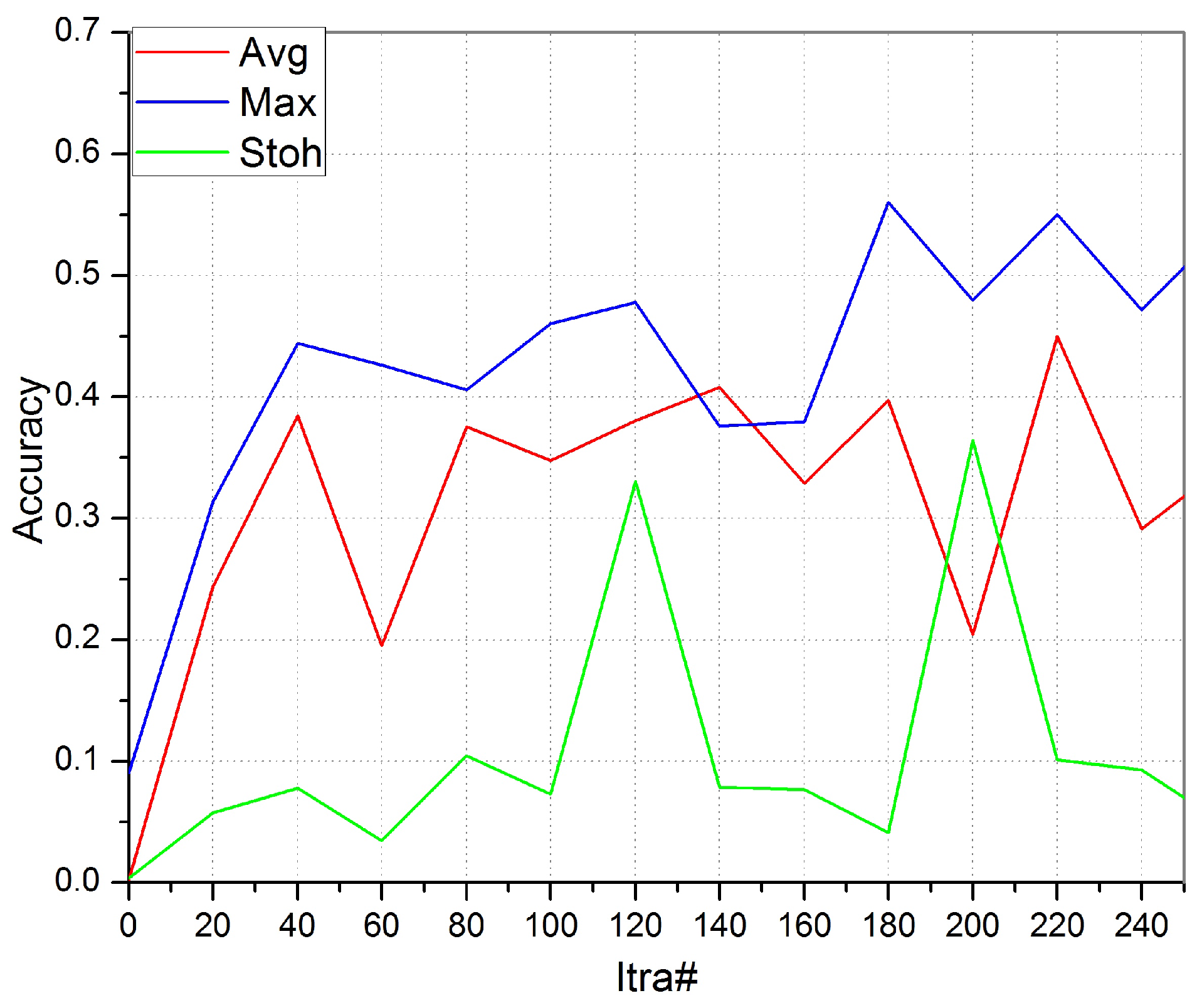
Figure 5.
CNN network results without Batch Normalization (BN) layers.

Figure 6.
Analysis of CNN by skipping pooling layers.
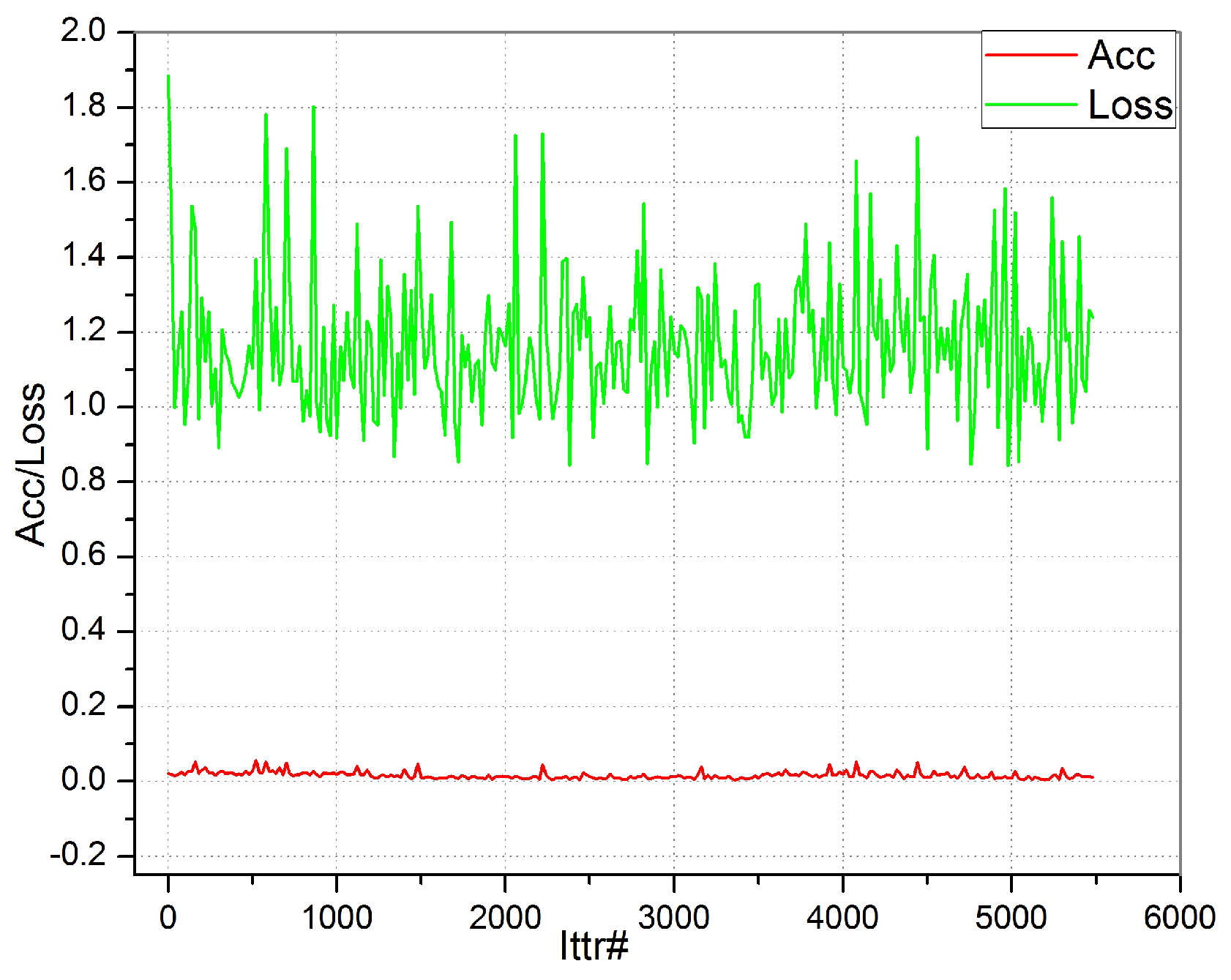
Figure 7.
CSSA vs. SegNet.
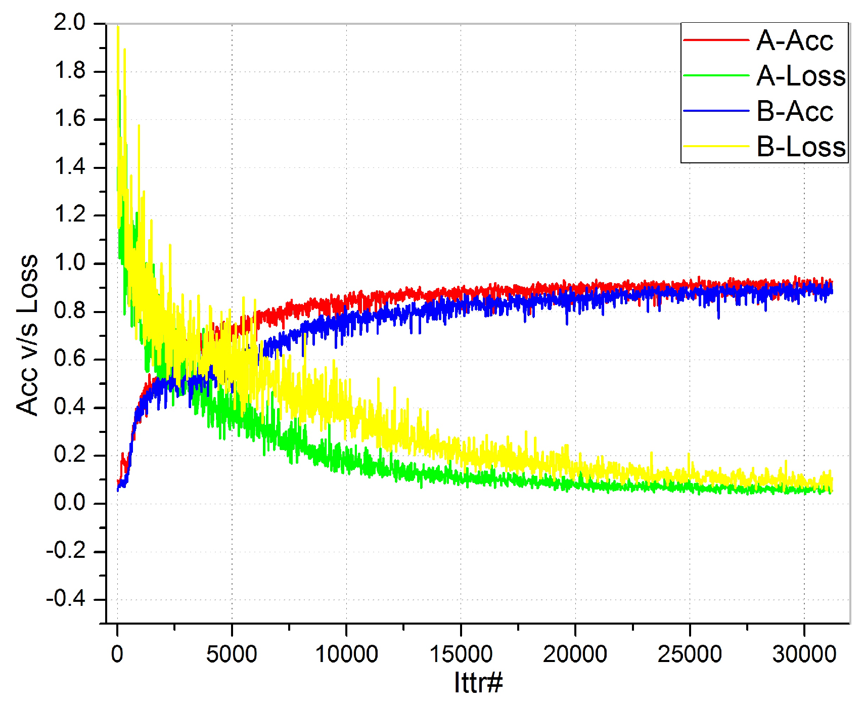
Figure 8.
CSSA image dataset results.

Table 1.
CSSA’s encoder and decoder layer architecture.
| Encoder | Decoder | ||||
|---|---|---|---|---|---|
| Input 360 × 480 + Norm | Output, Soft-max-with-Loss, Accuracy | ||||
| Conv1 | 3 × 3, 64 | BN, ELU, Pooling | De-Conv | 3 × 3, 64 | Up-sample, BN, ELU |
| 3 × 3, 64 | 3 × 3, 64 | ||||
| Conv2 | 3 × 3, 128 | BN, ELU, Pooling | De-Conv | 3 × 3, 128 | Up-sample, BN, ELU |
| 3 × 3, 128 | 3 × 3, 128 | ||||
| Conv3 | 3 × 3, 256 | BN, ELU, Pooling, Dropout | De-Conv | 3 × 3, 256 | Up-sample, BN, ELU, Dropout |
| 3 × 3, 256 | 3 × 3, 256 | ||||
| 3 × 3, 256 | 3 × 3, 256 | ||||
| Conv4 | 3 × 3, 512 | BN, ELU, Pooling, Dropout | De-Conv | 3 × 3, 512 | Up-sample, BN, ELU, Dropout |
| 3 × 3, 512 | 3 × 3, 512 | ||||
| 3 × 3, 512 | 3 × 3, 512 | ||||
| Conv5 | 3 × 3, 512 | BN, ELU, Pooling, Dropout | De-Conv | 3 × 3, 512 | Up-sample, BN, ELU, Dropout |
| 3 × 3, 512 | 3 × 3, 512 | ||||
| 3 × 3, 512 | 3 × 3, 512 | ||||
| Encoder feed Pooling Indices to Decoder | |||||
Table 2.
Comparison of quantitative results on the CamVid dataset.
| Method | Building | Tree | Sky | Car | Sign-Symbol | Road | Pedestrian | Fence | Column-Pole | Side-Walk | Bicyclist | Class avg. | Global avg. |
|---|---|---|---|---|---|---|---|---|---|---|---|---|---|
| Local Label Descriptors [60] | 80.7 | 61.5 | 88.8 | 16.4 | n/a | 98.0 | 1.09 | 0.05 | 4.13 | 12.4 | 0.07 | 36.3 | 73.6 |
| SfM + Appearance [61] | 46.2 | 61.9 | 89.7 | 68.6 | 42.9 | 89.5 | 53.6 | 46.6 | 0.7 | 60.5 | 22.5 | 53.0 | 69.1 |
| Boosting [36] | 61.9 | 67.3 | 91.1 | 71.1 | 58.5 | 92.9 | 49.5 | 37.6 | 25.8 | 77.8 | 24.7 | 59.8 | 76.4 |
| Dense Depth Maps [62] | 85.3 | 57.3 | 95.4 | 69.2 | 46.5 | 98.5 | 23.8 | 44.3 | 22.0 | 38.1 | 28.7 | 55.4 | 82.1 |
| Structured Random Forests [63] | n/a | 51.4 | 72.5 | ||||||||||
| Neural Decision Forests [64] | n/a | 56.1 | 82.1 | ||||||||||
| Super Parsing [65] | 87.0 | 67.1 | 96.9 | 62.7 | 30.1 | 95.9 | 14.7 | 17.9 | 1.7 | 70.0 | 19.4 | 51.2 | 83.3 |
| Boosting + pairwise CRF [36] | 70.7 | 70.8 | 94.7 | 74.4 | 55.9 | 94.1 | 45.7 | 37.2 | 13.0 | 79.3 | 23.1 | 59.9 | 79.8 |
| Boosting+Higher order [36] | 84.5 | 72.6 | 97.5 | 72.7 | 34.1 | 95.3 | 34.2 | 45.7 | 8.1 | 77.6 | 28.5 | 59.2 | 83.8 |
| Boosting+Detectors + CRF [38] | 81.5 | 76.6 | 96.2 | 78.7 | 40.2 | 93.9 | 43.0 | 47.6 | 14.3 | 81.5 | 33.9 | 62.5 | 83.8 |
| ReSeg [14] | 86.8 | 84.7 | 93.0 | 87.3 | 48.6 | 98.0 | 63.3 | 20.9 | 35.6 | 87.3 | 43.5 | 68.1 | 88.7 |
| SegNet-Basic (layer-wise training) [41] | 75.0 | 84.6 | 91.2 | 82.7 | 36.9 | 93.3 | 55.0 | 37.5 | 44.8 | 74.1 | 16.0 | 62.9 | 84.3 |
| SegNet-Basic [40] | 80.6 | 72.0 | 93.0 | 78.5 | 21.0 | 94.0 | 62.5 | 31.4 | 36.6 | 74.0 | 42.5 | 62.3 | 82.8 |
| SegNet [40] | 88.0 | 87.3 | 92.3 | 80.0 | 29.5 | 97.6 | 57.2 | 49.4 | 27.8 | 84.8 | 30.7 | 65.9 | 88.6 |
| Ravi et al. [13] | 49.1 | 77.1 | 93.5 | 80.8 | 63.9 | 88.0 | 75.0 | 76.2 | 28.6 | 88.5 | 76.1 | 72.4 | 76.3 |
| Bayesian SegNet-Basic [41] | 75.1 | 68.8 | 91.4 | 77.7 | 52.0 | 92.5 | 71.5 | 44.9 | 52.9 | 79.1 | 69.6 | 70.5 | 81.6 |
| Bayesian SegNet [41] | 80.4 | 85.5 | 90.1 | 86.4 | 67.9 | 93.8 | 73.8 | 64.5 | 50.8 | 91.7 | 54.6 | 76.3 | 86.9 |
| CSSA | 94.8 | 83.7 | 83.6 | 95.0 | 92.0 | 86.9 | 97.3 | 87.8 | 92.1 | 93.3 | 90.1 | 87.3 | 90.6 |
Table 3.
Comparison of quantitative results on the Pascal VOC-12 dataset.
| Method | CNN Size (M) | CAA |
|---|---|---|
| DeepLab [16] (validation set) | < 134.5 | 58 |
| FCN-8 [17] (multi-stage training) | 134.5 | 62.6 |
| Hypercolumns [34] (object proposals) | > 134.5 | 62.2 |
| DeconvNet [15] (object proposals) | 276.7 | 69.6 |
| CRF-RNN [66] (multi-stage training) | >134.5 | 69.6 |
| CSSA (no CRF, no multi-stage training) | <30 | 60.2 |
© 2017 by the authors. Licensee MDPI, Basel, Switzerland. This article is an open access article distributed under the terms and conditions of the Creative Commons Attribution (CC BY) license (http://creativecommons.org/licenses/by/4.0/).
Share and Cite
MDPI and ACS Style
Yasrab, R.; Gu, N.; Zhang, X. An Encoder-Decoder Based Convolution Neural Network (CNN) for Future Advanced Driver Assistance System (ADAS). Appl. Sci. 2017, 7, 312. https://doi.org/10.3390/app7040312
AMA Style
Yasrab R, Gu N, Zhang X. An Encoder-Decoder Based Convolution Neural Network (CNN) for Future Advanced Driver Assistance System (ADAS). Applied Sciences. 2017; 7(4):312. https://doi.org/10.3390/app7040312
Chicago/Turabian StyleYasrab, Robail, Naijie Gu, and Xiaoci Zhang. 2017. "An Encoder-Decoder Based Convolution Neural Network (CNN) for Future Advanced Driver Assistance System (ADAS)" Applied Sciences 7, no. 4: 312. https://doi.org/10.3390/app7040312
Note that from the first issue of 2016, this journal uses article numbers instead of page numbers. See further details here.