Article

Integrated Design of Hybrid Interstory-Interbuilding Multi-Actuation Schemes for Vibration Control of Adjacent Buildings under Seismic Excitations †

by
Francisco Palacios-Quiñonero
1,*,
Josep Rubió-Massegú
1,
Josep Maria Rossell
1 and
Hamid Reza Karimi
2
1
Department of Mathematics, Universitat Politècnica de Catalunya, Av. Bases de Manresa 61–73, 08242 Manresa, Barcelona, Spain
2
Politecnico di Milano, Department of Mechanical Engineering, via La Masa 1, 20156 Milan, Italy
*
Author to whom correspondence should be addressed.
This paper is an extended version of our paper published in MOVIC2016 & RASD2016. Advanced design of integrated vibration control systems for adjacent buildings under seismic excitations. J. Phys. Conf. Ser. 2016, 744, 1–12.
Appl. Sci. 2017, 7(4), 323; https://doi.org/10.3390/app7040323
Submission received: 30 January 2017 / Revised: 15 March 2017 / Accepted: 22 March 2017 / Published: 25 March 2017

Abstract

:
The design of vibration control systems for the seismic protection of closely adjacent buildings is a complex and challenging problem. In this paper, we consider distributed multi-actuation schemes that combine interbuilding linking elements and interstory actuation devices. Using an advanced static output-feedback H approach, active and passive vibration control systems are designed for a multi-story two-building structure equipped with a selected set of linked and unlinked actuation schemes. To validate the effectiveness of the obtained controllers, the corresponding frequency responses are investigated and a proper set of numerical simulations is conducted using the full scale North–South El Centro 1940 seismic record as ground acceleration disturbance. The observed results indicate that using combined interstory-interbuilding multi-actuation schemes is an effective means of mitigating the vibrational response of the individual buildings and, simultaneously, reducing the risk of interbuilding pounding. These results also point out that passive control systems with high-performance characteristics can be designed using damping elements.

1. Introduction

In the design of vibration control systems for the seismic protection of closely adjacent buildings, a twofold objective has to be considered: (i) to mitigate the vibrational response of the individual structures and (ii) to provide a proper protection against interbuilding impacts (pounding) [1]. A common strategy to meet these objectives consists in connecting the adjacent buildings by linking elements, which can help both to dissipate the structural vibration energy and to keep the interbuilding gap within safe limits. Over the last years, a significant research effort has been made in this field. Recent works on the seismic response of adjacent structures include nonlinear dynamical models for pounding events [2,3,4,5], stochastic assessment of pounding risk [6], structural analysis of large buildings connected by sky-bridge links [7], seismic response of adjacent nonstructural components [8], and reduced-order models for the study of the analytical characteristics of linked structures [9,10,11,12]. Also, a wide variety of control strategies has been recently proposed, including passive linking systems with viscous and viscoelastic elements [13,14,15,16,17,18], nonlinear linking dampers [19,20], semiactive magnetorheological linking dampers [21,22,23], shared Tuned-Mass-Dampers [24,25,26], and active linking devices [27,28]. Improved performance and robustness can be attained by hybrid control schemes that make a combined use of interbuilding linking elements and vibration control systems implemented in the individual buildings. Positive results are reported by recent works in this line, which combine the connected control method with base-isolation systems [29,30,31,32,33], multi-isolation systems [34], and interstory multi-actuation systems [35,36,37].
Encouraged by the aforementioned statements, in this paper two different kinds of force actuation devices are considered: interstory actuators, which are implemented between consecutive stories of the same building and exert structural forces restricted to this building, and interbuilding actuators, which are implemented between stories located at the same level of adjacent buildings and produce structural forces affecting both buildings (see Figure 1b). The main objective is to design effective vibration control systems with hybrid interstory-interbuilding multi-actuation schemes. More specifically, we are interested in designing: (i) active control systems with reduced and realistic feedback information, and (ii) passive control systems with high-performance characteristics. To meet the former objective, we assume that the relative velocities associated to the actuation devices are measurable and compute static velocity-feedback H controllers following an advanced linear matrix inequality (LMI) approach [38,39]. While, in the latter, the actuation devices are assumed to be passive viscous dampers and the corresponding damping capacities are computed by designing a fully decentralized velocity-feedback H controller [40]. The main problem is described by means of a particular two-building system equipped with different linked and unlinked actuation schemes. To assess the effectiveness of the proposed active and passive control strategies, the corresponding frequency responses are investigated. Also, a proper set of numerical simulations is conducted using the full scale North–South El Centro 1940 seismic record as ground acceleration disturbance.
The rest of the paper is organized as follows: In Section 2, state-space models for the uncontrolled two-building system and the different linked and unlinked controlled configurations are provided. In Section 3, the centralized and decentralized static velocity-feedback H controllers are designed and the characteristics of the corresponding frequency responses are discussed. In Section 4, numerical simulations of the time responses are conducted and illustrative peak-value plots of the interstory drifts, interbuilding approaches and control efforts are provided and compared. In Section 5, some conclusions and future research directions are briefly presented. Additionally, the particular parameter values of the two-building system used in the controller designs and numerical simulations are included in Appendix A, and the main elements of the LMI-based static output-feedback H controller design methodology are summarized in Appendix B.

2. Two-Building Mathematical Models

2.1. Uncontrolled Configuration

Let us consider a two-building system formed by a four-story building adjacent to a five-story building as schematically depicted in Figure 1a. In this uncontrolled configuration, the lateral motion of the buildings can be described by the second-order differential equation
M q ¨ ( t ) + C d q ˙ ( t ) + K s q ( t ) = T w w ( t ) ,
where q ( t ) is the vector of story displacements with respect to the ground, M is the mass matrix, C d is the damping matrix, K s is the stiffness matrix, w ( t ) is the ground acceleration disturbance and T w is the disturbance input matrix. The vector of story displacements can be written in the form
q ( t ) = q 1 1 ( t ) , q 2 1 ( t ) , q 3 1 ( t ) , q 4 1 ( t ) , q 1 2 ( t ) , q 2 2 ( t ) , q 3 2 ( t ) , q 4 2 ( t ) , q 5 2 ( t ) T ,
where q i j ( t ) represents the displacement of the ith story in the building B ( j ) (denoted as s i j in Figure 1) with respect to the building’s ground level s 0 j . The mass matrix is a diagonal matrix
M = diag ( m 1 1 , m 2 1 , m 3 1 , m 4 1 , m 1 2 , m 2 2 , m 3 2 , m 4 2 , m 5 2 ) ,
where m i j denotes the mass of the ith story in the building B ( j ) . The damping and stiffness matrices have a similar block diagonal structure
K s = K s ( 1 ) [ 0 ] 4 × 5 [ 0 ] 5 × 4 K s ( 2 ) , C d = C d ( 1 ) [ 0 ] 4 × 5 [ 0 ] 5 × 4 C d ( 2 ) ,
where C d ( j ) and K s ( j ) represent the local damping and stiffness matrices, respectively, corresponding to the building B ( j ) , and [ 0 ] r × s is a zero matrix of dimensions r × s . Typically, the local stiffness matrices have the following tridiagonal structure:
K s ( 1 ) = k 1 1 + k 2 1 k 2 1 0 0 k 2 1 k 2 1 + k 3 1 k 3 1 0 0 k 3 1 k 3 1 + k 4 1 k 4 1 0 0 k 4 1 k 4 1 , K s ( 2 ) = k 1 2 + k 2 2 k 2 2 0 0 0 k 2 2 k 2 2 + k 3 2 k 3 2 0 0 0 k 3 2 k 3 2 + k 4 2 k 4 2 0 0 0 k 4 2 k 4 2 + k 5 2 k 5 2 0 0 0 k 5 2 k 5 2 ,
where k i j denotes the stiffness coefficient of the ith story in the building B ( j ) (see Figure 1a). When the values of the damping coefficients c i j are known, the local damping matrices C d ( j ) can be obtained by replacing the stiffness coefficients k i j in Equation (5) by the corresponding damping coefficients. Frequently, however, the values of the damping coefficients cannot be properly determined and other computational methods are used to obtain the matrices C d ( j ) [41]. Finally, the disturbance input matrix has the following form:
T w = M [ 1 ] 9 × 1
where [ 1 ] n × 1 is a vector of dimension n with all its entries equal to one.
In order to describe the vibrational response of the two-building system, we consider two different types of output variables: interstory drifts and interbuilding approaches. The interstory drift r i j ( t ) is the relative displacement between the consecutive stories s i j and s i 1 j of the building B ( j ) , and can be defined as
r 1 j ( t ) = q 1 j ( t ) , r i j ( t ) = q i j ( t ) q i 1 j ( t ) , 1 < i n j ,
where n j represents the number of stories of the building B ( j ) . The overall vector of interstory drifts
r ( t ) = r 1 1 ( t ) , r 2 1 ( t ) , r 3 1 ( t ) , r 4 1 ( t ) , r 1 2 ( t ) , r 2 2 ( t ) , r 3 2 ( t ) , r 4 2 ( t ) , r 5 2 ( t ) T
can be computed as
r ( t ) = C ˜ r q ( t ) ,
with
C ˜ r = C r ( 1 ) [ 0 ] 4 × 5 [ 0 ] 5 × 4 C r ( 2 ) , C r ( 1 ) = 1 0 0 0 1 1 0 0 0 1 1 0 0 0 1 1 , C r ( 2 ) = 1 0 0 0 0 1 1 0 0 0 0 1 1 0 0 0 0 1 1 0 0 0 0 1 1 .
The interbuilding approach a i ( t ) describes the approaching between the stories s i 1 and s i 2 placed at the same level in the adjacent buildings, and can be defined as
a i ( t ) = q i 2 ( t ) q i 1 ( t ) , 1 i min ( n 1 , n 2 ) .
For the considered two-building system, the vector of interbuilding approaches
a ( t ) = a 1 ( t ) , a 2 ( t ) , a 3 ( t ) , a 4 ( t ) T
can be computed as
a ( t ) = C ˜ a q ( t ) ,
with
C ˜ a = I 4 I 4 [ 0 ] 4 × 1 .
Next, by introducing the state vector
x ( t ) = q ( t ) q ˙ ( t ) ,
we obtain a first-order state-space model
x ˙ ( t ) = A x ( t ) + E w ( t ) ,
with system matrices
A = [ 0 ] 9 × 9 I 9 M 1 K M 1 C , E = [ 0 ] 9 × 1 [ 1 ] 9 × 1 ,
where I n denotes an identity matrix of dimension n. The vectors of interstory drifts and interbuilding approaches can be computed in the form
r ( t ) = C r x ( t ) , a ( t ) = C a x ( t ) ,
using the output matrices
C r = C ˜ r [ 0 ] 9 × 9 , C a = C ˜ a [ 0 ] 4 × 9 .

2.2. Controlled Configurations

In order to mitigate the vibrational response of the adjacent buildings, we consider two different kinds of force actuation devices: (i) interstory actuators, which are implemented between consecutive stories of the same building, and (ii) interbuilding actuators, which are implemented between stories located at the same level in the adjacent buildings. In both cases, the actuation device produces a pair of opposite structural forces on the corresponding stories. An actuation scheme with two interstory actuators ( d 1 and d 2 ) located at the buildings’ lowest level, and one interbuilding actuator ( d 3 ) implemented at the fourth-story level is schematically depicted in Figure 1b, where u j ( t ) denotes the actuation force produced by the actuation device d j . For this control configuration, the lateral motion of the buildings can be described by the second-order differential equation
M q ¨ ( t ) + C d q ˙ ( t ) + K s q ( t ) = T u u ( t ) + T w w ( t ) ,
where
u ( t ) = u 1 ( t ) , , u n d ( t ) T
is the vector of control forces, n d is the total number of actuation devices and T u is the control location matrix, which models the overall effect of the actuation system. By considering the state vector x ( t ) , we obtain the state-space model
x ˙ ( t ) = A x ( t ) + B u ( t ) + E w ( t ) ,
with the control input matrix
B = [ 0 ] 9 × 1 M 1 T u .
For the control configuration presented in Figure 1b, the control location matrix is
T u = 1 0 0 0 0 0 0 0 0 0 0 1 0 1 0 0 0 0 0 0 0 0 0 1 0 0 0 .
In this work, we consider a set of six different control configurations, defined by a particular actuation scheme. The configurations that contain interbuilding actuation devices are called linked, and those that only contain interstory actuators are called unlinked. The control configuration I (CC1), presented in Figure 2a, is an unlinked configuration that includes two interstory actuators ( d 1 and d 2 ) located at the buildings’ lowest level. The control configuration II (CC2), presented in Figure 2b, is a linked configuration that includes an interstory actuator ( d 1 ) located at the lowest level of the building B ( 2 ) , and an interbuilding actuator ( d 2 ), located at the fourth-story level. Control configurations with three and four actuation devices are presented in Figure 3 and Figure 4, respectively. The control location matrices corresponding to the configurations CC1, CC2 and CC3 are, respectively,
T u I = 1 0 0 0 0 0 0 0 0 1 0 0 0 0 0 0 0 0 , T u II = 0 0 0 0 0 0 0 1 1 0 0 0 0 0 0 1 0 0 , T u III = 1 0 0 0 0 0 0 0 0 0 0 0 0 1 1 0 0 1 0 0 0 0 0 0 0 0 0 ,
the matrix T u IV corresponding to the configuration CC4 has been previously presented in Equation (24), and the control location matrices corresponding to the configurations CC5 and CC6 are, respectively,
T u V = 1 1 0 0 0 1 0 0 0 0 0 0 0 0 0 0 0 0 1 1 0 0 0 1 0 0 0 0 0 0 0 0 0 0 0 0 , T u VI = 1 0 0 0 0 0 0 0 0 0 0 0 0 0 0 1 0 1 1 0 0 0 1 0 0 0 0 0 0 0 0 1 0 0 0 0 .

3. Controllers Design

3.1. Static Output-Feedback H Centralized Controllers

Static output-feedback controllers can be designed to perform a fast and effective computation of the control actions from the available feedback information. Typically, these kind of controllers can be written in the form
u ( t ) = K y ( t ) ,
where u ( t ) is the vector of control actions, K is a constant control gain matrix and y ( t ) is a vector of measured outputs. According to the results summarized in Appendix B, a suboptimal static output-feedback H controller can be computed for the linear system in Equation (22) by solving the LMI optimization P given in Equation (A8). The design procedure involves a measured-output vector of the form
y ( t ) = C y x ( t ) ,
that models the available feedback information, and a vector of controlled outputs
z ( t ) = C z x ( t ) + D z u ( t ) ,
that allows computing the overall cost of the system response and the control action. In this work, we assume that the relative velocities associated to the actuation devices are measurable and consider the vector of measured outputs:
y ( t ) = [ y 1 ( t ) , , y n d ( t ) ] T ,
where n d is the total number of actuation devices and y j ( t ) represents the relative velocity corresponding to the actuation device d j . For the control configuration , the vector of measured outputs can be written as a linear combination of the state variables defined in Equation (15) using the measured-output matrix
C y = [ 0 ] n d × 9 T u T ,
where T u 
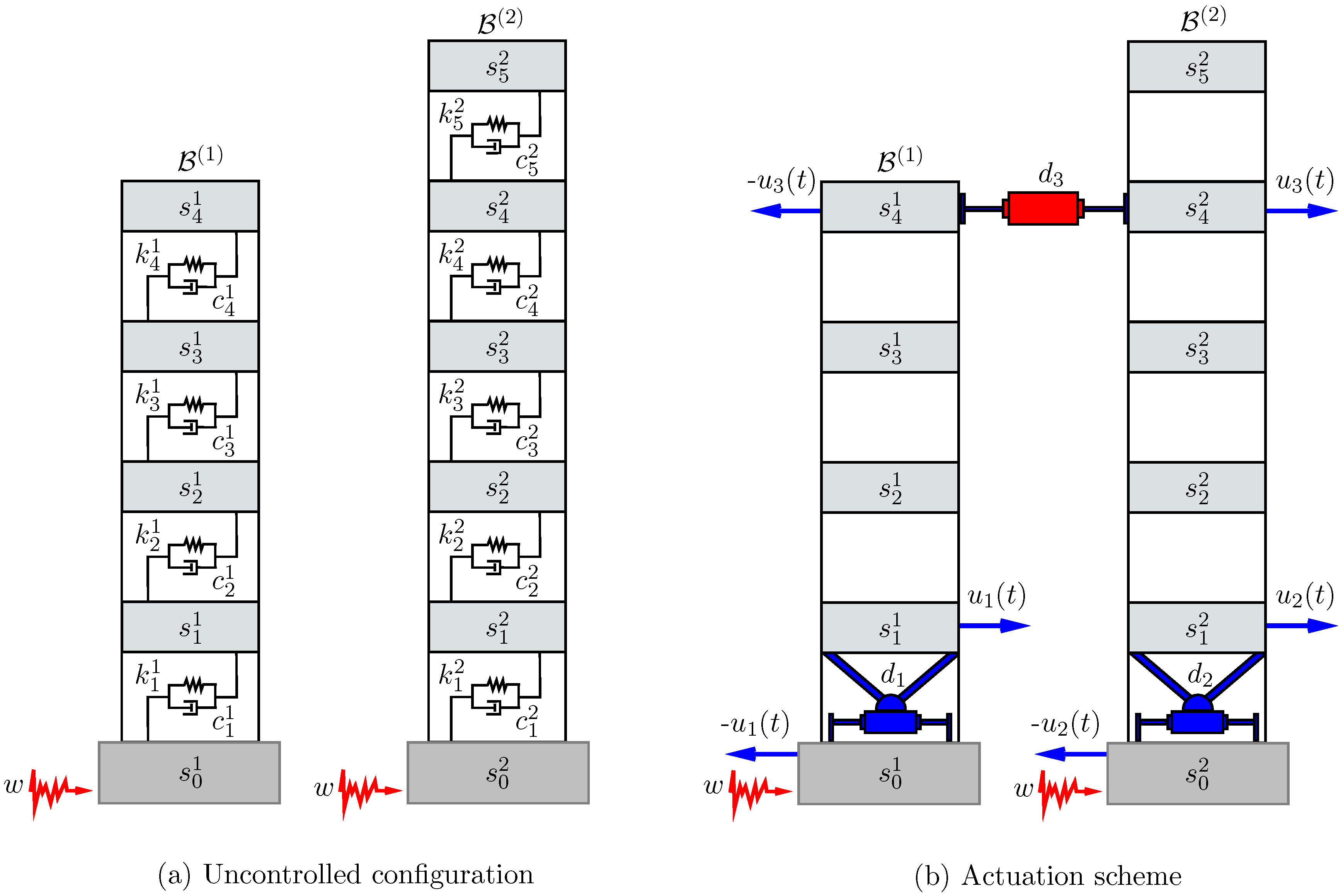
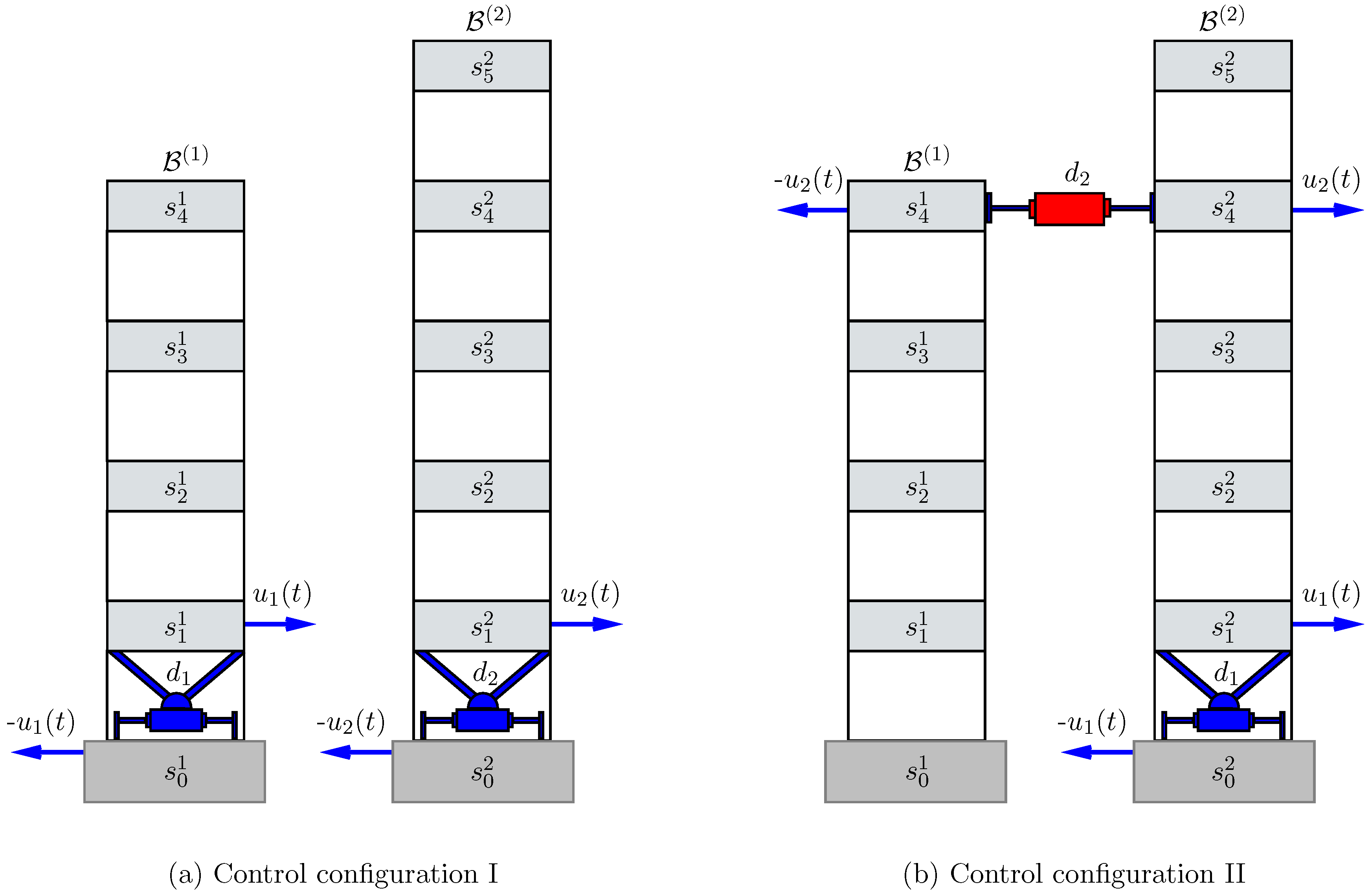
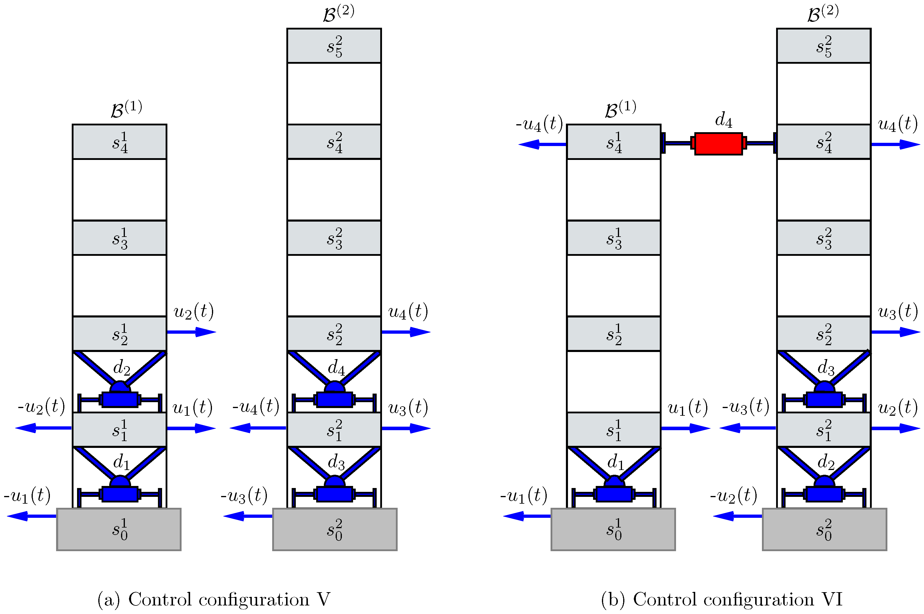
is the corresponding control location matrix. Thus, for the configuration CC6 displayed in Figure 4b, the number of actuation devices is n d = 4 and the measured-output vector has the form y ( t ) = [ y 1 ( t ) , y 2 ( t ) , y 3 ( t ) , y 4 ( t ) ] T , where y 1 ( t ) is the interstory velocity at the first-story level in building B ( 1 ) , y 2 ( t ) and y 3 ( t ) denote the interstory velocity at the first and second story levels in building B ( 2 ) , respectively, and y 4 ( t ) is the interbuilding velocity at the four-story level. In this case, by considering the matrix T u VI given in Equation (26), we obtain the measured-output matrix
C y VI = 0 0 0 0 0 0 0 0 0 1 0 0 0 0 0 0 0 0 0 0 0 0 0 0 0 0 0 0 0 0 0 1 0 0 0 0 0 0 0 0 0 0 0 0 0 0 0 0 0 1 1 0 0 0 0 0 0 0 0 0 0 0 0 0 0 0 1 0 0 0 1 0 .
To define the controlled-output vector z ( t ) , it should be noted that large interstory drifts and interbuilding approaches must both be avoided in order to prevent buildings’ structural damage and interbuilding collisions. Additionally, moderate control efforts are also convenient. To this end, we consider the controlled-output matrices
C z = α r C r α a C a [ 0 ] n d × 18 , D z = [ 0 ] 13 × n d α u I n d ,
where α r , α a and α u are scaling coefficients that compensate the different magnitude of interstory drifts, interbuilding approaches and control forces, respectively, C r and C a are the matrices given in Equation (19), and n d is the total number of actuation devices of the considered control configuration. With this choice, the controlled-output vector satisfies
z ( t ) 2 2 = α r 2 r ( t ) 2 2 + α a 2 a ( t ) 2 2 + α u 2 u ( t ) 2 2 .
To obtain a velocity-feedback H controller for the control configuration , we consider the system matrices A , B and E corresponding to the control location matrix T u , the mass and stiffness values given in Table A1 (see Appendix A) and the damping matrices in Equations (A1) and (A2); the measured-output matrix C y in Equation (31); and the controlled-output matrices C z and D z in Equation (33) defined by the corresponding control dimension n d and the scaling coefficients
α r = 5 , α a = 1 , α u = 10 7.4 .
Next, by applying the computational procedure described in Appendix B, we obtain a velocity-feedback control gain matrix K and an upper bound γ ˜ of the corresponding H -norm γ , which can be computed by considering the closed-loop transfer function T K ( 2 π f j ) 
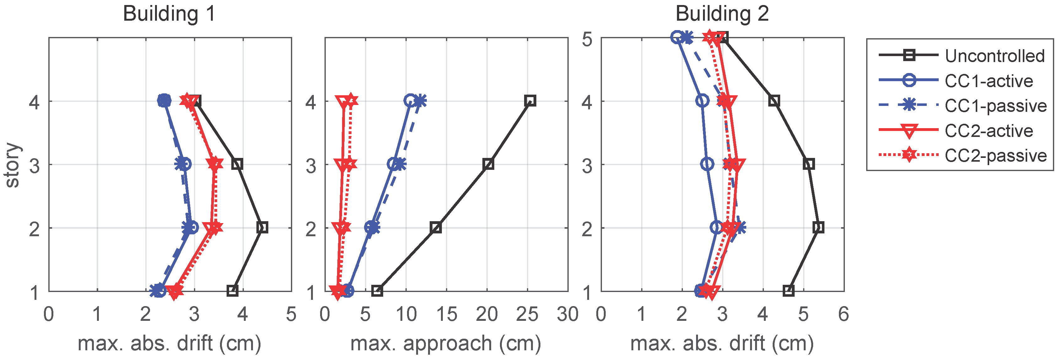
in Equation (A17) and solving the optimization problem given in Equation (A16). For the control configurations CC1 and CC2, we obtain the following velocity-feedback control gain matrices
K I = 10 7 × 0.7525 0.0142 0.8003 1.1890 , K II = 10 7 × 1.0176 0.0748 0.1392 0.4387 ,
and the γ -value upper bounds
γ ˜ I = 0.5973 , γ ˜ II = 0.8851 .
The actual γ -values are
γ I = 0.4967 , γ II = 0.7833 .
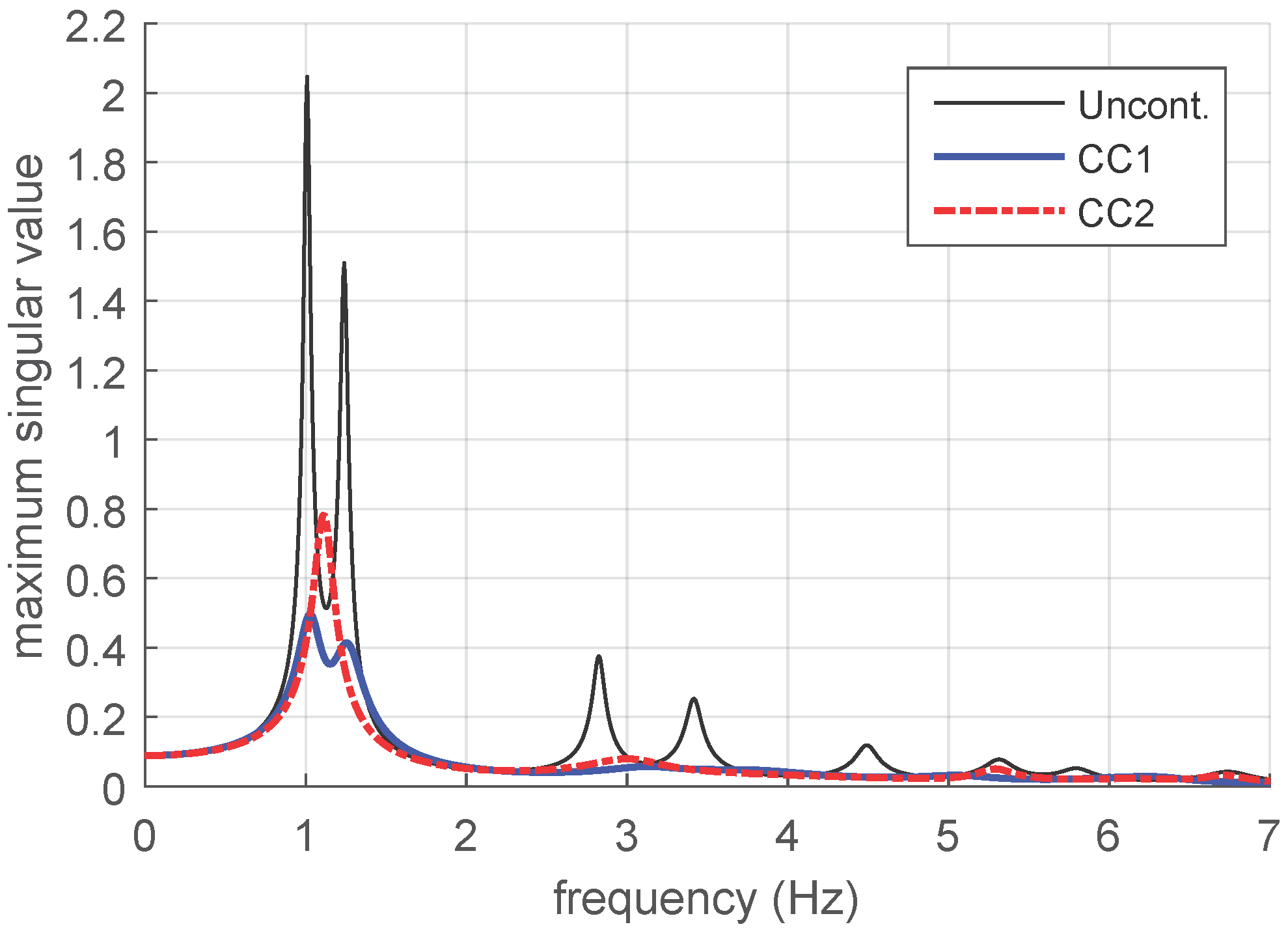
To illustrate the frequency behavior of the velocity-feedback controllers defined by the gain matrices K I and K II , the maximum singular values of the closed-loop transfer functions T K I ( 2 π f j ) , T K II ( 2 π f j ) and the open-loop transfer function
T ( 2 π f j ) = C z ( 2 π f j I A ) 1 E
are presented in Figure 5. In this figure, the thin black solid line displays the maximum singular values of the open-loop transfer function and shows the frequency response characteristics of the uncontrolled two-building structure. The peaks in this plot are associated to the natural resonant frequencies of the individual buildings, which are presented in Table 1. The main peak-value is associated to the frequency 1.0082 Hz and has a magnitude
γ 0 = 2.0479 ,
which corresponds to the H -norm of the uncontrolled configuration. The thick blue solid line presents the frequency response of the configuration CC1 with the velocity-feedback control gain matrix K I , and the red dash-dotted line shows the frequency response of the configuration CC2 with the velocity-feedback control gain matrix K II . As indicated in Equation (A16), the largest peak-values in these plots correspond to the controllers H -norms given in Equation (
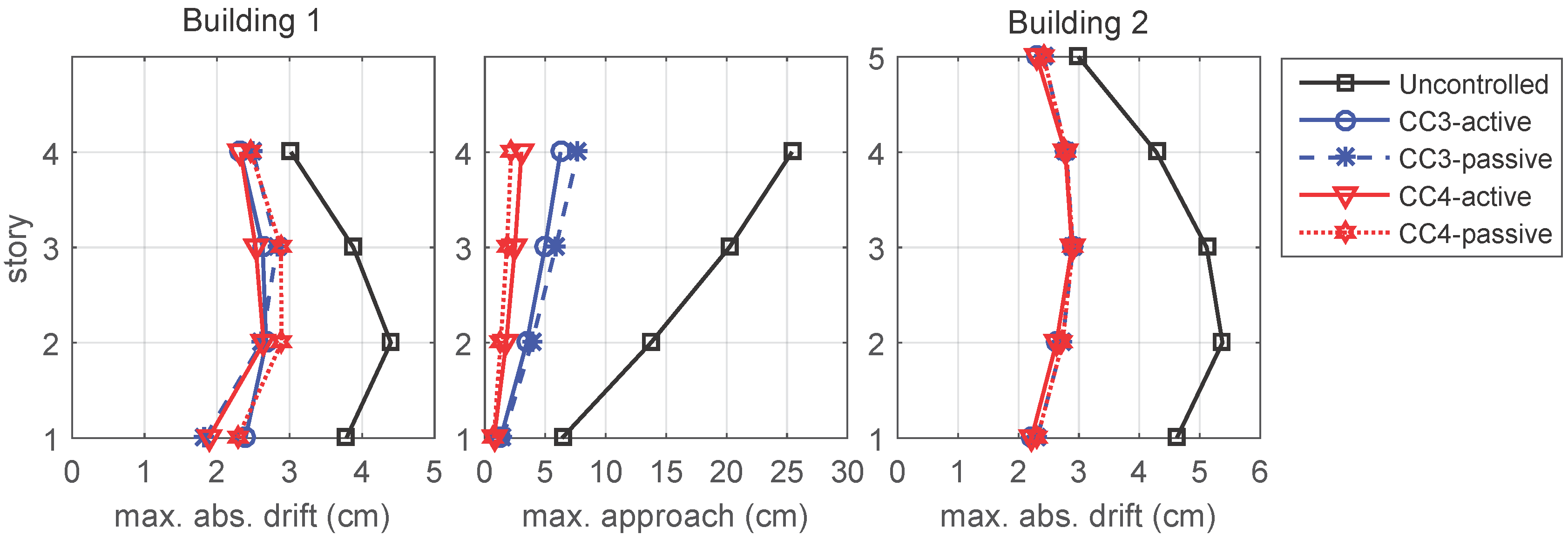
38). Following the same design procedure, we obtain the velocity-feedback control gain matrices
K III = 10 7 × 1.4671 0.3369 0.5595 0.0936 0.6758 0.4428 0.1090 0.5970 0.5382 , K IV = 10 6 × 6.8093 3.7631 0.3129 1.2553 8.6084 0.3653 0.5425 0.9675 2.9665 ,
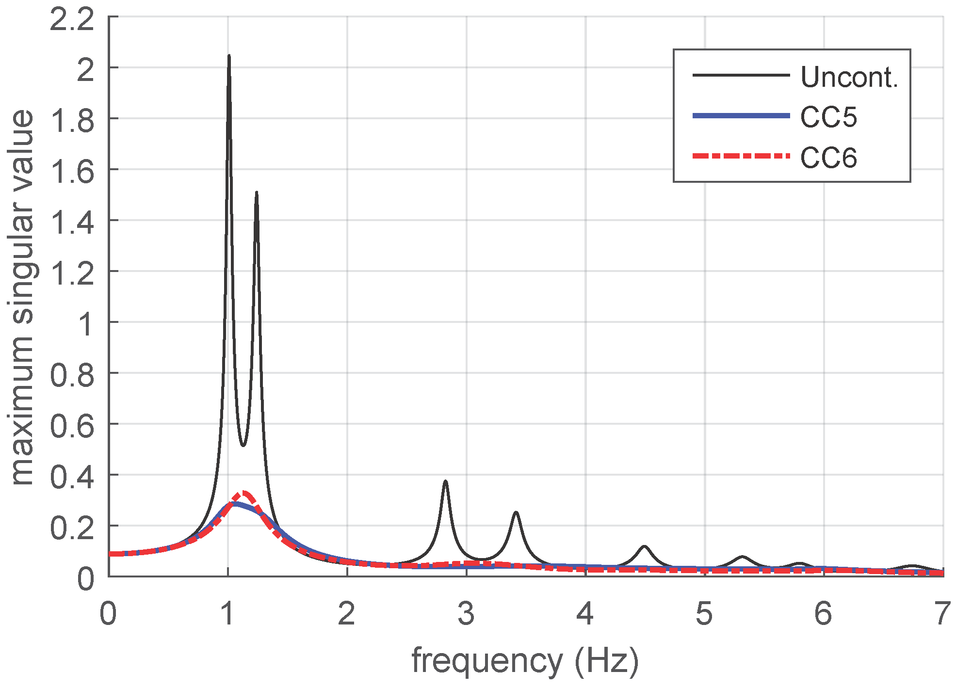
for the control configurations CC3 and CC4, respectively, the control gain matrix
K V = 10 7 × 1.0323 0.4066 0.2143 0.4538 0.3656 0.5823 0.3065 0.0591 0.9548 1.7601 1.5193 0.2758 0.3918 0.3666 0.5359 0.6302
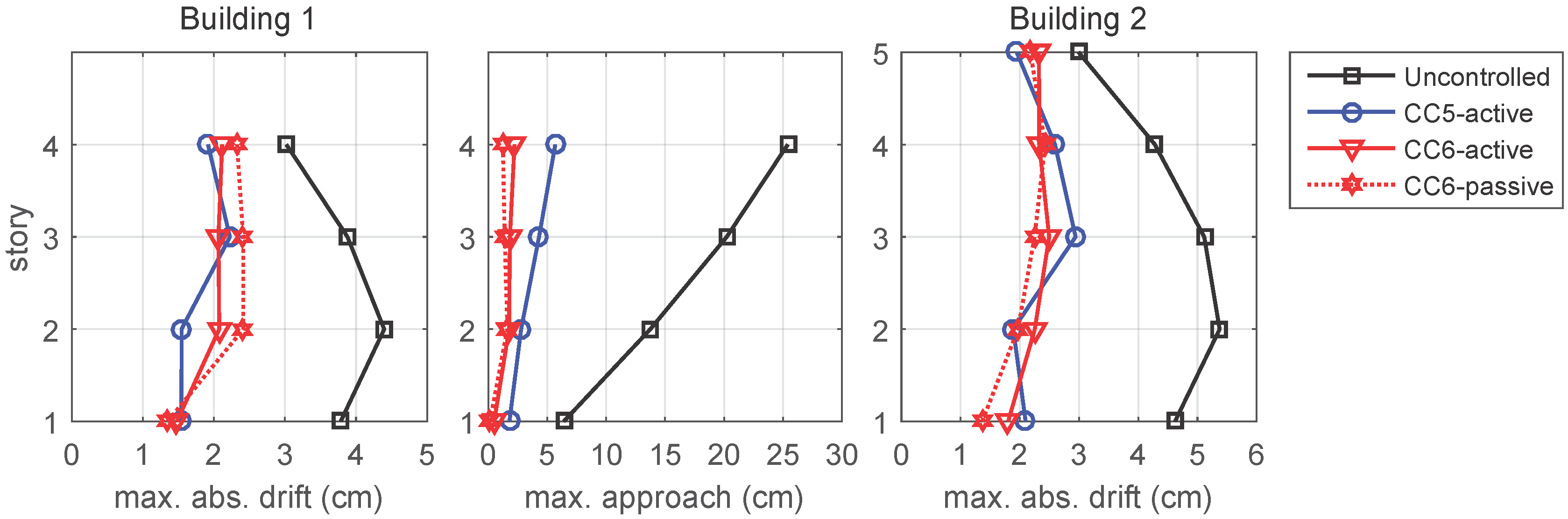
for the configuration CC5, and finally, the control gain matrix
K VI = 10 6 × 4.7133 4.9748 3.9433 1.9188 4.1747 5.9723 2.0281 1.4118 1.6926 4.8034 4.5185 0.1502 4.2366 3.2550 6.0731 6.8744
for the control configuration CC6. The corresponding γ -values and upper bounds γ ˜ are collected in 
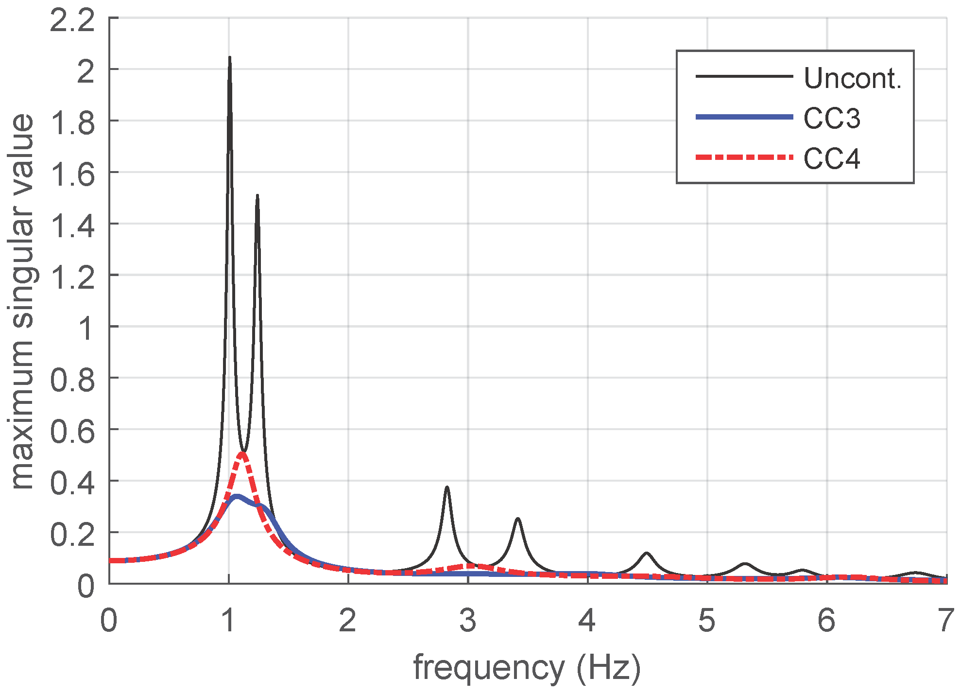
Table 2. The frequency responses are presented in Figure 6 and Figure 7, using a blue solid line for the unlinked configurations (CC3 and CC5), and a red dash-dotted line for the linked configurations (CC4 and CC6). According to the γ -values in Table 2 and the value γ 0 in Equation (40), three facts can be noted: (i) all the controllers obtained with the proposed design methodology provide a good level of reduction in the H -norm value, (ii) an increasing effectiveness is attained with a larger number of actuation devices, and (iii) smaller γ -values are obtained by the unlinked control configurations. All these facts can also be clearly appreciated by observing the peak-values in the frequency plots presented in Figure 5, Figure 6 and Figure 7. These frequency plots also show that, in all the cases, a significant reduction of the vibrational response is additionally attained in the secondary resonant peaks.

3.2. Static Velocity-Feedback H Decentralized Controllers

From a practical point of view, the controllers defined by the velocity-feedback gain matrices K computed in the previous section have the important advantage of using a reduced system of sensors which are naturally associated to the actuation devices. However, they also present two serious drawbacks. Firstly, the complete vector of measured outputs is used to compute the control actions and, consequently, a wide communication system would be necessary in the controller implementation. Secondly, producing the corresponding actuation forces would require active devices with a large power consumption and potential reliability issues. These two disadvantages, typically present in active vibration control of large structures, can be properly overcome by considering fully decentralized velocity-feedback controllers with control gain matrices of the form
K ^ = diag ( k ^ 1 , , k ^ n d ) ,
which can be obtained by solving the LMI optimization problem P in Equation (A8) with the same matrices used in the previous controller designs and constraining the LMI variable matrices X R and Y R to a diagonal form. As indicated in [17,40], if the gain matrix elements k ^ i 
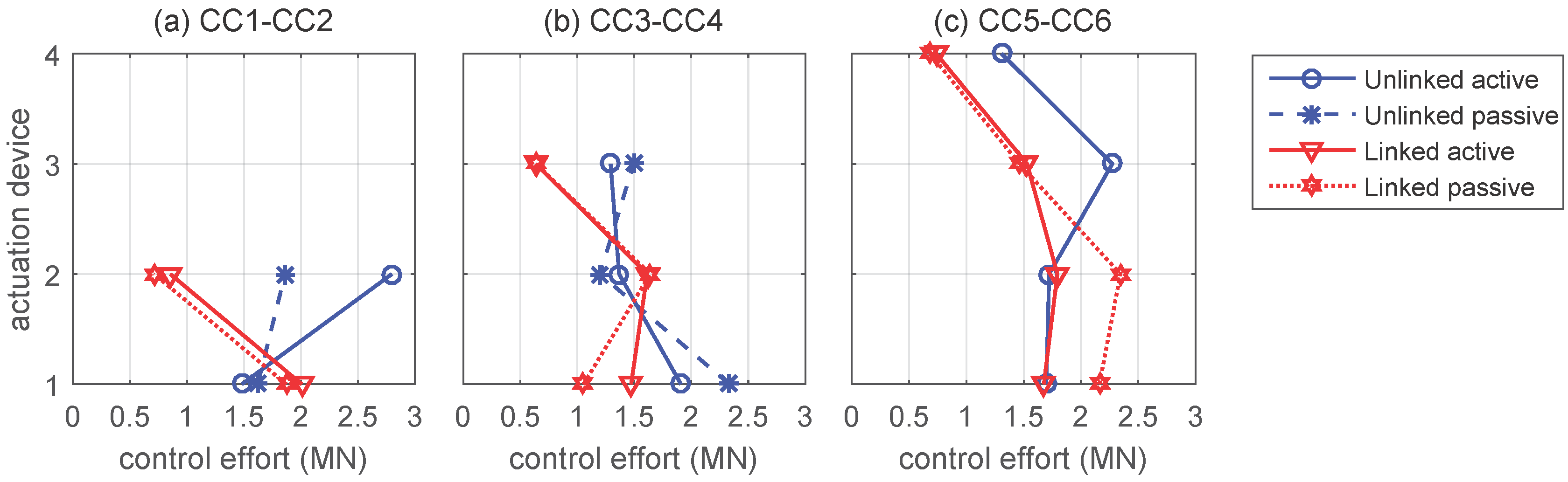
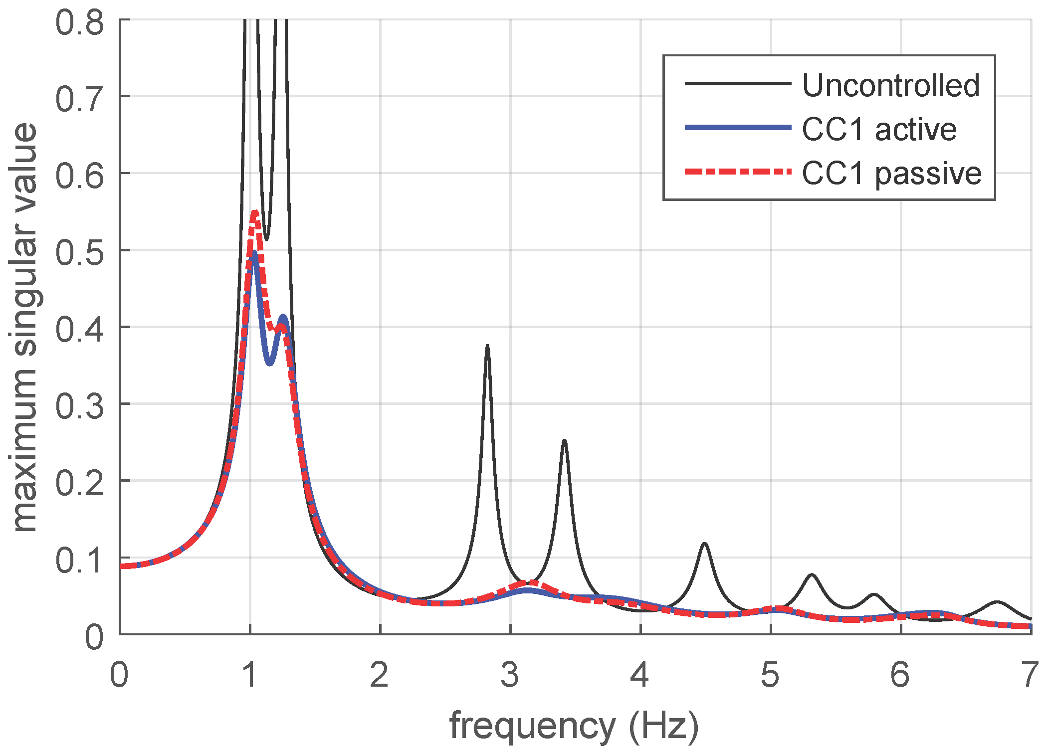
are all negative, then this kind of controllers admit a passive implementation using linear viscous dampers. Thus, for instance, by applying this design methodology to the control configuration CC1, we obtain the following diagonal gain matrix:
K ^ I = 10 7 × 0.8543 0 0 1.2968 .
Hence, the decentralized velocity-feedback controller defined by the diagonal gain matrix K ^ I can be implemented using two interstory linear damping devices d 1 and d 2 with respective damping constants 0.8543 × 10 7 Ns/m and 1.2968 × 10 7 Ns/m. The frequency response characteristics of this passive control system are displayed in Figure 8 using a red dash-dotted line. The frequency response corresponding to the uncontrolled configuration (thin black solid line) and the centralized controller defined by the gain matrix K I (thick blue solid line) are also included as a reference. The plots in the figure clearly show the good behavior of the obtained passive controller, which practically matches the performance of the active centralized controller over most of the frequency range, and produces a small increment (of about 10%) in the peak-value corresponding to the main resonant frequency.
Using the same design strategy to compute decentralized velocity-feedback controllers for the other control configurations considered in this paper, we have obtained diagonal gain matrices with the values presented in Table 3. Comparing the corresponding γ -values collected in Table 4 and the value γ 0 in Equation (40), it can be appreciated that the same three facts observed in the centralized controller designs also apply to the decentralized controllers: (i) all the controllers obtained with the proposed design methodology provide a good level of reduction in the H -norm value, (ii) an increasing effectiveness is attained with a larger number of actuation devices, and (iii) smaller γ -values are obtained by the unlinked control configurations. However, two new elements appear in the decentralized design: (iv) the risk of failure of the controller design procedure is higher in the decentralized designs, and (v) the γ -value attained by some decentralized controllers is lower than the one obtained by the associated centralized controller.
The increased risk of failure in the decentralized design procedure can be explained by the additional structure constraints introduced in the LMI optimization problem, which can produce feasibility issues. This kind of numerical problems are poorly understood and sometimes depend on the particular numerical solver and the options used in the LMI optimization procedure. In our case, the feasibility issues have only been encountered in the design of a diagonal gain matrix for the control configuration CC5. Regarding the γ -value produced by some decentralized controllers, by comparing the γ -values in Table 2 and Table 4, it can be seen that a lower γ -
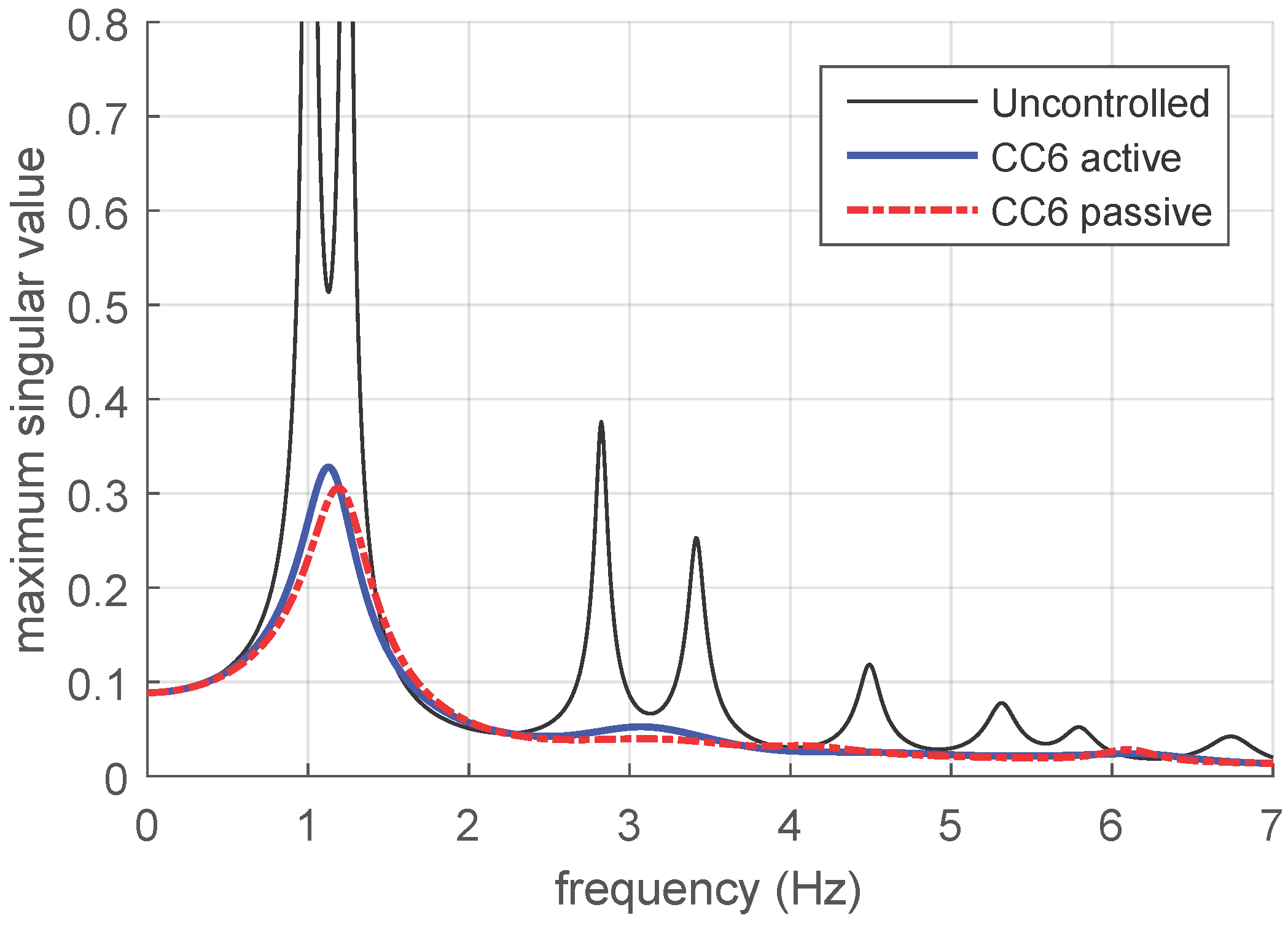
value is attained by the decentralized controllers for the control configurations CC2, CC3 and CC6. A clear view of this situation can be obtained in Figure 9, which presents the frequency response corresponding to the passive control system defined by the diagonal gain matrix K ^ VI (red dash-dotted line) and the corresponding centralized controller defined by the gain matrix K VI given in Equation (43) (thick blue solid line). To explain this unexpected fact, it should be noted that the LMI optimization procedure is based on the upper bound γ ˜ and produces a suboptimal H controller. Obviously, the upper bound γ ˜ ( K ) corresponding to the unstructured gain matrix K must be inferior to the upper bound γ ˜ ( K ^ ) obtained for the diagonal gain matrix K ^ , which has been computed by solving a constrained version of the same LMI optimization problem. Looking at the data in Table 2 and Table 4, we can see that the inequality γ ˜ ( K ) γ ˜ ( K ^ ) certainly holds for all the control configurations. Additionally, the actual γ -values γ ( K ) and γ ( K ^ ) must satisfy γ ( K ) γ ˜ ( K ) and γ ( K ^ ) γ ˜ ( K ^ ) . However, these inequalities do not exclude the observed fact that γ ( K ^ ) < γ ( K ) . That is, they do not exclude the unexpected possibility of obtaining a passive controller with a better performance than the corresponding active controller.
Remark 1.
In this paper, all the computations have been carried out using Matlab © R2015b on a regular laptop with an Intel © Core T M i7-2640M processor at 2.80 GHz. The LMI optimization problems corresponding to the different controller designs have been solved with the function mincx() included in the Robust Control Toolbox T M . A relative accuracy of 10 7 has been set in the solver options.

4. Numerical Simulations

In this section, a proper set of numerical simulations is conducted to investigate the vibrational time-response of the two-building system for the considered control configurations. The simulations include the active controllers designed in Section 3.1, the passive controllers computed in Section 3.2 and the response of the uncontrolled buildings, which is taken as a natural reference in the performance assessment. In all the cases, the full-scale North–South El Centro 1940 ground acceleration seismic record (see Figure 10) has been used as external disturbance. To describe the vibrational response of the individual buildings and the buildings interactions, the vectors of interstory drifts r ( t ) and interbuilding approaches a ( t ) have been computed. Additionally, the vector of control efforts u ( t ) has also been computed for the controlled configurations. Overall, the simulations include eleven different control configurations plus the uncontrolled case. To provide an intuitive and effective summary of this complex set of numerical results, the control configurations have been grouped by the number of actuation devices. Thus, the peak-values of the absolute interstory drifts and interbuilding approaches corresponding to the control configurations with two actuation devices (CC1 and CC2) are presented in Figure 11, where the interstory drift peak-values corresponding to the four-story building B ( 1 ) are presented in the left-hand-side graphic, the interbuilding approach peak-values are shown in the central graphic, and the interstory drift peak-values corresponding to the five-story building B ( 2 ) are displayed in the right-hand-side graphic. In the graphics of this section, the following colors and line styles have been used: blue lines present the values of the unlinked control configurations, red lines represent the linked control configurations, and black lines correspond to the uncontrolled configuration; additionally, active controllers are represented by solid lines, and passive controllers by non-solid lines. Detailed legends and captions have also been included in the figures to facilitate an unambiguous interpretation of the graphics. Specifically, the following colors, line styles and symbols have been used in the plots of Figure 11: black solid line with squares for the uncontrolled configuration, blue solid line with circles for the unlinked control configuration CC1 with the active controller defined by the control gain matrix K I given in Equation (36), blue dashed line with asterisks for the unlinked control configuration CC1 with the passive controller defined by the control gain matrix K ^ I given in Equation (45), red solid line with triangles for the linked control configuration CC2 with the active controller defined by the control gain matrix K II given in Equation (36), and red dotted line with hexagrams for the linked control configuration CC2 with the passive controller defined by the control gain matrix K ^ II given in Table 3. The peak-values of the corresponding absolute control efforts are presented in Figure 12a. Looking at graphics in Figure 11 and Figure 12a, the following facts can be clearly appreciated: (i) all the controllers provide a significant level of reduction in the interstory drift and interbuilding approach peak-values when compared with the uncontrolled response; (ii) the unlinked control configuration CC1 is more effective in mitigating the interstory drift response; (iii) the linked control configuration CC2 attains better results in reducing the interbuilding approaches; (iv) smaller control-effort peak-values are produced by the linked configuration CC2; and (v) the levels of performance attained by the passive controllers are quite similar to those achieved by the corresponding active controllers, especially in the case of the linked control configuration CC2.
For the control configurations with three actuation devices CC3 and CC4, the plots of interstory drift and interbuilding approach peak-values presented in Figure 13 show that the best overall behavior corresponds to the linked control configuration CC4 with the active controller defined by the control gain matrix K IV given in Equation (41) (red solid line with triangles). Also remarkable is the overall performance of the linked control configuration CC4 with the passive controller defined by the control gain matrix K ^ IV given in Table 3 (red dotted line with hexagrams). Moreover, looking at the plots shown in Figure 12b, it can be appreciated that smaller control-effort peak-values are required by the controllers corresponding to the linked control configuration CC4. For the control configurations with four actuation devices CC5 and CC6, the plots of interstory drift and interbuilding approach peak-values presented in Figure 14 and the control-effort peak-values displayed in Figure 12c indicate the superior performance of the linked control configuration CC6 with the active controller defined by the control gain matrix K VI given in Equation (43). The good properties of this linked control configuration with the passive controller K ^ VI can also be clearly appreciated. It should be recalled that feasibility issues appeared in the design of a fully decentralized velocity-feedback controller for the unlinked control configuration CC5 and, consequently, no passive controller is available for this case.
To complement the information supplied by the interstory drift and the interbuilding approach time responses, the absolute acceleration peak-values of the buildings’ top-level stories corresponding to the proposed active and passive velocity-feedback controllers are presented in Table 5 and Table 6, respectively. Additionally, to provide a wider vision of the acceleration response characteristics, the story absolute acceleration peak-values corresponding to the uncontrolled configuration and the active and passive controllers proposed for the control configurations CC3 and CC4 are displayed in Figure 15. Looking at the values of building B ( 1 ) in Table 5, it can be appreciated that better results are attained by the linked control configurations. In this case, the best performance is achieved by the linked configuration CC6, which produces a 50.6% of reduction with respect to the uncontrolled response. In contrast, the values of building B ( 2 ) indicate a better behavior of the unlinked control configurations. For this building, the best performance corresponds to the unlinked control configuration CC3, which produces a 45.5% of reduction with respect to the uncontrolled response. Looking at the data in Table 6, a similar pattern can be appreciated in the values produced by the passive controllers. In this case, the best results are attained by the linked configuration CC4 in building B ( 1 ) , which produces a 39.7% of reduction with respect to the uncontrolled response, and by the unlinked configuration CC3 in building B ( 2 ) , with a relative reduction of 43.1%. These acceleration response characteristics are further illustrated by the plots in Figure 15, where the following facts can be clearly appreciated: (i) all the proposed controllers produce positive results in reducing the story absolute acceleration peak-values when compared with the uncontrolled response; (ii) the unlinked control configuration CC3 is more effective in mitigating the acceleration response of the taller building B ( 2 ) ; (iii) the linked control configuration CC4 attains better results in reducing the acceleration response of the shorter building B ( 1 ) ; and (iv) the levels of performance of the passive controllers are similar to those attained by the corresponding active controllers, especially in the case of the linked control configuration CC4.
Remark 2.
In order to avoid the modeling and simulation difficulties associated to interbuilding collisions, the numerical simulations have been carried out assuming that the interbuilding spacing is large enough to prevent pounding events. In this case, the maximum interbuilding approaches can be understood as lower bounds of safe interbuilding distances. Thus, for example, the central plots in Figure 14 point out that, for the considered seismic event, an interbuilding distance of 2.5 cm can be considered safe for the active and passive controllers of the linked control configuration CC6 while, in contrast, an interbuilding separation of 5 cm would produce interbuilding collisions for the active controller of the unlinked control configuration CC5. For the uncontrolled configuration, a interbuilding gap of more than 25 cm would have been necessary to avoid pounding events.
Remark 3.
It should be noted that the linked control configuration CC2 is an incomplete actuation scheme, in the sense that it does not include any interstory actuation device in building B ( 1 ) . This element can possibly help to explain its reduced effectiveness in mitigating the interstory drift response. In contrast, all the other control configurations include a more balanced actuation scheme with interstory actuation devices in both buildings.
Remark 4.
Although no general conclusions can be drawn from the considered particular configurations, the obtained numerical results seem to indicate that the presence of interbuilding actuation devices can produce opposite effects in the acceleration response of linked buildings with a different height. This fact certainly opens a number of interesting questions related to the acceleration response characteristics of linked buildings, such as the relevance of the height difference, the behavior of linked buildings with the same height, and the effect of multiple linking devices.

5. Conclusions and Future Directions

In this paper, the design of advanced structural vibration control systems for the seismic protection of adjacent multi-story buildings has been investigated. The proposed approach considers multi-actuation schemes that combine interstory and interbuilding force actuation devices implemented at different locations of the structure. Using an advanced static output-feedback H controller design methodology, active and passive vibration control systems have been obtained for a multi-story two-building structure equipped with a selected set of linked and unlinked actuation schemes. After studying the corresponding frequency and time responses, the following positive points can be highlighted: (i) The proposed design methodology allows dealing with a wide variety of actuation schemes. (ii) The obtained control systems provide a significant reduction of the frequency response in the main and secondary resonant modes. Moreover, they also produce a significant reduction of the maximum interbuilding approaches and the absolute interstory drift peak-values in both buildings. (iii) The obtained control systems produce positive results in reducing the buildings acceleration responses. (iv) Control configurations with interbuilding linking devices provide a higher protection against pounding events and produce lower control-effort peak-values. (v) Lower interstory drift peak-values are attained in buildings equipped with interstory actuation devices. (vi) A remarkable performance level is achieved by the passive control systems. (vii) In general, more effective and better balanced results are obtained with a larger number of actuation devices. Additionally, the following negative aspects can be pointed out: (viii) The design procedure can fail due to feasibility issues in the associated LMI optimization problem, specially in the constrained passive designs. (ix) The controller H -norm is a suitable index to obtain effective controllers, but it cannot be used to identify optimal configurations of the actuation system. (x) Due to the computational cost and complexity, the proposed design methodology is only effective for structures with a moderate number of stories.
In summary, the observed results indicate the convenience of using multi-actuation systems that combine interbuilding linking devices and interstory actuators implemented in both buildings. The good behavior exhibited by the obtained passive control systems is a fact of singular relevance, which certainly deserves a deeper investigation. Further research effort should also be invested in studying the acceleration response of linked buildings, and in performing more realistic numerical simulations, which should include the effect of pounding events and other nonlinear aspects. Finally, it is worth mentioning the important open problem of finding a suitable methodology to determine the optimal configuration of distributed multi-actuation systems in large-scale structures.

Acknowledgments

This work was partially supported by the Spanish Ministry of Economy and Competitiveness under Grant DPI2015-64170-R/FEDER.

Author Contributions

All the authors contributed to the modeling and the scientific elaboration. Moreover, J. M. Rossell and J. Rubió-Massegú designed the centralized controllers; H. R. Karimi designed the decentralized controllers and computed the frequency responses; F. Palacios-Quiñonero and J. Rubió-Massegú performed the numerical simulations; F. Palacios-Quiñonero, in collaboration with the other authors, wrote the paper.

Conflicts of Interest

The authors declare no conflict of interest.

Appendix A. Buildings Parameters

Table A1. Mass and stiffness coefficient values corresponding to the two-building system.
Building B ( 1 ) Building B ( 2 )
Story123412345
mass ( × 10 5 Kg)2.1522.0922.0702.6612.1522.0922.0702.0482.661
stiffness ( × 10 8 N/m)1.4701.1300.9900.8401.4701.1300.9900.8900.840
In this appendix, the particular parameter values of the two-building system used in the controller designs and numerical simulations are presented. The mass and stiffness coefficients are collected in Table A1. These values are similar to those presented in [42]. Approximate damping matrices C d ( 1 ) and C d ( 2 ) have been computed following a Rayleigh damping approach [41], by setting a 2% of relative damping on the corresponding smallest and largest modes. The obtained particular values (in Ns/m) are the following:
C d ( 1 ) = 10 5 × 2.6450 0.9034 0 0 0.9034 2.2455 0.7915 0 0 0.7915 2.0078 0.6715 0 0 0.6715 1.3719 ,
C d ( 2 ) = 10 5 × 2.6017 0.9244 0 0 0 0.9244 2.1958 0.8099 0 0 0 0.8099 1.9946 0.7281 0 0 0 0.7281 1.8670 0.6872 0 0 0 0.6872 1.2741 .

Appendix B. Static Output-Feedback H Controller Design

This appendix provides a brief summary of the static output-feedback H controller design methodology presented in [38,39]. Let us consider the linear model
x ˙ ( t ) = A x ( t ) + B u ( t ) + E w ( t ) z ( t ) = C z x ( t ) + D z u ( t ) y ( t ) = C y x ( t )
where x ( t ) is the state, u ( t ) is the control action, w ( t ) is the external disturbance, z ( t ) is the controlled output, and y ( t ) is the measured output. The design objective is to obtain an optimal static output-feedback H controller
u ( t ) = K y ( t )
that produces an asymptotically stable closed-loop matrix
A K = A + B K C y
and, simultaneously, minimizes the associated H -norm
γ K = sup w 2 0 z 2 w 2 ,
where f 2 = 0 f T ( t ) f ( t ) d t 1 / 2 denotes the usual continuous 2-norm. Computing this kind of optimal controllers is a challenging problem that still remains open. However, according to the results in [38,39], a suboptimal static output-feedback H controller
u ( t ) = K ˜ y ( t )
can be computed by solving the following LMI optimization problem:
P : { maximize   η subject to  X Q > 0 ,   X R > 0 ,   η > 0  and the LMI in  A9 ,
A Q X Q Q T + Q X Q Q T A T + A R X R R T + R X R R T A T + B Y R R T + R Y R T B T + η E E T * C z Q X Q Q T + C z R X R R T + D z Y R R T I < 0 ,
where * denotes the transpose of the symmetric entry, X Q , X R and Y R are the optimization variables, Q is a matrix whose columns contain a basis of Ker ( C y ) , and the matrix R has the following form:
R = C y + Q L ˜ , L ˜ = Q X ˜ C y T C y X ˜ C y T 1 ,
where
C y = C y T C y C y T 1 , Q = Q T Q 1 Q T
are the Moore-Penrose pseudoinverses of C y and Q , respectively, and X ˜ is the optimal X-matrix of the auxiliary LMI optimization problem
P a : { maximize  η a subject to  X > 0 ,   η a > 0  and the LMI in  A13 ,
A X + X A T + B Y + Y T B T + η a E E T * C z X + D z Y I < 0 .
If an optimal value η ˜ is attained in P for the triplet ( X ˜ Q , X ˜ R , Y ˜ R ) , then the output gain matrix K ˜ can be written in the form
K ˜ = Y ˜ R X ˜ R 1 .
Moreover, the value
γ ˜ K ˜ = η ˜ 1 / 2
provides an upper bound of the associated H -norm γ K ˜ , which can be computed by solving the optimization problem
γ K ˜ = sup f σ max T K ˜ ( 2 π f j ) ,
where j = 1 , f is the frequency in hertz, σ max [ · ] denotes the maximum singular value and
T K ˜ ( s ) = C K ˜ ( s I A K ˜ ) 1 E ,
with
A K ˜ = A + B K ˜ C y , C K ˜ = C z + D z K ˜ C y ,
is the closed-loop transfer function from the disturbance input to the controlled output.

References

  1. Abdel Raheem, S.E. Mitigation measures for earthquake induced pounding effects on seismic performance of adjacent buildings. Bull. Earthq. Eng. 2014, 12, 1705–1724. [Google Scholar] [CrossRef]
  2. Kandemir-Mazanoglu, E.C.; Mazanoglu, K. An optimization study for viscous dampers between adjacent buildings. Mech. Syst. Signal Process. 2017, 89, 88–96. [Google Scholar] [CrossRef]
  3. Kumar, P.; Karuna, S. Effect of seismic pounding between adjacent buildings and mitigation measures. Int. J. Res. Eng. Technol. 2015, 4, 208–216. [Google Scholar]
  4. Pawar, P.D.; Murnal, P.B. Effect of seismic pounding on adjacent buildings considering soil-structure interaction. Int. J. Adv. Found. Res. Sci. Eng. 2015, 2, 286–294. [Google Scholar]
  5. Sorace, S.; Terenzi, G. Damped interconnection-based mitigation of seismic pounding between adjacent R/C buildings. LACSIT Int. J. Eng. Technol. 2013, 5, 406–412. [Google Scholar] [CrossRef]
  6. Tubaldi, E.; Freddi, F.; Barbato, M. Probabilistic seismic demand model for pounding risk assessment. Earthq. Eng. Struct. Dyn. 2016, 45, 1743–1758. [Google Scholar] [CrossRef]
  7. McCall, A.J.; Balling, R.J. Structural analysis and optimization of tall buildings connected with skybridges and atria. Struct. Multidiscip. Optim. 2016, 55, 583–600. [Google Scholar] [CrossRef]
  8. Pardalopoulos, S.I.; Pantazopoulou, S.J. Seismic response of nonstructural components attached on multistorey buildings. Earthq. Eng. Struct. Dyn. 2015, 44, 139–158. [Google Scholar] [CrossRef]
  9. Behnamfar, F.; Dorafshan, S.; Taheri, A.; Hashemi, B.H. A method for rapid estimation of dynamic coupling and spectral responses of connected adjacent structures. Struct. Des. Tall Spec. Build. 2016, 25, 605–625. [Google Scholar] [CrossRef]
  10. Tubaldi, E. Dynamic behavior of adjacent buildings connected by linear viscous/viscoelastic dampers. Struct. Control Health Monit. 2015, 22, 1086–1102. [Google Scholar] [CrossRef]
  11. Patel, C.C.; Jangid, R.S. Dynamic response of identical adjacent structures connected by viscous damper. Struct. Control Health Monit. 2014, 21, 205–224. [Google Scholar] [CrossRef]
  12. Richardson, A.; Walsh, K.K.; Abdullah, M.M. Closed-form equations for coupling linear structures using stiffness and damping elements. Struct. Control Health Monit. 2013, 20, 259–281. [Google Scholar] [CrossRef]
  13. Jankowski, R.; Mahmoud, S. Linking of adjacent three-storey buildings for mitigation of structural pounding during earthquakes. Bull. Earthq. Eng. 2016, 14, 3075–3097. [Google Scholar] [CrossRef]
  14. Bigdeli, K.; Hare, W.; Nutini, J.; Tesfamariam, S. Optimizing damper connectors for adjacent buildings. Optim. Eng. 2016, 17, 47–75. [Google Scholar] [CrossRef]
  15. Greco, R.; Marano, G.C. Multi-objective optimization of a dissipative connection for seismic protection of wall-frame structures. Soil Dyn. Earthq. Eng. 2016, 87, 151–163. [Google Scholar] [CrossRef]
  16. Yang, Z.D.; Lam, E.S.S. Dynamic responses of two buildings connected by viscoelastic dampers under bidirectional earthquake excitations. Earthq. Eng. Eng. Vib. 2014, 13, 137–150. [Google Scholar] [CrossRef]
  17. Palacios-Quiñonero, F.; Rubió-Massegú, J.; Rossell, J.M.; Karimi, H.R. Vibration control for adjacent structures using local state information. Mechatronics 2014, 24, 336–344. [Google Scholar] [CrossRef]
  18. Huang, X.; Zhu, H. Optimal arrangement of viscoelastic dampers for seismic control of adjacent shear-type structures. J. Zhejiang Univ. Sci. A 2013, 14, 47–60. [Google Scholar] [CrossRef]
  19. Tehrani, M.G.; Gattulli, V. Vibration control using nonlinear damped coupling. J. Phys. Conf. Ser. 2016, 744, 1–9. [Google Scholar] [CrossRef]
  20. Kasagi, M.; Fujita, K.; Tsuji, M.; Takewaki, I. Effect of non-linearity of connecting dampers on vibration control of connected building structures. Front. Built Environ. 2016, 1, 1–9. [Google Scholar] [CrossRef]
  21. Uz, M.E.; Sharafi, P. Investigation of the optimal semi-active control strategies of adjacent buildings connected with magnetorheological dampers. Int. J. Optim. Civ. Eng. 2016, 6, 523–547. [Google Scholar]
  22. Abdeddaim, M.; Ounis, A.; Djedoui, N.; Shrimali, M.K. Pounding hazard mitigation between adjacent planar buildings using coupling strategy. J. Civ. Struct. Health Monit. 2016, 6, 603–617. [Google Scholar] [CrossRef]
  23. Uz, M.E.; Hadi, M.N.S. Optimal design of semi active control for adjacent buildings connected by MR damper based on integrated fuzzy logic and multi-objective genetic algorithm. Eng. Struct. 2014, 69, 135–148. [Google Scholar] [CrossRef]
  24. Kim, H.S. Seismic response control of adjacent buildings coupled by semi-active shared TMD. Int. J. Steel Struct. 2016, 16, 647–656. [Google Scholar] [CrossRef]
  25. Sun, H.; Liu, M.; Zhu, H. Connecting parameters optimization on unsymmetrical twin-tower structure linked by sky-bridge. J. Cent. South Univ. 2014, 21, 2460–2468. [Google Scholar] [CrossRef]
  26. Kim, H.S.; Kim, Y.J. Control performance evaluation of shared tuned mass damper. Adv. Sci. Technol. Lett. 2014, 69, 1–4. [Google Scholar]
  27. Gao, H.; Zhan, W.; Karimi, H.R.; Yang, X.; Yin, S. Allocation of actuators and sensors for coupled- adjacent-building vibration attenuation. IEEE Trans. Ind. Electron. 2013, 60, 5792–5801. [Google Scholar] [CrossRef]
  28. Park, K.S.; Ok, S.Y. Optimal design of actively controlled adjacent structures for balancing the mutually conflicting objectives in design preference aspects. Eng. Struct. 2012, 45, 213–222. [Google Scholar] [CrossRef]
  29. Dumne, S.M.; Shrimali, M.K.; Bharti, S.D. Earthquake performance of hybrid controls for coupled buildings with MR dampers and sliding base isolation. Asian J. Civ. Eng. 2017, 18, 63–97. [Google Scholar]
  30. Fathi, F.; Bahar, O. Hybrid coupled building control for similar adjacent buildings. KSCE J. Civ. Eng. 2017, 21, 265–273. [Google Scholar] [CrossRef]
  31. Kasagi, M.; Fujita, K.; Tsuji, M.; Takewaki, I. Automatic generation of smart earthquake-resistant building system: Hybrid system of base-isolation and building-connection. Helyon 2016, 2, 1–21. [Google Scholar] [CrossRef] [PubMed]
  32. Shrimali, M.K.; Bharti, S.D.; Dumne, S.M. Seismic response analysis of coupled building involving MR damper and elastomeric base isolation. Ain Shams Eng. J. 2015, 6, 457–470. [Google Scholar] [CrossRef]
  33. Murase, M.; Tsuji, M.; Takewaki, I. Smart passive control of buildings with higher redundancy and robustness using base-isolation and inter-connection. Earthq. Struct. 2013, 4, 649–670. [Google Scholar] [CrossRef]
  34. Taniguchi, M.; Fujita, K.; Tsuji, M.; Takewaki, I. Hybrid control system for greater resilience using multiple isolation and building connection. Front. Built Environ. 2016, 2, 1–10. [Google Scholar] [CrossRef]
  35. Tubaldi, E.; Barbato, M.; Dall’Asta, A. Efficient approach for the reliability-based design of linear damping devices for seismic protection of buildings. ASCE-ASME J. Risk Uncertain. Eng. Syst. Part A Civ. Eng. 2016, 2, 1–10. [Google Scholar] [CrossRef]
  36. Park, K.S.; Ok, S.Y. Optimal design of hybrid control system for new and old neighboring buildings. J. Sound Vib. 2015, 336, 16–31. [Google Scholar] [CrossRef]
  37. Park, K.S.; Ok, S.Y. Hybrid control approach for seismic coupling of two similar adjacent structures. J. Sound Vib. 2015, 349, 1–17. [Google Scholar] [CrossRef]
  38. Rubió-Massegú, J.; Rossell, J.M.; Karimi, H.R.; Palacios-Quiñonero, F. Static output-feedback control under information structure constraints. Automatica 2013, 49, 313–316. [Google Scholar] [CrossRef]
  39. Palacios-Quiñonero, F.; Rubió-Massegú, J.; Rossell, J.M.; Karimi, H.R. Feasibility issues in static output-feedback controller design with application to structural vibration control. J. Frankl. Inst. 2014, 351, 139–155. [Google Scholar] [CrossRef]
  40. Palacios-Quiñonero, F.; Rubió-Massegú, J.; Rossell, J.M.; Karimi, H.R. Optimal passive-damping design using a decentralized velocity-feedback H approach. Model. Identif. Control 2012, 33, 87–97. [Google Scholar] [CrossRef]
  41. Chopra, A. Dynamics of Structures. Theory and Applications to Earthquake Engineering, 3rd ed.; Prentice Hall: Upper Saddle River, NJ, USA, 2007. [Google Scholar]
  42. Kurata, N.; Kobori, T.; Takahashi, M.; Niwa, N.; Midorikawa, H. Actual seismic response controlled building with semi-active damper system. Earthq. Eng. Struct. Dyn. 1999, 28, 1427–1447. [Google Scholar] [CrossRef]
Figure 1. Two-building model: (a) Uncontrolled configuration. (b) Linked actuation scheme formed by two interstory actuators ( d 1 and d 2 ) and one interbuilding actuator ( d 3 ).
Applsci 07 00323 g001
Figure 2. Actuation schemes with two actuation devices. (a) Unlinked configuration CC1, with two interstory actuators ( d 1 and d 2 ). (b) Linked configuration CC2, with an interstory actuator ( d 1 ) and an interbuilding actuator ( d 2 ).
Applsci 07 00323 g002
Figure 3. Actuation schemes with three actuation devices. (a) Unlinked configuration CC3, with three interstory actuators ( d 1 , d 2 and d 3 ). (b) Linked configuration CC4, with two interstory actuators ( d 1 and d 2 ) and an interbuilding actuator ( d 3 ).
Applsci 07 00323 g003
Figure 4. Actuation schemes with four actuation devices. (a) Unlinked configuration CC5, with four interstory actuators ( d 1 , d 2 , d 3 and d 4 ). (b) Linked configuration CC6, with three interstory actuators ( d 1 , d 2 and d 3 ) and an interbuilding actuator ( d 4 ).
Applsci 07 00323 g004
Figure 5. Frequency response corresponding to the centralized velocity-feedback H controllers with active implementation defined by the control gain matrices K I and K II . Maximum singular values of the closed-loop transfer function T K I ( 2 π f j ) (thick blue solid line), the closed-loop transfer function T K II ( 2 π f j ) (red dash-dotted line) and the open-loop transfer function T ( 2 π f j ) (thin black solid line).
Applsci 07 00323 g005
Figure 6. Frequency response corresponding to the centralized velocity-feedback H controllers with active implementation defined by the control gain matrices K III and K IV . Maximum singular values of the closed-loop transfer function T K III ( 2 π f j ) (thick blue solid line), the closed-loop transfer function T K IV ( 2 π f j ) (red dash-dotted line) and the open-loop transfer function T ( 2 π f j ) (thin black solid line).
Applsci 07 00323 g006
Figure 7. Frequency response corresponding to the centralized velocity-feedback H controllers with active implementation defined by the control gain matrices K V and K VI . Maximum singular values of the closed-loop transfer function T K V ( 2 π f j ) (thick blue solid line), the closed-loop transfer function T K VI ( 2 π f j ) (red dash-dotted line) and the open-loop transfer function T ( 2 π f j ) (thin black solid line).
Applsci 07 00323 g007
Figure 8. Frequency response corresponding to the decentralized velocity-feedback H controller with passive implementation defined by the diagonal control gain matrix K ^ I . Maximum singular values of the closed-loop transfer function T K ^ I ( 2 π f j ) (red dash-dotted line), the closed-loop transfer function T K I ( 2 π f j ) (thick blue solid line) and the open-loop transfer function T ( 2 π f j ) (thin black solid line).
Applsci 07 00323 g008
Figure 9. Frequency response corresponding to the decentralized velocity-feedback H controller with passive implementation defined by the diagonal control gain matrix K ^ VI . Maximum singular values of the closed-loop transfer function T K ^ VI ( 2 π f j ) (red dash-dotted line), the closed-loop transfer function T K VI ( 2 π f j ) (thick blue solid line) and the open-loop transfer function T ( 2 π f j ) (thin black solid line).
Applsci 07 00323 g009
Figure 10. Full-scale North–South El Centro 1940 ground acceleration seismic record.
Applsci 07 00323 g010
Figure 11. Interstory drift and interbuilding approach peak-values for the control configurations CC1 and CC2. Maximum absolute interstory drifts and maximum interbuilding approaches corresponding to the uncontrolled configuration (black solid line with squares), the active controller defined by the control gain matrix K I (blue solid line with circles), the passive controller defined by the control gain matrix K ^ I (blue dashed line with asterisks), the active controller defined by the control gain matrix K II (red solid line with triangles) and the passive controller defined by the control gain matrix K ^ II (red dotted line with hexagrams).
Applsci 07 00323 g011
Figure 12. Maximum absolute control efforts. (a) Configurations with two actuation devices: CC1 (unlinked) and CC2 (linked). (b) Configurations with three actuation devices: CC3 (unlinked) and CC4 (linked). (c) Configurations with four actuation devices: CC5 (unlinked) and CC6 (linked).
Applsci 07 00323 g012
Figure 13. Interstory drift and interbuilding approach peak-values for the control configurations CC3 and CC4. Maximum absolute interstory drifts and maximum interbuilding approaches corresponding to the uncontrolled configuration (black solid line with squares), the active controller defined by the control gain matrix K III (blue solid line with circles), the passive controller defined by the control gain matrix K ^ III (blue dashed line with asterisks), the active controller defined by the control gain matrix K IV (red solid line with triangles) and the passive controller defined by the control gain matrix K ^ IV (red dotted line with hexagrams).
Applsci 07 00323 g013
Figure 14. Interstory drift and interbuilding approach peak-values for the control configurations CC5 and CC6. Maximum absolute interstory drifts and maximum interbuilding approaches corresponding to the uncontrolled configuration (black solid line with squares), the active controller defined by the control gain matrix K V (blue solid line with circles), the active controller defined by the control gain matrix K VI (red solid line with triangles) and the passive controller defined by the control gain matrix K ^ VI (red dotted line with hexagrams).
Applsci 07 00323 g014
Figure 15. Story absolute acceleration peak-values for the control configurations CC3 and CC4. Maximum story absolute acceleration corresponding to the uncontrolled configuration (black solid line with squares), the active controller defined by the control gain matrix K III (blue solid line with circles), the passive controller defined by the control gain matrix K ^ III (blue dashed line with asterisks), the active controller defined by the control gain matrix K IV (red solid line with triangles) and the passive controller defined by the control gain matrix K ^ IV (red dotted line with hexagrams).
Applsci 07 00323 g015
Table 1. Resonant natural frequencies of the unlinked buildings.
Frequency (Hz)
Building B ( 1 ) 1.24043.41615.31606.7227
Building B ( 2 ) 1.00822.82464.49295.79746.7735
Table 2. Active configurations: Actual γ -values and γ -value upper bounds corresponding to the centralized velocity-feedback controllers defined by the gain matrices K .
CC1CC2CC3CC4CC5CC6
Upper bound γ ˜ 0.59730.88510.38560.65280.33960.4333
γ -value0.49670.78330.33950.50370.28550.3277
Table 3. Coefficients of the passive controllers K ^ = diag ( k ^ 1 , , k ^ n d ) obtained for the different control configurations ( × 10 7 Ns/m). The values corresponding to the configuration CC5 are missing due to the feasibility issues encountered in the associated LMI optimization problem.
CC1CC2CC3CC4CC5CC6
k ^ 1 0.8543 0.9442 1.5106 0.6138 2.2631
k ^ 2 1.2968 0.2483 0.7879 0.9207 2.2309
k ^ 3 1.1282 0.3257 0.9255
k ^ 4 0.3883
Table 4. Passive configurations: Actual γ -values and γ -value upper bounds corresponding to the decentralized velocity-feedback controllers defined by the diagonal gain matrices K ^ . The values of the control configuration CC5 are missing due to the feasibility issues encountered in the associated linear matrix inequality (LMI) optimization problem.
CC1CC2CC3CC4CC5CC6
Upper bound γ ˜ 0.65370.88650.57450.76570.6079
γ -value0.55000.76460.32410.59870.3058
Table 5. Active controllers. Absolute acceleration peak-values (m/s 2 ) of the buildings’ top-level stories corresponding to the uncontrolled response and the active velocity-feedback controllers defined by the gain matrices K .
CC1CC2CC3CC4CC5CC6Uncontrolled
Building B ( 1 ) (4th story)7.50706.47877.34145.72866.07154.70879.5253
Building B ( 2 ) (5th story)5.92339.03805.24437.27166.16487.34459.6258
Table 6. Passive controllers. Absolute acceleration peak-values (m/s 2 ) of the buildings’ top-level stories corresponding to the uncontrolled response and the passive velocity-feedback controllers defined by the gain matrices K ^ . The values of the control configuration CC5 are missing due to the feasibility issues encountered in the associated LMI optimization problem.
CC1CC2CC3CC4CC5CC6Uncontrolled
Building B ( 1 ) (4th story)7.54386.75697.88705.74265.92009.5253
Building B ( 2 ) (5th story)6.71978.40095.47987.60206.88019.6258

