
Large-Scale Permanent Slide Imaging and Image Analysis for Diatom Morphometrics


1
Hustedt Diatom Study Centre, Section Polar Biological Oceanography, Alfred-Wegener-Institut Helmholtz-Zentrum für Polar- und Meeresforschung, Am Handelshafen 12, 27570 Bremerhaven, Germany
2
Hochschule Emden/Leer, Constantiaplatz 4, 26723 Emden, Germany
*
Author to whom correspondence should be addressed.
Appl. Sci. 2017, 7(4), 330; https://doi.org/10.3390/app7040330
Submission received: 1 February 2017
/
Revised: 16 March 2017
/
Accepted: 23 March 2017
/
Published: 28 March 2017
(This article belongs to the Special Issue Automated Analysis and Identification of Phytoplankton Images)
Abstract
:Light microscopy analysis of diatom frustules is widely used in basic and applied research, notably taxonomy, morphometrics, water quality monitoring and paleo-environmental studies. Although there is a need for automation in these applications, various developments in image processing and analysis methodology supporting these tasks have not become widespread in diatom-based analyses. We have addressed this issue by combining our automated diatom image analysis software SHERPA with a commercial slide-scanning microscope. The resulting workflow enables mass-analyses of a broad range of morphometric features from individual frustules mounted on permanent slides. Extensive automation and internal quality control of the results helps to minimize user intervention, but care was taken to allow the user to stay in control of the most critical steps (exact segmentation of valve outlines and selection of objects of interest) using interactive functions for reviewing and revising results. In this contribution, we describe our workflow and give an overview of factors critical for success, ranging from preparation and mounting through slide scanning and autofocus finding to final morphometric data extraction. To demonstrate the usability of our methods we finally provide an example application by analysing Fragilariopsis kerguelensis valves originating from a sediment core, which substantially extends the size range reported in the literature.
1. Introduction
Large-scale automated image acquisition and analysis methods are spreading in both biomedical and environmental research. In the aquatic realm, examples include sea floor imaging as well as in and ex situ imaging of pelagic particles, phyto- and zooplankton [1,2,3]. Similar methods, meant to enable highly automated imaging and image analysis workflows, were previously developed for diatom permanent slides during the ADIAC (Automated Diatom Identification And Classification) project [4]. In spite of the highly promising results (several algorithms tested reached better-than-human identification success), the methods developed have not achieved widespread application. The main reason for this is that both the hard- and software developed in that project are highly customized innovations that were only prototyped, but did not become available to a wider group of users.
Development of digitally controlled light microscopes, slide scanning and virtual slide systems, widely available programming libraries for computer vision, machine learning, as well as, more recently, deep convolutional neural networks, are currently making workflows similar to or even beyond those drafted by ADIAC more readily available to a wider user community, including diatomists. However, the analysis of large image sets, as they can easily be produced by slide scanning microscopes, has remained challenging for most diatomists not trained in image analysis. To fill this gap, we developed SHERPA, a user-friendly software tool conducting segmentation of such images and morphometric characterization of objects of interest [5]. This tool incorporates some of the ideas and experiences reported previously [4,6], and contributes a number of novel ideas to support quick but highly precise morphometric characterization of diatom outlines. Matching segmented objects against a library of shape templates representing objects of interest, and a refined quality scoring and ranking system, represent the major innovations of this software, whereas its workflow allows for an automated as well as a manual, but massively computer-assisted, analysis.
To illustrate the applicability of the described methods, here we investigate valve size distributions of Fragilariopsis kerguelensis from sediment core PS1768-8 using our workflow. This sediment core was retrieved at 52°35.58′ S 4°28.56′ E close to the Antarctic Polar Front from a depth of 3299 m by a gravity corer [7]. Its 9.03 m cover ca. 140,000 years, with F. kerguelensis being the dominant species [8]. This diatom is the most prominent endemic diatom species of the Southern Ocean as well as the main opal contributor to the Southern Ocean diatom ooze belt [9]. Its abundance is an indicator of low carbon, high silica-exporting regimes in the Southern Ocean [10,11,12], and its morphology has been hypothesized to be related to oceanic currents, nutrient (esp. iron) availability and summer sea surface temperature [13].
In this contribution, we show that a light microscopic imaging and image analysis workflow for diatom permanent slides can now be implemented combining commercially available components and the freely available SHERPA software. After introducing some options of potential implementations and highlighting some methodological issues, we draft a workflow resembling that initially recommended by ADIAC, which we are successfully applying in morphometric work. Finally, we provide the example application mentioned above to demonstrate the usability of our methods.
2. Materials and Methods
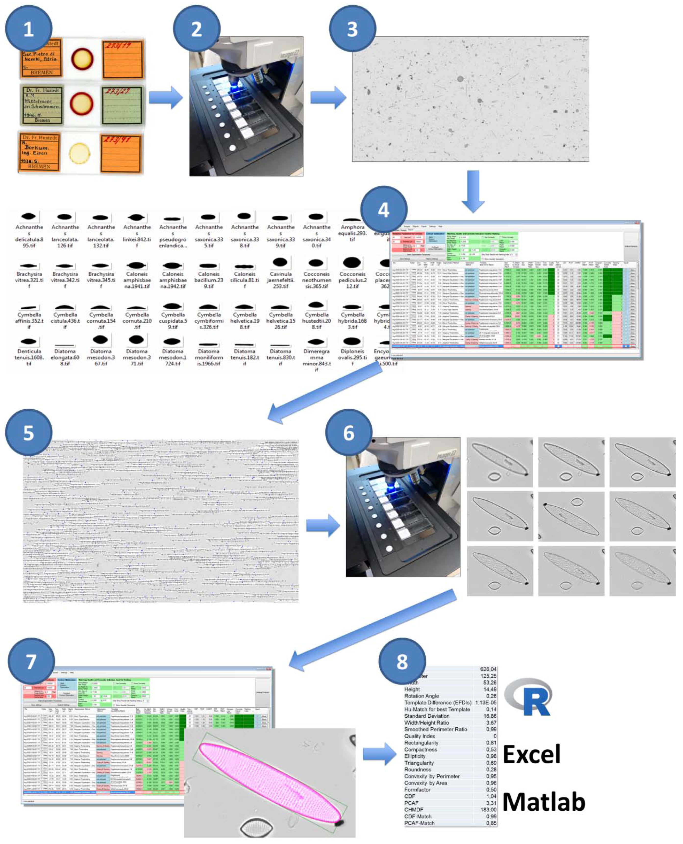
We implemented a complete workflow for semi-automated light-microscopic imaging, measurement and analysis of diatom valves (Figure 1, the numbering refers to the workflow steps as they are described below). Content to be analysed consists of cleaned frustules mounted on permanent slides (step 1); the according raw material can originate from planktonic or benthic samples, sediment traps, sediment cores or cultures. Data collection and processing consists of two cycles of slide scanning and image analysis via SHERPA: The first imaging cycle (steps 2–4) serves the purpose of locating valves of interest at low magnification. During the second cycle (steps 5–7), only these valves of interest are imaged at high magnification and measured at high precision. This method provides a good trade-off between manual effort, time consumption and data economy. Final analysis of the morphometric features measured by SHERPA is realized via R scripts customized to the particular problem (step 8).
For image acquisition, we use a Metafer slide scanning system (MetaSystems, Altlussheim, Germany) operating with a ZEISS AxioImager.Z2 using ZEISS objectives Plan-APOCHROMAT 10x/0.45, Plan-NEOFLUAR 20x/0.5 and Plan-APOCHROMAT 63x/1.4 with oil immersion. Images are obtained with a CoolCube 1m monochrome camera (MetaSystems). In combination with the system’s three-colour (red, green, blue) LED illumination, colour images can be recorded by taking three images of each position and combining them in silico. Since permanent slides prepared of oxidized diatom frustules contain no relevant colour information, we solely use blue LED illumination in all imaging procedures to achieve the highest possible optical resolution.
Regarding diatom analysis, the Metafer slide scanning system is capable of two main modes of operation. In area scan mode, a user defined rectangular or circular region on a slide is imaged in overlapping fields-of-view; these images can be combined (stitched) into large panoramic overview images (virtual slides) using the VSlide software (version 1.1.101, MetaSystems). In position list mode, a list of user-defined positions, spread arbitrarily over the slide, can be imaged. The vertical position of objects can be determined by automatic creation of a focus map, i.e., based on interpolation between reference points, or by autofocusing at each position captured, or using a combination of both. Each object/field-of-view can optionally be photographed at multiple focus depths, and the resulting images can, again optionally, be combined (stacked) to extended focus depth images.
All parameters regarding the operation of the slide scanner are recorded in so-called classifiers. These include settings for illumination (intensity, colour) and imaging (exposition, number and distances of focal planes to image) as well as parameters related to stacking focal plane images. Further settings are related to image post-processing and object detection, the latter of which is unfortunately too simplistic to be useful in diatom analyses; these are not applied in the workflows presented in this contribution. The actual classifier settings for each run are saved alongside the images produced, enabling the reproduction of an imaging run or the transparent application of a standardized set of settings to multiple slides. The only important component of an image acquisition workflow that is not explicitly documented in the classifier archive files is the autofocus settings. Settings for finding the focus are, similarly to classifiers, recorded as named parameter combinations, and the classifier files only record this name. Metafer settings and configuration files, as used in this project, are provided as Supplementary Materials.
Image analysis and object measurement is realized by our software SHERPA (version 1.1c) [5], which is a freely available Microsoft Windows software developed specifically for diatom morphometry. SHERPA can apply a set of different image processing methods for detecting objects in light microscopic images, and compares their contour outline to a set of shape templates to identify objects of interest. An internal rating and ranking system assesses the relevance and quality of results to reduce efforts for reviewing them manually, but nevertheless enables for manual review of objects found and for correction of faulty segmentations which lead to flawed object outlines. All parameter settings can be saved and restored to reproduce the settings. For the selected objects of interest, coordinates with respect to the images they were found in, as well as a wide variety of morphometric feature descriptors, can be exported. The coordinates (in our workflow originating from the low-resolution area scans) can be saved into an XML annotation file which can be read by the VSViewer software (version 2.1.103, Metasystems, Altlussheim, Germany) and subsequently converted into a position list for high-resolution imaging in the Metafer imaging software (version 3.10.4, Metasystems, Altlussheim, Germany). For morphometric analysis, measurements obtained by SHERPA can be exported as CSV files along with cut-outs of the original images and intermediate image processing results. We process this CSV output by R scripts that allow for a quick, easy and flexible analysis of various morphometric descriptors, but, being simple comma-delimited text tables, they can be viewed and analysed just as well with any other spreadsheet/data analysis software.
The number of parameters influencing the results of an image analysis procedure with SHERPA is substantial. Settings regard the parametrization of pre-processing applied for each of one or more segmentation methods and the optional subsequent contour optimization, the identification of valves of interest, and the filtering, scoring and ranking of results. To ensure transparency and reproducibility, SHERPA supports saving a combination of settings and re-applying it to several image data sets. The according configuration files and templates are provided as Supplementary Materials.
In the following, we describe the workflow illustrated in Figure 1 in detail (the numbering in that figure refers to the workflow steps as they are described below):
Step (1): Preparation
Throughout this contribution, microscopic imaging is performed from so-called permanent slides, prepared by embedding oxidized frustule samples into a mounting medium. Since strong object contrast is vital for successfully automating image processing, we recommend using a high refractive index mountant like Naphrax. Another critical issue is sample density. On the one hand, the density has to be sparse and uniform enough to preferably show objects clearly separated from each other, because overlapping impedes automatic valve detection by SHERPA and thus could increase manual efforts required for selecting and reworking valve shapes. On the other hand, the density has to be high enough for focus map creation to find objects at random positions on the slide. We qualitatively found that optimal sample density for the automated procedure is somewhat lower than that for manual counting.
Step (2): Low-resolution area scan for locating valves of interest
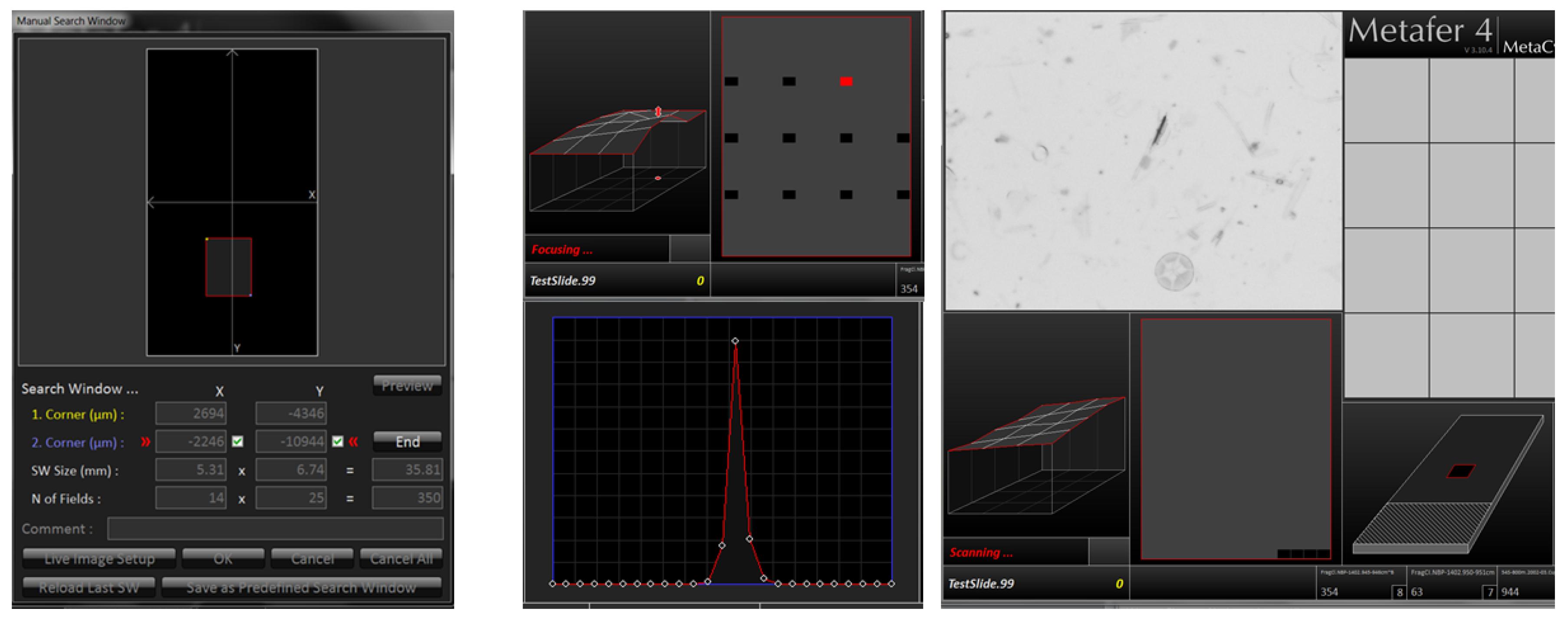
Our two-cycle microscopy and image analysis procedure starts with a low-resolution area scan (see Figure 2), creating a slide overview with a magnification appropriate to the investigated diatom. Usually we employ a 20× magnification objective, with a lamp intensity of 150, in combination with a maximal integration time of 0.011 s. Individual fields-of-view overlap by 64 μm in both X and Y directions. Finding the focus for each image position is performed in two steps: First, at the start of each run, a focus map of the slide is prepared. For this, the optimal focus position is located over a 2 mm grid spanned over the target area by determining the value of a focus function at 25 positions in 5 μm steps and finding the Z position giving the maximum absolute local contrast (focusing mode 0: absolute local contrast, contrast mode 0). Subsequently, the focus map is created by linear interpolation of determined optimal focus Z values over (X, Y), covering the target area. After the focus map is created, the area scan itself is performed by fine focusing at each position, followed by final image capture. For fine focusing, the value of the focus function is determined (focusing mode 2: horizontal quadratic normalized gray level distances, pixel distance 2, contrast mode 0), this time in 40 planes in Z-steps of 2 μm. This second, fine focusing step can sometimes be omitted, but it often leads to substantial improvement in the sharpness of resulting images (depending on density and contrast of diatom valves). Finally, images at 10 focus positions in Z-distances of 2 μm are captured and stacked together to extended focus depth images which are saved for further processing. These stacked images represent the input to SHERPA for locating diatom valves, as well as to the stitching procedure to create a virtual slide.
Step (3): Stitching of virtual slides
The overlapping low-resolution images are stitched together to a virtual slide using the VSlide software (Metasystems, Altlussheim, Germany). These virtual slides enable for visualizing the valves of interest as identified and selected via SHERPA in the context of the whole slide (see steps 4 & 5 below) and also for manually adding further positions for the later high-resolution scan (see step 6 below). Although in principle, it is not strictly required to stitch images to a virtual slide at this stage, this is necessary with the imaging system we are using for two practical reasons: First, the object coordinates relative to individual field-of-view images (as recorded by SHERPA) are transformed to coordinates relative to the whole slide scanned at this step. Second, import of positions into a virtual slide is necessary for feeding a list of positions back into the imaging software in the specific Metafer imaging system we are using.
Step (4): Selecting objects of interest for high-resolution scan via SHERPA
For locating and selecting valves of interest, the low-resolution images (step 2) are processed by SHERPA. Object outlines are compared to a user defined set of shape templates, in case of the example analysis explicated below to the F. kerguelensis templates provided with SHERPA. The template set selected defines the taxonomic scope (more precisely, the scope in terms of outline shapes) of an analysis. Hereby analyses focusing on a narrow range of outline shapes are possible, like in our example application, as are analyses targeting a broad diversity of diatom shapes. For the latter purpose, SHERPA provides a set of ca. 500 outline templates covering a broad range of diatom shapes, which can be further extended by the user to match the specific set of taxa of interest from a particular habitat. Shape optimization and manual corrections are usually not applied since this analysis step is used only for localizing valves, not for measuring them. Convexity analysis often fails on low-resolution images, even for species with strictly convex outlines, especially if the image contrast or sharpness is not optimal. Even though we applied it in our example investigation (see below), we recommend not to do so at this workflow step, at the optional expense of increased efforts for sorting out potential false positives manually. To ensure that settings for validation and ranking are comparable to those of the high-resolution scan (like minimum required object area/perimeter), it is important to set the correct magnification ratio (parameter “Micrometer Factor”; also saved in the settings file). Valves of interest are either picked automatically by selecting all results up to (including) ranking index 2, or by manually reviewing and selecting results. Manual selection is generally conducted at least up to ranking index (including) 2, and can be extended up to higher indices if the amount of highest quality results is not sufficient. The position list for the subsequent high-resolution scan (step 6) is exported as a Metafer VSAI file and saved into the same directory and with the same name as the according virtual slide files.
Step (5): Setting up the position list for high-resolution scan
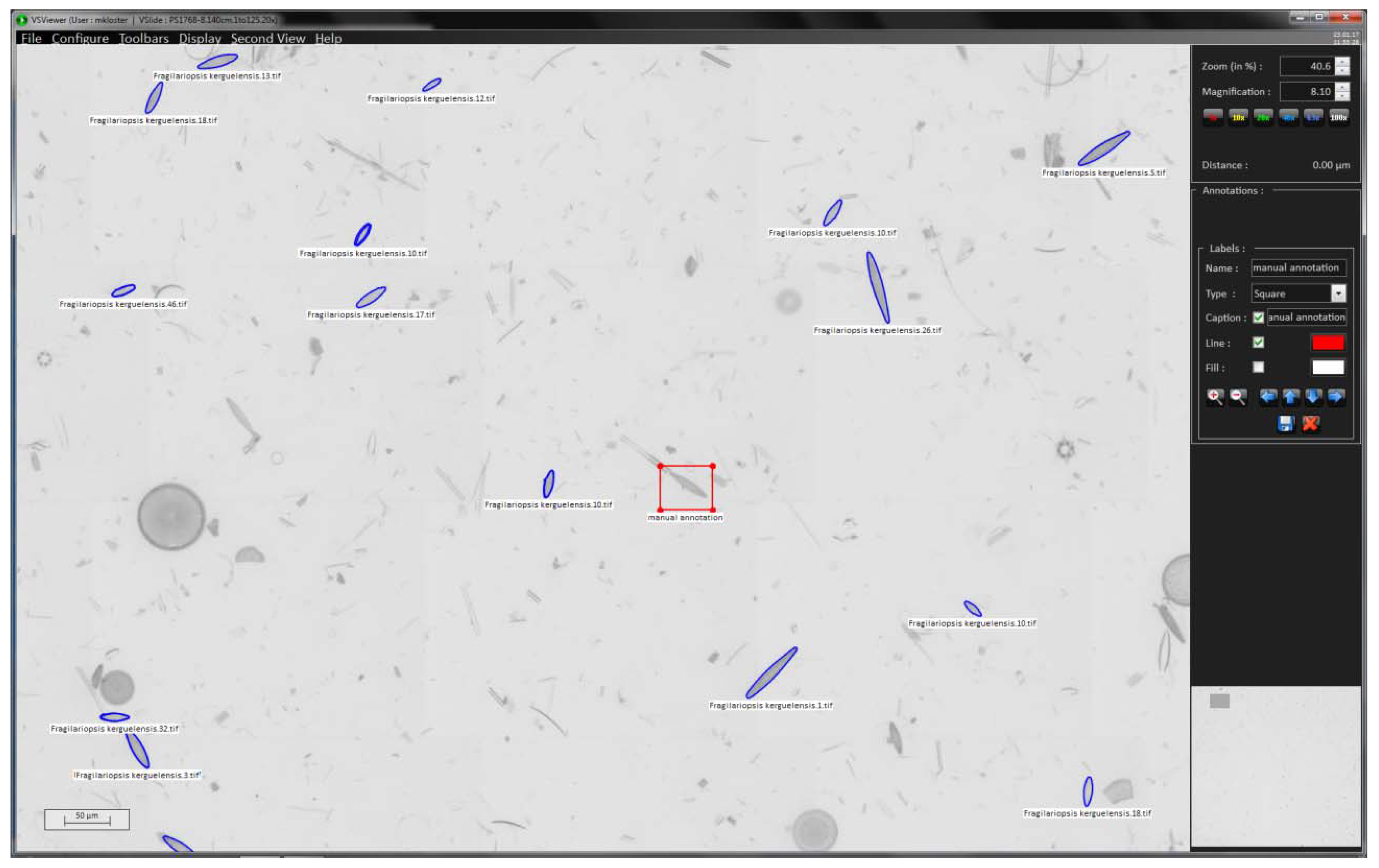
We use the VSViewer software (Metasystems, Altlussheim, Germany) to import the position list provided by SHERPA (step 4) into the virtual slide (step 3), using the “import annotations” function; valve positions are displayed by their annotated outline (see blue markings in Figure 3). The annotation function of the viewer enables to manually add positions of interest if some objects deemed relevant were missed by SHERPA (see red box in Figure 3). This allows for combining (semi-)automated and manual selection of valves of interest.
Step (6): High-resolution position scan of selected objects of interest for precise morphometric measurements
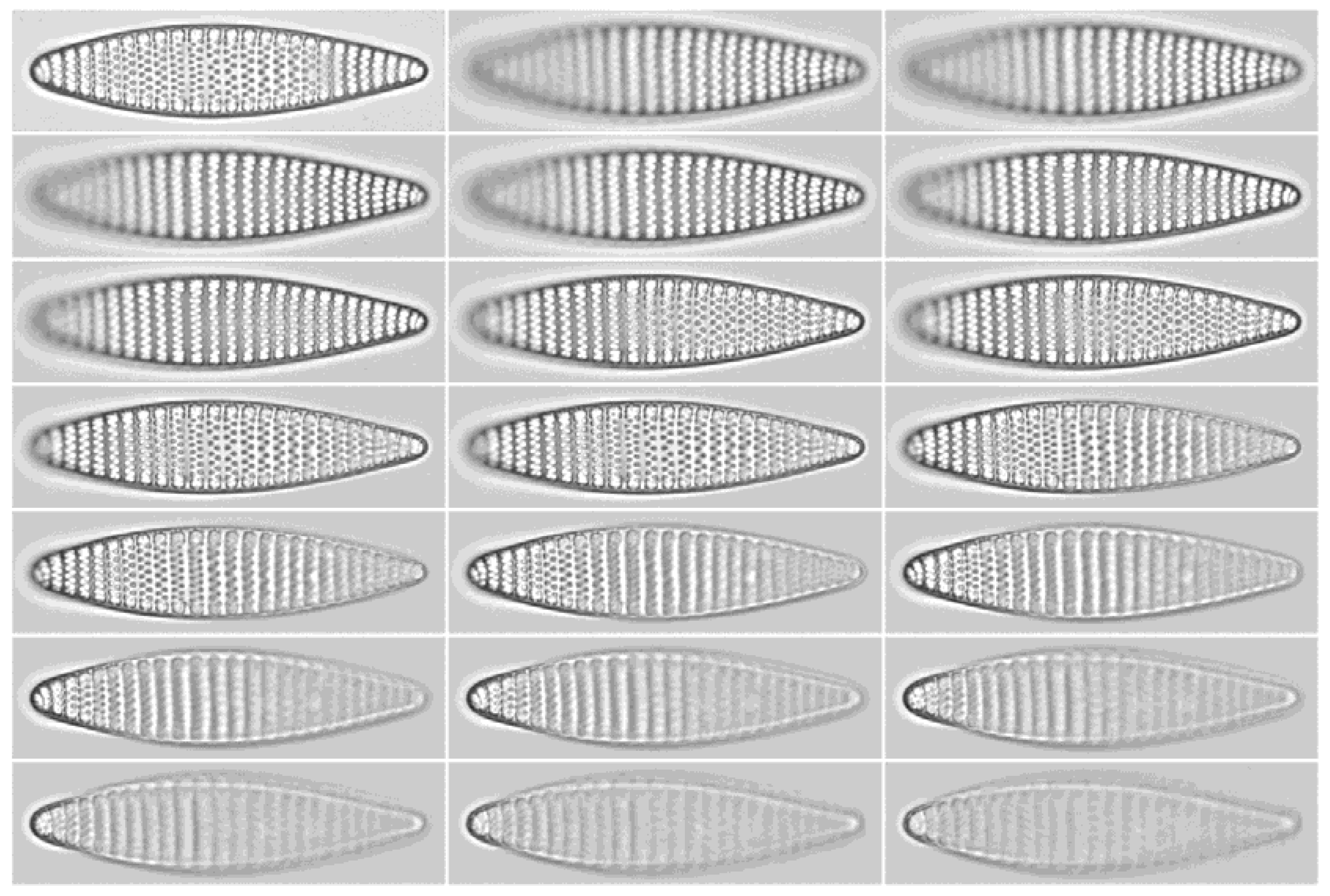
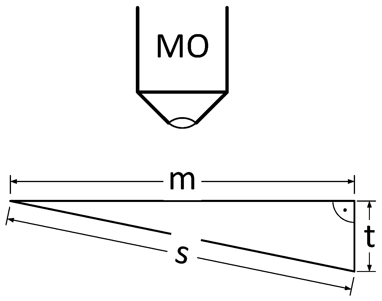
The annotated virtual slide from step 5 contains the (X, Y) position data required for selectively imaging the valves of interest. This high-resolution scan uses the 63× objective with oil-immersion and captures 20 focus levels in 0.2 μm Z-distances after two focusing steps, a first, coarse autofocusing followed by a fine focusing. This is necessary because object positions imported from a virtual slide do not preserve information on the vertical (Z) location of individual objects, so these have to be determined from scratch again. In the first autofocus run, the value of the focus function is determined at 40 Z-positions in 2 μm distances for a coarse determination of the optimal focal plane (focusing mode 2: horizontal quadratic normalized grey level distances, pixel distance 2, contrast mode 0). The focus is narrowed down by a second scan measuring at 60 focus levels in 0.5 μm distances (focusing mode 0: absolute local contrast, contrast mode 0). Subsequently, 20 focal planes around the optimal one are captured in 0.2 μm distances. An extended focus image is produced by stacking the individual focal planes, using the method “CombPlanesFF” with focusing mode 0 and a submatrix size of 128. The individual focal plane images, as well as the extended focus image, can be saved for further processing. In general, for analysis with SHERPA, we only use the extended focus image, since this clearly depicts the valve’s outline as well as its interior ornamentation, even if not all structures can be visualized completely within a single focal plane because of their three-dimensional extent, or because the valve surface is slightly tilted with respect to the focal plane (see Figure 4). Keeping the individual focal plane images leads to a significantly increased demand for storage space, but allows for better manual evaluation of ambiguous species classifications, since in uncertain cases the three-dimensional structure of features, as well as the influence of stacking artefacts, can be judged. The individual focal plane images also allow one to see if a valve lies obliquely, leading to a perspective distortion of its outline shape and size. So far no software is available to make use of this information, but in theory it seems possible to develop automated procedures to correct morphometric measurements for the bias resulting from oblique valve orientation [14]. The maximum possible bias can be estimated according to the Pythagorean theorem (see Figure 5): with s being the actual valve size, m the measured size, and t the tilt. Our setup limits the tilt to a maximum of 4 μm, which results in a maximum error of about 8% for measurements of 10 μm. For larger measurements the error decreases, e.g., for 36 μm, which is the average valve length in our investigation, the maximum error lessens to ca. 0.6%.
Step (7): High-precision measurement of morphometric features from high-resolution images via SHERPA
The high-resolution extended focus (i.e., stacked) images are then analysed with SHERPA to measure the valves of interest. Since the low-resolution position list only sets the central position of the field-of-view, images captured in the second, high-resolution run can also depict objects that are not relevant for analysis, but might be detected by SHERPA. To avoid false positives, manual selection of the final set of valves of interest can be conducted a second time, a process which is massively supported by SHERPA. Usually the same settings and shape templates are applied as for the low-resolution scan, the only difference being the magnification ratio set according to the high-resolution objective, and enabling convexity analysis if this is suitable for the species under investigation (i.e., its valve outline does not contain concave/indented parts). For the example analysis explicated below, contour optimization was disabled and convexity analysis enabled. Like for the low-resolution analysis, manual review and selection of results should be conducted at least until ranking index (including) 2, and may proceed to higher indices. Manual rework for correcting inaccurately segmented valve outlines can be applied if deemed necessary. Selected results can be saved to CVS files along with cut-outs of the original images depicting the valve and intermediate stages of image processing to enable for a later (re-)analysis with other tools than SHERPA.
Step (8): Data export and post-processing
Our workflow can produce duplicate results for objects of interest if some of them are captured on more than one field-of-view images. This happens if a valve of interest lies so near to another one that it is also captured in the image centred on the latter. Removing these doublets is the first important step of downstream analyses. Duplicate objects are identified based on a threshold applied to the summed up distances of basic geometric feature measures like apical and transapical axes length, area, circumference and orientation angle. We implemented this approach to be independent of object coordinates supplied by the Metafer slide scanner, enabling to process data originating also from manual microscopy or other slide scanning systems. The according R function (based on R version 3.2.2 [15]) is supplied in the Supplementary Materials.
3. Results
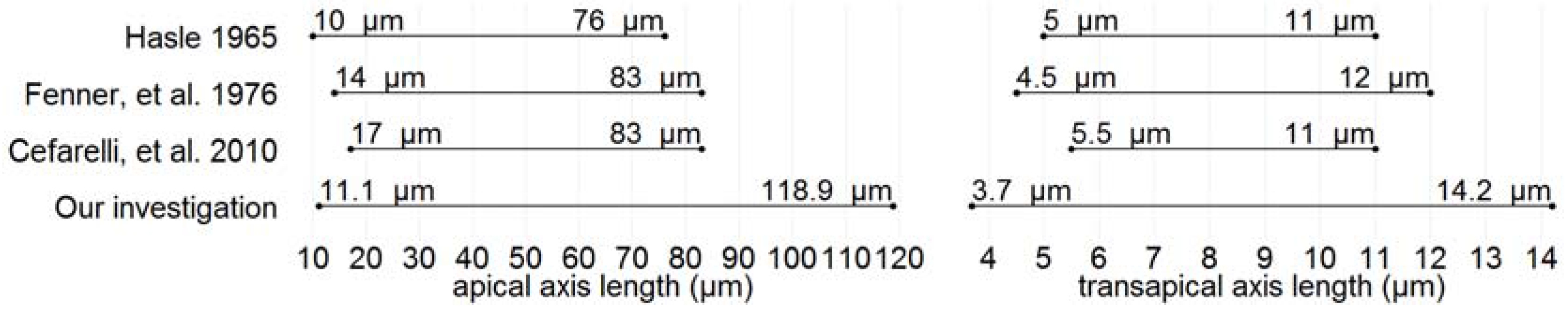
Applying our automated approach, we analysed about 12,000 valves from 72 slides of samples taken from 21 different depths within sediment core PS1768-8 covering marine isotope stadiums (MIS) 1, 2, 5 and 6 (see Table A1). The according CSV file is supplied in the Supplementary Materials. Because this core originates from the central area of the opal belt it consists mainly of diatoms, which are generally well to moderately preserved and do not show significant effects of dissolution on the preserved diatom valves [8]. Our observations substantially expand the size ranges known for this taxon compared to previous reports (see Table 1 and Figure 6).
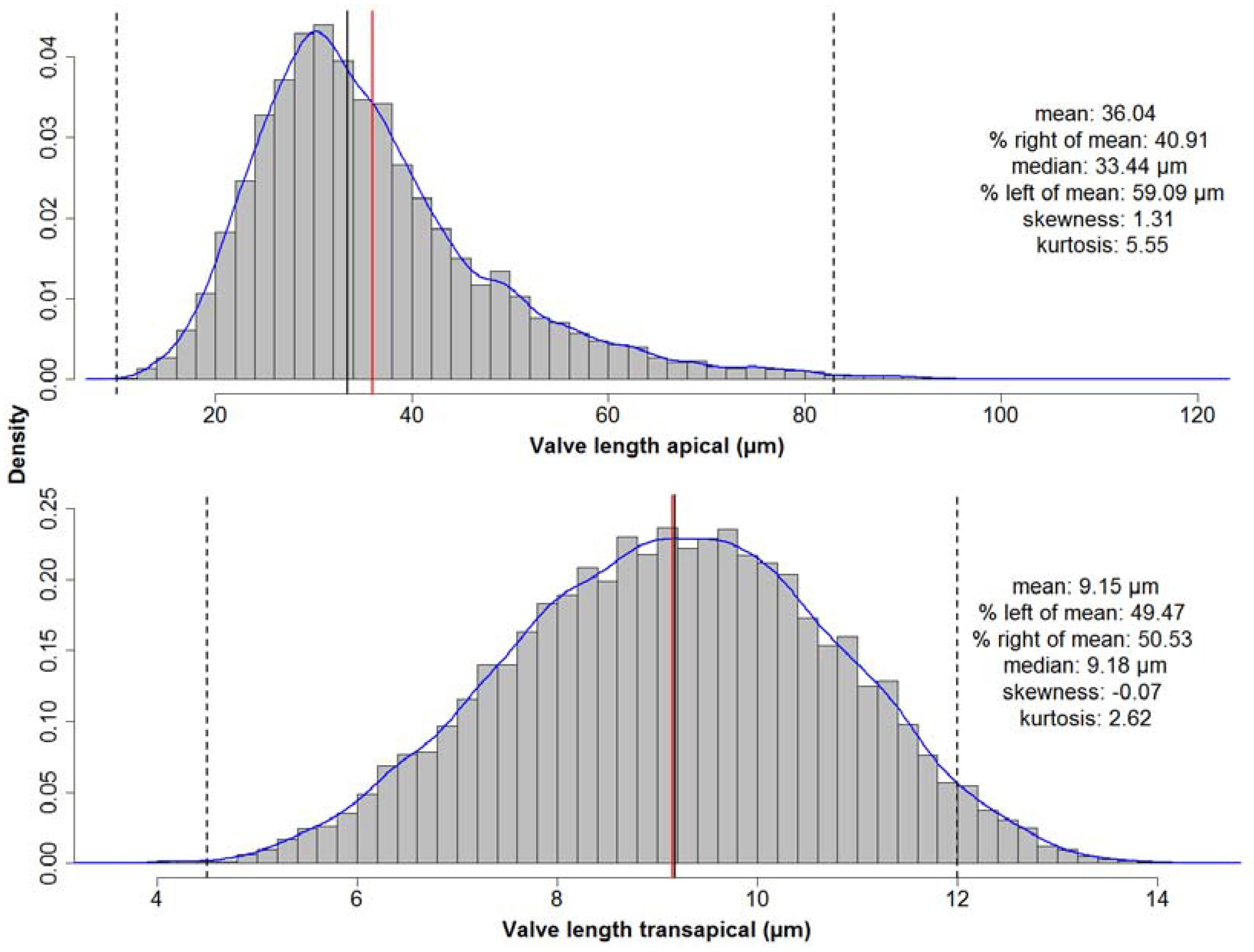
The valves with the longest apical axis were found in the MIS 5 samples. To test whether the species shows a different distribution of apical axis lengths between this and the other MISs, Kolmogorov–Smirnov tests were used (see Table A2 and Table A3). MIS 1 represents the most recent material we analysed and thus the best to be compared to the investigations of [16,17,18]. Between this and MIS 5 the two-sided test did not support a significant difference. This indicates that the occurrence of very large valves is not caused by a general shift in the valve length distribution of the species during MIS 5. The overall distribution of apical axis length is right-skewed (see Figure 7 top). To the contrary, distribution of the transapical axis length is symmetric (see Figure 7 bottom) but platykurtic (test for non-normality; see Appendix C). For individual analysis of each MIS see Figure A1 and Figure A2 in Appendix D.
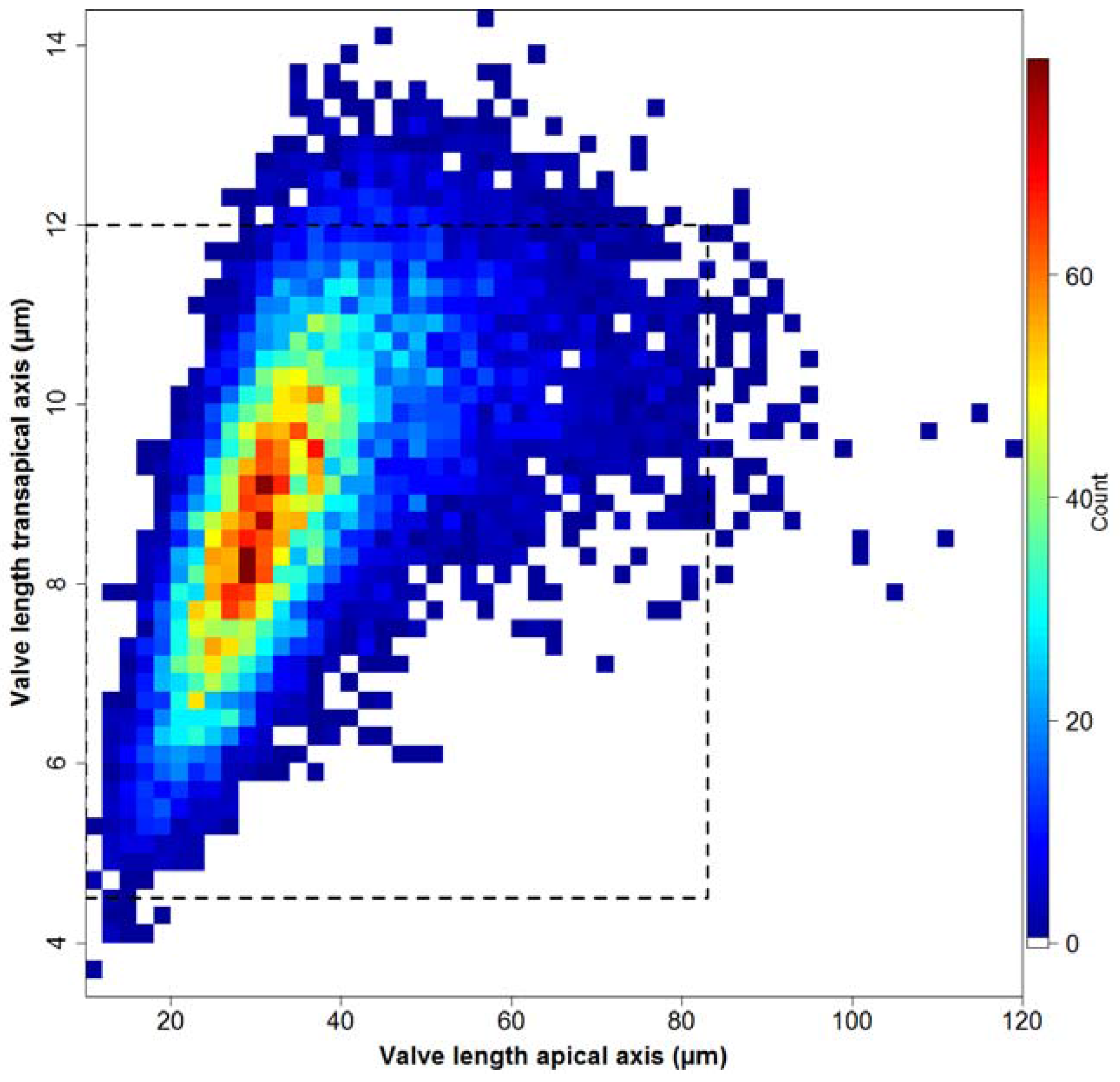
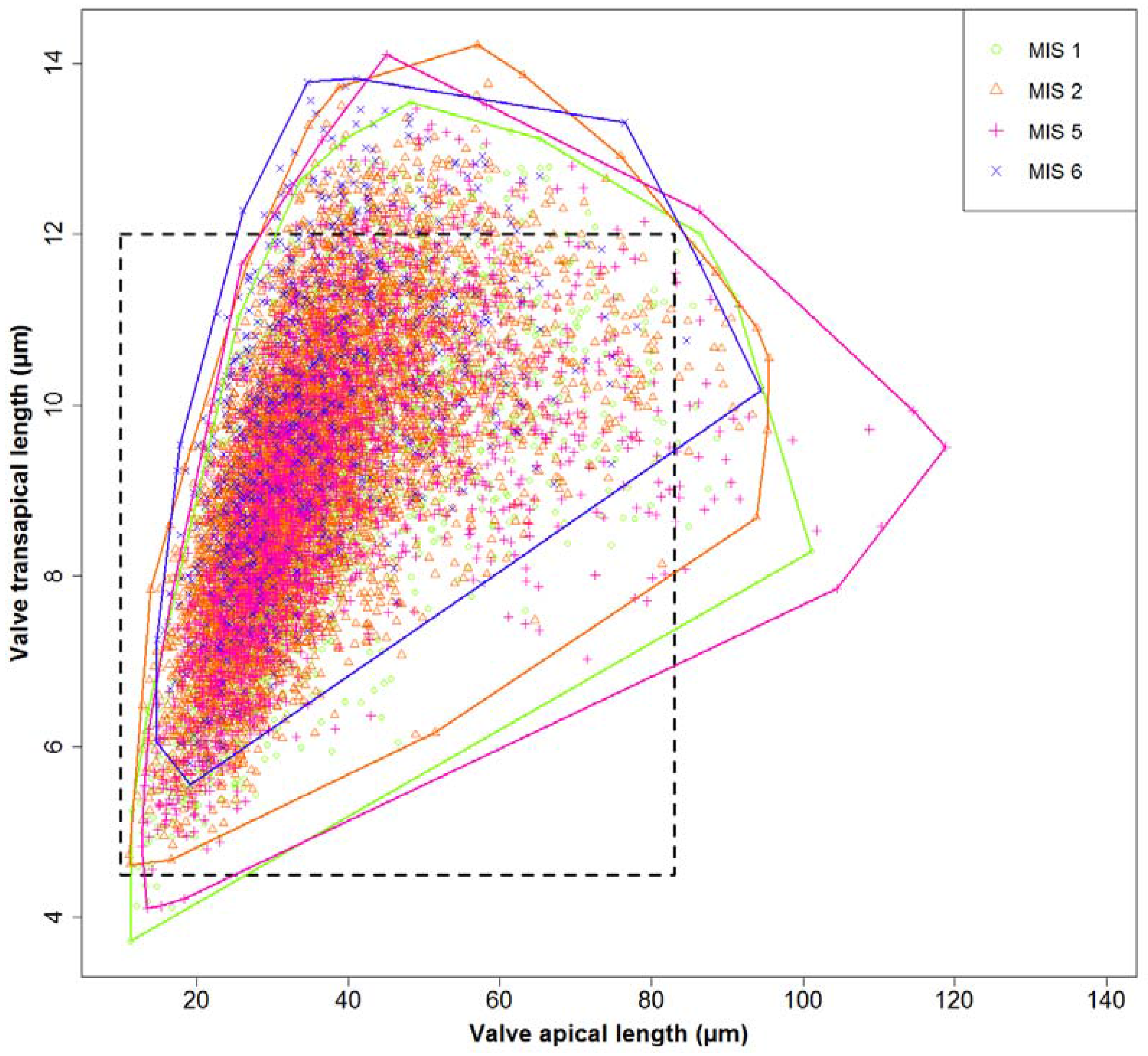
Ca. 5.4% of all valves (505 in total) are sized outside the dimensions reported in the literature [16,17,18], depicted by the dashed rectangle in Figure 8.
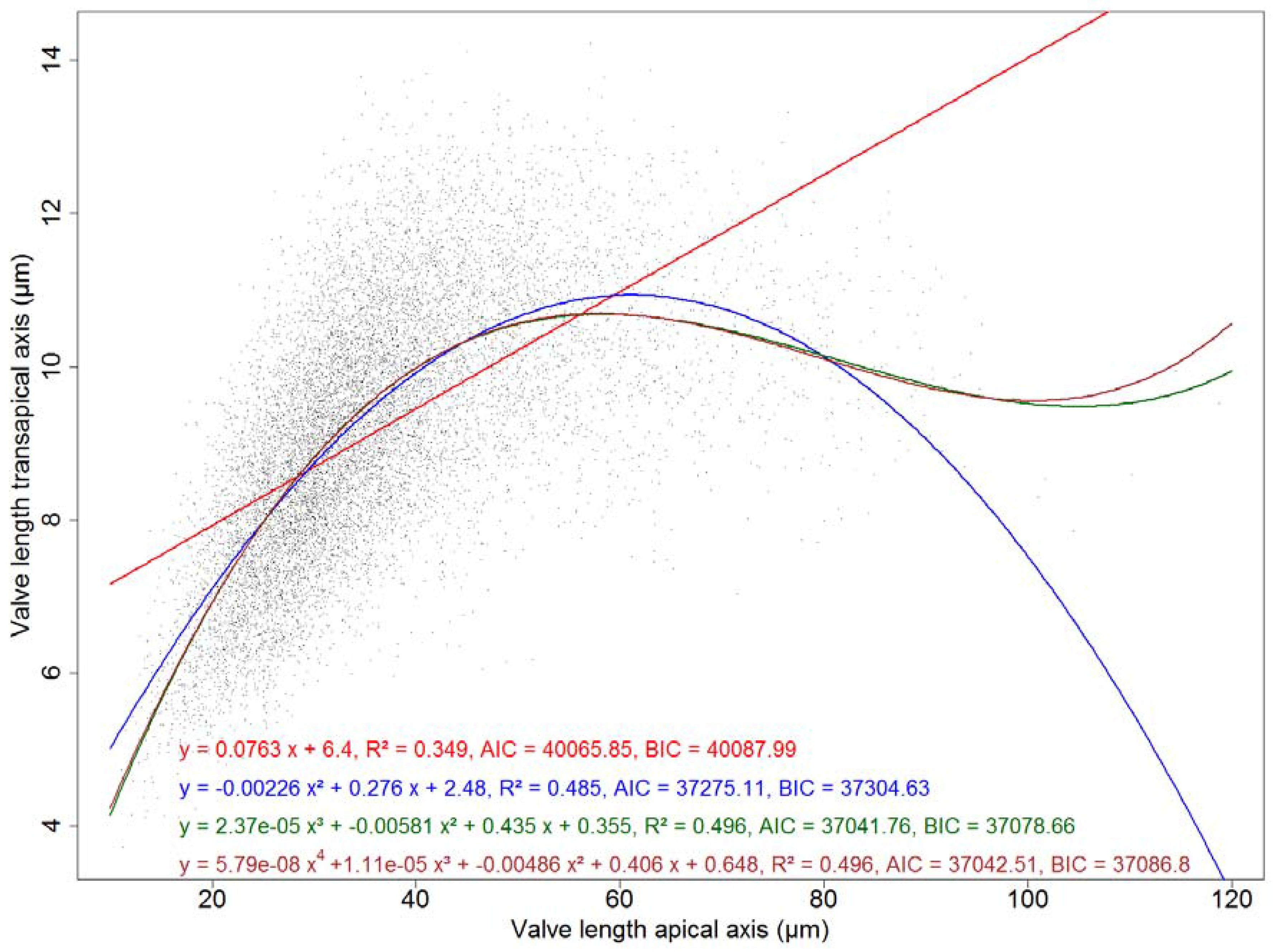
We modelled the relationship between transapical and apical axis length using linear models with an increasing order of polynomial terms (see Figure A3). A third-order polynomial gave a better fit (with a R2 of 0.496) than a first- or second-order regression, and lowest values of the Akaike resp. Bayesian information criteria. Adding a term of order 4 did not significantly improve the model fit. This means that, in spite of what might be suggested by the symmetric distribution of transapical valve measurements (see Figure 7, bottom), the transapical tends to increase with apical length only up to about 50 μm valve length. Above this value, the transapical length stays roughly constant or even decreases slightly with increasing apical length.
4. Discussion
Imaging and image processing methods have been developed and spread rapidly for marine research in the recent years [19,20,21,22]. In contrast to many of these techniques, our approach is conducted ex situ on oxidized material, as has been the common practice in diatom research for nearly 200 years. This enables us to combine traditional preparation methodology with recent advances in imaging and automation, and the application of the latter to existing sets of samples. During the ADIAC project a prototyped automated slide scanning procedure was developed, the main limitation of which consisted of the mechanical parts. Since then, commercial slide scanning systems have become available off the shelf, and advances in camera technology improved the image quality significantly.
Optical resolution: In the last decade, a variety of slide scanning microscopes have become available, which are capable of producing virtual slides by stitching together overlapping field-of-view images. In many biomedical applications, however, a much lower optical resolution is sufficient, and 40× or lower objective magnification is the highest available in many slide scanning systems on the market. For applying to diatoms, however, it is important to select a slide scanning system that can also robustly operate with high-resolution oil immersion objectives. A different high-throughput imaging and measurement method, using unmounted, but still acid-cleaned diatom frustule material, has been proposed previously by [23]. In special settings, like for monospecific cultures, their FlowCam-based method can probably provide a superior throughput compared to our workflow. However, the range of morphometric descriptors seems limited to cell length in the case of the FlowCam. Also, the accuracy of measurements is expected to be higher in the case of images obtained using high-resolution oil immersion objectives from permanent slides, and probably even higher, but definitely more precisely reproducible, than data obtained by time-consuming manual measurement (whether using an ocular micrometer or software-assisted linear measurement between manually selected points in a digital image). The variation of valve measurements induced by using multiple segmentation methods simultaneously in SHERPA is usually around 1% [5].
Focus: Autofocusing at a specified slide position (X, Y) is realized by capturing images at different focus depths (Z), determining the value of a focus function at each Z position and finding the location of its maximum. The focus function used, the Z-range captured, as well as the steps size, can be controlled by the user. Finding the best focus position is a low-level component of the imaging workflow that is applied at a number of different steps throughout, and autofocus settings for different steps (focus map creation vs. final imaging) and for different objectives need to be optimized separately.
An area scan consists of a number of steps (see Figure 2 for a graphical overview): After selection of the target area, the Z position providing the maximum of a focus function is determined over a grid covering the target area. Using linear or spline interpolation, a focus map is created estimating the height (Z coordinate) of the optimal focus position across the whole target area. The way the focus grid is created can be controlled by the user in fine detail. Respective parameters regard the resolution of the grid for focus map creation, the autofocus settings applied in this step, as well as the interpolation method. The target area is divided into overlapping fields-of-view that are captured one by one. For each (X, Y) position, the Z position can either be determined from the interpolated focus map, or from a renewed autofocusing around that Z position (fine focus).
There are two main reasons why images captured in a single focus position determined from a grid interpolation are often not optimally sharp: first, minute local variation in frustule positions in the Z direction on a preparation often exceeds the depth of focus of even relatively low-resolution (10×, 20×) objectives. Second, in the case of several taxa, relevant morphological information is located in different focal planes across a single valve (for instance, the outline is often best discernible in a different Z position than valve face structures like striation). One of the possible measures to improve this situation is conducting a renewed autofocusing at each image position, which enhances the quality of the resulting images (more homogeneous sharpness), but comes at the cost of increased processing time. Another possible measure to address local variation in object Z positions is to capture and combine an image stack at each (X, Y) position. If this is performed over a range that covers the heterogeneity in Z positions across the slide, the quality of the stacked images can be comparable to or even better than those captured after renewed autofocusing even if a second autofocusing step is omitted. The trade-off for this measure is a substantially increased processing time. In our experience, however, it is difficult to estimate in advance the degree of Z position heterogeneity before a scan. We found, therefore, that the most generally applicable procedure is to combine a renewed autofocusing with image stacking (as opposed to capturing a single image only at each position). Renewed autofocusing ensures that the images are taken in a Z-range that fits the object height distribution in the specific field-of-view. On the other hand, capturing and combining images at multiple focus depths ensures that differences in object height within a single field-of-view do not lead to only those objects being pictured sharply which dominate the autofocus function in that field of view (which can be the largest or the most contrasting objects and are not necessarily the object of interest). Focus stacking also improves single-specimen images in the sense that features of the valve lying in different focus depths (for instance, valve outline as well as valve face) are visualised sharply, although in the case of diatoms with complex three-dimensional valve structures, this might create disturbing artefacts.
We note that it is not necessary to combine (stack) images taken at different Z but identical (X, Y) positions into an extended depth-of-focus image. It is also possible to keep the individual Z-position images and analyse them separately or in a combined manner in downstream processing. However, we currently do not see that this could lead to an improvement in the quality of the low-resolution area scan analysis, and so decided to only keep the stacked images for further processing in this case, which helps saving disk storage space. In the case of high-resolution images, we see a strong potential in analysing image stacks as opposed to stacked extended depth-of-focus images, but development of methods specifically suited to the former is substantially more challenging than analyses of stacked images and currently is not part of our workflow.
Investigated Features: During the ADIAC project, a large variety of morphometric features (e.g., Gabor features or Legendre polynomials) were measured and classified for taxonomic identification of diatoms, utilizing a compilation of mostly prototyped methods. In contrast, SHERPA investigates less and partly different features (e.g., elliptic Fourier descriptors [6]) and focuses on finding, imaging and measuring diatoms based on their shape as part of a routine workflow for morphometry purposes.
Data economy: An area scan, as described above, can in principle be performed with any user-selected objective, including oil immersion objectives. Accordingly, it would be thinkable to design an imaging/image analysis workflow where diatom slides are scanned over their whole area using a high-resolution oil immersion objective directly. This is indeed possible (and we have tested the procedure) but causes two difficulties: One is an enormous increase in storage capacity required to save the images. To capture the same physical surface area of a slide, roughly 10 times as many images captured by a high-resolution 63× objective are necessary when compared to a 20× objective. The difference is almost 40-fold when comparing the 63× with a 10× objective. In addition, the probability of individual diatom frustules not being captured fully on any single field-of-view image increases, hampering downstream analyses. This can in principle be helped by increasing the overlap between neighbouring fields-of-view, but to ensure that most frustules are captured fully in at least one field-of-view, the overlap between neighbouring images should be in the range of the size of the largest frustules in a sample, which is substantial. Taking 64 μm, a not uncommon diatom size, as an example (this matches the overlap between neighbouring fields-of-view in our 20× pre-scan): this corresponds to around 627 pixels in images captured at 63× objective magnification. A full field-of-view image has 1360 × 1024 pixels, i.e., the necessary overlap would correspond to almost half the image width and over 60% of image height. This leads to a further substantial increase of storage capacity, due to the fact that more images are required to capture the same slide area. Besides an increase in storage space requirements by more than an order of magnitude, processing time for downstream steps is also increased in a similar manner.
Due to these complications, we finally adopted a two-step imaging procedure which was previously suggested and tested by the ADIAC project [4]. This consists of a low magnification area scan, followed by an image analysis step locating diatom frustules in the images, and by a high-resolution multiple focal planes imaging limited only to slide positions where objects of interest (frustules) were located (see Figure 1 steps 2–6). This procedure keeps storage space requirements relatively low while still allowing high precision of morphometric characterization. In order to be able to implement this workflow, software functionality for exporting outline point coordinates of objects found from SHERPA and importing these into virtual slides in the VSViewer software was developed in communication with Metasystems GmbH.
User efforts: By all efforts at automation and supporting high throughput analyses, the quality of final results from this workflow can be substantially improved by human intervention at multiple steps of the workflow. Although in some situations it can be satisfactory to receive a subsample of diatom valves of interest in a defined slide area, there are also use cases when it is important to not miss (m)any objects of interest (quantitative counts). Also, diatom valves representing taxa of interest cannot be differentiated from other species (in the case of taxon-specific analyses), and from other types of objects commonly occurring on diatom slides (like sediment particles or unidentifiable fragments of broken diatoms) at a 100% accuracy and specificity. Furthermore, segmentation can be misled by touching or overlapping objects, minor fractures in valves or other anomalies. The workflow using slide scanning and SHERPA allows a fine scale control to address these issues. After the first slide scan generating an overview at low objective magnification, the target objects located by SHERPA can be manually checked and remaining non-diatom objects sorted out before further processing. In SHERPA, one can either use stricter quality settings to speed up or completely skip manual processing and to reduce the number of non-diatom objects detected at the price of perhaps missing more valves of interest; or use more permissive quality criteria potentially allowing a higher yield at the price of more false positives (requiring more processing time to remove these manually).
If it is critical not to miss any valves lying in the slide area of interest, there is a possibility for manual interaction with the virtual slide once object positions and outlines detected by SHERPA have been imported into it. At this stage, the virtual slide can be scanned visually and diatom objects missed by SHERPA can be marked manually in addition so that they are also imaged at high resolution in the next step.
Finally, to improve segmentation results in the case of individual problematic valves (e.g., ones overlapping with other objects), a manual correction of outlines is possible at the stage of SHERPA analysis of high-resolution images. The morphometric features, as well as quality scores and ranking of the object, are updated immediately after such manual corrections, and the fact that a manual correction was applied to the object is recorded in the results table exported by SHERPA for further processing. Again, a decision as to whether a manual processing at this step is sensible and how much time to invest in it can be decided case by case based on the purpose of the investigation.
Practical example: To give a simple demonstration of the workflow introduced, we presented a basic morphometric characterization of Fragilariopsis kerguelensis, one of the most common diatom species in Southern Ocean sediments from the late Pleistocene on to present days [24]. The fact that we can substantially extend on the hitherto reported size range of the species (see Figure 9) seems to simply reflect a substantial increase in sample size. Although qualitatively, we see many of the longest valves in samples from MIS5, a Kolmogorov–Smirnov test did not support a significant difference in apical length distributions of this sample from more recent sediment layers. Whereas taxonomic descriptions circulating in the literature might be based on measuring dozens, perhaps up to a few hundred valves [16,18], using the partially automated workflow presented, we could measure about 12,000 valves. Ca. 0.54% (in total 64) of the F. kerguelensis valves analysed had an apical axis length longer than the maximum of 83 μm reported before by [16,17,18]. The longest valve with 118.9 μm apical axis length (see Table 1 and Figure 6) is ca. 45% longer than the maximum reported before. The shortest valve with 11.1 μm apical axis length is smaller than the minimum sizes reported by [18] and [17], but larger than the 10 μm reported by [16]. The transapical axis length ranges from 3.7 to 14.2 μm, compared to 4.5 to 12 μm reported by [17], where 3.66% (in total 434) valves were larger, and 0.08% (in total nine) valves were smaller with regard to this axis than reported before.
Whilst the distribution of apical valve axis lengths is right-skewed (see Figure 7 top), as can be expected based on size reduction accompanying vegetative divisions, the symmetric distribution of transapical valve axis lengths (see Figure 7 bottom) shows that the size reduction somehow is relaxed along this axis for F. kerguelensis. Whereas it could be suspected, based on this symmetric distribution, that transapical valve width might remain constant with size decrease, this is not the case. The observed pattern is rather a roughly linear relationship of transapical width with apical length up to length of around 50 μm, and a constant or slightly decreasing transapical width with increasing length above that. This relation between apical and transapical valve length can be described by a third-order polynomial that explains ca. 50% of the observed variance (see Figure A3). More details of the morphometrics of the species will be presented in a follow-up publication.
5. Conclusions
We describe a partially automated diatom slide imaging and image analysis workflow consisting of commercially and freely available components, making such a procedure widely applicable for routine research. Extending the size range reported for F. kerguelensis (quite substantially, by nearly 45% in the case of apical length) nicely illustrates the advantages of a (semi-)automated approach for microscopic morphometry of diatom valves, primarily that it makes documenting and measuring large numbers of specimens feasible with moderate effort. The method also enables one to flexibly balance throughput/manual effort required vs. quality (specificity/sensitivity of detecting objects of interest). This workflow is still far from a fully automated optical diatom analysis system also capable of taxonomic identification of imaged valves, as envisioned earlier [4]; nevertheless, it implements substantial components and is usable for performing diatom morphometric research already in its current form.
Supplementary Materials
The following are available online at http://awi.de/sherpa: Settings for Metafer4 software, the SHERPA software, SHERPA settings und shape templates, R functions for reading SHERPA output and removing duplicates from each dataset, morphometric data from PS1768-8. The latter one also is available at https://doi.org/10.1594/PANGAEA.873993.
Acknowledgments
This work was supported by the Deutsche Forschungsgemeinschaft (DFG) in the framework of the priority programme 1158 “Antarctic Research with comparative investigations in Arctic ice areas” by grant nr. BE4316/4-1, KA1655/3-1.
Author Contributions
Michael Kloster, Gerhard Kauer and Bánk Beszteri developed the microscopy workflow. Michael Kloster developed SHERPA, and performed the measurements and analysed the data under the supervision of Bánk Beszteri and Gerhard Kauer. Oliver Esper contributed the sediment material. Michael Kloster and Bánk Beszteri wrote the paper.
Conflicts of Interest
The authors declare no conflict of interest. The funding sponsors had no role in the design of the study; in the collection, analyses, or interpretation of data; in the writing of the manuscript, and in the decision to publish the results.
Appendix A
Samples from sediment core PS1768-8.

Table A1.
Information on the analysed samples from sediment core PS1768-8.
| Depth (cm) | Age (years) | MIS | n |
|---|---|---|---|
| 60 | 10,195 | 1 | 85 |
| 80 | 11,182 | 1 | 698 |
| 100 | 12,071 | 1 | 857 |
| 110 | 12,516 | 1 | 553 |
| 120 | 12,960 | 1 | 322 |
| 130 | 13,405 | 1 | 83 |
| 140 | 13,849 | 1 | 255 |
| 150 | 14,912 | 2 | 1659 |
| 160 | 16,130 | 2 | 1458 |
| 170 | 17,347 | 2 | 765 |
| 180 | 18,565 | 2 | 441 |
| 190 | 19,782 | 2 | 650 |
| 200 | 21,000 | 2 | 718 |
| 780 | 119,500 | 5 | 471 |
| 800 | 123,700 | 5 | 437 |
| 810 | 125,800 | 5 | 550 |
| 820 | 127,900 | 5 | 420 |
| 830 | 130,000 | 5 | 732 |
| 840 | 132,100 | 6 | 166 |
| 850 | 134,200 | 6 | 265 |
| 870 | 138,400 | 6 | 274 |
Appendix B
Comparing apical valve axis length distributions from each MIS for significant differences.
Table A2.
The p-values of the two-sided Kolmogorov–Smirnov test show a significant difference between valve apical axis length distributions of MIS 1 & 2, 1 & 6 and 2 & 5 (see bold highlights).
Table A2.
The p-values of the two-sided Kolmogorov–Smirnov test show a significant difference between valve apical axis length distributions of MIS 1 & 2, 1 & 6 and 2 & 5 (see bold highlights).
| MIS 1 | MIS 2 | MIS 5 | MIS 6 | |
|---|---|---|---|---|
| MIS 1 | 1.0000 | NA | NA | NA |
| MIS 2 | 0.0000 | 1.0000 | NA | NA |
| MIS 5 | 0.2808 | 0.0000 | 1.0000 | NA |
| MIS 6 | 0.0429 | 0.1680 | 0.4442 | 1.0000 |
Table A3.
The p-values of the one-sided Kolmogorov–Smirnov test (Alternative hypothesis “greater”) show that the central tendency is greater in MIS 1 compared to MIS 2 and MIS 6, as well as for MIS 5 compared to MIS 2 (see bold highlights).
Table A3.
The p-values of the one-sided Kolmogorov–Smirnov test (Alternative hypothesis “greater”) show that the central tendency is greater in MIS 1 compared to MIS 2 and MIS 6, as well as for MIS 5 compared to MIS 2 (see bold highlights).
| MIS 1 | MIS 2 | MIS 5 | MIS 6 | |
|---|---|---|---|---|
| MIS 1 | 1.0000 | 0.0000 | 0.1408 | 0.0214 |
| MIS 2 | 0.7994 | 1.0000 | 0.9193 | 0.4559 |
| MIS 5 | 0.3137 | 0.0000 | 1.0000 | 0.2246 |
| MIS 6 | 0.8622 | 0.0841 | 0.7043 | 1.0000 |
Appendix C
The Shapiro–Wilk and the Lilliefors (Kolmogorov–Smirnov) normality tests do not support the hypothesis that the symmetrical distribution of transapical axis length is normal (see R output below).
R console output:
> shapiro.test(fkergdata$Height, 5000)) # -> very low p-value, not normally distributed
   Shapiro-Wilk normality test
data: fkergdata$Height, 5000)
W = 0.99782, p-value = 1.589e−06

> lillie.test(fkergdata$Height) # very low p-value, -> not normally distributed
   Lilliefors (Kolmogorov-Smirnov) normality test
data: fkergdata$Height
D = 0.015253, p-value = 1.72e−06
Appendix D
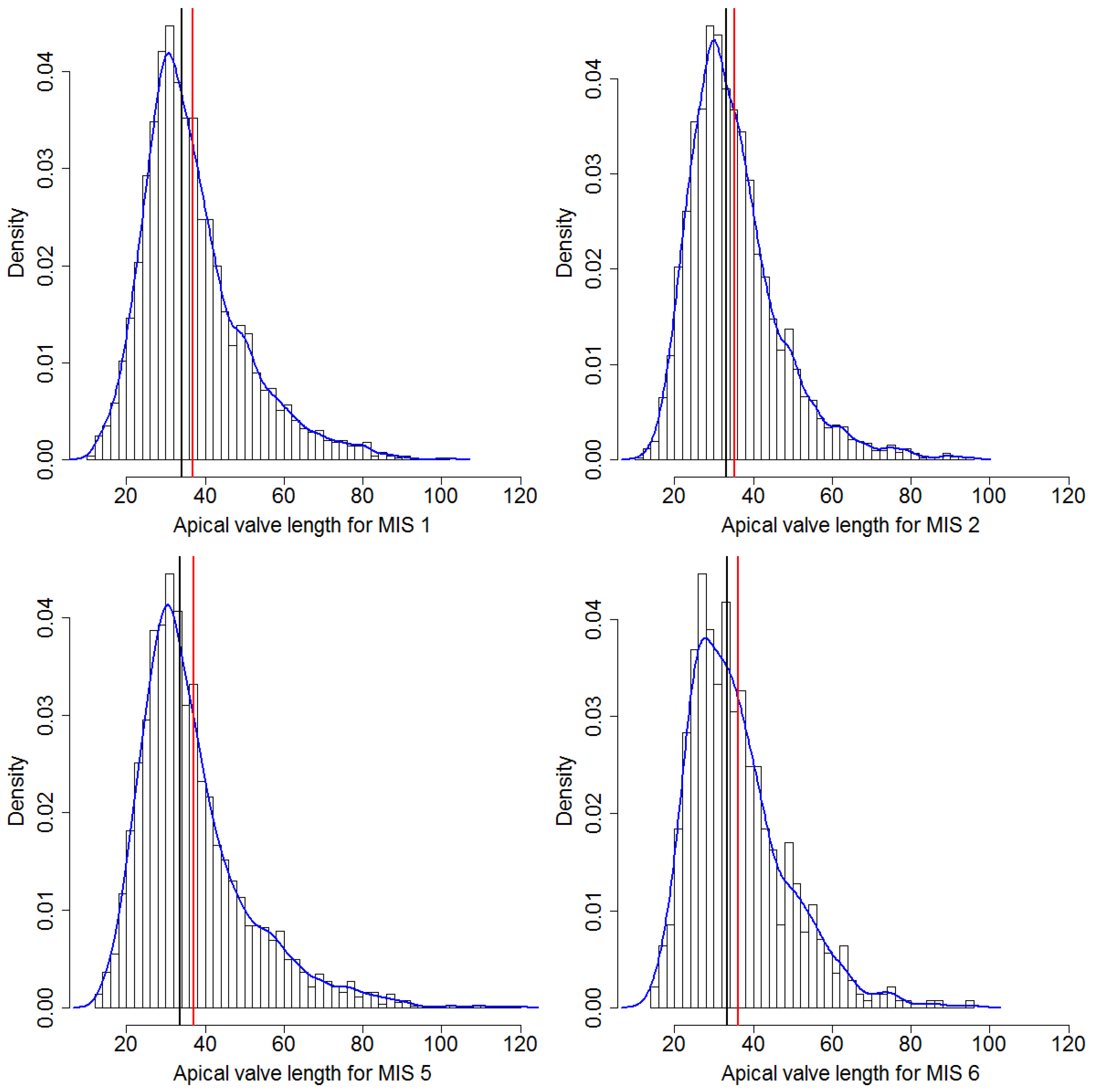
For each MIS we found valves exceeding the size ranges reported before (see Figure A1 and Figure A2).
Figure A1.
Valve dimensions for different sampling depths; coloured lines depict the convex hull around the corresponding data points. Especially during MIS 5, extremely large valves were found. The dashed rectangle depicts the range of valve sizes previously reported in the literature.
Figure A1.
Valve dimensions for different sampling depths; coloured lines depict the convex hull around the corresponding data points. Especially during MIS 5, extremely large valves were found. The dashed rectangle depicts the range of valve sizes previously reported in the literature.

Figure A2.
Distribution of apical axis length for each MIS. Red lines depict the mean, black lines the median values, and blue lines the estimated density curves.
Figure A2.
Distribution of apical axis length for each MIS. Red lines depict the mean, black lines the median values, and blue lines the estimated density curves.
Appendix E
Modelling apical vs. transapical valve axis length. A third-order polynomial gave the best result regarding R2, Akaike and Bayesian information criteria (see the green curve in Figure A3).
Figure A3.
Models of apical vs. transapical valve axis length. The polynomial model of order three (green) gives the lowest value of the Akaike (AIC) and of the Bayesian information criterion (BIC). The polynomial model of order four (brown) does not provide a significant improvement.
Figure A3.
Models of apical vs. transapical valve axis length. The polynomial model of order three (green) gives the lowest value of the Akaike (AIC) and of the Bayesian information criterion (BIC). The polynomial model of order four (brown) does not provide a significant improvement.

1. Statistical assessment of polynomial model order one:
R console output:
> ## modelling valve transapical vs. apical length
> x <- fkergdata$Width # apical axis lengths
> y <- fkergdata$Height # transapical axis lengths
> # poly(1) model
> lmWidthHeightPoly1 = lm(y~x)
> summary(lmWidthHeightPoly1)
Call:
lm(formula = y ~ x)
Residuals:
    Min      1Q  Median      3Q     Max
−6.5225 −0.8975 −0.0182  0.8838  4.7325

Coefficients:
             Estimate Std. Error t value Pr(>|t|)
(Intercept) 6.4029050  0.0365284  175.29   <2e−16 ***
x           0.0762691  0.0009571   79.69   <2e−16 ***
---
Signif. codes:  0 ‘***’ 0.001 ‘**’ 0.01 ‘*’ 0.05 ‘.’ 0.1 ‘ ’ 1
Residual standard error: 1.31 on 11857 degrees of freedom
Multiple R-squared:  0.3488,      Adjusted R-squared:  0.3487
F-statistic:  6350 on 1 and 11857 DF, p-value:  <2.2e−16

> anova(lmWidthHeightPoly1)
Analysis of Variance Table
Response: y
             Df Sum Sq Mean Sq F value    Pr(>F)
x             1  10900 10899.5  6349.7  <2.2e−16 ***
Residuals 11857  20353     1.7
---
Signif. codes:  0 ‘***’ 0.001 ‘**’ 0.01 ‘*’ 0.05 ‘.’ 0.1 ‘ ’ 1
2. Statistical assessment of polynomial model order two:
R console output:
> # poly(2) model
> lmWidthHeightPoly2 = lm(y~ x + I(x^2))
> summary(lmWidthHeightPoly2)
Call:
lm(formula = y ~ x + I(x^2))
Residuals:
    Min      1Q  Median      3Q     Max
−4.5560 −0.8131 −0.0312  0.7789  6.0982
Coefficients:
              Estimate Std. Error t value Pr(>|t|)
(Intercept)  2.481e+00  7.707e−02   32.19   <2e−16 ***
x            2.765e−01  3.668e−03   75.37   <2e−16 ***
I(x^2)      −2.260e−03  4.028e−05  −56.11   <2e−16 ***
---
Signif. codes:  0 ‘***’ 0.001 ‘**’ 0.01 ‘*’ 0.05 ‘.’ 0.1 ‘ ’ 1
Residual standard error: 1.165 on 11856 degrees of freedom
Multiple R-squared:  0.4854,      Adjusted R-squared:  0.4853
F-statistic:  5592 on 2 and 11856 DF,  p-value: <2.2e−16

> anova(lmWidthHeightPoly2)
Analysis of Variance Table
Response: y
             Df  Sum Sq Mean Sq F value    Pr(>F)
x             1 10899.5 10899.5  8035.2  <2.2e−16 ***
I(x^2)        1  4270.5  4270.5  3148.2  <2.2e−16 ***
Residuals 11856 16082.4     1.4
---
Signif. codes:  0 ‘***’ 0.001 ‘**’ 0.01 ‘*’ 0.05 ‘.’ 0.1 ‘ ’ 1
3. Statistical assessment of polynomial model order three:
R console output:
> # poly(3) model
> lmWidthHeightPoly3 = lm(y~ x + I(x^2) + I(x^3))
> summary(lmWidthHeightPoly3)
Call:
lm(formula = y ~ x + I(x^2) + I(x^3))
Residuals:
    Min      1Q  Median      3Q     Max
−4.4314 −0.7984 −0.0278  0.7729  4.3329
Coefficients:
              Estimate Std. Error t value Pr(>|t|)
(Intercept)  3.553e−01  1.576e−01   2.254   0.0242 *
x            4.350e−01  1.091e−02  39.879   <2e−16 ***
I(x^2)      −5.806e−03  2.335e−04 −24.869   <2e−16 ***
I(x^3)       2.372e-05  1.539e−06  15.415   <2e−16 ***
---
Signif. codes:  0 ‘***’ 0.001 ‘**’ 0.01 ‘*’ 0.05 ‘.’ 0.1 ‘ ’ 1
Residual standard error: 1.153 on 11855 degrees of freedom
Multiple R-squared:  0.4955,      Adjusted R-squared:  0.4954
F-statistic:  3881 on 3 and 11855 DF,  p-value: <2.2e−16

> anova(lmWidthHeightPoly3)
Analysis of Variance Table

Response: y
               Df  Sum Sq Mean Sq F value    Pr(>F)
x             1 10899.5 10899.5 8195.52  <2.2e−16 ***
I(x^2)        1  4270.5  4270.5 3211.02  <2.2e−16 ***
I(x^3)        1   316.0   316.0  237.62  <2.2e−16 ***
Residuals 11855 15766.4     1.3
---
Signif. codes:  0 ‘***’ 0.001 ‘**’ 0.01 ‘*’ 0.05 ‘.’ 0.1 ‘ ’ 1
4. Statistical assessment of polynomial model order four:
R console output:
> # poly(4) model
> lmWidthHeightPoly4=lm(y~ x + I(x^2) + I(x^3) + I(x^4))
> summary(lmWidthHeightPoly4)
Call:
lm(formula = y ~ x + I(x^2) + I(x^3) + I(x^4))
Residuals:
    Min      1Q  Median      3Q     Max
−4.4436 −0.7984 −0.0282    0.7705  4.3359
Coefficients:
              Estimate Std. Error t value Pr(>|t|)
(Intercept)  6.478e−01  3.061e−01   2.117   0.0343 *
x            4.064e−01  2.787e−02  14.584  <2e−16 ***
I(x^2)      −4.858e−03  8.820e−04  −5.507 3.72e−08 ***
I(x^3)       1.105e−05  1.146e−05   0.964   0.3350
I(x^4)       5.787e−08  5.190e−08   1.115   0.2649
---
Signif. codes:  0 ‘***’ 0.001 ‘**’ 0.01 ‘*’ 0.05 ‘.’ 0.1 ‘ ’ 1
Residual standard error: 1.153 on 11854 degrees of freedom
Multiple R-squared:  0.4956,      Adjusted R-squared:  0.4954
F-statistic:  2911 on 4 and 11854 DF,  p-value: < 2.2e−16

> anova(lmWidthHeightPoly4)
Analysis of Variance Table
Response: y
             Df  Sum Sq Mean Sq   F value Pr(>F)
x             1 10899.5 10899.5 8195.6842 <2e−16 ***
I(x^2)        1  4270.5  4270.5 3211.0849 <2e−16 ***
I(x^3)        1   316.0   316.0  237.6264 <2e−16 ***
I(x^4)        1     1.7     1.7    1.2432 0.2649
Residuals 11854 15764.7     1.3
---
Signif. codes:  0 ‘***’ 0.001 ‘**’ 0.01 ‘*’ 0.05 ‘.’ 0.1 ‘ ’ 1
References
- Álvarez, E.; López-Urrutia, Á.; Nogueira, E.; Fraga, S. How to effectively sample the plankton size spectrum? A case study using flowcam. J. Plankton Res. 2011, 33, 1119–1133. [Google Scholar] [CrossRef]
- Álvarez, E.; López-Urrutia, Á.; Nogueira, E. Improvement of plankton biovolume estimates derived from image-based automatic sampling devices: Application to flowcam. J. Plankton Res. 2012, 34, 454–469. [Google Scholar] [CrossRef]
- Olson, R.J.; Sosik, H.M. A submersible imaging-in-flow instrument to analyze nano-and microplankton: Imaging flowcytobot. Limnol. Oceanogr. Methods 2007, 5, 195–203. [Google Scholar] [CrossRef]
- Du Buf, H.; Bayer, M.M. Automatic Diatom Identification; World Scientific Publishing Co. Pte. Ltd.: Hackensack, NJ, USA; London, UK; Singapore; Hong Kong, China, 2002. [Google Scholar]
- Kloster, M.; Kauer, G.; Beszteri, B. SHERPA: An image segmentation and outline feature extraction tool for diatoms and other objects. BMC Bioinform. 2014, 15, 218. [Google Scholar] [CrossRef] [PubMed]
- Claude, J. Morphometrics with R; Springer Science + Business Media, LLC: New York, NY, USA, 2008. [Google Scholar]
- Gersonde, R.; Hempel, G. Die Expeditionen Antarktis-VIII/3 und VIII/4 mit FS “Polarstern” 1989 = The expeditions Antarktis VIII/3 and VIII/4 of RV “Polarstern” in 1989; Alfred Wegener Institute for Polar and Marine Research: Bremerhaven, Germany, 1990; Volume 74. [Google Scholar]
- Zielinski, U.; Gersonde, R.; Sieger, R.; Fütterer, D. Quaternary surface water temperature estimations: Calibration of a diatom transfer function for the Southern Ocean. Paleoceanography 1998, 13, 365–383. [Google Scholar] [CrossRef]
- Zielinski, U.; Gersonde, R. Diatom distribution in Southern Ocean surface sediments (Atlantic sector): Implications for paleoenvironmental reconstructions. Palaeogeogr. Palaeoclimatol. Palaeoecol. 1997, 129, 213–250. [Google Scholar] [CrossRef]
- Smetacek, V.; Assmy, P.; Henjes, J. The role of grazing in structuring Southern Ocean pelagic ecosystems and biogeochemical cycles. Antarct. Sci. 2004, 16, 541–558. [Google Scholar] [CrossRef]
- Sachs, O.; Sauter, E.J.; Schlüter, M.; van der Loeff, M.M.R.; Jerosch, K.; Holby, O. Benthic organic carbon flux and oxygen penetration reflect different plankton provinces in the Southern Ocean. Deep Sea Res. I Oceanogr. Res. Pap. 2009, 56, 1319–1335. [Google Scholar] [CrossRef]
- Abelmann, A.; Gersonde, R.; Cortese, G.; Kuhn, G.; Smetacek, V. Extensive phytoplankton blooms in the Atlantic sector of the glacial Southern Ocean. Paleoceanography 2006, 21. [Google Scholar] [CrossRef]
- Cortese, G.; Gersonde, R. Morphometric variability in the diatom Fragilariopsis kerguelensis: Implications for Southern Ocean paleoceanography. Earth Planet. Sci. Lett. 2007, 257, 526–544. [Google Scholar] [CrossRef]
- Kloster, M. Digitale Bildsignalverarbeitung in der Bioinformatik: Methoden zur Segmentierung und Klassifizierung Biologischer Merkmale am Beispiel Ausgewählter Diatomeen. Master’s Thesis, University of Applied Sciences Emden/Leer, Emden, Germany, 2013. [Google Scholar]
- R Core Team. R: A Language and Environment for Statistical Computing; R Foundation for Statistical Computing: Vienna, Austria, 2015. [Google Scholar]
- Hasle, G.R. Nitzschia and Fragilariopsis species studied in the light and electron microscopes. III. The genus Fragilariopsis. Skrifter Utgitt av Det Norske Videnskaps-Akademi i Oslo, I. Matematisk-Naturvidenskapelig Klasse, Ny Serie 1965, 21, 1–49. [Google Scholar]
- Fenner, J.; Schrader, H.; Wienigk, H. Diatom phytoplankton studies in the southern Pacific Ocean, composition and correlation to the Antarctic convergence and its paleoecological significance. Initial Rep. Deep Sea Drill. Proj. 1976, 35, 757–813. [Google Scholar]
- Cefarelli, A.O.; Ferrario, M.E.; Almandoz, G.O.; Atencio, A.G.; Akselman, R.; Vernet, M. Diversity of the diatom genus Fragilariopsis in the argentine sea and antarctic waters: Morphology, distribution and abundance. Polar Biol. 2010, 33, 1463–1484. [Google Scholar] [CrossRef]
- Schulz, J.; Möller, K.O.; Bracher, A.; Hieronymi, M.; Cisewski, B.; Zielinski, O.; Voss, D.; Gutzeit, E.; Dolereit, T.; Niedzwiedz, G. Aquatische optische Technologien in Deutschland. Meereswissenschaftliche Berichte 2015. [Google Scholar] [CrossRef]
- Mullen, A.D.; Treibitz, T.; Roberts, P.L.D.; Kelly, E.L.A.; Horwitz, R.; Smith, J.E.; Jaffe, J.S. Underwater microscopy for in situ studies of benthic ecosystems. Nat. Commun. 2016, 7, 12093. [Google Scholar] [CrossRef] [PubMed]
- Briseño-Avena, C.; Roberts, P.L.D.; Franks, P.J.S.; Jaffe, J.S. Zoops-O2: A broadband echosounder with coordinated stereo optical imaging for observing plankton in situ. Methods Oceanogr. 2015, 12, 36–54. [Google Scholar] [CrossRef]
- Schulz, J.; Barz, K.; Ayon, P.; Luedtke, A.; Zielinski, O.; Mengedoht, D.; Hirche, H.-J. Imaging of plankton specimens with the lightframe on-sight keyspecies investigation (LOKI) system. J. Eur. Opt. Soc. Rapid Publ. 2010, 5. [Google Scholar] [CrossRef]
- Spaulding, S.A.; Jewson, D.H.; Bixby, R.J.; Nelson, H.; McKnight, D.M. Automated measurement of diatom size. Limnol. Oceanogr. Methods 2012, 10, 882–890. [Google Scholar] [CrossRef]
- Cortese, G.; Gersonde, R. Plio/pleistocene changes in the main biogenic silica carrier in the Southern Ocean, Atlantic sector. Mar. Geol. 2008, 252, 100–110. [Google Scholar] [CrossRef]
Figure 1.
Schematic overview of our imaging/image analysis workflow, composed of the following steps: (1) Sample preparation, (2) low-resolution scan for locating valves of interest, (3) stitching of the virtual slide, (4) selecting objects of interest for high-resolution scan, (5) setting up the position list for high-resolution scan, (6) high-resolution scan of selected objects, (7) high-precision measurement of morphometric features, and (8) data export and post-processing.

Figure 2.
Overview of the low-resolution slide area scan procedure (step 2 of the workflow). Left: manual selection of rectangular target area. Centre: focus map creation over a 2 mm × 2 mm grid. Right: focus stack capture in overlapping fields-of-view over target area.
Figure 2.
Overview of the low-resolution slide area scan procedure (step 2 of the workflow). Left: manual selection of rectangular target area. Centre: focus map creation over a 2 mm × 2 mm grid. Right: focus stack capture in overlapping fields-of-view over target area.

Figure 3.
Screenshot of VSViewer showing a subarea of the virtual slide of a 20× scan. F. kerguelensis valve outlines imported from SHERPA are highlighted in blue; additional manual annotations are in red. The positions annotated in this low magnification image are used for the selective high-resolution scans in step 6.

Figure 4.
The extended focus image (top left) clearly depicts valve outline and ornamentation, in contrast to the individual focal planes (anything but top left) it is stacked from. On the other hand, the focal plane images preserve information about the obliquity of the valve that is lost in the extended focus image.

Figure 5.
Measured (m) compared to actual object size (s) for a given tilt (t); MO = microscope objective.
Figure 5.
Measured (m) compared to actual object size (s) for a given tilt (t); MO = microscope objective.

Figure 6.
F. kerguelensis valves of extreme apical axis lengths (101.0 to 119.9 μm). Left: MIS 1, all others come from MIS 5.
Figure 6.
F. kerguelensis valves of extreme apical axis lengths (101.0 to 119.9 μm). Left: MIS 1, all others come from MIS 5.
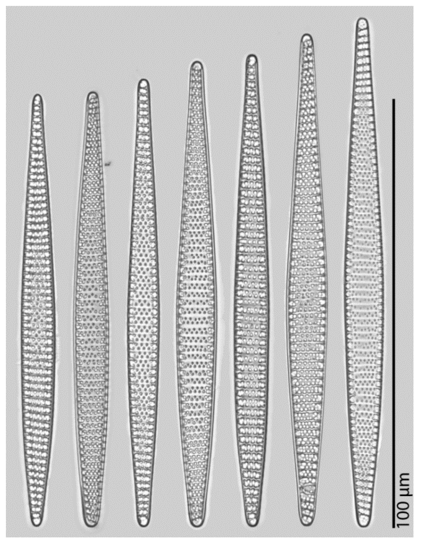
Figure 7.
Distribution of basic valve dimensions along the apical and transapical axes for all MISs. Red lines depict the mean, black lines the median values, and blue lines the estimated density curves. Dashed lines depict the valve size ranges reported in the literature. Whilst for the apical axis the distribution is right-skewed, the distribution of lengths of the transapical axis is symmetrical but not normal (platykurtic, i.e., has thinner tails than a normal distribution).

Figure 8.
Counts of valves of different apical vs. transapical lengths for all MISs. The dashed rectangle depicts the valve size ranges reported in the literature.
Figure 8.
Counts of valves of different apical vs. transapical lengths for all MISs. The dashed rectangle depicts the valve size ranges reported in the literature.

Figure 9.
Valve size ranges reported in the literature compared to our findings.

Table 1.
Summary on F. kerguelensis valve sizes from our investigation. Extreme values are highlighted in bold type.
Table 1.
Summary on F. kerguelensis valve sizes from our investigation. Extreme values are highlighted in bold type.
| Apical Axis Length (μm) | Transapical Axis Length (μm) | ||||||||
|---|---|---|---|---|---|---|---|---|---|
| MIS | n | min | max | mean | median | min | max | mean | median |
| 1 | 2853 | 11.3 | 101.1 | 36.8 | 34.1 | 3.7 | 13.5 | 9.0 | 9.1 |
| 2 | 5691 | 11.1 | 95.5 | 35.2 | 33.1 | 4.6 | 14.2 | 9.2 | 9.2 |
| 5 | 2610 | 12.8 | 118.9 | 37.0 | 33.6 | 4.1 | 14.1 | 9.0 | 9.1 |
| 6 | 705 | 14.8 | 94.4 | 36.1 | 33.5 | 5.6 | 13.8 | 10.0 | 10.0 |
| all | 11859 | 11.1 | 118.9 | 36.0 | 33.4 | 3.7 | 14.2 | 9.2 | 9.2 |
© 2017 by the authors. Licensee MDPI, Basel, Switzerland. This article is an open access article distributed under the terms and conditions of the Creative Commons Attribution (CC BY) license (http://creativecommons.org/licenses/by/4.0/).
Share and Cite
MDPI and ACS Style
Kloster, M.; Esper, O.; Kauer, G.; Beszteri, B. Large-Scale Permanent Slide Imaging and Image Analysis for Diatom Morphometrics. Appl. Sci. 2017, 7, 330. https://doi.org/10.3390/app7040330
AMA Style
Kloster M, Esper O, Kauer G, Beszteri B. Large-Scale Permanent Slide Imaging and Image Analysis for Diatom Morphometrics. Applied Sciences. 2017; 7(4):330. https://doi.org/10.3390/app7040330
Chicago/Turabian StyleKloster, Michael, Oliver Esper, Gerhard Kauer, and Bánk Beszteri. 2017. "Large-Scale Permanent Slide Imaging and Image Analysis for Diatom Morphometrics" Applied Sciences 7, no. 4: 330. https://doi.org/10.3390/app7040330
Note that from the first issue of 2016, this journal uses article numbers instead of page numbers. See further details here.