
Target Tracking Based on a Nonsingular Fast Terminal Sliding Mode Guidance Law by Fixed-Wing UAV

School of Automation Science and Electrical Engineering, Beihang University, Beijing 100191, China
*
Author to whom correspondence should be addressed.
Appl. Sci. 2017, 7(4), 333; https://doi.org/10.3390/app7040333
Submission received: 10 January 2017
/
Revised: 10 March 2017
/
Accepted: 24 March 2017
/
Published: 29 March 2017
Abstract
:This paper proposes a modified nonsingular fast terminal sliding mode (NFTSM) guidance law to solve the problem of ground moving target tracking for fixed-wing unmanned aerial vehicle (UAV) in a planar environment. Firstly, the loitering algorithm is analysed, which can steer the UAV to follow and circle around a ground moving target with the desired distance by heading angle control. Secondly, the effects of different parameters on the convergence time of sliding manifold is presented which is helpful for the designing of sliding manifold. Singularity can be avoided by using a modified saturation function which is obtained through a small range around the null point. Moreover, the NFTSM sliding manifold is used in the loitering algorithm. By using the Lyapunov theory, the finite-time convergence of the proposed method has been proved in the the reaching phase and the sliding phase. In order to verify the approach’s feasibility and benefits, numerical simulations are performed by using a moving target with three different motion states in comparison with the conventional sliding model control method. Simulation results indicate that, under the proposed NFTSM guidance law, the UAV can reach the desired distance in a short time.
1. Introduction
With higher levels of autonomy, unmanned aerial vehicle (UAV) plays an important role in various complex tasks in civilian or military fields [1]. To increase the level of autonomy and reduce the dependencies on manual operators, various planning and control strategies have been developed regarding the problem of target tracking, target acquisition, disaster rescue and so on [2,3,4]. As one of the most complicated and important problems, the target tracking is regarded as a guidance law problem in this paper, assuming the target motion to be observed in the monitoring range. In addition, tracking a moving target by fixed-wing UAV is more challenging than following a predefined path because the target can vary its speed quickly over a large range while the UAV must keep moving forward to stay in the air. Meanwhile, the method for solving the problem of target tracking can be used in the path-following problem by considering the tracked target as a virtual target point on the desired path [5].
When executing the missions such as aerial search or aerial observation, the UAV is often required to orbit around a ground target at a desired distance [6] or maintain the target within a certain distance in front of UAV [7]. Based on the previous studies, the fight strategy for fixed-wing UAV can be divided into a loitering-pattern and following-pattern. Different from the vertical take-off and landing (VTOL) UAV (e.g., quadrotor), the fixed-wing UAV is constrained by the lower bound according to the stall condition. When the target’s speed is lower than the minimum speed of the UAV, the circumnavigation is executed to circle around the target within monitoring range [8]. However, when the speed of the target is close to the UAV, the aircraft should be guided to follow the target by the following pattern.
In previous works, various algorithms have been developed to the problem of target tracking for UAV. The differential geometry is adopted to solve the problem of rendezvous and target tracking guidance laws in [9]. The proposed method has the advantage of rigorous stability as well as less tuning parameters. By implementing Lyapunov vector fields, the guidance laws for unmanned aircraft applications are presented in [10,11]. The vector fields have proven to be globally stable for circular loiter patterns. The concept of Hopf bifurcation is first applied to the standoff tracking problem [12]. It has been verified that the convergent speed of the proposed algorithm to desired distance is faster than the Lyapunov vector field approach. The target tracking problem is studied based on game theory [13]. The control strategy proposed in this study ignores the target’s motion. In addition to the nonlinear control method, the model predictive control (MPC) [14,15], backstepping-based controller [16,17] and sliding mode control (SMC) [18] are presented to get good performance of target tracking.
Due to the existence of the more maneuverable target, the problem of target tracking is more suitable to be solved by SMC so that the feature of sliding manifold can drive the UAV to maintain the desired distance. In order to reduce the effect of unmodelled dynamics and disturbances, the target tracking guidance algorithm is introduced by using SMC based on the tangent vector field [19]. The artificial potentials and SMC are combined to solve the problem of a maneuvering target tracking [20]. A class of the second-order sliding mode for the ground moving target tracking with special unknown bounded uncertainty has been proposed in [21]. In addition, the designed sliding manifold is linear in general SMC [18]. Although the tracking error can converge to zero and the convergence speed can be adjusted by selecting different parameters, it cannot converge to zero in finite-time [22]. The linear sliding manifold can only concern the exponential stability during the sliding phase; as a result, it is difficult for the tracking accuracy to ensure [23].
As aforementioned, this study aims at developing the problem of moving target tracking for the sake of reaching the desired distance as fast as possible. In order to achieve the finite time convergence in the sliding phase, the modified nonsingular fast terminal sliding mode (NFTSM) guidance law, whose sliding mode manifold is a nonlinear function, is applied to solve the problem of ground moving target tracking for fixed-wing UAV in a planar environment. Contrary to the NFTSM technology used in the problem of missile guidance [24], this paper steers the UAV to maintain a desired distance to the target and make the azimuth angle a variable.
The overall structure of this paper is organized as follows: Section 2 mainly introduces the UAV dynamic model and the relative motion model. In Section 3, a modified NFTSM manifold is analyzed and designed. Furthermore, the ground moving target tracking approach for fixed-wing UAV based on modified NFTSM guidance law is proposed in this section. Subsequently, some simulation result analysis is provided in Section 4, and and the conclusions are described in Section 5.
2. Problem Formulation
2.1. UAV Dynamic Model
The vehicle dynamics are based on a simplified flight dynamics model called coordinated flight vehicle (CFV) widely used in most literature [25,26]. The CFV model is described by ordinary differential equations of reasonable complexity, and captures the nonlinear dynamics of maneuvering flight at the same time. We assume that the UAV has a reliable flight control system, which effectively controls the aerodynamic surfaces to accurately track velocity and turn rate commands. Therefore, the UAV’s motion can be simplified on the horizontal plane in the presence of environmental wind, which can be described by the following equations:
where are the UAV’s horizontal position in inertial coordinate system; denotes the UAV’s velocity component in the x- and y-axis, respectively; is the UAV’s heading angle which is the included angle between velocity direction and x-axis; denotes the acceleration command and is the airspeed, which is set to a constant value; and represents the command of heading rate, which is the control object in this paper, with the constraint
For the single-UAV-single-target tracking problem in this study, we suppose that the UAV speed is constant and track the target by holding the altitude constant through the zero climb rate. In addition, is the wind disturbance, and it is easy to get that and , where and denote the speed and the direction of wind disturbance. In the actual application of UAV, the airspeed and the heading angle cannot be obtained easily due to UAV’s scale constraints. For the micro-UAV, the groundspeed and the course angle can be achieved through the external sensors. Therefore, Equation (1) can be rewritten as
the relation between the airspeed and the groundspeed can be constructed as
and the course rate inputs with the restriction can be given as follows:
where
Note that, in the absence of wind, (i.e., ), . From the inequality , we can get that .
2.2. Relative Motion Model
We suppose that the model of the target is similar to the UAV model as shown in Equation (1) with adding the speed command . Namely, the acceleration and turning rate of target are defined as the command for target maneuver strategy. The motion state of target can be summarized as . Due to the fact that the detailed control information cannot be obtained by UAV, the extended Kalman filter (EKF) [27] is utilized to estimate the motion of target in this paper as follows:
where motion state in EKF can be redefined as with and . Therefore, the state equation can be expressed as [28]
where is sampling time. In addition, with is the zero-mean white Gaussian noise, and is the corresponding covariance matrixes. is the variance of . Assuming that the sensor is fixed at the inertial frame origin, so that the observed value can be defined as . is the observed distance between the target and the sensor, while is the azimuth angle. The observation equation in Equation (4) can be given as
where with is the zero-mean white Gaussian observation noise, and is the corresponding covariance matrixes.
Defining the target reference frame by setting the origin of frame at target inertial position, such that the target is relatively static. Figure 1 depicts the relative position between the target and UAV in inertial reference frame and target reference coordinate. The relative motion model between the two vehicles can be described by [29]
where is the desired separation distance between target and UAV; denotes the distance error, where is defined as the distance of two vehicles. In addition, is the auxiliary parameter, and represents the azimuth angle of UAV in the target-frame.
It is noteworthy that the target may flee away from the monitoring range of UAV when the speed of target is greater than the maximum speed of the UAV. Hence, it should be limited in Remark 1 in order to avoid task failure.
Remark 1.
The UAV and wind speeds are assumed to satisfy .
Definition 1.
(Target Tracking Problem) The objective of the target tracking problem is to design the guidance input such that the following conditions are satisfied for the UAV in finite time :
The purpose of the above conditions is to make the status of the tracking system converge in finite time: (i) the distance convergence requires the position of the UAV will merge into the desired distance to the target; (ii) the direction of velocity convergence asks for the vehicle follows an appropriate heading angle (or course angle); and (iii) the convergence of the state ( and will be reached.
3. Target Tracking Based on Sliding Model Control
3.1. Loitering Algorithm
Form the Definition 1, the goal of the target tracking is to keep the distance error as small as possible. However, Equation (5) indicates that there is no direct relationship between the distance error r and the UAV’s heading angular velocity . Consequently, the control strategy should be designed to drive the distance error r to zero. Therefore, it is reasonable to set , namely, . In order to simplify the formula complexity, define , the steady value of can be given by
From Equation (7), the control goal in Definition 1 is replaced as to drive to , such that . In this condition , the distance L reaches its steady state with no changing. Defining the heading angle error is , . By using the trigonometric identities and , the dynamics of the distance error in Equation (5) is rewritten as
Remark 2.
Due to , the inequality is valid when . Therefore, the monotonicity of is the same as the monotonicity of , and is equivalent to .
Hence, one needs to construct a monotonic function satisfying . On account of , we define , for example, as follows
Definition 2.
The target tracking problem defined in Definition 1 can be redefined feasibly as: designing the turning rate to drive the following condition for UAV:
where , while can be controlled directly by .
From Equation (5), factors that determine the relative motion between the UAV and the target include not only distance error rate but also azimuth angle rate . Definitions 1 and 2 just consider r convergence to zero, with as a free variable. The UAV flying circle around the ground target is intuitive when the UAV’s speed is larger than the target’s. In addition, the UAV follows behind the target at the desired distance. Therefore, the UAV is loitering around the target due to the target’s maneuver. The desired position trajectory forming a circle with a radius of divides the plane into two parts. This feature is suitable for using the sliding mode control method, in which the sliding manifold is designed to generate the appropriate circle trajectory for the heading angle to reach control objectives. The next section will apply SMC to design a guidance law to satisfy the conditions in Definitions 1 and 2.
3.2. Sliding Manifold Designing
For the problem of SMC designing, a switching surface providing the desired convergence characteristic should be defined at first. Then, a controller should be designed to steer the objective states to the chosen manifold, which is not influenced by disturbances or uncertainties.
Definition 3.
The conventional terminal sliding mode (TSM) can be described by the following first-order nonlinear differential equation [30]:
where , and is the signum function. s is the sliding manifold.
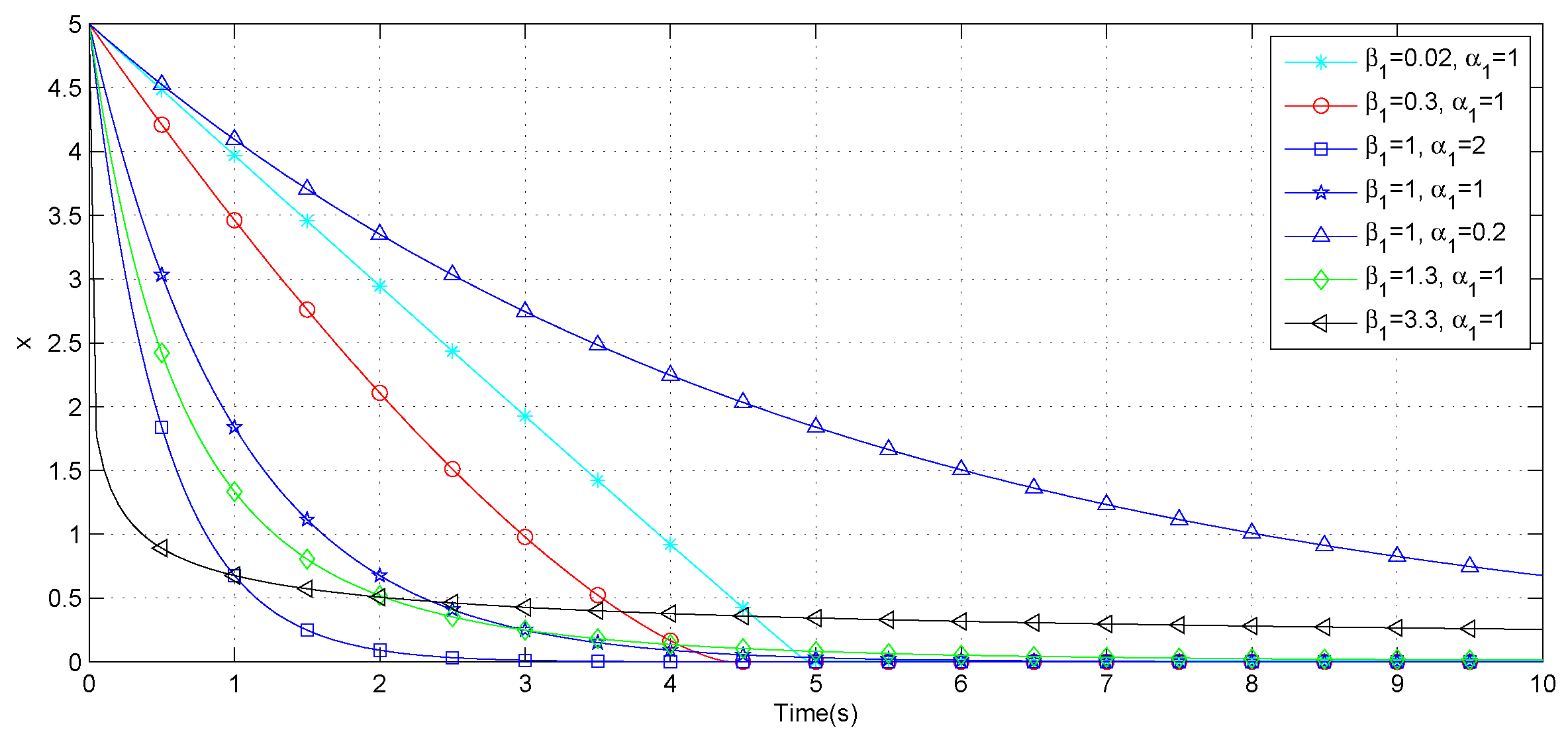
As shown in Figure 2, let the initial state be , and the properties of system (11) can be summed as: (i) when , the system will reduce to , and the system is exponentially stable; (ii) when , the convergence rate increased gradually with the increase in distance from zero. This result is interesting as it can make the system converge in finite-time; (iii) when , the system will converge to origin with a high speed at a distance from zero, but its convergence rate will slow down when close to the origin. The convergence rate is inversely proportional to the distance from zero. In addition for fixed parameters , convergence rate has the same monotony as .
Remark 3.
From the finite-time differential equation, the dynamics (11) are globally finite-time stable with any given initial condition , and the convergence time can be obtained as
As mentioned above, the convergence rate has an obvious difference with different and . It is best to combine the two ways with and . Therefore, the linear combination which is developed as follows not only improves the convergence rate, but is also easy to achieve.
Definition 4.
The fast terminal sliding mode (FTSM) is described by the following differential equation:
From Definition 4, it is evident that FTSM is the combination of different , , and cases. When the system state is far from the equilibrium point, the subitem in Equation (12) dominates , which provides a high convergence rate. However, the main term guarantees the system converge in finite-time when the system state is close to the equilibrium. Therefore, the whole FTSM will converge very quickly. Figure 3 shows that the FTSM has a better convergence rate than the TSM (when ). The result is verified by the following sliding modes setting the initial state :
Remark 4.
The definition of the Gaussian hypergeometric function can be given as follows:
where the beta function is . will keep in Remark 4 convergent, which is demonstrated in [32]. The exact form of varies with the involved parameters. For example,
From Equations (13) and (14), the singularity will occur when and due to , . In order to avoid this problem, the modified nonsingular fast terminal sliding mode (NFTSM) manifold is proposed in Definition 5.
Definition 5.
The NFTSM manifold in this paper can be proposed as follows:
where , , and is defined as
where , , , and η is defined as a small positive constant.
The time derivative of Equation (15) can be expressed as
3.3. Guidance Law
In the subsection, the guidance command is designed for Equation (5) by using the NFTSM manifold given in Equation (15). From Definition 2, the control goal of this study is to regulate to zero. According to Equation (15), we can redefine a new , where , . From Equation (8), the NFTSM manifold s defined in Equation (15) can be designed as follows:
where being a small positive constant. These coefficients , , , , , are gains to be designed.
To make the UAV state quickly converge to the manifold s defined in Equation (17) from the initial states, we select the fast reaching law as follows:
where , and .
From Equation (7), can be expressed as
where according to the hypothesis that the airspeed of UAV does not change.
3.4. Stability Analysis
Lemma 1.
Suppose the continuous positive definite function satisfies the following inequality:
where is the initial time (see [30]). Then, the system converges to the equilibrium point in finite time , and the setting time can be given by
Theorem 1.
Proof.
From [33], considering a Lyapunov function candidate . Applying Equations (17)–(19), the derivative of with respect to time yields
From , is bounded. In addition, Equation (23) can be written as
Equation (24) has a similar form to Equation (21). Consequently, the sliding manifold can be reached in finite time and the convergent time is given by
Case 1: when with , letting the sliding manifold , the equality can be obtained from Equation (17)
Due to , we can then get the inequality as follows:
According to , it is reasonable to set the following inequality:
From Equation (7) and Remark 1, we obtain
Let be a Lyapunov candidate. Applying Equations (8) and (26), on the manifold , the time derivative of can be written as
Consequently, the distance error r will make ℓ converge to the region asymptotically in finite-time. By using Equation (26), we can obtain
Case 2: if , it shows that ℓ will converge to the region in finite-time. By using Equation (17), we obtain
Therefore, we can conclude that will converge to the bounded domain in finite time, which implies that the desired control constraint is held and the state r will converge to zero in finite-time. ☐
4. Simulation Results
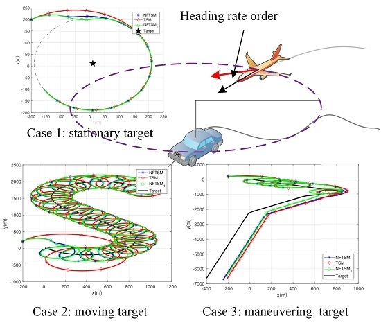
In this section, the numerical simulation results are presented to demonstrate the effectiveness of the proposed guidance law. Three sets of simulations are performed: (1) when the target is stationary; (2) when the target is moving with constant velocity; and (3) when the target is moving with changing acceleration and heading angle rate. These simulations demonstrate successful target tracking capability in all cases. The necessary parameters of target tracking are listed in Table 1.
In order to make full verification for the method in this paper, the proposed NFTSM guidance law is compared with a traditional SMC in [18]. In the traditional SMC method, the sliding manifold can be designed as
In addition, the guidance law is proposed as
where is a high-slope saturation function, which is constructed to eliminate chattering by SMC method, defining as follows:
The coefficients of the NFTSM guidance law proposed in this paper and the traditional SMC method in Equation (35) are listed in Table 2, and another set of coefficients ( and ), not performing good enough, is given as a contrast ().
In this simulation, we get a desired trajectory of the moving target by Equation (1) whose subscript a is replaced as t. In order to simulate the actual situation, we let a virtual sensor observe the information of the target at the inertial frame origin. The motion of the target is estimated by using the EKF. The parameters in Equation (4) can be set as follows: let the sampling time s; set the corresponding covariance matrixes of the process noise and measurement noise are and , respectively. Thus, we can get the estimation of state: .
4.1. Stationary Target
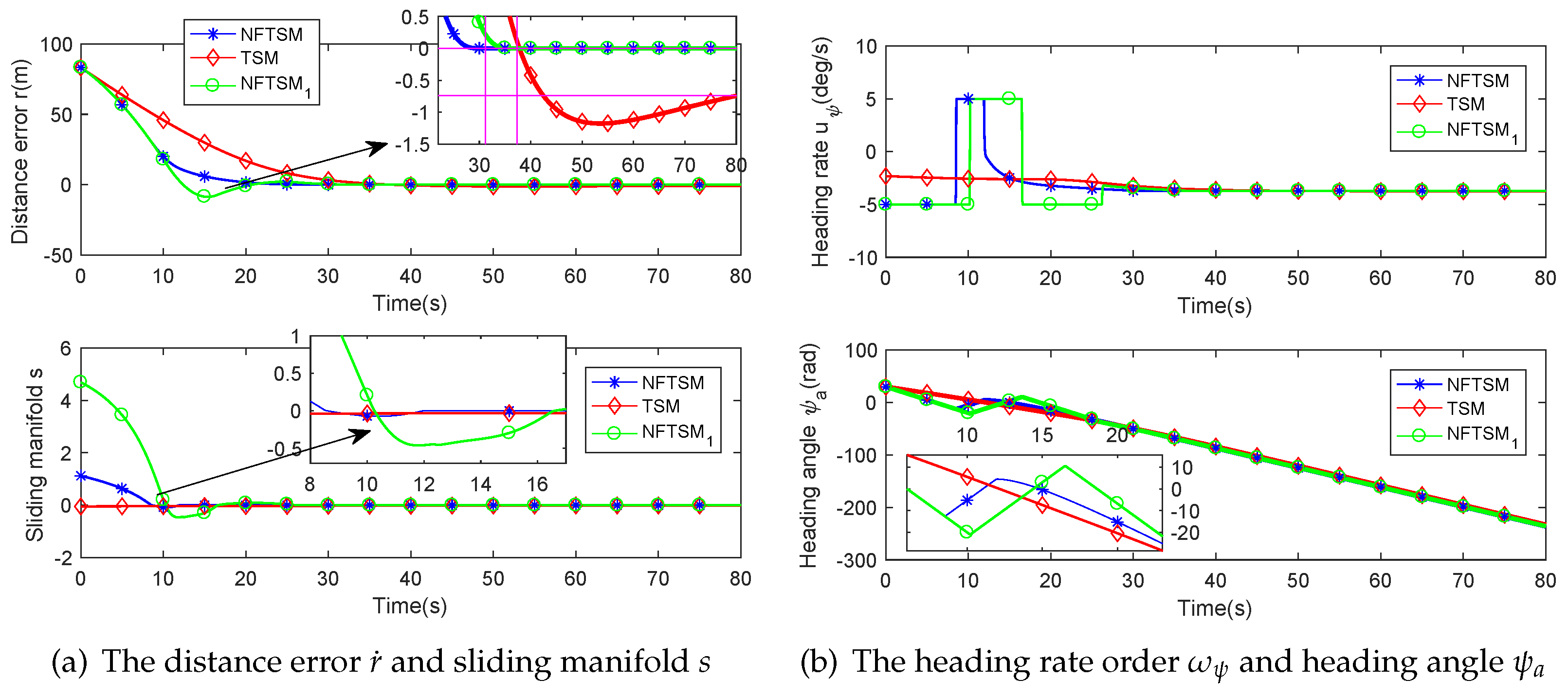
Figure 4 shows the paths of stationary target tracking in the inertial reference frame with different initial heading angle and . For both cases, the distance error , sliding manifold s and the heading rate with the heading angle are shown in Figure 5 and Figure 6, respectively.
From Figure 4a, we can find that all three of the guidance laws will steer the UAV at a constant speed to circle around the target. It is proved that the convergence rate of NFTSM algorithm is faster than the TSM algorithm. However, an overshoot exists when enlarging the and as shown in Figure 5a and Figure 6a, due to the subitem dominating the third subitem defined in Equation (12). This is also the reason why the convergence rate of the TSM algorithm is slower than the others. When , the FTSM is equal to the TSM.
Figure 4b represents that, when the included angle of the the UAV initial heading and the azimuth angle are large, it takes a long time to achieve the desired trajectory for TSM algorithm, but the NFTSM algorithm has reached the goal position in a shorter time already. In Figure 5b and Figure 6b, the heading rate order of the NFTSM algorithm is restricted because it exceeds the maximum UAV turn rate from 8 s to 17 s. In order to obtain quick convergence, the NFTSM algorithm needs a strong mobility, while the TSM algorithm’s result is changing slowly. After closing at the desired position, all three methods can hold the state without divergence because they have the similar third subitem in Equation (12).
Table 3 gives the results of the stationary target tracking. For the case , the distance error r can converge to less than 0.0001 m in 31.2 s by the NFTSM algorithm, while closing at −0.742 m by the TSM algorithm. Because of the existence of shock, the algorithm will converge in 37.3 s. For the case , due to adjusting the course from the large angle, the NFTSM algorithm will converge in 72.9 s, but the other two methods cannot converge in the 100 s simulation time. For the simulation of stationary target tracking, it can be obtained that the proposed algorithm is preformed better than the TSM in convergence time, and the reasonable design parameters are needed to eliminate the shock.
4.2. Constant Speed Target
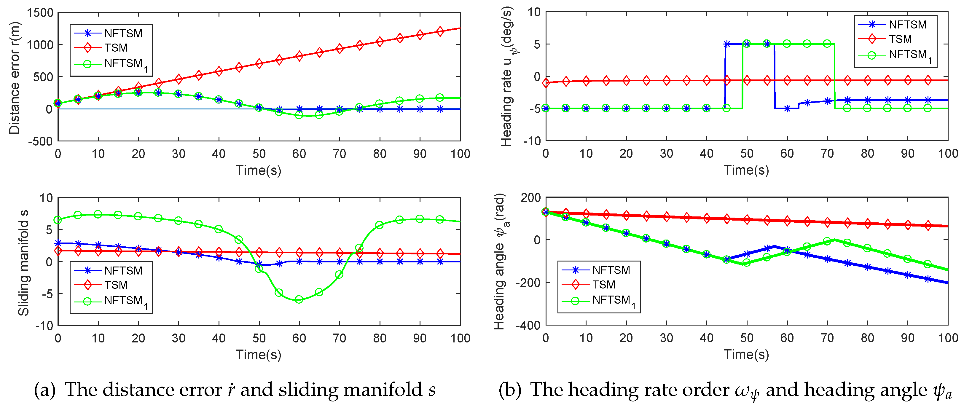
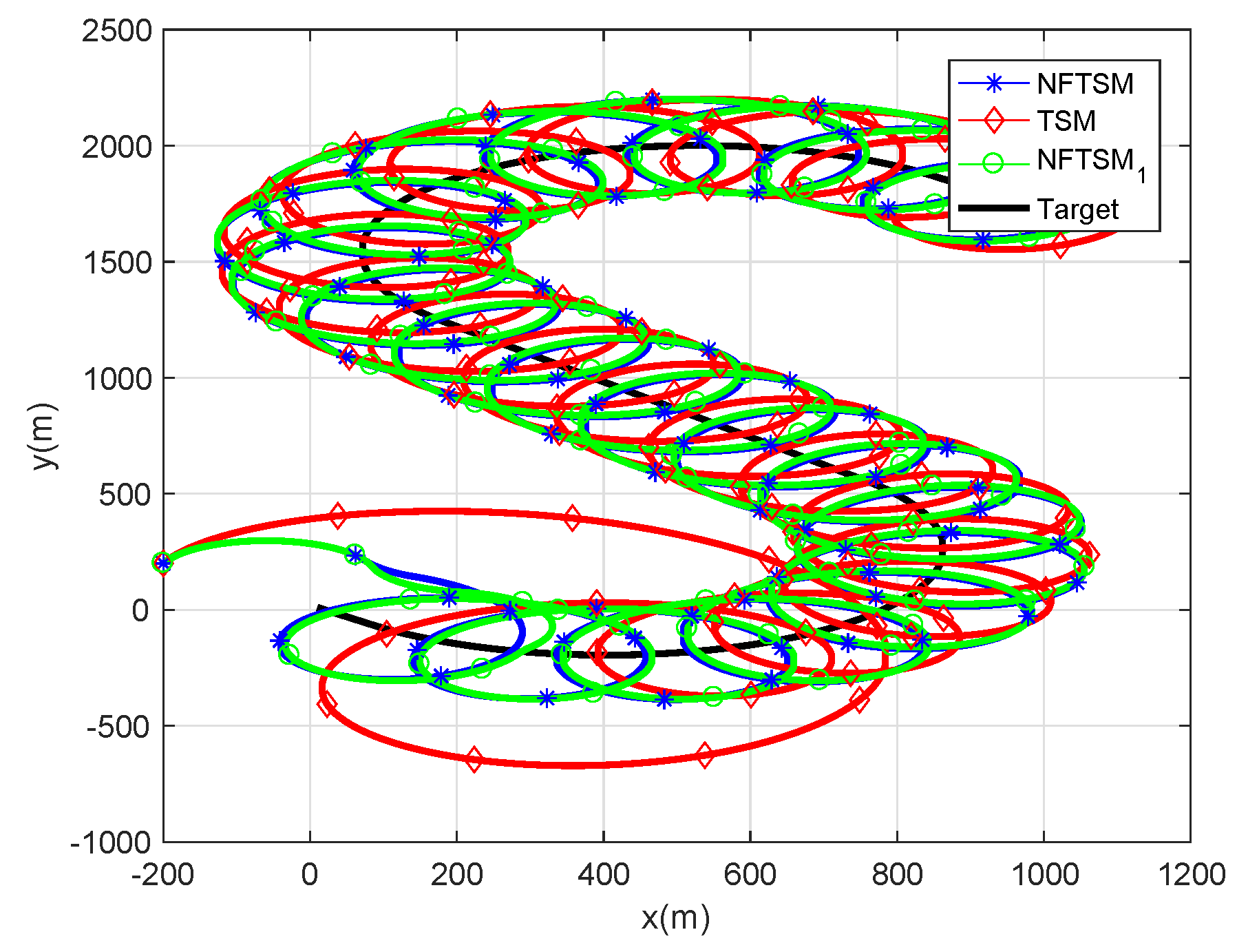
Let the target move following an S-shape trajectory in the barrier free environment with the initial heading angle and the constant speed m/s. The UAV’s initial heading angle . After 2000 s simulation time, we get the trajectories which are depicted in Figure 7. Getting the similar results as the stationary target tracking: the NFTSM algorithm has better convergence rate than the TSM algorithm.
Combined with Figure 7 and Figure 8, we can find that the TSM algorithm has a slow heading adjustment compared with the NFTSM algorithm. The overshoot still exists by at the start state, but it is improved after 75 s. Due to and the azimuth angle being considered as free variables, the UAV can loiter above the target to keep the predetermined distance.
The simulation time of this constant speed target tracking is 2000 s. As is shown in Figure 8a, we can find that all three of the methods will converge to zero in finite-time. However, there is much difference in convergence time: the NFTSM algorithm can make the distance error r less than 0.0001 m in 38.8 s. algorithm can make r less than 0.0001 m in 81.6 s. However, after 320 s, the TSM algorithm just converges to close to 0.18 s. Therefore, the proposed method is not only applicable for the stationary target tracking but is also suitable for the moving target tracking, and the effectiveness is guaranteed.
4.3. Maneuvering Target
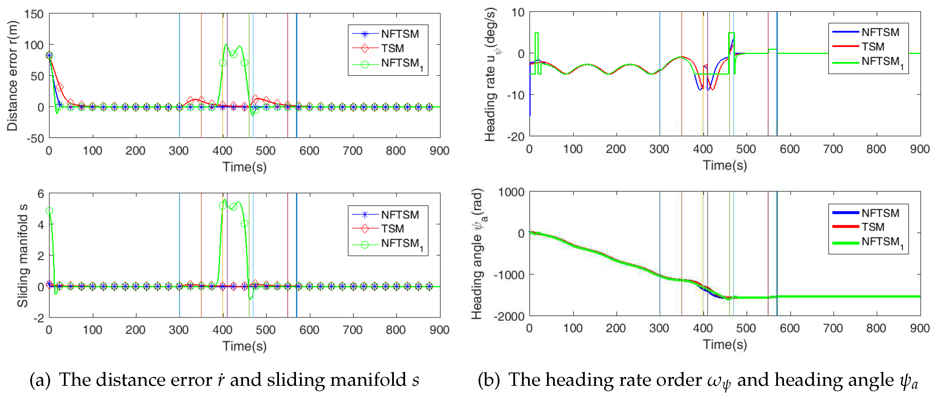
In this section, two typical maneuvering actions are designed to verify the effectiveness of the proposed algorithm for the maneuvering target: accelerated motion and sharp turn movement. Figure 9a represents the motion profile of the ground target that includes its speed and heading angle. The motion of the target is described as follows. The ground target moves from the start point m in the free environment with the initial speed m/s and the initial heading angle . Suppose that there is a homogeneous change of the speed and heading angle of the target. As shown in Figure 9a, the target accelerates from 2 m/s to 7 m/s during 300 s to 350 s and accelerates to 11 m/s during 460 s to 470 s. Meanwhile, the heading angle has three changes: , and , during 400 s to 410 s, 460 s to 470 s and 550 s to 570 s, respectively, assuming that the UAV’s initial heading angle and the simulation time is 900 s.
As shown in Figure 9b, the UAV can circle around the target which has a low speed during the start time. In addition, the UAV follows the target, which accelerates to a larger speed behind a distance during the ending time. It can be found that some adjustments are executed during the whole flight stage. The adjustments are particularly evident in the sharp turn process of the target.
From Figure 10a, with the changing of the target speed and heading angle, all three of the algorithms can make the state converge to the desired position. Before the target changes its motion state, the NFTSM algorithm can make the distance error r converge to less than 0.0001 m in 24.3 s, while takes 34.2 s with oscillatory convergence. However, the TSM algorithm converges to the desired distance error range in 113.6 s. This result confirms that the proposed algorithm can converge quickly to the desired position again.
When the target starts to accelerate movement from 300 s to 350 s, only the TSM has a large distance error of about 17.4 m, while both NFTSM and are stable. The TSM algorithm converges close to zero gradually when the speed of the target is not changing after 350 s. The larger distance error for the TSM occurs at about 460 s where the target motion has high acceleration and sharp left turn. However, the distance error for the TSM is still close to zero at 550 s where the target has a left turn again. Therefore, it proved that the TSM algorithm is sensitive to speed change of the target and insensitive to angle changing. There is an opposite phenomenon for the algorithm as shown in Figure 10a. It is easy to find that the proposed NFTSM guidance law can keep the distance error steady (only has a m error range) whether the speeding or angle changing. Hence, robustness against the target’s speed and heading angle disturbances can be demonstrated for the proposed NFTSM algorithm. It is more sensitive for angle changing than speed according to the analysis of .
The heading angle and the angle rate is given in Figure 10b. It can be found that the input limit is only executed by in order to verify the influence by the unlimited maximum command of NFTSM and TSM. This is the reason why there is too large of a change in distance error for in Figure 10a. From 350 s to 400 s, there is about a 10.3 s delay compared to NFTSM and TSM such that NFTSM can converge in a quick amount of time.
5. Conclusions
This paper focuses on the problem of moving target tracking for fixed-wing UAV in a planar environment. A modified NFTSM guidance law is proposed to solve this problem. For the sake of solving the singularity problem, which can be occurred in the traditional TSM, a modified saturation function is used through a small range around the null point. Based on Lyapunov-based approach, theoretical analysis shows that the proposed method can guarantee the reaching phase to converge in finite-time as well as the sliding phase. Compared to the traditional SMC method, the proposed guidance law can steer the UAV to reach the desired distance in a short time. Meanwhile, the body constraints can be satisfied. Adopting three kinds of the target’s motion state demonstrates that the proposed guidance law can be suitable for the problem of tracking the high maneuvering target. The proposed method is proven to converge to zero in a shorter time. The simulation results also confirm that the coefficients and can reduce the convergence time but bring the shock near the equilibrium point. In our future research, we will extend the method on the problem of multi-target tracking by multi-UAVs and will attempt to perform the NFTSM guidance law on the real UAV platform.
Acknowledgments
The authors would like to express their acknowledgement for the support from the Aviation Science Foundation of China (No. 20135851043).
Author Contributions
Kun Wu and Zhihao Cai conceived and designed the experiments; Kun Wu performed the experiments; Jiang Zhao analyzed the data; Kun Wu wrote the paper; and Zhihao Cai and Yingxun Wang provided some suggestions and revised the paper.
Conflicts of Interest
The authors declare no conflict of interest.
Abbreviations
The following abbreviations are used in this manuscript:
| UAV | Unmanned Aerial Vehicle |
| SMC | Sliding Model Control |
| NFTSM | Nonsingular Fast Terminal Sliding Mode |
| TSM | Terminal Sliding Mode |
| EKF | Extended Kalman Filter |
| , | UAV horizontal position |
| , | UAV airspeed and heading angle |
| , | UAV groundspeed and course angle |
| , , , | The motion state of target |
| L | Distance from target to UAV |
| Desired separation distance | |
| r | Distance error |
| Azimuth angle of UAV in target-frame | |
| Auxiliary parameter about azimuth angle | |
| , , | Auxiliary heading angle of UAV, target and wind |
| Steady value of UAV | |
| Heading angle error | |
| s | Sliding manifold |
| ℓ | Auxiliary parameter about distance error |
| , ,, , | NFTSM manifold parameters |
| , , | NFTSM fast reaching law parameters |
| UAV command |
References
- Rucco, A.; Aguiar, A.P.; Pereira, F.L.; de Sousa, J.B. A Predictive Path-Following Approach for Fixed-Wing Unmanned Aerial Vehicles in Presence of Wind Disturbances. In Proceedings of the Robot 2015: Second Iberian Robotics Conference, Lisbon, Portugal, 19–21 November 2015; pp. 623–634. [Google Scholar]
- Zhang, X.; Chen, J.; Xin, B.; Peng, Z. A memetic algorithm for path planning of curvature-constrained UAVs performing surveillance of multiple ground targets. Chin. J. Aeronaut. 2014, 27, 622–633. [Google Scholar] [CrossRef]
- Zhu, Q.; Zhou, R.; Zhang, J. Connectivity Maintenance Based on Multiple Relay UAVs Selection Scheme in Cooperative Surveillance. Appl. Sci. 2017, 7, 8. [Google Scholar] [CrossRef]
- Zhou, Y.; Bao, Z.; Wang, R.; Qiao, S.; Zhou, Y. Quantum Wind Driven Optimization for Unmanned Combat Air Vehicle Path Planning. Appl. Sci. 2015, 5, 1457–1483. [Google Scholar] [CrossRef]
- Sujit, P.B.; Saripalli, S.; Sousa, J.B. Unmanned Aerial Vehicle Path Following: A Survey and Analysis of Algorithms for Fixed-Wing Unmanned Aerial Vehicless. IEEE Control Syst. 2014, 34, 42–59. [Google Scholar] [CrossRef]
- Park, S. Circling over a Target with Relative Side Bearing. J. Guid. Control Dyn. 2016, 39, 1454–1458. [Google Scholar] [CrossRef]
- Lee, J.; Huang, R.; Vaughn, A.; Xiao, X.; Hedrick, J.K.; Zennaro, M.; Sengupta, R. Strategies of path-planning for a UAV to track a ground vehicle. In Proceedings of the AINS Conference, Menlo Park, CA, USA, 30 June–1 July 2003; Volume 2003. [Google Scholar]
- Shames, I.; Dasgupta, S.; Fidan, B.; Anderson, B.D.O. Circumnavigation Using Distance Measurements Under Slow Drift. IEEE Trans. Autom. Control 2012, 57, 889–903. [Google Scholar] [CrossRef]
- Oh, H.; Kim, S.; Shin, H.S.; White, B.A.; Tsourdos, A.; Rabbath, C.A. Rendezvous and standoff target tracking guidance using differential geometry. J. Intell. Robot. Syst. 2013, 69, 389–405. [Google Scholar] [CrossRef]
- Frew, E.W.; Lawrence, D.A.; Dixon, C.; Elston, J.; Pisano, W.J. Lyapunov guidance vector fields for unmanned aircraft applications. In Proceedings of the 2007 American Control Conference, New York, NY, USA, 9–13 July 2007; pp. 371–376. [Google Scholar]
- Yao, P.; Wang, H.; Su, Z. Cooperative path planning with applications to target tracking and obstacle avoidance for multi-UAVs. Aerosp. Sci. Technol. 2016, 54, 10–22. [Google Scholar] [CrossRef]
- Quigley, M.; Goodrich, M.A.; Griffiths, S.; Eldredge, A.; Beard, R.W. Target acquisition, localization, and surveillance using a fixed-wing mini-UAV and gimbaled camera. In Proceedings of the 2005 IEEE International Conference on Robotics and Automation, Barcelona, Spain, 18–22 April 2005; IEEE: Piscataway, NJ, USA, 2005; pp. 2600–2605. [Google Scholar]
- Zhang, M.; Liu, H.H. Game-theoretical persistent tracking of a moving target using a unicycle-type mobile vehicle. IEEE Trans. Ind. Electron. 2014, 61, 6222–6233. [Google Scholar] [CrossRef]
- Kim, S.; Oh, H.; Tsourdos, A. Nonlinear model predictive coordinated standoff tracking of a moving ground vehicle. J. Guid. Control Dyn. 2013, 36, 557–566. [Google Scholar] [CrossRef]
- Prevost, C.G.; Thériault, O.; Desbiens, A.; Poulin, E.; Gagnon, E. Receding horizon model-based predictive control for dynamic target tracking: A comparative study. In Proceedings of the AIAA Guidance, Navigation, and Control Conference, Chicago, IL, USA, 10–13 August 2009. [Google Scholar]
- Narkiewicz, J.P.; Kopyt, A.; Radyisyewski, P.; Malecki, T. Optimal selection of UAV for ground target tracking. In Proceedings of the AIAA Modeling and Simulation Technologies Conference, Dallas, TX, USA, 22–26 June 2015. [Google Scholar]
- Tan, C.K.; Wang, J.; Paw, Y.C.; Ng, T.Y. Tracking of a moving ground target by a quadrotor using a backstepping approach based on a full state cascaded dynamics. Appl. Soft Comput. 2016, 47, 47–62. [Google Scholar] [CrossRef]
- Zhang, M.; Liu, H.H. Cooperative Tracking a Moving Target Using Multiple Fixed-wing UAVs. J. Intell. Robot. Syst. 2016, 81, 505–529. [Google Scholar] [CrossRef]
- Oh, H.; Kim, S.; Tsourdos, A.; White, B.A. Decentralised standoff tracking of moving targets using adaptive sliding mode control for UAVs. J. Intell. Robot. Syst. 2014, 76, 169–183. [Google Scholar] [CrossRef]
- Gazi, V.; Fidan, B.; Ordóñez, R.; Köksal, M.İ. A target tracking approach for nonholonomic agents based on artificial potentials and sliding mode control. J. Dyn. Syst. Meas. Control 2012, 134, 061004. [Google Scholar] [CrossRef]
- Modirrousta, A.; Sohrab, M.; Dehghan, S.M.M. A modified guidance law for ground moving target tracking with a class of the fast adaptive second-order sliding mode. Trans. Inst. Meas. Control 2016, 38, 819–831. [Google Scholar] [CrossRef]
- Jinkun, L. Sliding Mode Control Design And MATLAB Simulation: The Basic Theory and Design Method; Tsinghua University Press: Beijing, China, 2015. [Google Scholar]
- Harl, N.; Balakrishnan, S. Impact time and angle guidance with sliding mode control. IEEE Trans. Control Syst. Technol. 2012, 20, 1436–1449. [Google Scholar] [CrossRef]
- Song, J.; Song, S.; Zhou, H. Adaptive nonsingular fast terminal sliding mode guidance law with impact angle constraints. Int. J. Control Autom. Syst. 2016, 14, 99–114. [Google Scholar] [CrossRef]
- Miao, C.X.; Fang, J.C. An adaptive three-dimensional nonlinear path following method for a fix-wing micro aerial vehicle. Int. J. Adv. Robot. Syst. 2012, 9, 206. [Google Scholar] [CrossRef]
- Liang, Y.; Jia, Y. Combined vector field approach for 2D and 3D arbitrary twice differentiable curved path following with constrained UAVs. J. Intell. Robot. Syst. 2016, 83, 133–160. [Google Scholar] [CrossRef]
- Bar-Shalom, Y.; Li, X.R.; Kirubarajan, T. Estimation with Applications to Tracking and Navigation: Theory Algorithms and Software; John Wiley & Sons: Hoboken, NJ, USA, 2001. [Google Scholar]
- Karsaz, A.; Ahari, A.A. Backward input estimation algorithm for tracking maneuvering target. In Proceedings of the 2016 24th Iranian Conference on Electrical Engineering (ICEE), Shiraz, Iran, 10–12 May 2016; IEEE: Piscataway, NJ, USA, 2016; pp. 745–750. [Google Scholar]
- Ma, L.; Hovakimyan, N. Cooperative target tracking in balanced circular formation: Multiple UAVs tracking a ground vehicle. In Proceedings of the 2013 American Control Conference, Washington, DC, USA, 17–19 June 2013; IEEE: Piscataway, NJ, USA, 2013; pp. 5386–5391. [Google Scholar]
- Yu, S.; Yu, X.; Shirinzadeh, B.; Man, Z. Continuous finite-time control for robotic manipulators with terminal sliding mode. Automatica 2005, 41, 1957–1964. [Google Scholar] [CrossRef]
- Yang, L.; Yang, J. Nonsingular fast terminal sliding-mode control for nonlinear dynamical systems. Int. J. Robust Nonlinear Control 2011, 21, 1865–1879. [Google Scholar] [CrossRef]
- Gradshteyn, I.S.; Ryzhik, I.M. Table of Integrals, Series, and Products; Academic Press: Cambridge, MA, USA, 2014. [Google Scholar]
- Khalil, H.K. Noninear Systems, 3rd ed.; Publishing House of Electronics Indystry: Beijing, China, 2012. [Google Scholar]
Figure 1.
Tracking geometry between the target and unmanned aerial vehicle (UAV).
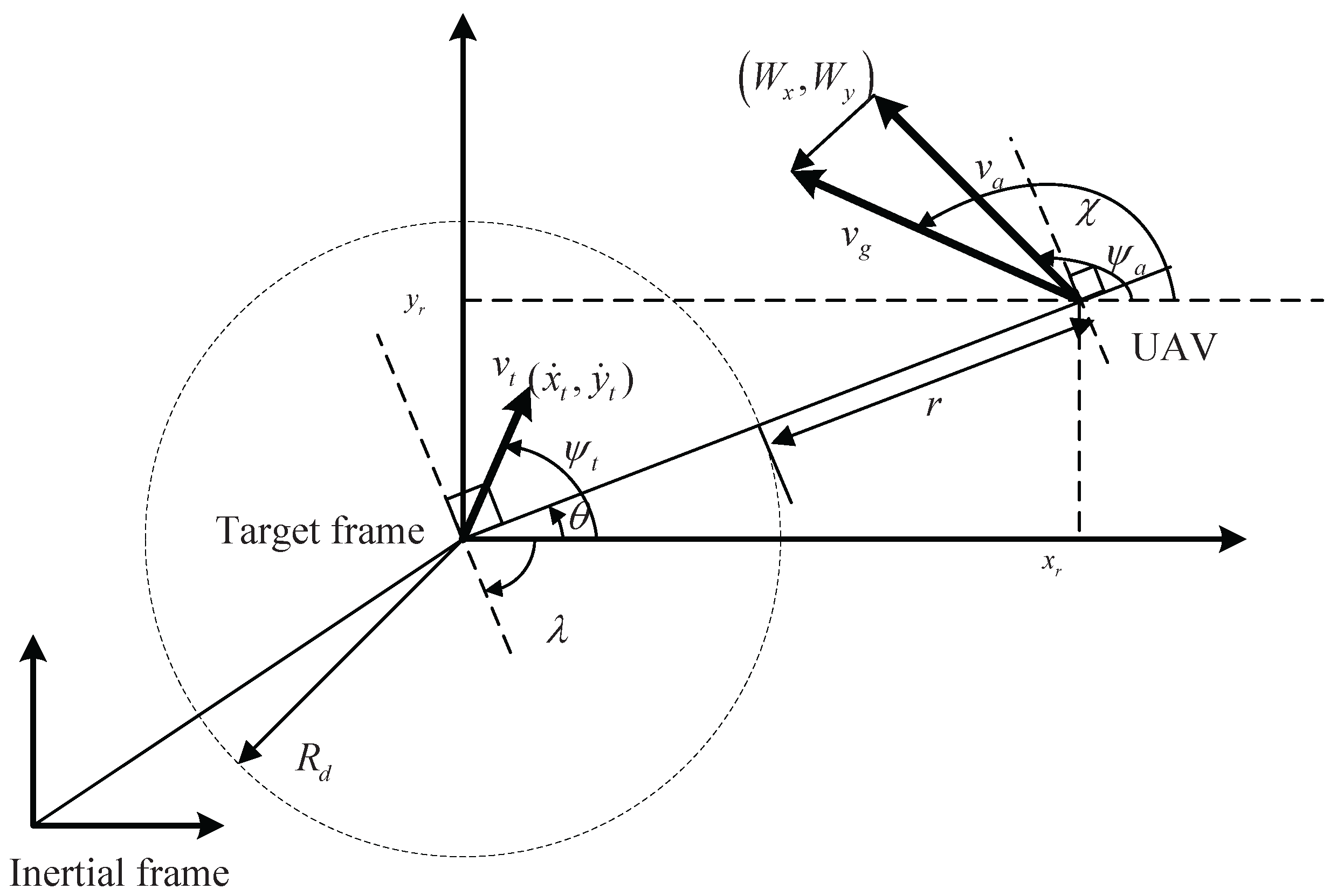
Figure 2.
The Parameter analysis of terminal sliding mode (TSM).

Figure 3.
The comparison of different fast terminal sliding modes (FTSMs).
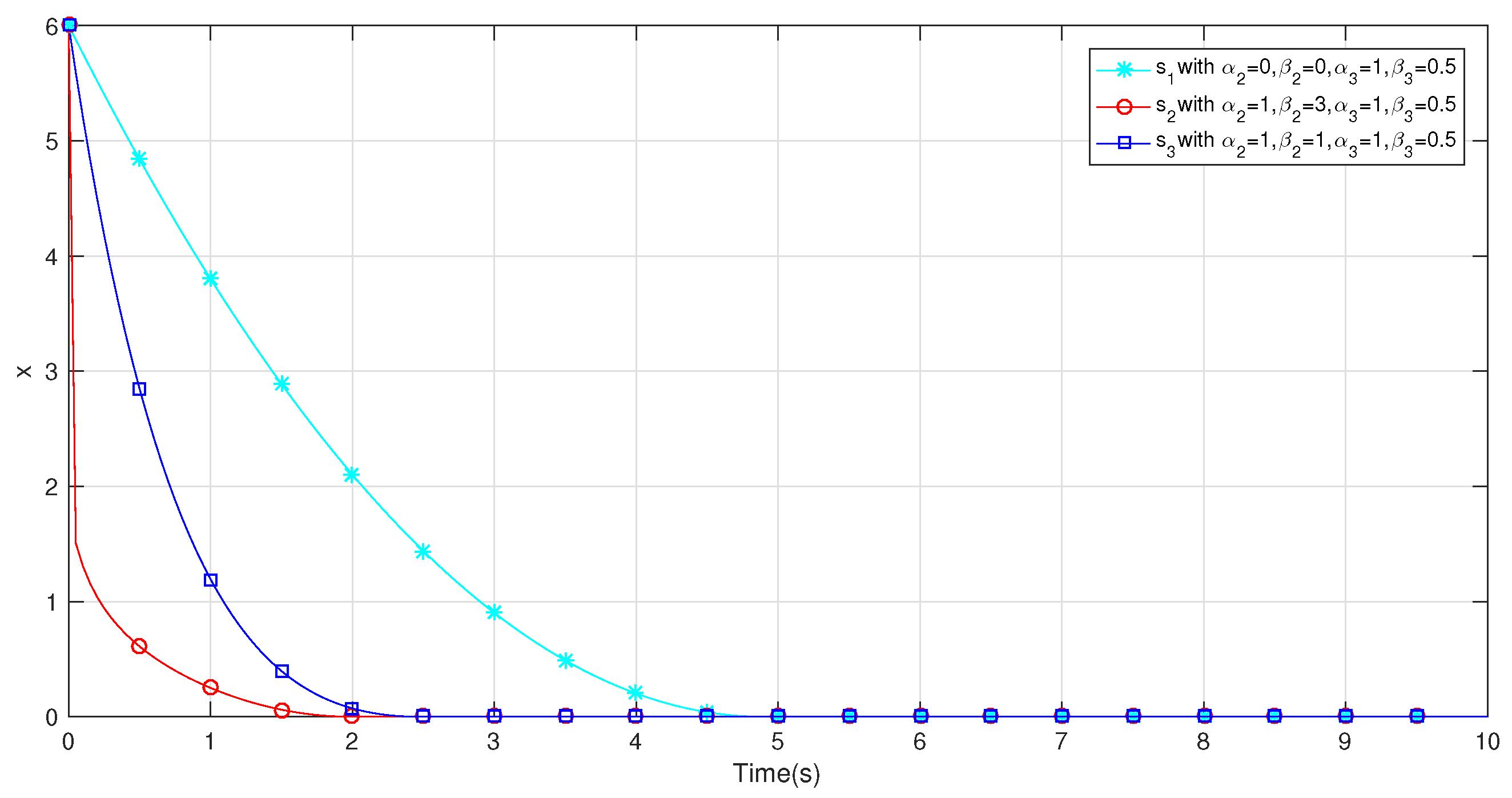
Figure 4.
Tracking a stationary target with different initial heading angles.
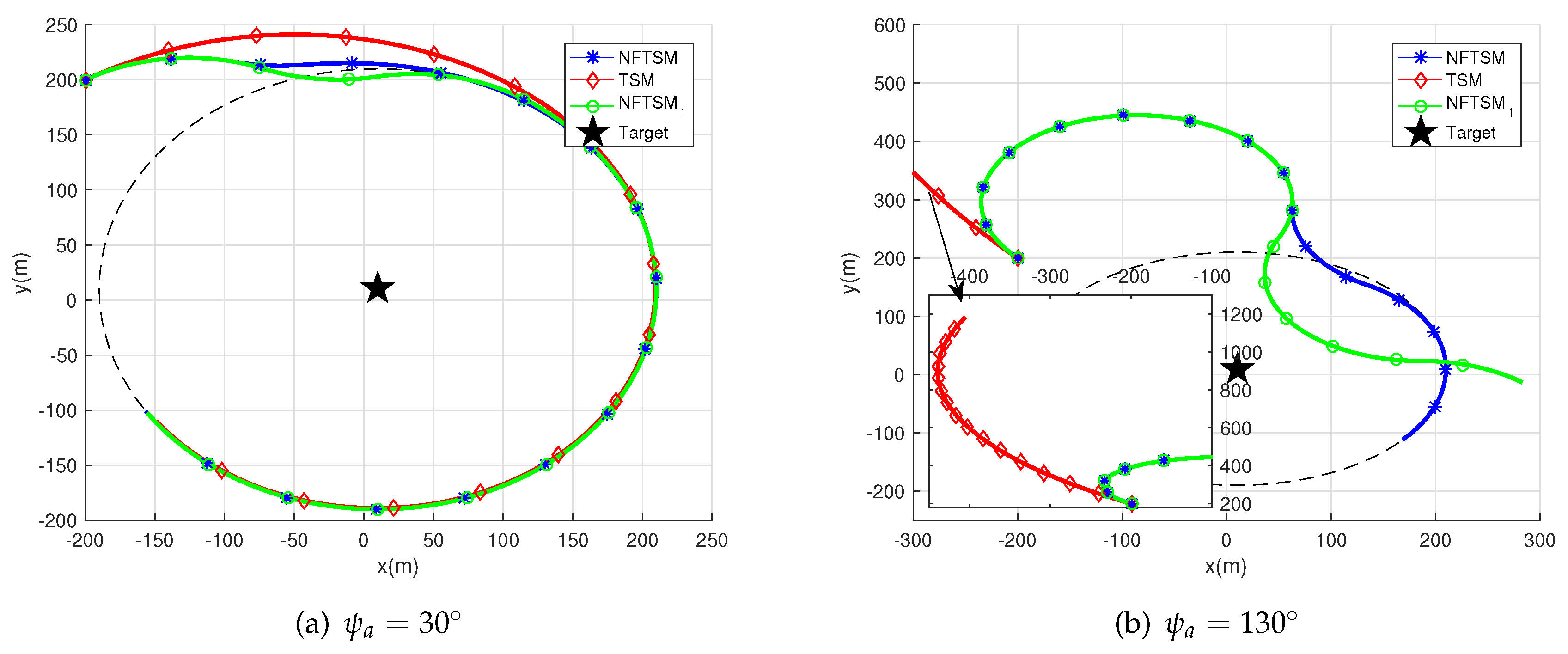
Figure 5.
The results of tracking a stationary target with .

Figure 6.
The results of tracking a stationary target with .

Figure 7.
Tracking a moving target along the S-shape trajectory.

Figure 8.
The result of tracking a moving target along the S-shape trajectory.
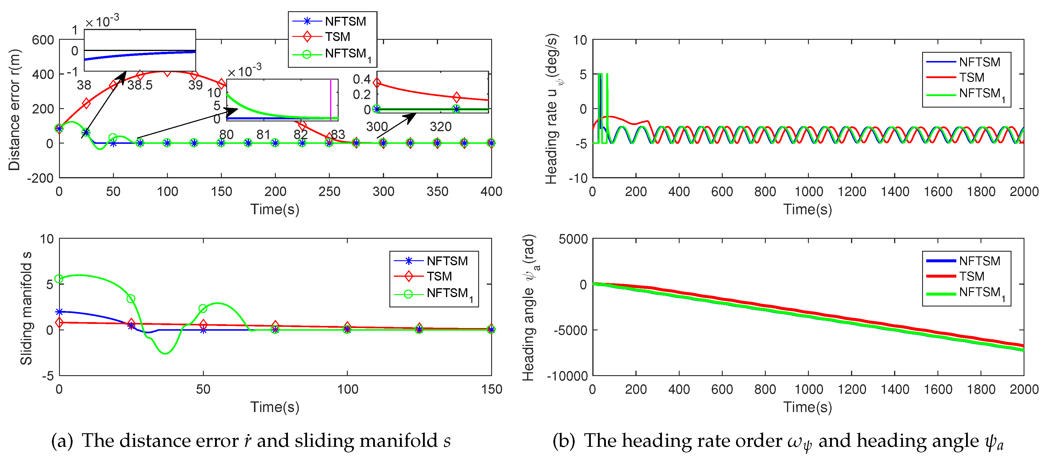
Figure 9.
The trajectory of the moving target and the UAV.
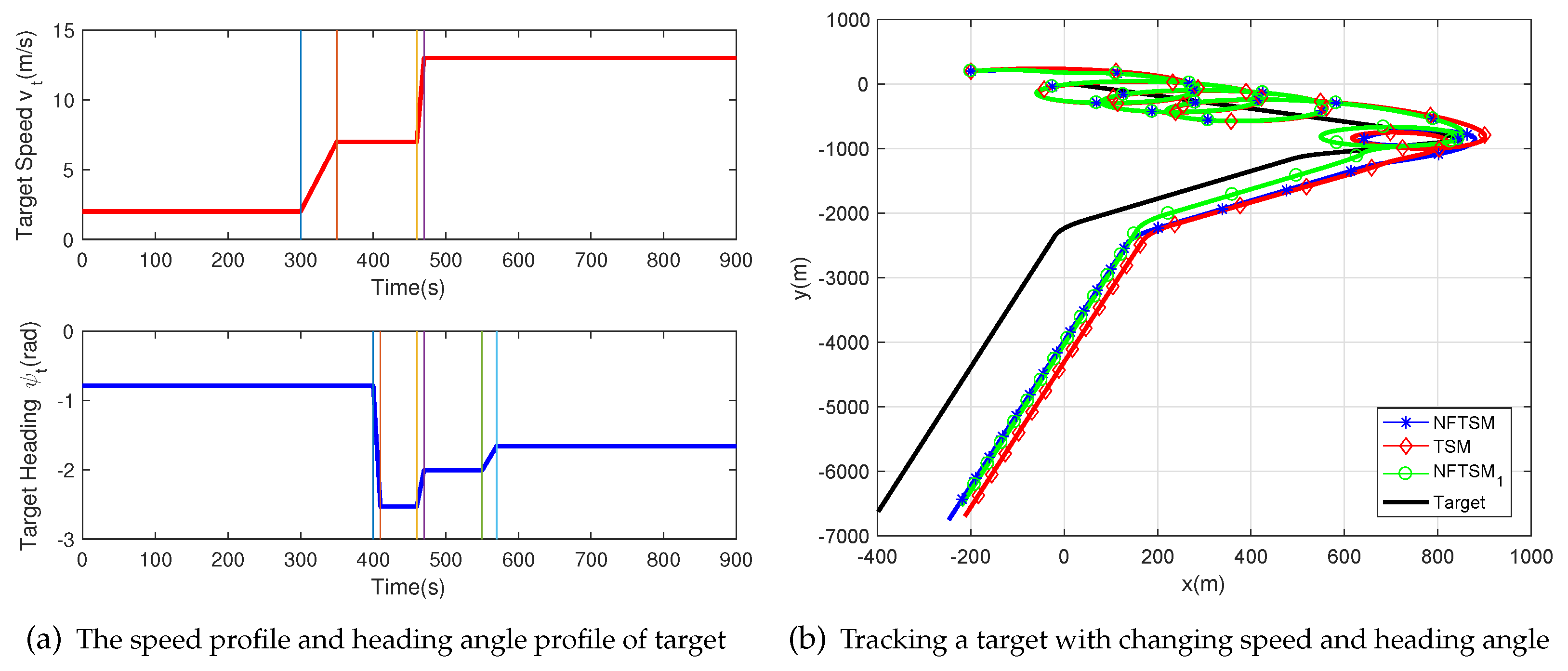
Figure 10.
The results of tracking a maneuvering target.


Table 1.
Parameters of target tracking, UAV: unmanned aerial vehicle.
| Initial Condition | Value |
|---|---|
| Sampling time, (s) | 0.5 |
| UAV initial position, (m) | [−200,200] |
| Constant airspeed, (m/s) | 13 |
| Maximum turn rate, | 5 |
| Desired distance, (m) | 200 |
| Target initial position, (m) | [10,10] |
| Target initial velocity, (m/s) | 2 |
| Wind speed, (m/s) | [0.1,0.2] |
Table 2.
Coefficients of the different guidance laws, TSM: terminal sliding mode, NFTSM: nonsingular fast TSM, : NFTSM with another set of coefficients.
Table 2.
Coefficients of the different guidance laws, TSM: terminal sliding mode, NFTSM: nonsingular fast TSM, : NFTSM with another set of coefficients.
| Algorithm | Coefficient | ||||
|---|---|---|---|---|---|
| NFTSM | , | , | , | , | |
| , | , | , | |||
| TSM | , | , | , | ||
| , | , | , | , | ||
| , | , | , | |||
Table 3.
The convergence time of stationary target tracking.
| Algorithm | Case () | Simulation Time (s) | Convergence Time (s) | Distance Error r (m) |
|---|---|---|---|---|
| NFTSM | 80 | 31.2 | less than 0.0001 | |
| TSM | 80 | 80 | −0.742 | |
| 80 | 37.3 | less than 0.0001 | ||
| NFTSM | 100 | 72.9 | less than 0.0001 | |
| TSM | 100 | 100 | no convergence | |
| 100 | 100 | shock |
© 2017 by the authors. Licensee MDPI, Basel, Switzerland. This article is an open access article distributed under the terms and conditions of the Creative Commons Attribution (CC BY) license (http://creativecommons.org/licenses/by/4.0/).
Share and Cite
MDPI and ACS Style
Wu, K.; Cai, Z.; Zhao, J.; Wang, Y. Target Tracking Based on a Nonsingular Fast Terminal Sliding Mode Guidance Law by Fixed-Wing UAV. Appl. Sci. 2017, 7, 333. https://doi.org/10.3390/app7040333
AMA Style
Wu K, Cai Z, Zhao J, Wang Y. Target Tracking Based on a Nonsingular Fast Terminal Sliding Mode Guidance Law by Fixed-Wing UAV. Applied Sciences. 2017; 7(4):333. https://doi.org/10.3390/app7040333
Chicago/Turabian StyleWu, Kun, Zhihao Cai, Jiang Zhao, and Yingxun Wang. 2017. "Target Tracking Based on a Nonsingular Fast Terminal Sliding Mode Guidance Law by Fixed-Wing UAV" Applied Sciences 7, no. 4: 333. https://doi.org/10.3390/app7040333
Note that from the first issue of 2016, this journal uses article numbers instead of page numbers. See further details here.