Pulse Propagation Models with Bands of Forbidden Frequencies or Forbidden Wavenumbers: A Consequence of Abandoning the Slowly Varying Envelope Approximation and Taking into Account Higher-Order Dispersion

Abstract

We study linear and nonlinear pulse propagation models whose linear dispersion relations present bands of forbidden frequencies or forbidden wavenumbers. These bands are due to the interplay between higher-order dispersion and one of the terms (a second-order derivative with respect to the propagation direction) which appears when we abandon the slowly varying envelope approximation. We show that as a consequence of these forbidden bands, narrow pulses radiate in a novel and peculiar way. We also show that the nonlinear equations studied in this paper have exact soliton-like solutions of different forms, some of them being embedded solitons. The solutions obtained (of the linear as well as the nonlinear equations) are interesting since several arguments suggest that the Cauchy problems for these equations are ill-posed, and therefore the specification of the initial conditions is a delicate issue. It is also shown that some of these equations are related to elliptic curves, thus suggesting that these equations might be related to other fields where these curves appear, such as the theory of modular forms and Weierstrass ℘ functions, or the design of cryptographic protocols.

1. Introduction

The nonlinear Schrödinger (NLS) equation:

$$i\frac{\partial u}{\partial z}+{\epsilon }_2\frac{{\partial }^{2}u}{\partial t^2}+{\gamma }_1{\left|u\right|}^{2}u=0$$

(1)

plays a central role in the study of light pulses propagating in optical fibers. In this equation z represents the distance along an optical fiber, t is the so-called retarded time, $u\left(z,t\right)$ is the envelope of the electric field of a laser beam, ${\epsilon }_2$ is a real constant whose value depends on the laser´s frequency, and ${\gamma }_1$ depends on the characteristics of the fiber (and also on the frequency of the light). It is worth mentioning that Equation (1) is sometimes referred to as the temporal NLS equation, to distinguish it from the spatial NLS equation, whose physical meaning is different, even though it has the same form as Equation (1), but with a spatial variable x (corresponding to a transversal coordinate) instead of the retarded time t.

In spite of its great importance, it should be remembered that Equation (1) is an approximate equation. In order to arrive at this equation several terms have been neglected. Some of these neglected terms are the following:

(a)

$-i{u}_{ttt}$ and/or $u_{4t}$: these higher-order derivatives are necessary to describe sub-picosecond pulses [1,2,3,4,5,6,7,8,9,10,11,12]; in particular, conditions for including $u_{4t}$ and discarding $-i{u}_{ttt}$ are discussed in [7,9],

(b)

${\left|u\right|}^{4}u$: this higher-order nonlinearity is used when we want to describe the propagation of pulses when the light intensity approaches the values which produce the “saturation” of the refractive index [13,14,15,16,17,18,19,20],

(c)

$i{({\left|u\right|}^{2}u)}_t$: this term is necessary to describe the self-steepening of the optical pulses [21,22,23],

(d)

$u{({\left|u\right|}^2)}_t$: this term is associated with the effect of Raman scattering [24,25,26,27].

The effects of including these terms in generalized NLS equations have been thoroughly studied in the literature. Moreover, an additional approximation introduced in the deduction of the NLS equation is the slowly-varying-envelope approximation (SVEA). This approximation is adequate when the complex amplitude of an optical pulse varies slowly in space and time. However, when we deal with optical pulses whose widths only contain a few cycles of the carrier wave, it is necessary to improve the SVEA. Several alternatives have been proposed to improve this approximation. As early as 1985, Christodoulides and Joseph studied an extended NLS equation which contained higher-order dispersion and the additional terms $u_{zz}$, $i{({\left|u\right|}^{2}u)}_{\tau }$ and ${({\left|u\right|}^{2}u)}_{\tau \tau }$, where τ was the standard (laboratory) time [28], and they found an interesting exact soliton solution by an algebraic tour de force. In more recent times completely different models have been proposed to describe ultra-short optical pulses, and the famous Kortweg-de Vries (KdV), modified KdV (mKdV) and sine-Gordon (sG) equations have been found useful for this purpose, as well as a combination of the last two of these equations [29,30]. Another two equations which have been useful to describe ultra-short spatiotemporal pulses are a two-dimensional sG equation [31] and a cubic generalized Kadomtsev-Petviashvili (cgKP) equation [32,33]. It is worth observing that in all these models (KdV, mKdV, sG, mKdV-sG, 2D-sG and cgKP) the temporal variable which appears in the equations is a delayed time (not the laboratory time), similar to the retarded time that appears in the standard NLS equation.

In the context of spatial solitons the paraxial approximation plays a role analogous to the SVEA in temporal solitons, and the effects of nonparaxiality have also been studied. In particular, the following non-paraxial extensions of the spatial NLS equation have been studied [34,35,36]:

$$i{u}_z+\alpha u_{zz}+\frac{1}{2}{u}_{xx}+{\left|u\right|}^{2}u=0$$

(2)

$$i{u}_z+\alpha u_{zz}+{\epsilon }_2{u}_{xx}-{\gamma }_1{\left|u\right|}^{2}u+{\gamma }_2{\left|u\right|}^{4}u=0$$

(3)

The study of Equation (2) addresses a basic question which might be of interest to any reader interested in optical solitons: what is the effect of introducing the non-paraxial term $u_{zz}$ in the standard NLS equation? On the other hand, the study of Equation (3) considers an equally interesting question, albeit a slightly more specialized one: what is the effect of taking into account simultaneously nonparaxiality and higher-order nonlinearities? This question suggests that in the field of temporal solitons it would be interesting to investigate the effect of taking into account simultaneously non-SVEA terms, higher-order dispersion and higher-order nonlinearities such as ${\left|u\right|}^{4}u$. A study of this type was carried out in Ref. [28], where a model with these characteristics was proposed (except that the nonlinearity ${\left|u\right|}^{4}u$ was not considered). Complex models of this type, which include many different terms, may provide adequate descriptions for the behavior of very short pulses. However, in such models it might be difficult to appreciate the individual effect of each of the terms which have been taken into account.

In the present communication we are interested in studying approximate linear and nonlinear pulse propagation models which incorporate higher-order dispersion, higher-order nonlinearities and one of the terms that appear when we drop the SVEA (a second-order derivative with respect to the propagation direction). When we abandon the SVEA, the terms $u_{zz}$, $i{({\left|u\right|}^{2}u)}_{\tau }$ and ${({\left|u\right|}^{2}u)}_{\tau \tau }$ must be introduced in the NLS equation (τ being the standard laboratory time). However, if we use the retarded time to describe the propagation of the optical pulses, in addition to the term $u_{zz}$, it is also necessary to introduce a mixed derivative of the form $u_{zt}$ in the resulting equation [37]. To study the complete equation containing these two derivatives ($u_{zz}$ and $u_{zt}$), the nonlinear terms $i{({\left|u\right|}^{2}u)}_t$ and ${({\left|u\right|}^{2}u)}_{tt}$, an additional nonlinearity of the form ${\left|u\right|}^{4}u$, and higher-order dispersive terms ($-i{u}_{ttt}$ and/or $u_{4t}$) might be interesting and important, but it is not the objective of the present work. In this communication we are only interested in studying simplified models where the terms $u_{zt}$, $i{({\left|u\right|}^{2}u)}_t$ and ${({\left|u\right|}^{2}u)}_{tt}$ have been discarded. It is clear that these models do not pretend to provide a quantitative accurate description of a particular real system, but we will see that the study of these simplified models reveals that the simultaneous presence of the non-SVEA term $u_{zz}$ and higher-order dispersive terms such as $-i{u}_{ttt}$ or $u_{4t}$ may produce interesting results. In particular, we will show that the combined effects of these terms generate bands of forbidden frequencies, which may be related to the gaps which have been experimentally observed in the spectral profiles of very narrow pulses propagating in photonic crystal fibers [38]. Moreover, we will see that just the mathematical structure of the equations considered in this paper is interesting by itself, since we will show that these equations are related to elliptic curves, thus suggesting that a relationship may exist between the study of optical solitons and other fields where these curves play an important role, such as the abstruse theory of modular forms and Weierstrass ℘ functions, or the design of cryptographic protocols.

We will begin this communication by studying the linear equations:

$$i{u}_z+c_0{u}_{zz}+c_2{u}_{tt}-i{c}_3{u}_{ttt}=0$$

(4)

$$i{u}_z+c_0{u}_{zz}+c_2{u}_{tt}+c_4{u}_{4t}=0$$

(5)

and afterwards we will focus our attention on the nonlinear equations:

$$i{u}_z+c_0{u}_{zz}+c_2{u}_{tt}+c_4{u}_{4t}+{\gamma }_1{\left|u\right|}^{2}u-{\gamma }_2{\left|u\right|}^{4}u=0$$

(6)

$$i{u}_z+c_0{u}_{zz}+c_2{u}_{tt}-i{c}_3{u}_{ttt}+c_4{u}_{4t}+{\gamma }_1{\left|u\right|}^{2}u-{\gamma }_2{\left|u\right|}^{4}u=0$$

(7)

$$i{u}_z+c_0{u}_{zz}+c_2{u}_{tt}+c_4{u}_{4t}+{\gamma }_1{\left|u\right|}^{2}u=0$$

(8)

The study of the linear Equations (4) and (5) will reveal how the interplay between the non-SVE term $u_{zz}$ and the higher-order dispersive terms generates bands of forbidden frequencies or forbidden wavenumbers. Then, we will show that the nonlinear Equations (6)–(8) have exact solitons of different types, some of them being embedded solitons.

The structure of this paper is the following. In Section 2 we will show that the linear dispersion relations of Equations (4) and (5) have highly unusual forms. We shall see that the dispersion relation of Equation (4) is an elliptic curve, while that of Equation (5) presents bands of forbidden frequencies, or forbidden wavenumbers. As the occurrence of elliptic curves in this context opens the possibility of relating Equation (4)—or its solutions—to other areas where elliptic curves play an important role, in Appendix A we describe in more detail the basic characteristics of these curves, and in Appendix B we briefly discuss the relationship of these curves with modular forms and Fermat´s last theorem. In Section 3 we study the linear Equations (4) and (5). We will begin this section by paying attention to the fact that several results indicate that the Cauchy problems for these equations are ill-posed, and consequently the specification of initial conditions is a delicate issue. Then we present different solutions of these equations. These solutions will show that narrow pulses that evolve according to Equations (4) and (5) emit radiation in a completely novel and unexpected way, never observed in other models of optical pulses. In Section 4 exact soliton solutions of Equations (6)–(8) are presented. It is shown that Equation (6) has two different types of solitons (embedded solitons and solitons with a nonlinear frequency shift), Equation (7) has moving solitons of different heights and different velocities, and the solitons of Equation (8) are given by squared hyperbolic secants, thus proving that the interplay between the non-SVEA term $u_{zz}$ and higher-order dispersive and nonlinear terms permits the existence of different types of solitons. Finally Section 5 contains the conclusions of the paper.

2. Dispersion Relations and Elliptic Curves

2.1. Dispersion Relation of Equation (4)

Let us begin by paying attention to the form of the dispersion relation of Equation (4). If we substitute the tentative solution:

$$u\left(z,t\right)=\epsilon exp\left(i\left(kz-\omega t\right)\right)$$

(9)

in Equation (4), the following dispersion relation is easily found:

$$c_0{k}^2+k=c_3{\omega }^3-c_2{\omega }^2$$

(10)

and this equation can be rescaled by defining $\tilde{k}=c_0^{1/2}k$ and $\tilde{\omega }=c_3^{1/3}\omega$, thus obtaining (after supressing the tildes):

$$k^2+a_{3}k={\omega }^3+a_2{\omega }^2$$

(11)

where $a_3=c_0^{-1/2}$ and $a_2=-c_2{c}_3^{-2/3}$. This equation describes an elliptic curve (if $a_2\ne 0$ and $a_3\ne 0$), which is an interesting result since elliptic curves have important roles in areas which might seem completely unrelated to the study of light pulses in optical fibers, such as the abstruse theory of modular forms [39], or the development of cryptographic protocols [40]. For the sake of simplicity in the following we will also say that Equation (10) itself is an elliptic curve, although, being rigorous, we should say that Equation (10) is an elliptic curve up to scaling. In other words, it is an elliptic curve distorted by a non-uniform scaling (i.e., a scale transformation which applies different scale factors in the k and ω axes).

Now let us pay more attention to the shape of the curves described by the dispersion relation (10). From Equation (10) it follows that the wavenumber k is given by the following function of the frequency:

$$k\left(\omega \right)=\frac{-1\pm \sqrt{1-4c_0\left(c_2{\omega }^2-c_3{\omega }^3\right)}}{2c_0}$$

(12)

and the form of this function is quite different from the dispersion relations found in other optical systems. If we choose, for example, the coefficients $c_0=1/30$, $c_2=1/2$ and $c_3=1/15$, the form of the curve $k\left(\omega \right)$ is shown in Figure 1.

We can see that the curve is symmetrical with respect to a horizontal line, but completely asymmetrical with respect to the k-axis, which is an unusual behavior. However, the behavior of $k\left(\omega \right)$ can be more bizarre. If we choose the coefficients $c_0=1/40$, $c_2=1/2$ and $c_3=1/50$, $k\left(\omega \right)$ has the form shown in Figure 2.

We can see that in this case the dispersion relation exhibits two bands of forbidden frequencies, thus implying that small-amplitude linear waves cannot propagate with frequencies in the ranges:

$$-\infty <\omega <{\omega }_1 \mathrm{and} {\omega }_2<\omega <{\omega }_3,$$

(13)

where:

$${\omega }_1=10\left(1-\sqrt{2}\right), {\omega }_2=5 \mathrm{and} {\omega }_3=10\left(1+\sqrt{2}\right)$$

(14)

are the frequencies which make the radicand that appears in Equation (12) equal to zero. This radicand becomes negative for frequencies in the intervals shown in (13), and therefore $k\left(\omega \right)$ becomes complex for these frequencies. In the next section we will investigate the consequences of the existence of these bands of forbidden frequencies.

The fact that the linear dispersion relation of Equation (4) is an elliptic curve suggests that this equation might be related to other subjects where these curves also appear. In particular, a relationship may exist between optical solitons and the theory of modular forms, which played a central role in the proof of Fermat’s last theorem. For this reason in Appendix A we explain more precisely what an elliptic curve is, and in Appendix B we briefly review what was the role played by elliptic curves and modular forms in the proof of Fermat’s last theorem.

To close this sub-section it is worth observing that if we introduced the mixed derivative $u_{zt}$ in Equation (4), the resulting dispersion relation would still be an elliptic curve.

2.2. Dispersion Relation of Equation (5)

Now let us direct our attention to Equation (5). If we substitute the plane wave (9) into Equation (5) we arrive at the following dispersion relation:

$$c_0{k}^2+k+\left(c_2{\omega }^2-c_4{\omega }^4\right)=0$$

(15)

Let us now study the form of this dispersion relation in more detail. To determine the range of wavenumbers permitted by this relation it is convenient to write it in the form:

$${\omega }^2={\left(2c_4\right)}^{-1}\left\{c_2\pm \sqrt{c_2^2+4c_4\left(c_0{k}^2+k\right)}\right\}$$

(16)

This equation implies that every real value of k will be permitted (i.e., every real value of k corresponds to a positive ${\omega }^2$) if and only if:

$$c_0{c}_2^2>c_4$$

(17)

In the opposite case, when:

$$c_0{c}_2^2<c_4$$

(18)

the dispersion relation contains a band of forbidden wavenumbers. When the condition (18) is satisfied, the analysis of the function defined by Equation (16) shows that ${\omega }^2$ turns out to be negative if k is in the interval:

$$k_1<k<k_2$$

(19)

where:

$$k_{1,2}={\left(2c_0\right)}^{-1}\left\{-1\pm \sqrt{1-c_0{c}_2^2/c_4}\right\}$$

(20)

Therefore, when the condition (18) holds, the inequalities (19) define a band of forbidden wavenumbers.

In Figure 3 we can see the shape of the dispersion relation $k\left(\omega \right)$ defined by Equation (15) when $c_0=1/30$, $c_2=1/2$ and $c_4=1/80$. As these values satisfy the condition (18), the gap of forbidden wavenumbers seen in the figure is explained. The dashed horizontal lines indicate the wavenumbers $C_1$ and $C_2$ of the soliton solutions of Equation (6) (with ${\gamma }_1=5$ and ${\gamma }_2=1$) that will be determined in Section 4.

Now let us study in more detail what happens when the condition (17) holds. In this case the linear dispersion relation presents two bands of forbidden frequencies, which is a novel situation in the study of optical solitons. To convince ourselves that such forbidden frequency gaps really exist, it is convenient to write the linear dispersion relation (15) in the form:

$$k={\left(2c_0\right)}^{-1}\left\{-1\pm \sqrt{1-4c_0\left(c_2{\omega }^2-c_4{\omega }^4\right)}\right\}$$

(21)

This equation implies that if $c_0{c}_2^2>c_4$ holds, there are frequencies for which k turns out to be complex. Analyzing the radicand which appears on the right-hand-side of Equation (21) we find that these forbidden frequencies are in the intervals:

$$-{\omega }_2<\omega <-{\omega }_1 \mathrm{and} {\omega }_1<\omega <{\omega }_2$$

(22)

and the frequencies ${\omega }_1$ and ${\omega }_2$ are defined by:

$${\omega }_{1,2}^2={\left(2c_4\right)}^{-1}\left\{c_2\pm \sqrt{c_2^2-c_4/c_0}\right\}$$

(23)

where the minus sign corresponds to ${\omega }_1$, and the plus sign defines ${\omega }_2$. In Figure 4 we can see the shape of the dispersion relation (21) in the particular case when $c_0=1/15$, $c_2=1/2$ and $c_4=1/256$. These coefficients satisfy the condition (17), and therefore there are two bands of forbidden frequencies, as we can see in the figure. The consequences of the presence of these forbidden frequency gaps will be investigated in the following section. The dashed horizontal lines shown in this figure indicate the values of the wavenumbers of the soliton solutions of Equation (6) (with ${\gamma }_1=5$ and ${\gamma }_2=1$) that will be found in Section 4.

We now know that the dispersion relation (15) has interesting forms: when $c_0{c}_2^2<c_4$ there is a band of forbidden wavenumbers (as in Figure 3), and when $c_0{c}_2^2>c_4$ there are two bands of forbidden frequencies (as in Figure 4). The only case that we have not examined is when the coefficients $c_0$, $c_2$ and $c_4$ are on the surface defined by the equation:

$$c_0{c}_2^2=c_4$$

(24)

Only in this case (intermediate between the inequalities (17) and (18)) does the dispersion relation (15) have no gaps. An example of this case is obtained when $c_0=1/20$, $c_2=1/2$ and $c_4=1/80$. With these coefficients the shape of the dispersion relation is shown in Figure 5.

We have thus seen that the dispersion relations of Equations (4) and (5) have interesting and unusual forms. Now we will investigate the behavior of solitary waves that obey these equations.

3. The Linear Equations (4) and (5)

3.1. The Issue of the Initial Conditions

In the study of optical solitons many variants of the nonlinear Shrödinger (NLS) equation have been considered in the past in order to describe the propagation of light pulses in optical fibers under different conditions. However, different as they are, most of these variants share a common denominator: they are first-order equations with respect to the evolution variable z. This characteristic implies that in all these cases the initial condition $u\left(z=0, t\right)$ is sufficient to determine particular solutions of the corresponding equations. This fact seems to be consistent with physical reality: if we have an optical fiber (with well-defined characteristics: shape, composition, refraction index, type of cladding, etc.), and a laser beam (of known frequency) is sent into the fiber, the light intensity (as a function of time) at the beginning of the fiber (i.e., at $z=0$) is all we need to determine completely the behavior of light along the fiber.

On the other hand, the situation with Equations (4)–(8) is completely different. These equations are of second order in z, and this characteristic has two important consequences:

CONSEQUENCE 1:

With these equations we require two initial conditions, $u\left(z=0, t\right)$ and $u_z\left(z=0, t\right)$, in order to determine a particular solution. This requirement is somewhat perplexing since physical intuition suggests that $u\left(z=0, t\right)$ should be enough to determine the evolution of light along the fiber. Therefore, it seems as if we were in the presence of a contradiction: while mathematics indicates that Equations (4)–(8) require two initial conditions to define a particular solution, physics suggests that the knowledge of $u\left(0, t\right)$ should be enough to define completely the behavior of the system.

CONSEQUENCE 2:

Although formal proofs are still lacking, several arguments suggest that the Cauchy problems for Equations (4)–(8) might be ill-posed (in certain regions of the space of coefficients $c_n$). The following results permit us to understand why this ill-posedness is to be expected:

(i)

The presence of the non-paraxial term $u_{zz}$ in the equation:

$$i{u}_z+\epsilon u_{zz}+\frac{1}{2}\left(u_{xx}+u_{yy}\right)+{\left|u\right|}^{2}u=0$$

(25)

makes the Cauchy problem for this equation ill-posed [21,41].

(ii)

The presence of higher-order nonlinearities in equations of the form:

$$i{u}_z+u_{tt}+\lambda {\left|u\right|}^{m}u=0$$

(26)

makes their Cauchy problems ill-posed if $m\ge 4$ and $\lambda >0$ [42].

(iii)

The presence of higher-order derivative $u_{4t}$ in the equation:

$$u_{zz}=u_{tt}+2u_t^2+2u{u}_{tt}+u_{4t}$$

(27)

makes the Cauchy problem for this equation linearly ill-posed [43].

(iv)

The solutions of the linear Equations (4) and (5) and the linear parts of Equations (6)–(8) contain decaying as well as growing modes of the form $\exp \left(\pm \sigma z-i\omega t\right)$, as we shall see in Section 3.2 and Section 3.3. The existence of these modes makes the corresponding Cauchy problems linearly ill-posed [43].

(v)

Attemps of solving initial value problems for Equations (4)–(8) by finite differences in t, and Runge-Kutta algorithms in z, encounter difficulties that are typical of ill-posed problems.

At first sight these two consequences seem to be unrelated. However, as we explain in the following, there is a connection between them. Let us begin by paying attention to Consequence 2. If the Cauchy problems associated to Equations (4)–(8) are indeed ill-posed, then (as Hadamard first observed [44]) it would be necessary to impose certain compatibility conditions among the initial conditions, for these problems to have global solutions (i.e., solutions defined for all t). Consequently, these compatibility conditions will establish a link between the two initial conditions $u\left(z=0, t\right)$ and $u_z\left(z=0, t\right)$, thus implying that, essentially, the initial condition $u\left(z=0, t\right)$ does indeed determine the future of the system, as physical intuition suggested. In this form, the compatibility conditions required by the ill-posedness of these problems (i.e., by Consequence 2), solve the apparent contradiction contained in Consequence 1 (i.e., the contrast between the mathematical requirement of two initial conditions, and the physical suggestion that only one condition should be necessary).

In the following two sub-sections we will examine different solutions of Equations (4) and (5), corresponding to different initial conditions $u\left(z=0, t\right)$. We will see that the behavior of these solutions is particularly interesting if the initial condition is a narrow solitary wave.

3.2. Solutions of Equation (4)

Let us obtain the solution of Equation (4) corresponding to a given initial condition $u\left(0,t\right)$. We will see that we do not have to specify the value of $u_z\left(0,t\right)$.

Let us begin by calculating the Fourier transform (FT) of Equation (4) (with respect to t):

$$i{U}_z+c_0{U}_{zz}-c_2{\omega }^{2}U+c_3{\omega }^{3}U=0$$

(28)

In this equation we have defined:

$$U\left(z,\omega \right)={{\displaystyle \int }}_{-\infty }^{+\infty }u\left(z,t\right) e^{i\omega t} dt$$

(29)

The solution of Equation (28) can be obtained immediately:

$$U\left(z,\omega \right)=a\left(\omega \right) exp\left({\lambda }_{a}z\right)+b\left(\omega \right) exp\left({\lambda }_{b}z\right)$$

(30)

where ${\lambda }_a$ and ${\lambda }_b$ are the following functions of $\omega$:

$${\lambda }_{a,b}=\frac{-i\pm \sqrt{S\left(\omega \right)}}{2c_0}$$

(31)

where the plus sign in front of the radical corresponds to ${\lambda }_a$, the minus sign corresponds to ${\lambda }_b$, and the radicand $S\left(\omega \right)$ is given by:

$$S\left(\omega \right)=-1-4c_0\left(c_3{\omega }^3-c_2{\omega }^2\right)$$

(32)

From Equation (30) it follows that:

$$U_z\left(z,\omega \right)={\lambda }_{a}a\left(\omega \right) exp\left({\lambda }_{a}z\right)+{\lambda }_{b}b\left(\omega \right) exp\left({\lambda }_{b}z\right)$$

(33)

and from Equations (30) and (33) we can obtain the system:

$$U\left(0,\omega \right)=a\left(\omega \right) +b\left(\omega \right)$$

(34)

$$U_z\left(0,\omega \right)={\lambda }_{a}a\left(\omega \right)+{\lambda }_{b}b\left(\omega \right)$$

(35)

and this system gives us the values of the coefficients $a\left(\omega \right)$ and $b\left(\omega \right)$ in terms of the functions $U\left(0,\omega \right)$ and $U_z\left(0,\omega \right)$:

$$a\left(\omega \right)=\frac{U_z\left(0,\omega \right)-{\lambda }_{b}U\left(0,\omega \right)}{{\lambda }_a-{\lambda }_b}$$

(36)

$$b\left(\omega \right)=U\left(0,\omega \right)-a\left(\omega \right)$$

(37)

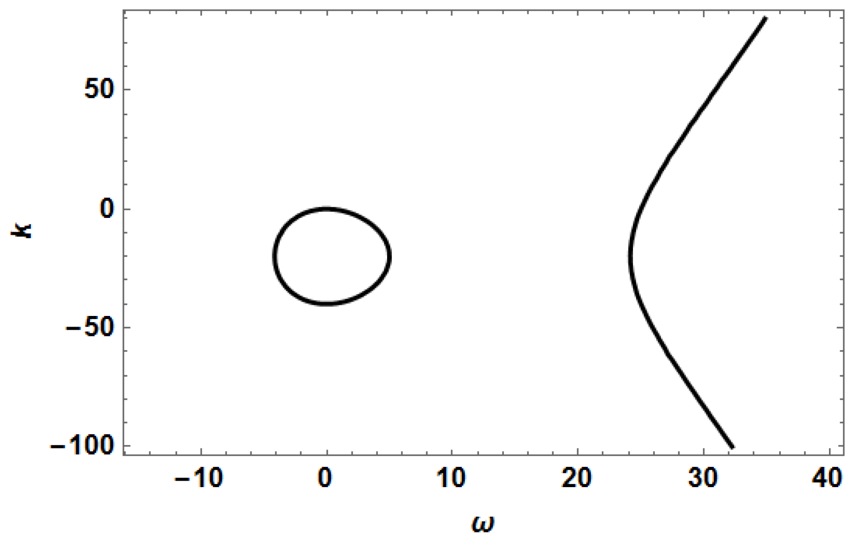
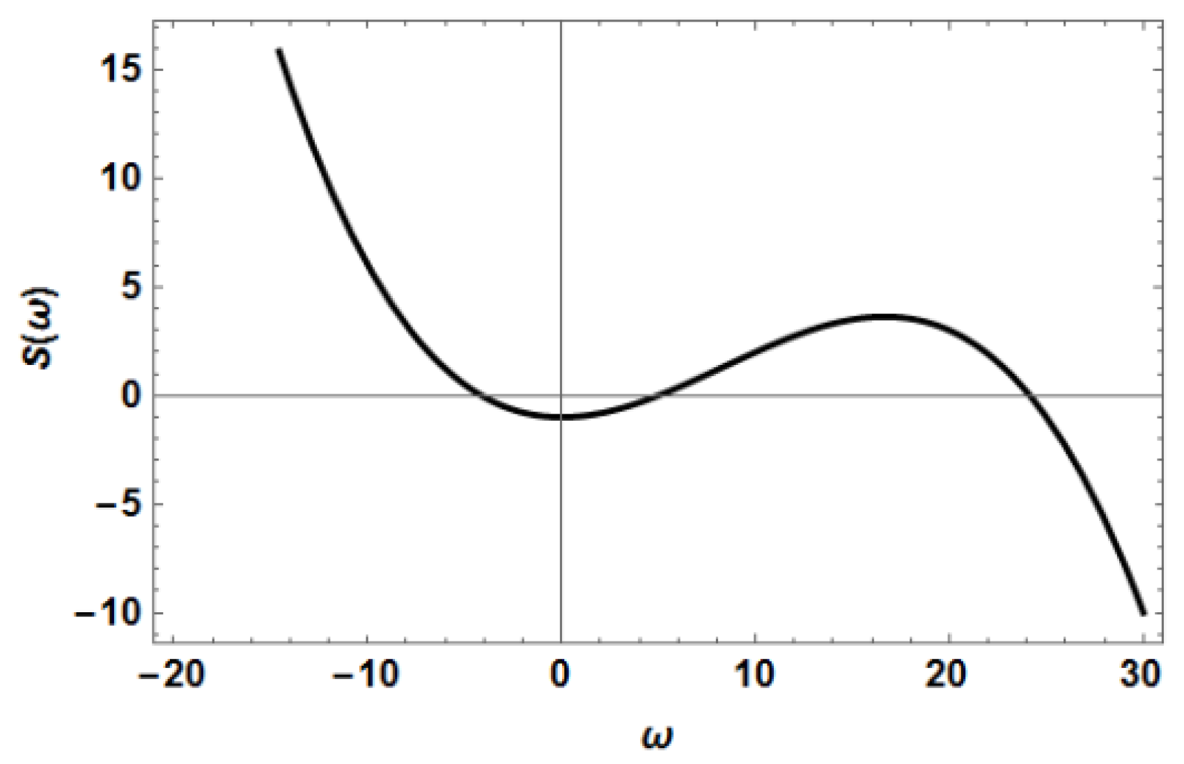
Now we can observe something interesting. Let us consider, for example, the particular case when $c_0=1/40$, $c_2=1/2$ and $c_3=1/50$. In this case the radicand $S\left(\omega \right)$ (given in (32)) has the form shown in Figure 6.

We can see in this figure that $S\left(\omega \right)>0$ if $\omega <{\omega }_1$ or ${\omega }_2<\omega <{\omega }_3$, and $S\left(\omega \right)<0$ if ${\omega }_1<\omega <{\omega }_2$ or $\omega >{\omega }_3$, where the frequencies ${\omega }_n$ are the values shown in (14). Taking into account the signs of $S\left(\omega \right)$, we can write ${\lambda }_a$ and ${\lambda }_b$ in the following way:

$${\lambda }_a=\{\begin{array}{cc}\left[-i+\sqrt{S\left(\omega \right)}\right]/2c_0,\hfill & \hfill \omega <{\omega }_1\\ \left[-i+i\sqrt{-S\left(\omega \right)}\right]/2c_0,\hfill & \hfill {\omega }_1<\omega <{\omega }_2\\ \left[-i+\sqrt{S\left(\omega \right)}\right]/2c_0,\hfill & \hfill {\omega }_2<\omega <{\omega }_3\\ \left[-i+i\sqrt{-S\left(\omega \right)}\right]/2c_0 ,\hfill & \hfill \omega >{\omega }_3\end{array}$$

(38)

$${\lambda }_b=\{\begin{array}{cc}\left[-i-\sqrt{S\left(\omega \right)}\right]/2c_0,\hfill & \hfill \omega <{\omega }_1\\ \left[-i-i\sqrt{-S\left(\omega \right)}\right]/2c_0,\hfill & \hfill {\omega }_1<\omega <{\omega }_2\\ \left[-i-\sqrt{S\left(\omega \right)}\right]/2c_0,\hfill & \hfill {\omega }_2<\omega <{\omega }_3\\ \left[-i-i\sqrt{-S\left(\omega \right)}\right]/2c_0,\hfill & \hfill \omega >{\omega }_3\end{array}$$

(39)

We can see that ${\lambda }_a$ has a positive real part when $\omega <{\omega }_1$ and ${\omega }_2<\omega <{\omega }_3$, and therefore for frequencies within these two intervals the first term on the right-hand-side (rhs) of Equation (30) grows exponentially in z. As this growth is completely unphysical (as it would imply a fictitious energy growth), the coefficient $a\left(\omega \right)$ has to be equal to zero, and consequently from Equation (36) it follows that there is an unexpected relationship between $U_z\left(0,\omega \right)$ and $U\left(0,\omega \right)$:

$$U_z\left(0,\omega \right)={\lambda }_b\left(\omega \right)U\left(0,\omega \right)$$

(40)

thus implying that:

$$u_z\left(0,t\right)=\frac{1}{2\pi }{{\displaystyle \iint }}_{-\infty }^{+\infty }{\lambda }_b\left(\omega \right) u\left(0,\tau \right) e^{i\omega \left(\tau -t\right)}d\tau d\omega$$

(41)

Therefore, as far as Equation (4) is concerned, the perplexing situation associated to the Consequence 1 (mentioned in the previous sub-section) is completely clarified: physically realistic solutions of Equation (4) are indeed completely determined by the initial condition $u\left(0,t\right)$, as physics suggested. Once $u\left(0,t\right)$ is chosen, the function $u_z\left(0, t\right)$ is determined by Equation (41).

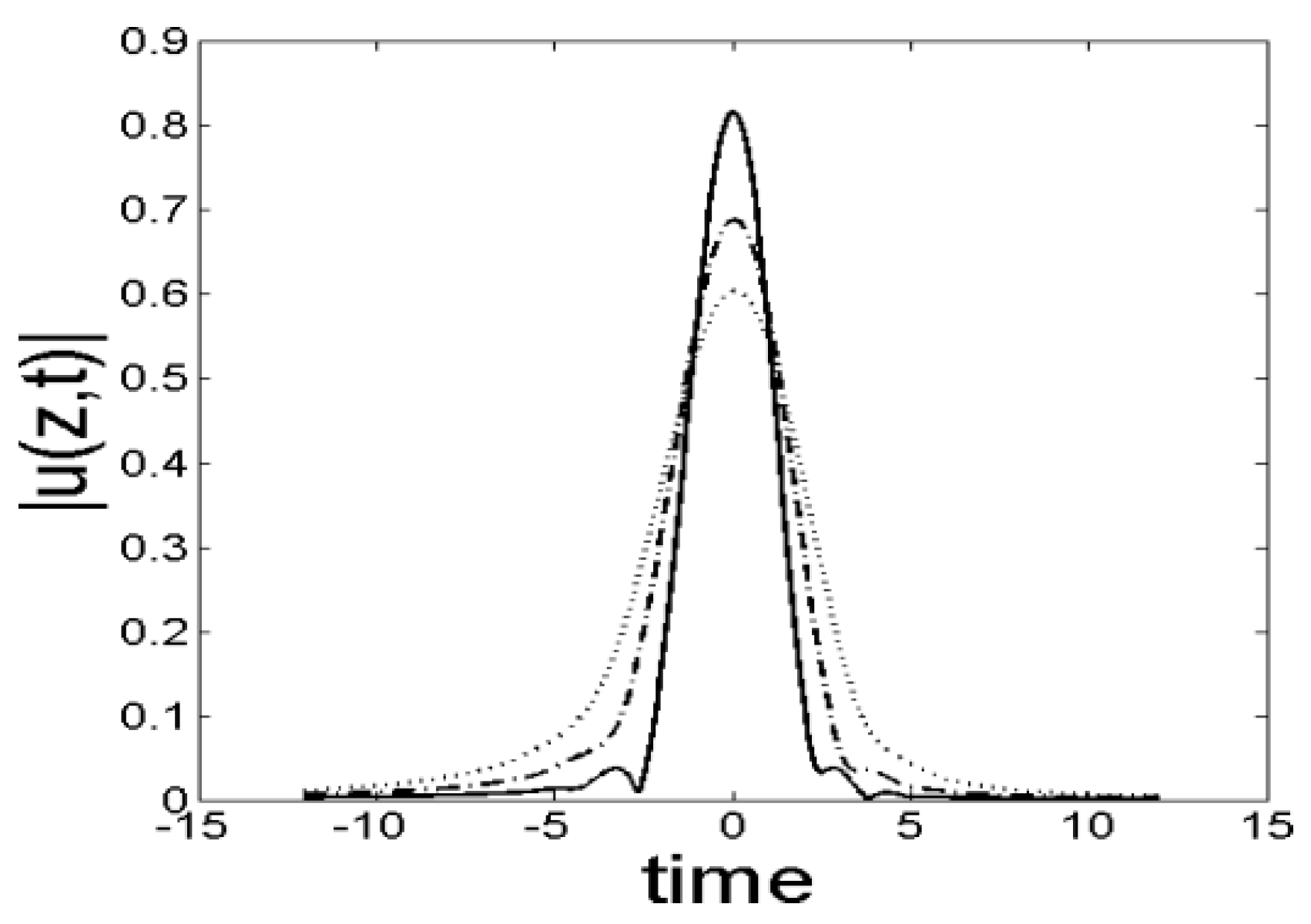
Now let us calculate the solution of Equation (4) corresponding to a soliton-like initial condition of the form:

$$u\left(0,t\right)=A \mathrm{sech}\left(Bt\right)$$

(42)

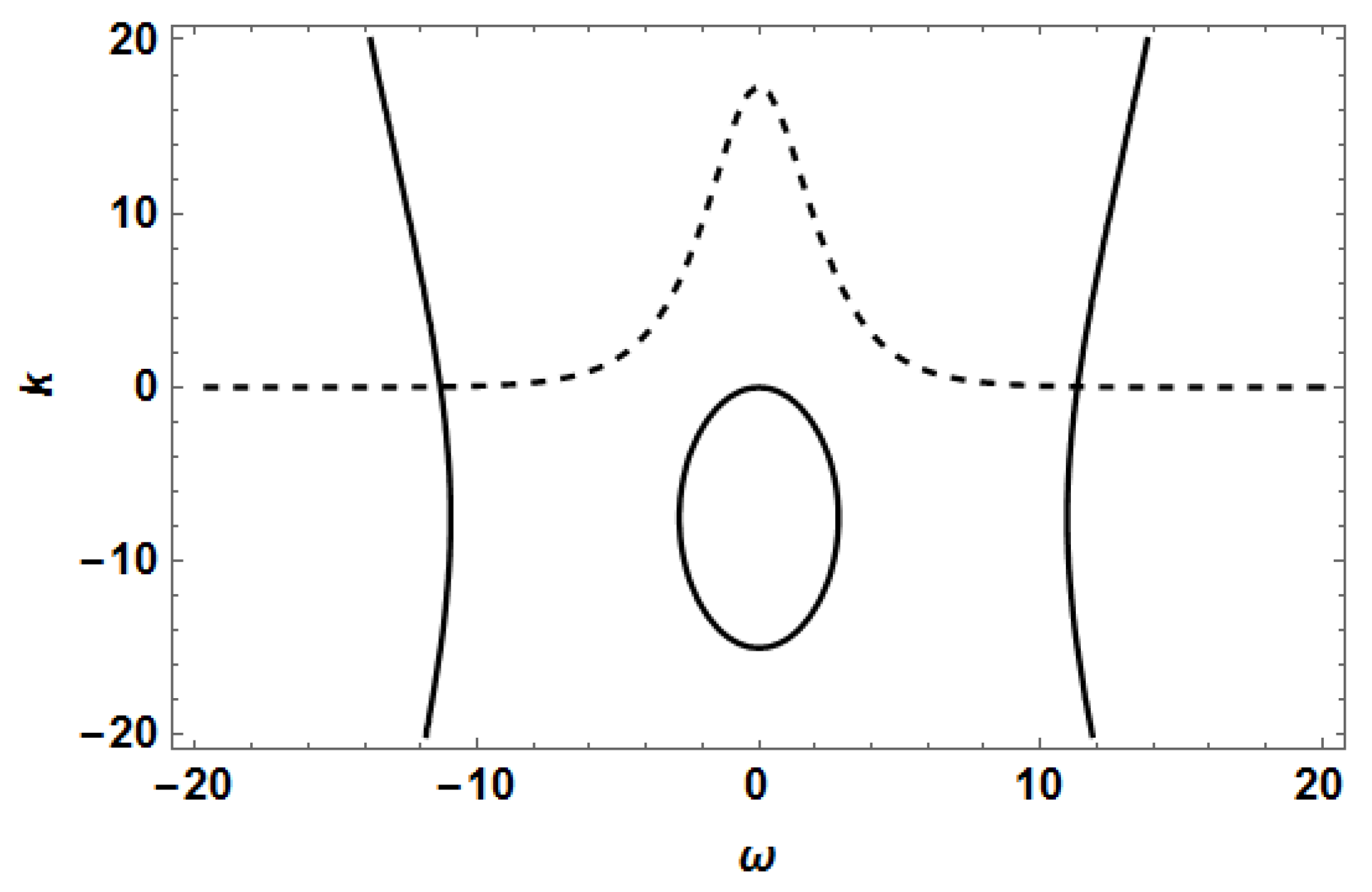
If we take the coefficients $c_0=1/40$, $c_2=1/2$ and $c_3=1/50$ in Equation (4), and the parameters $A=1$ and $B=1.5$ in Equation (42), the evolution of the pulse can be seen in Figure 7, which shows the form of $\left|u\left(z,t\right)\right|$ for $z=0.5$, 1.0 and 1.5. We do not see anything special in this figure, which is somewhat disappointing, since we expected an unusual behavior due to the awkward form of the dispersion relation $k\left(\omega \right)$ shown in Figure 2.

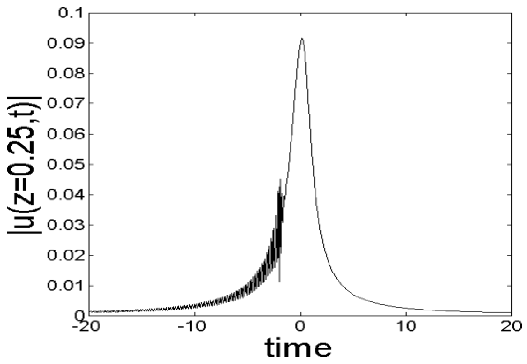
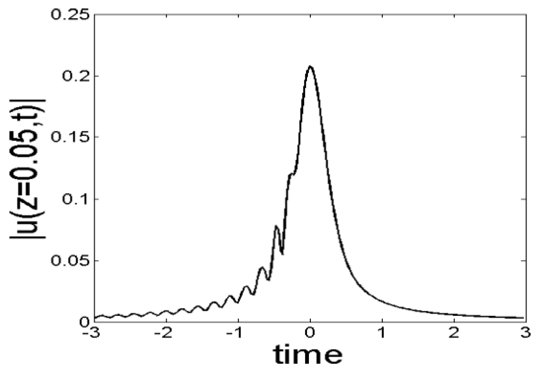
If we now obtain the solution of Equation (4) (with the same coefficients indicated above) and using again an initial condition of the form (42), but with $A=1/2$ and $B=14$, the result is more interesting. In this case small ripples are generated on the leading edge of the pulse (i.e., the left hand side of the pulse), as shown in Figure 8.

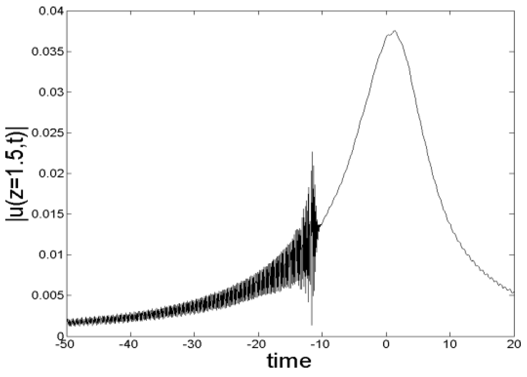
As the pulse advances along the fiber these ripples form a well-defined radiation wavetrain which propagates to the left of the pulse, as shown in Figure 9 and Figure 10.

At first sight, the radiation seen in Figure 9 might seem similar to the small-amplitude radiation waves emitted by solitary pulses which obey equations such as the following [1,2,11]:

$$i{u}_z+c_2{u}_{tt}-i{c}_3{u}_{ttt}+{\gamma }_1{\left|u\right|}^{2}u=0$$

(43)

$$i{u}_z+c_2{u}_{tt}+c_4{u}_{4t}+{\gamma }_1{\left|u\right|}^{2}u-{\gamma }_2{\left|u\right|}^{4}u=0$$

(44)

However, Figure 9 and Figure 10 show that the radiation emitted by the solution of Equation (4) possesses a unique characteristic, that no other model of optical pulses has ever predicted: the emission of radiation stops abruptly at a certain point along the retarded-time axis, and this point moves away from the pulse’s peak at a constant velocity. To understand clearly what this means we should remember that the independent variable “t” which appears in Equations (1), (4)–(8) and (26), and appears at the horizontal axes in Figure 8, Figure 9 and Figure 10, is not the laboratory time, but the so-called retarded time. Therefore, the graphs shown in Figure 8, Figure 9 and Figure 10 display the time-dependence of the square of the light intensity as measured by observers placed at different points (i.e., different values of z) along the optical fiber, but each of these observers has shifted his/her time origin in such a way that the time $t=0$ corresponds to the instant when the pulse’s maximum passes through the point z. Consequently, a graph such as the one shown in Figure 10 tells us that the radiation arrives at the observer placed at the position z before the arrival of the pulse. This implies that the radiation advances faster than the pulse. Moreover, it should be noticed that the point where we see an abrupt interruption of the radiation wave corresponds to the endpoint of the radiation wavetrain, since the first radiation waves that were emitted have already moved far away towards the left of the graph.

If we obtain numerical results similar to those shown in Figure 9 and Figure 10, but for $z=2$ and $z=2.5$, we can see that if the observer advances a distance $\Delta z=0.5$ along the optical fiber, the endpoint of the radiation wavetrain recedes to the left of the retarded time axis approximately $\Delta t\approx -5$, thus implying that this endpoint moves along the time axis with an “inverse velocity” $\Delta t/\Delta z\approx -10$. It might be worth emphasizing that in the study of light pulses along optical fibers the evolution variable is not the time, but the distance along the fiber, and therefore the “inverse velocity” $\Delta t/\Delta z$ is more adequate to describe the movement of radiation fronts (or pulses) such as those shown in Figure 9 and Figure 10, when they travel along the retarded time axis.

To understand why the end point of the radiation wave moves to the left of the retarded time axis with an inverse velocity $\Delta t/\Delta z\approx -10$ we must remember that the radiation emitted by optical pulses is usually the result of a resonance between these pulses and the small-amplitude radiation waves capable of traveling along the fiber. This resonance occurs when an optical pulse has a wavenumber $k_p$ that is contained in the range of wavenumbers permitted by the dispersion relation $k\left(\omega \right)$ of the system. In the case of Equation (4) we know that the dispersion relation is given by Equation (12), and the form of $k\left(\omega \right)$ is shown in Figure 2 for the coefficients $c_0=1/40$, $c_2=1/2$ and $c_3=1/50$. 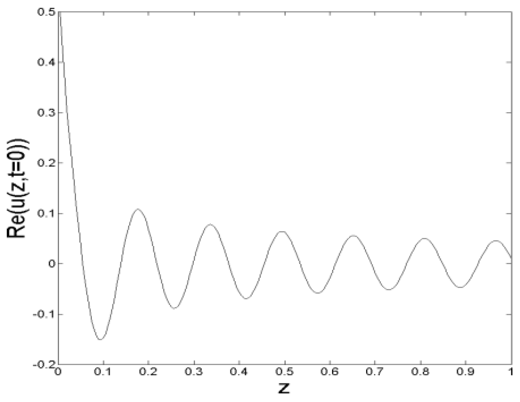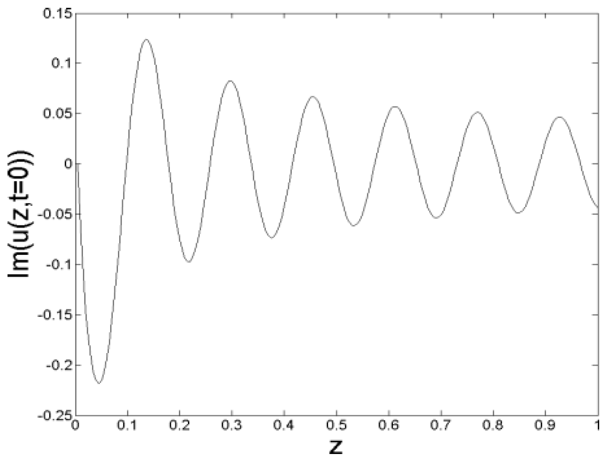What we do not know is the wavenumber corresponding to the solution of Equation (4) whose profiles are shown in Figure 8, Figure 9 and Figure 10. However, we can determine this wavenumber from the graphs of the real and imaginary parts of $u\left(z,t=0\right)$ shown in Figure 11 and Figure 12.

From these figures it follows that $k_p=-40$, and therefore a horizontal line placed at $k=-40$ intersects the dispersion relation $k\left(\omega \right)$ shown in Figure 2 at two points: $\left(k,\omega \right)=\left(-40, 0\right)$ and $\left(k,\omega \right)=\left(-40, 25\right)$. The first of these points does not correspond to a traveling wave (as its frequency is zero), but the second one corresponds to a linear wave with a resonant frequency $\omega =25$, phase velocity $k/\omega =-1.6$ and group velocity $dk/d\omega =-12.5$ (i.e., in fact we are talking of inverse velocities, $\Delta t/\Delta z$, as mentioned in the previous paragraph). We can see, therefore, that the endpoint of the radiation wavetrain that we see in Figure 9 and Figure 10 moves to the left of the retarded time axis at the group velocity corresponding to the resonant frequency $\omega =25$.

It should be noticed that the value $k_p=-40$, which we obtained from Figure 11 and Figure 12, could also be obtained from Equations (31) and (32). If we define $f\left(\omega \right)=c_3{\omega }^3-c_2{\omega }^2$, we can approximate $\sqrt{S\left(\omega \right)}\cong i\left(1+2c_{0}f\left(\omega \right)\right)$, and therefore Equation (31) implies that ${\lambda }_b\cong -i/c_0-if\left(\omega \right)$. Consequently, when $a\left(\omega \right)=0$, Equation (30) takes the form $U\left(z,\omega \right)=b\left(\omega \right)exp\left({\lambda }_{b}z\right)$, and from this equation it follows that $u\left(z,t\right)$ will contain the factor $exp\left(-iz/c_0\right)$, thus implying that $u\left(z,t\right)$ has a wavenumber $k_p=-1/c_0$. As we used $c_0=1/40$ to obtain Figure 11 and Figure 12, the origin of the value $k_p=-40$ is now clear.

We now understand the origin of the velocity of the endpoint of the radiation wavetrain shown in Figure 9 and Figure 10. However, we still do not know why this endpoint exists. In other words, we still do not know why the pulse stops emitting resonant radiation at a certain instant.

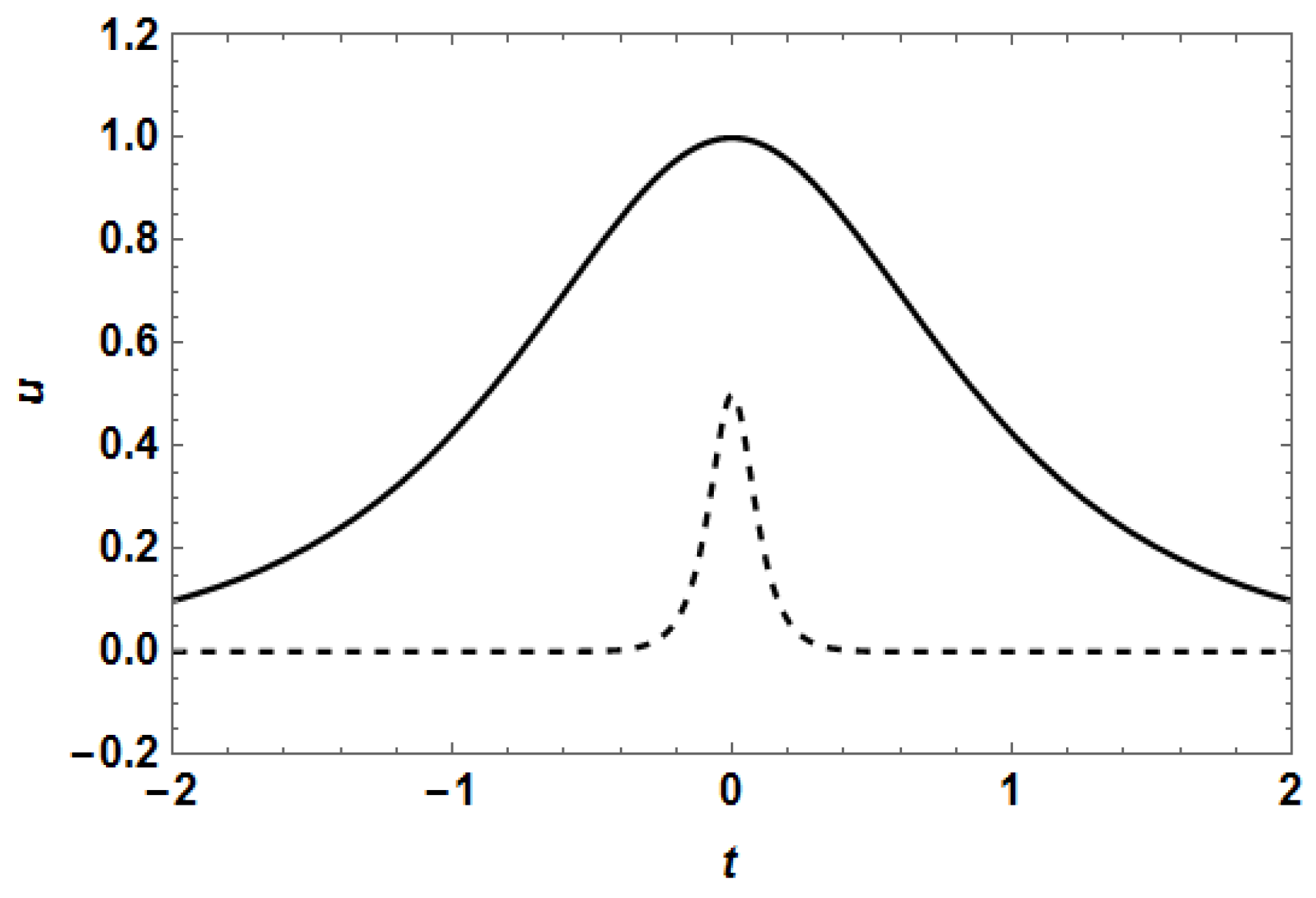
The clue to understand why the emission of radiation ends abruptly lies in the contrast between Figure 7 and Figure 10. Figure 7 shows no radiation at all, while in Figure 10 the radiation is quite conspicuous. The reason for this difference must be necessarily in the initial conditions used to obtain the solutions of Equation (4) which led to these two figures. 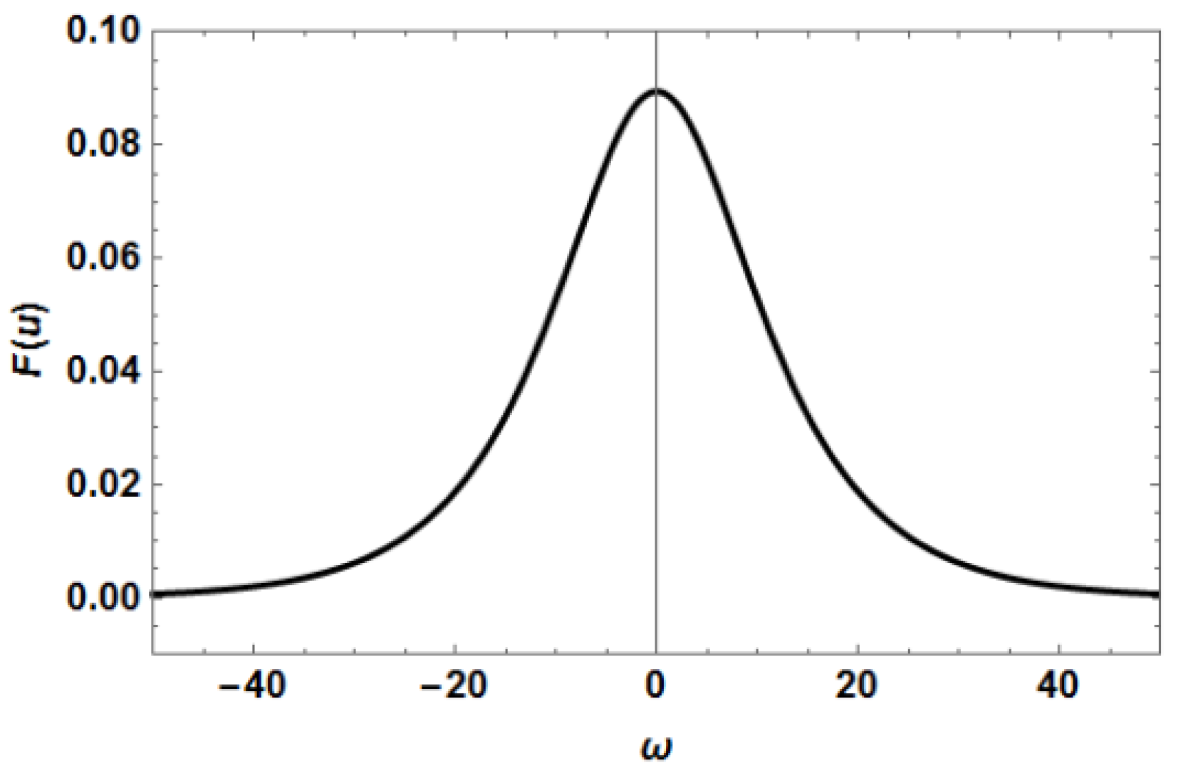These initial conditions are shown in Figure 13, and the absolute values of their Fourier transforms are shown in Figure 14 and Figure 15. 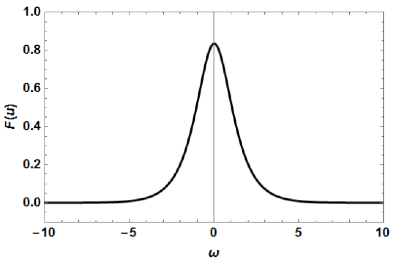We can see that the initial condition which lead to Figure 10 is much narrower than the initial condition corresponding to Figure 7, but the graphs which really suggest the answer to the presence of radiation in Figure 10, and its absence in Figure 7, are the Fourier transforms (FT) shown in Figure 14 and Figure 15.

The FT shown in Figure 14 shows that the spectrum corresponding to the initial condition which lead to Figure 7 is essentially contained in the interval $-5<\omega <5$, and it is practically zero for $\omega >{\omega }_3=10\left(1+\sqrt{2}\right)\approx 24.14$, which is the second interval where the dispersion relation $k\left(\omega \right)$ is well defined (remember, from Figure 2, that $k\left(\omega \right)$ is defined in two intervals: ${\omega }_1<\omega <{\omega }_2$ and $\omega >{\omega }_3$) Therefore, it is impossible for the initial condition which lead to Figure 7 to resonate with the linear waves with frequencies $\omega >{\omega }_3$, since this initial condition has no frequency components in this interval. On the contrary, the spectrum shown in Figure 15 shows that the initial condition which leads to Figure 10 contains significant frequency components with $\omega >{\omega }_3$. Consequently, when this initial pulse starts traveling along the fiber, it resonates with the linear wave with wavenumber $k_p=-40$ (the pulse’s wavenumber) and resonant frequency $\omega =25$, and thus the emission of radiation begins. However, the pulse’s width will begin to grow (and its spectrum will become narrower) as a result of the dispersive terms $c_2{u}_{tt}$ and $i{c}_3{u}_{ttt}$ which appear in Equation (4). As the dispersion of the pulse will continue indefinitely (since Equation (4) does not contain any nonlinear term which could cancel this dispersion), a moment will necessarily arrive when the pulse will be too wide, and its spectrum will be too narrow to have frequency components with $\omega >{\omega }_3$. Moreover, the components of the pulse with frequencies in the interval ${\omega }_2<\omega <{\omega }_3$ will die quickly, since the dispersion relation (shown in Figure 2) does not permit the propagation of linear waves with these frequencies. Therefore, a moment will arrive when the pulse´s spectrum will be essentially contained in the interval ${\omega }_1<\omega <{\omega }_2$ (where the dispersion relation allows the propagation of linear waves), and then the pulse will no longer be able to resonate with the wave with $\omega =25$ (the resonant frequency), and the emission of radiation will stop. So, the interruption of the radiation is due to the fact that the pulse’s spectrum is confined to live in the interval ${\omega }_1<\omega <{\omega }_2$ (far from the resonant frequency $\omega =25$), and the presence of the forbidden frequency gap ${\omega }_2<\omega <{\omega }_3$ seen in Figure 2 strongly contributes to this confinement.

We have thus seen that a very original consequence of having a dispersion relation given by an elliptic curve such as that shown on Figure 2 is the abrupt interruption of the resonant radiation emitted by a narrow pulse which obeys the linear Equation (4). Therefore, this novel radiation process is the consequence of the simultaneous presence of the non-slowly-varying-envelope term $u_{zz}$ and the third-order temporal derivative.

To close this sub-section it is worth observing that no qualitative changes are to be expected if we introduced the mixed derivative $u_{zt}$ in Equation (4). The equation thus obtained could be solved by Fourier transforms, just as we solved Equation (4). The form of the Equation (30) would still be valid, although the form of the functions ${\lambda }_{a,b}\left(\omega \right)$ and $S\left(\omega \right)$ would be slightly different. In this case (when we take into account a term of the form $c{u}_{zt}$ in Equation (4)), instead of Equations (31) and (32) we would have:

$${\lambda }_{a,b}=\frac{-i\left(1-c\omega \right)\pm \sqrt{S\left(\omega \right)}}{2c_0}$$

(45)

$$S\left(\omega \right)=-1-4c_0{c}_3{\omega }^3+\left(4c_0{c}_2-c^2\right){\omega }^2+2c\omega$$

(46)

It should be emphasized that the key ingredient which produces the peculiar radiation process shown in Figure 9 and Figure 10 is the presence of gaps of forbidden frequencies in the dispersion relation of Equation (4). It is interesting to investigate if these gaps survive if we introduce a term of the form $c{u}_{zt}$ in Equation (4). Therefore, let us consider the equation:

$$i{u}_z+c_0{u}_{zz}+c{u}_{zt}+c_2{u}_{tt}-i{c}_3{u}_{ttt}=0$$

(47)

and let us take the same coefficients $c_0=1/40$, $c_2=1/2$ and $c_3=1/50$ used to obtain Figure 7, Figure 8, Figure 9, Figure 10, Figure 11 and Figure 12. Concerning the coefficient $c$, one of the reviewers that revised this paper observed that in typical fibers $c<0$ and the absolute value of the ratio $c/c_0$ is approximately equal to the dimensionless number $\delta =2v_g^{-1}Z/T$, where Z and T are characteristic values of length and time, respectively, and $v_g^{-1}$ is the reciprocal group velocity. 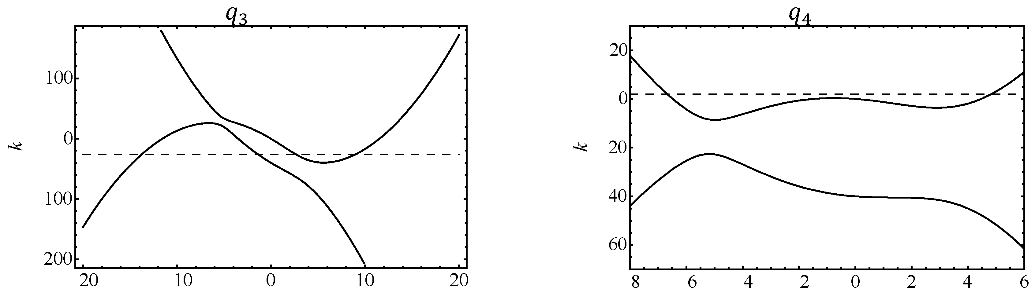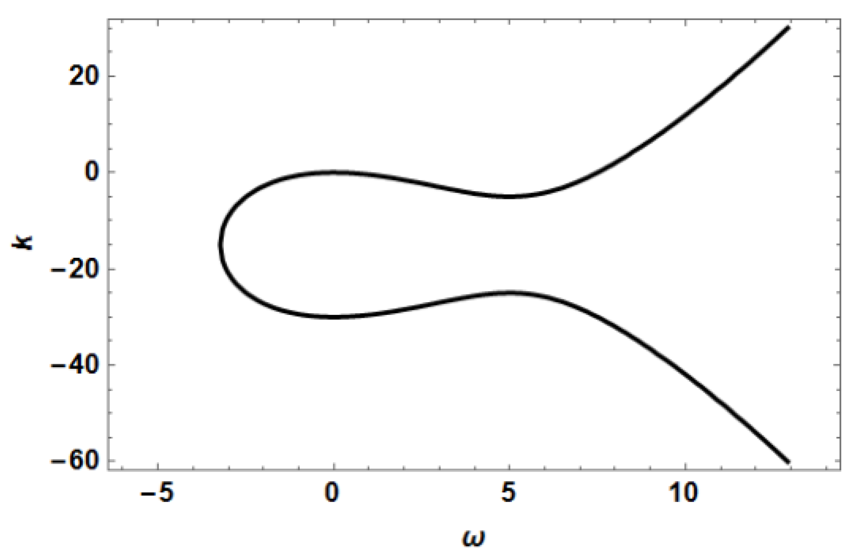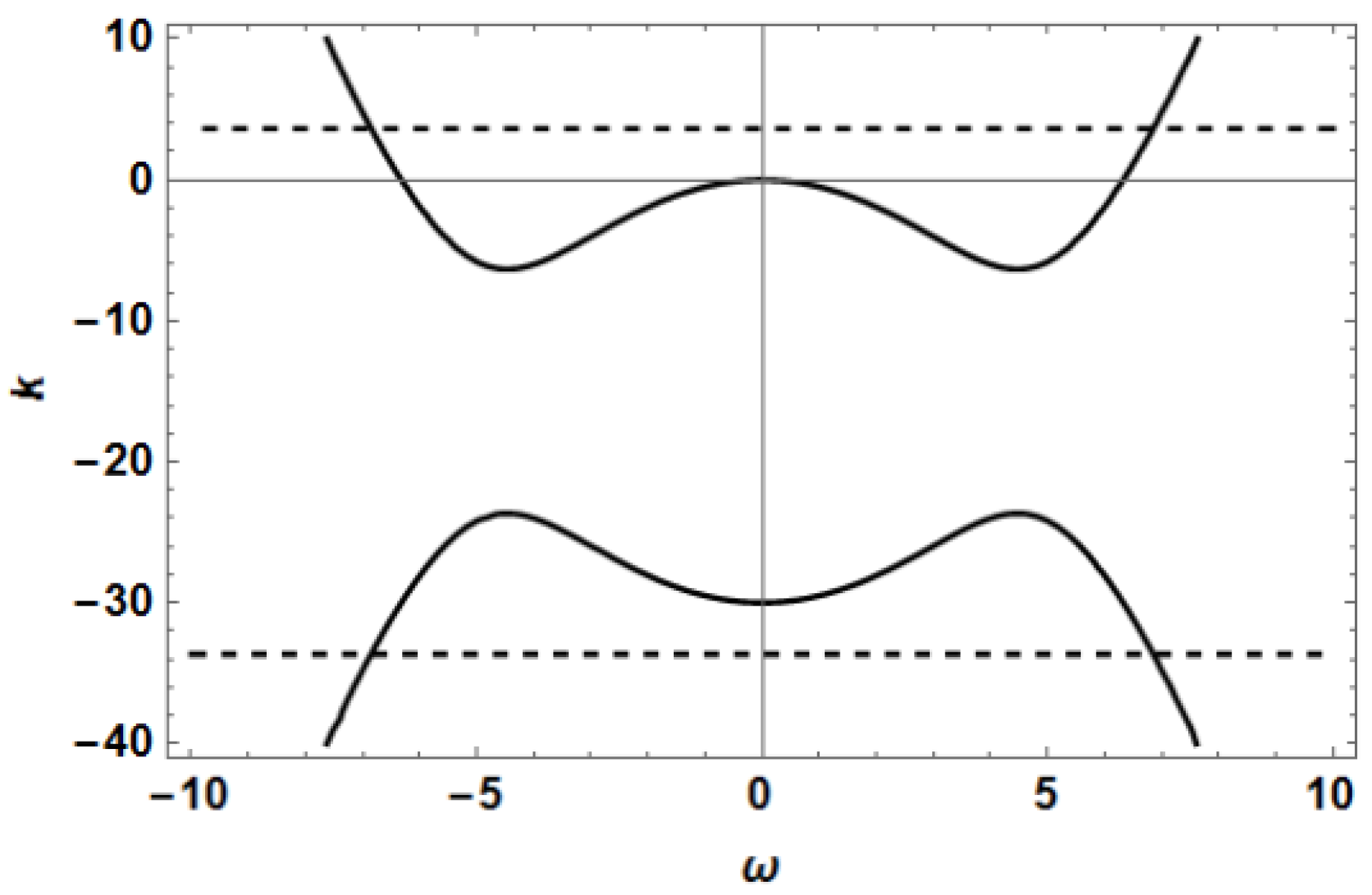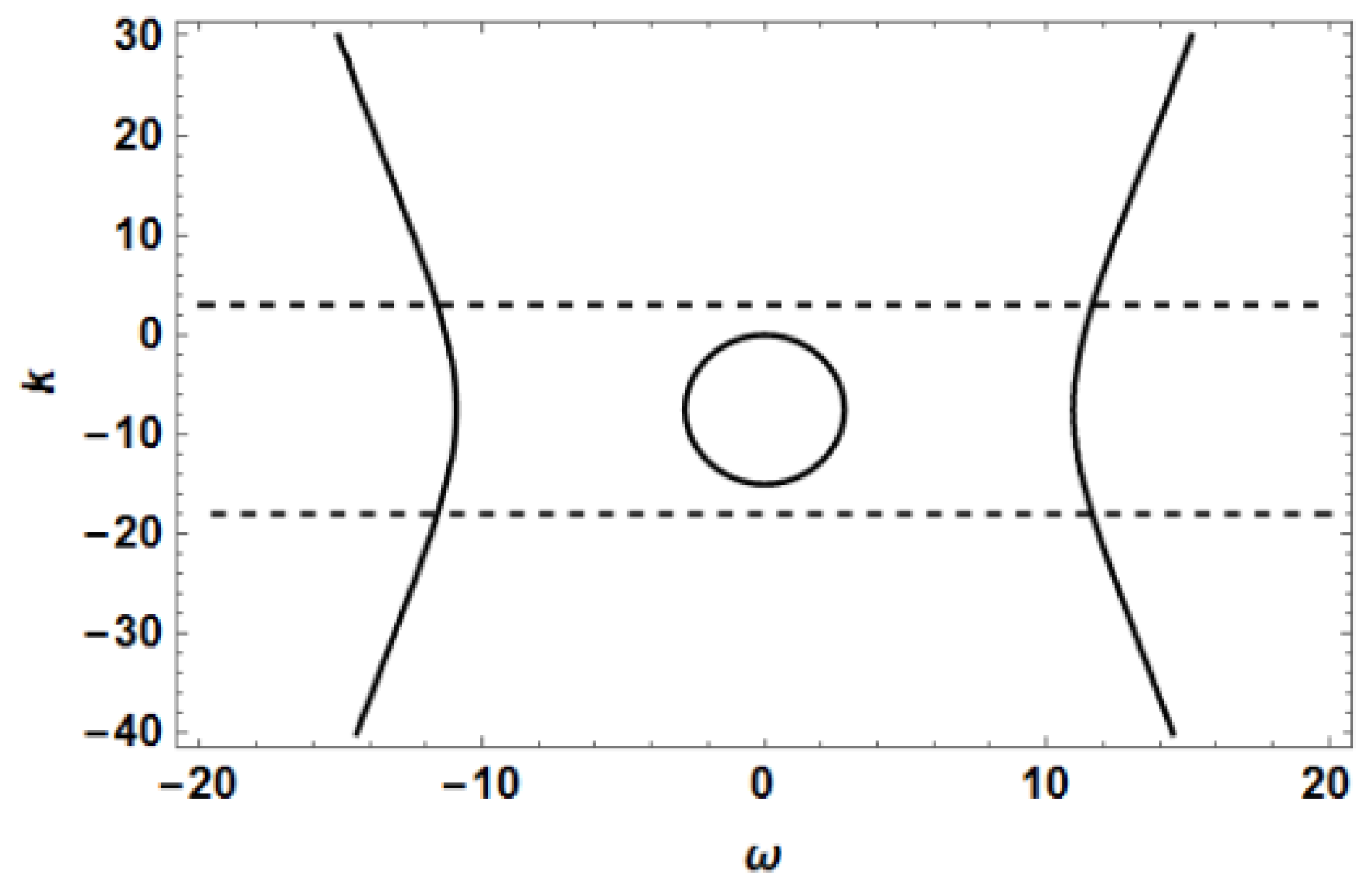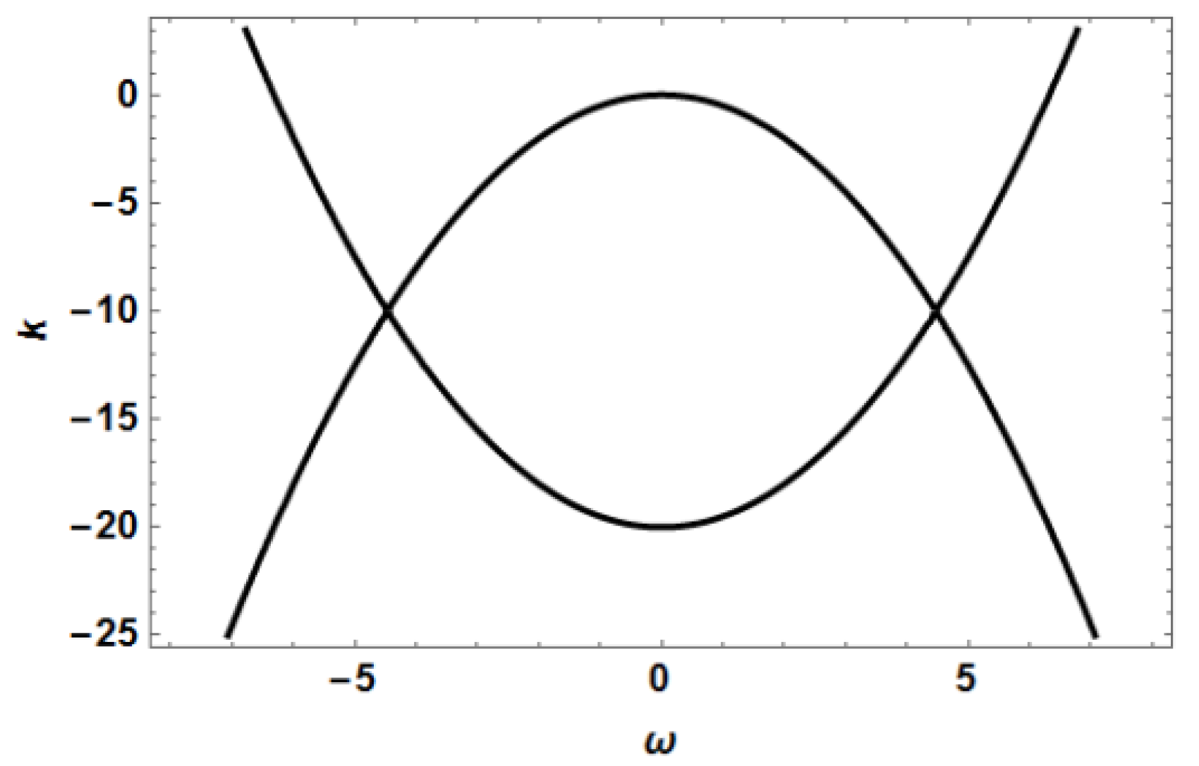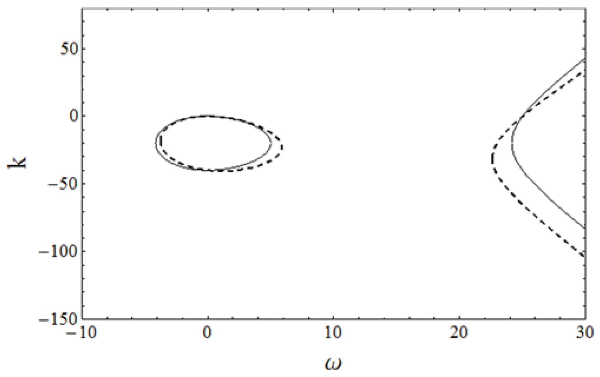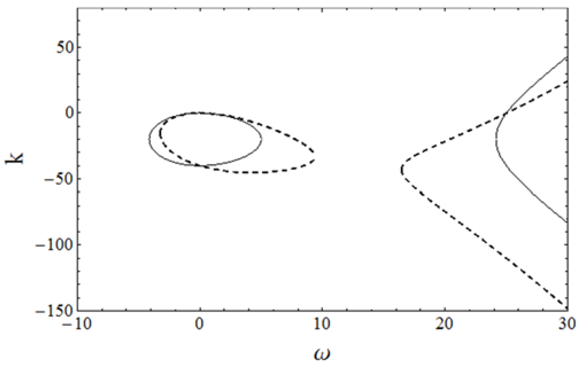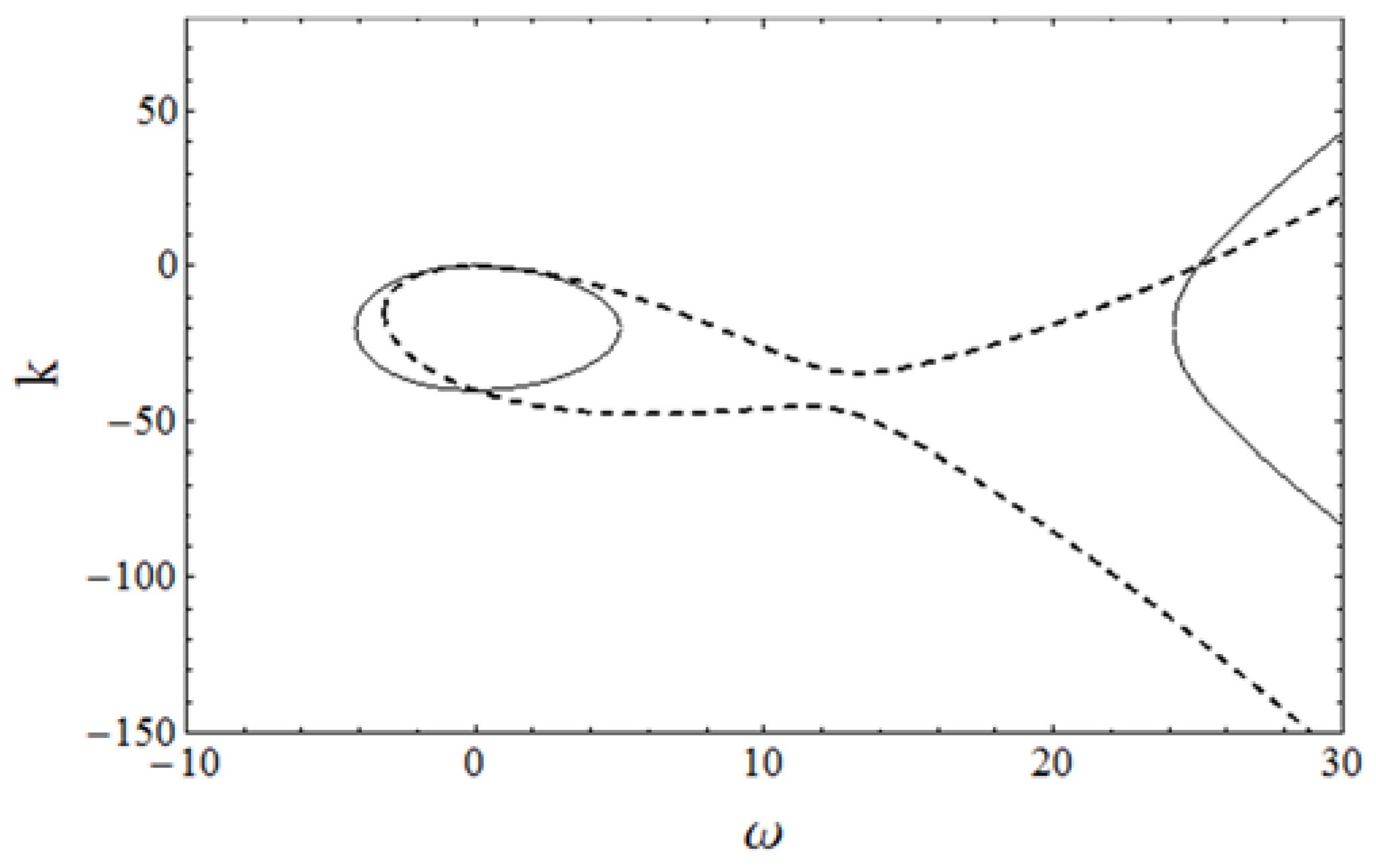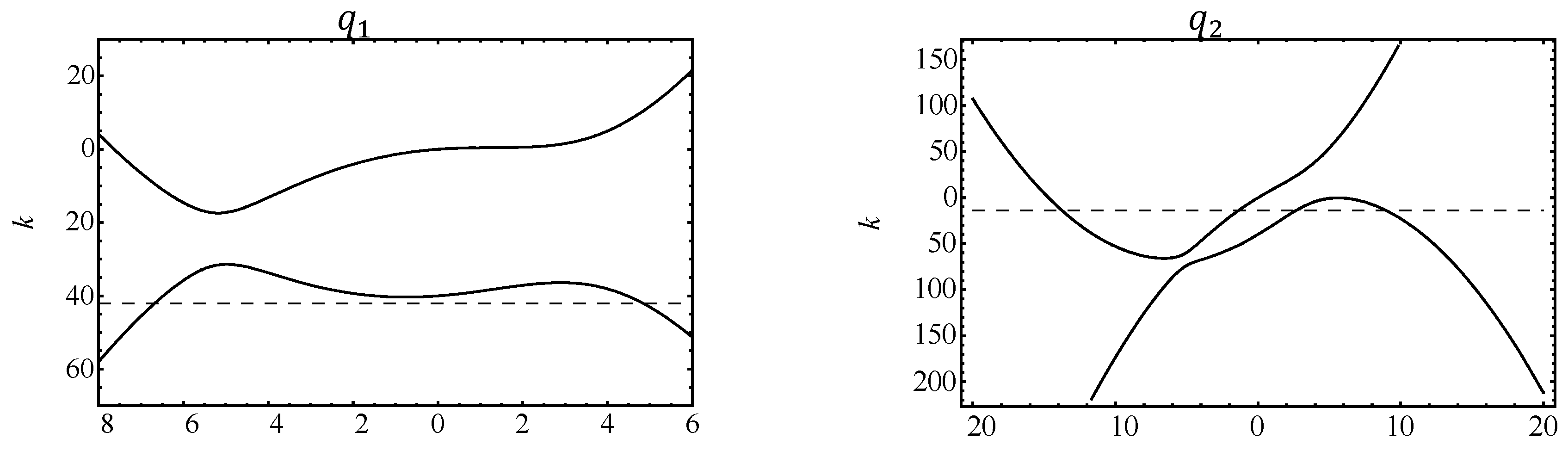In Figure 16, Figure 17, Figure 18 and Figure 19 the dashed curves show the form of the dispersion relation of Equation (47) for three different values of $c$ ($-c_0$, $-2.8 c_0$ and $-3.2 c_0$), and the continuous curve shows the dispersion relation when the term $c{u}_{zt}$ is absent.

We can see that the finite gap of forbidden positive frequencies survives in Figure 16 and Figure 17, but it disappears in Figure 18. Therefore, the presence of the term $c{u}_{zt}$ in Equation (47) modifies the gaps of forbidden frequencies in a significant way. In fact, the gap of forbidden positive frequencies will disappear if the coefficients $c$, $c_0$, $c_2$ and $c_3$ are such that the equation $S\left(\omega \right)=0$ has only one real root ($S\left(\omega \right)$ being the polynomial shown in Equation (46)). In particular, for pulses propagating in a typical optical fiber with a group velocity $v_g\cong 0.68c_L$ ($c_L$ being the light speed in vacuum) the band of forbidden frequencies may not exist for processes whose characteristic dimensions are $Z\cong 1 \mathrm{mm}$ and $T\cong 1 \mathrm{ps}$, as for these values $\delta \approx 10$, and Figure 16, Figure 17 and Figure 18 show that the band of forbidden frequencies does not exist if $\delta \ge 3.2$ (and $c_0$, $c_2$ and $c_3$ have the values used to obtain Figure 16, Figure 17 and Figure 18). However, the value of $\delta$ might be smaller in special fibers where $v_g$ is closer to $c_L$ (as in photonic fibers with air holes), and we consider processes where $Z/T$ is also closer to $c_L$. In such conditions the band of forbidden frequencies might exist. In fact, the generation of a band of forbidden frequencies has already been observed by Fang et al. [38] during the propagation of very short optical pulses in photonic crystal fibers, a result that Fang et al. considered “the most distinctive feature” of this process.

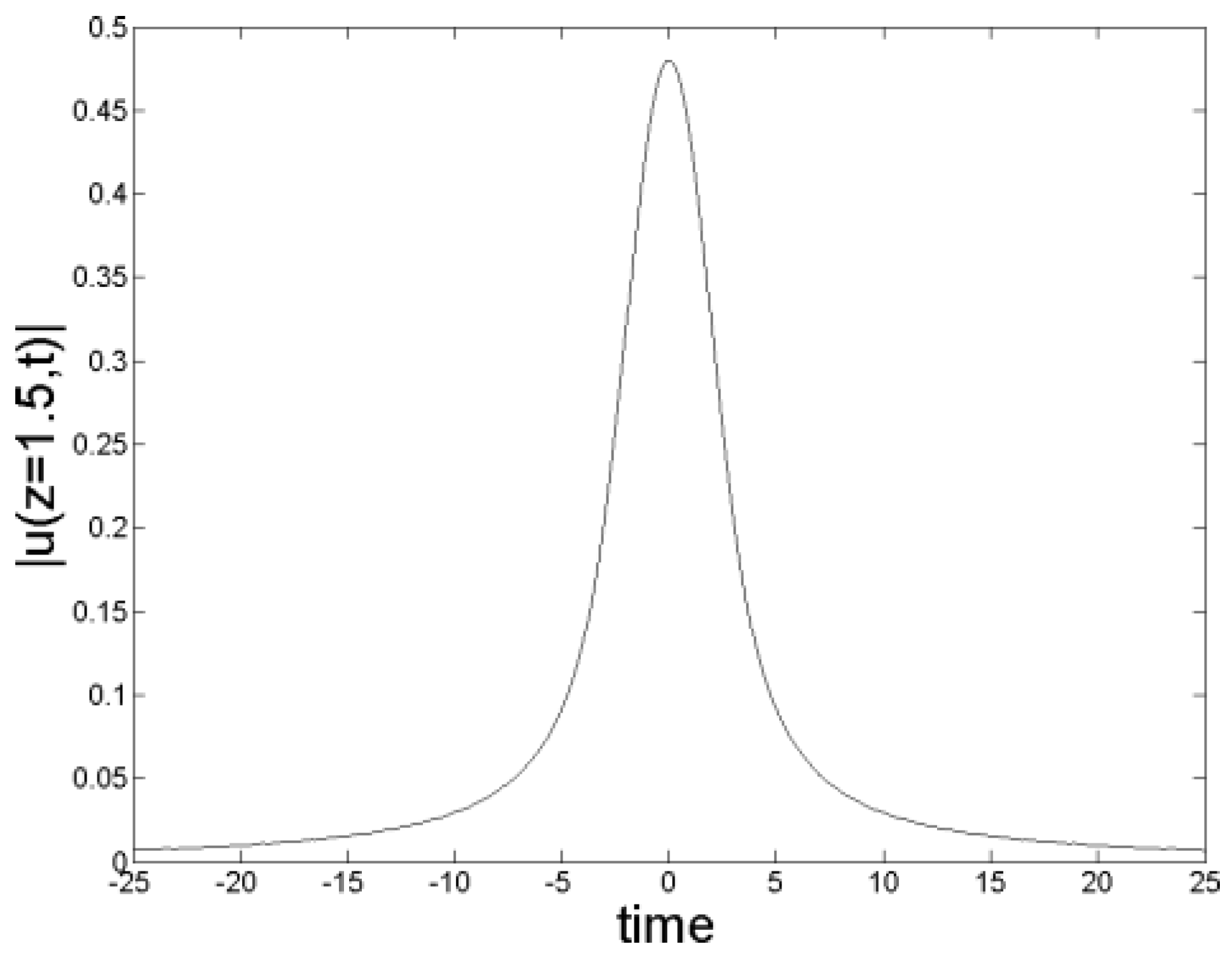
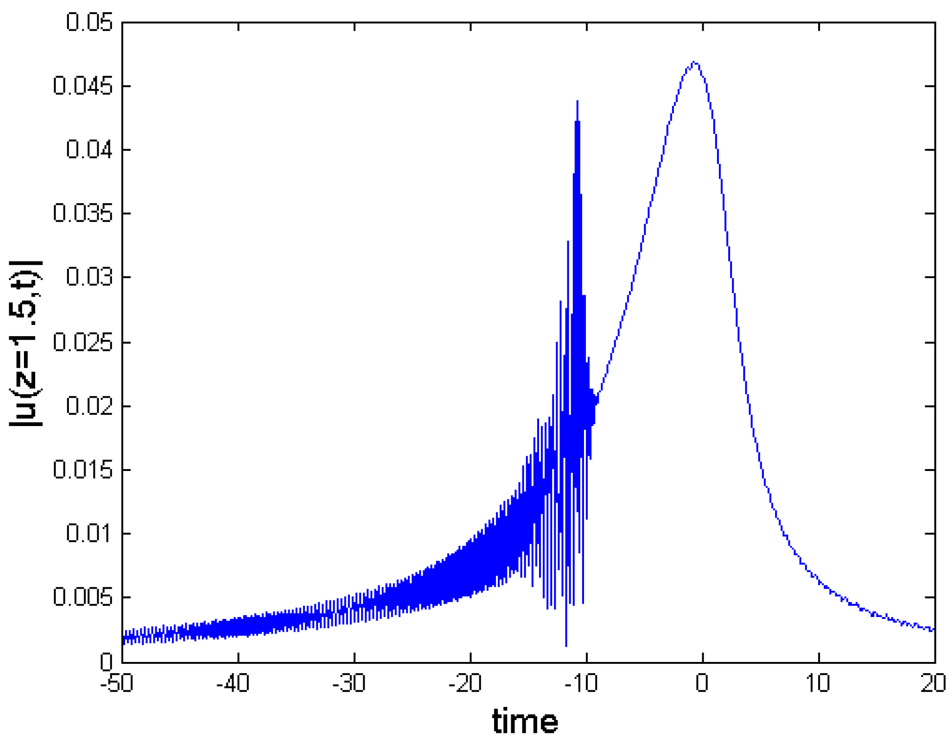
It might be interesting to see how pulses evolve when the width of the band of forbidden frequencies shrinks, as in the dispersion relation shown by the dashed curve in Figure 17. In Figure 19 we can see the modulus of the solution (at $z=1.5$) of Equation (47) corresponding to a narrow initial pulse of the form (42), with $A=1/2$ and $B=14$, and the coefficients used to obtain the dashed curve in Figure 17.

We can see that the graph shown in Figure 19 is similar to that shown in Figure 10, but the amplitude of the radiation is significantly higher. However, the radiation also stops at a definite time (as in Figure 10), due to the presence of the band of forbidden frequencies shown in Figure 17.

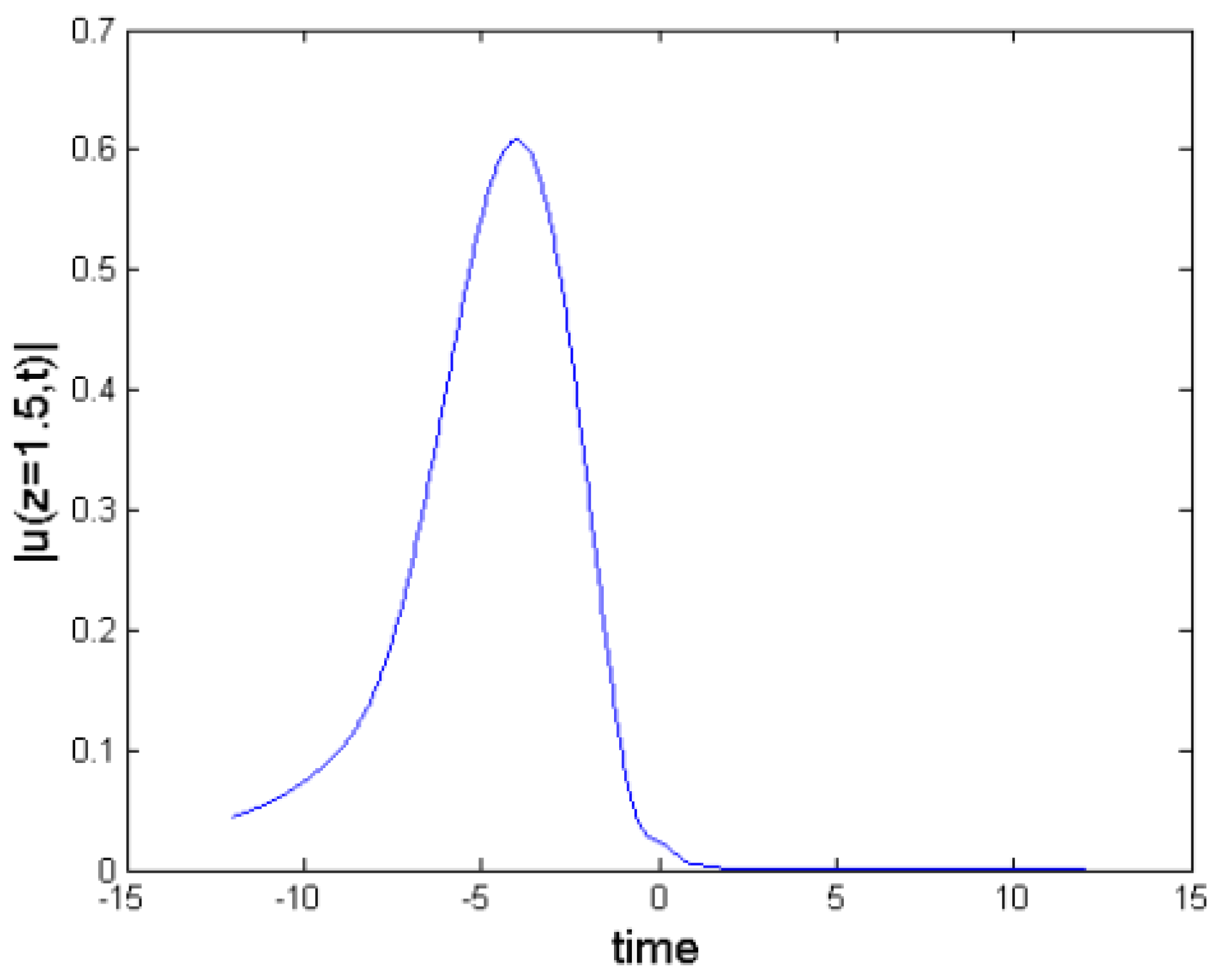
If we now calculate the solution of Equation (47) corresponding to the broader initial condition used to obtain Figure 7, and the same coefficients used in Figure 19, we obtain Figure 20. This figure shows that the pulse does not emit any radiation at all, as expected, since the initial condition is now a broad pulse, and its Fourier transform is too narrow to have frequency components which may resonate with the small-amplitude linear waves corresponding to the right branch of the dispersion relation seen in Figure 17. Figure 20 also shows that the position of the pulse has been shifted to the left, a result that is due to the presence of the term $c{u}_{zt}$ in Equation (47), and the negative value of the coefficient $c$ (Figure 7 shows that the pulse does not move to the left when the term $c{u}_{zt}$ is absent).

3.3. Solutions of Equation (5)

Now let us investigate how the solutions of Equation (5) behave. As we saw in Figure 4, when the coefficients $c_0$, $c_2$ and $c_4$ satisfy the condition (17), the dispersion relation presents two finite bands of forbidden frequencies (defined in (22)). Therefore, we expect that narrow solitons will exhibit a behavior similar to that of the solutions of the Equation (4). More precisely, we expect that if take an initial condition whose Fourier transform (FT) is wide enough to contain significant frequency components in the intervals $\omega <-{\omega }_2$ and $\omega >{\omega }_2$, the pulse will start radiating, but the radiation will stop at some time, when the pulse widens and its FT becomes too narrow. To verify this expectation we obtained the numerical solution of Equation (5) with coefficients $c_0=1/15$, $c_2=1/2$ and $c_4=1/256$, and using an initial condition $u\left(0,t\right)$ of the form (42) with $A=1$ and $B=7$. As in the case of Equation (4), we can obtain the solution of Equation (5) by calculating the Fourier transform (FT) of this equation, and the FT of the solution also has the form shown in Equation (30), with ${\lambda }_{a,b}\left(\omega \right)$ given by Equation (31), but with the function $S\left(\omega \right)$ which appears within the square root now defined as follows:

$$S\left(\omega \right)=-1-4c_0\left(c_4{\omega }^4-c_2{\omega }^2\right)$$

(48)

As this function is positive on two regions of the $\omega$ axis, the function $U\left(z,\omega \right)$ (given in Equation (30)) would grow exponentially in z, unless we impose the restriction $a\left(\omega \right)=0$. This restriction implies that Equation (41) is also valid in this case (but using Equation (48) in the expression (31) which defines the function ${\lambda }_b\left(\omega \right)$). 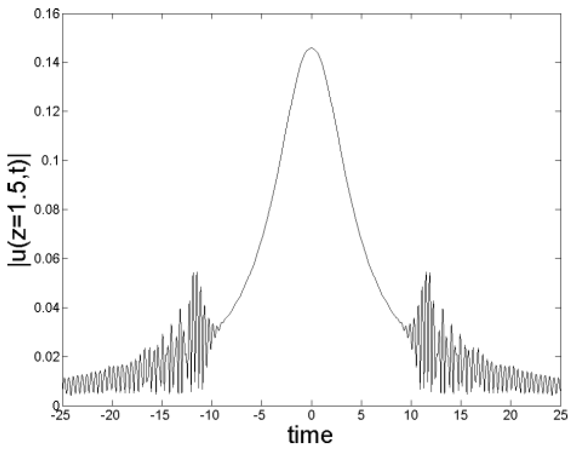Therefore, to solve Equation (5) we used $u\left(0,t\right)$ as defined in Equation (42), and we calculated $u_z\left(0,t\right)$ with Equation (41). In Figure 21 we can see the profile of $\left|u\left(z=1.5,t\right)\right|$ corresponding to the initial condition (42) with $A=1$ and $B=7$. As expected, we see that the pulse starts emitting radiation, but afterwards the radiation stops. The only important difference in comparison with the behavior of the solutions of Equation (4) is that the solution of Equation (5) emits radiation in both directions, due to the fact that its dispersion relation, shown in Figure 4, is now symmetrical with respect to the wavenumber axis.

On the other hand, in Figure 22 we can see the profile of another solution of Equation (5) corresponding to an initial condition of the form (42), but now using $A=1$ and $B=2$ (and the same coefficients $c_0$, $c_2$ and $c_4$). In this case no radiation is observed because the initial pulse was very wide, and its FT was very narrow, and therefore the initial FT has no significant frequency components in the intervals $\omega <-{\omega }_2$ and $\omega >{\omega }_2$ (where the resonant frequencies are located).

We have thus seen that the behavior of the radiating pulses of Equations (4) and (5) is similar, except that the solutions of Equation (5) emit radiation in both directions, and those of Equation (4) only radiate to the left. However, Equations (4) and (5) differ in a significant aspect. In the case of Equation (4) the function $S\left(\omega \right)$ defined by Equation (32) is always positive in a portion of the real axis, and consequently is always necessary to impose the restriction $a\left(\omega \right)=0$ which leads to the relationship between $u\left(0,t\right)$ and $u_z\left(0,t\right)$ given by Equation (41). On the other hand, in the case of Equation (5), depending on the values of the coefficients $c_0$, $c_2$ and $c_4$, the function $S\left(\omega \right)$ defined by Equation (48) may be positive over certain frequency intervals, and in these cases the restriction $a\left(\omega \right)=0$ is necessary, and the Equation (41) again defines a necessary relation between $u\left(0,t\right)$ and $u_z\left(0,t\right)$. However, for certain coefficients, the function $S\left(\omega \right)$ might be always negative, and then the values of the functions ${\lambda }_{a,b}\left(\omega \right)$ would be imaginary for all frequencies. In these cases there is no reason to impose the restriction $a\left(\omega \right)=0$, and with the disappearance of this restriction also the relations (40) and (41) disappear. Therefore, in the case of Equation (5), when ${\lambda }_a$ and ${\lambda }_b$ are both imaginary, we face again the question: how do we specify the initial condition $u_z\left(0,t\right)$? In the following paragraph we address this question.

When $a\left(\omega \right)\ne 0$ the Equations (40) and (41) no longer hold, but we can obtain an approximate relation between $u_z\left(0,t\right)$ and $u\left(0,t\right)$ by considering what happens when we send a light pulse at the beginning of an optical fiber. As the pulse enters into the fiber, the wavelength of the carrier wave changes (since the light’s velocity is different inside the fiber), and this change introduces a factor $\exp \left(i\Delta k z\right)$ in the mathematical form of the pulse. In other words, at the beginning of the fiber (inside the fiber, near the point $z=0$) the form of the light pulse will be:

$$u\left(z,t\right)=f\left(t\right) e^{i\Delta k z}$$

(49)

where $f\left(t\right)$ defines the temporal profile of the pulse. Consequently, from Equation (49) it follows that:

$$u_z\left(0,t\right)=i\Delta k u\left(0,t\right)$$

(50)

and this equation, whose FT is similar to Equation (40), implies that the form of the function $u\left(0,t\right)$ determines the form of $u_z\left(0,t\right)$. It should be noticed, however, that we do not know the value of the parameter $\Delta k$. This parameter depends on the exact form of the refractive index of the fiber as a function of the light intensity. However, if we approximate the wavelength of the light inside the fiber in the form $\lambda \cong {\lambda }_0/n_0$, where ${\lambda }_0$ is the wavelength outside the fiber, and $n_0$ is the intensity-independent part of the refractive index, then we can approximate $\Delta k$ in the form:

$$\Delta k\cong 2\pi \left(n_0-1\right)/{\lambda }_0$$

(51)

Therefore, when there is no justification for using Equation (41) to calculate $u_z\left(0,t\right)$, this function might be calculated by means of the approximate Equations (50) and (51). In fact, in the following section we will see that the exact soliton solutions of Equation (6) are indeed consistent with a linear relationship between $u_z\left(0,t\right)$ and $u\left(0,t\right)$, such as that given by Equation (50).

To close this section, it is important to emphasize that the peculiar radiation behavior observed in Figure 9, Figure 10, Figure 19 and Figure 21 is a direct consequence of the presence of bands of forbidden frequencies in the dispersion relations of Equations (4), (5) and (47), and these forbidden bands are the result of the interplay between the non-SVEA tem $u_{zz}$ and higher-order dispersive terms such as $-i{u}_{ttt}$ or $u_{4t}$. Therefore, the principal lesson to be learnt from the study of Equations (4), (5) and (47) is the following: when a very short pulse is launched along an optical fiber, some of the frequencies which are contained in the initial pulse may not be permitted to travel along the fiber, since bands of forbidden frequencies may appear in the dispersion relation of the equation which controls the propagation of the pulse. Although these forbidden bands may be cancelled by the influence of the term $c{u}_{zt}$ (which we did not include in Equations (4) and (5)), a band of this type has already been observed in a photonic crystal fiber, as mentioned before [38].

4. The Nonlinear Equations (6)–(8)

In this section we will show that the nonlinear Equations (6)–(8) have exact soliton solutions of different forms, some of them being embedded solitons (as we shall explain in the following).

4.1. The Solitons of Equation (6)

Equation (6) is an interesting generalization of Equation (5) because it accepts soliton solutions of two different types. The first of these solutions is the following:

$$u\left(z,t\right)=A \mathrm{sech}\left(Bt\right) e^{iCz}$$

(52)

where A, B and C are the following constants:

$$B^2=\frac{{\gamma }_1}{20c_4}{\left(\frac{24c_4}{{\gamma }_2}\right)}^{1/2}-\frac{c_2}{10c_4}$$

(53)

$$A={\left(\frac{24c_4}{{\gamma }_2}\right)}^{1/4}B$$

(54)

$$C={\left(2c_0\right)}^{-1}\left[-1\pm \sqrt{1+4c_0\left(c_4{B}^4+c_2{B}^2\right)}\right]$$

(55)

Equation (55) defines two values for C, and consequently Equation (6) has two solutions of the form (52) with different wavenumbers $C_1$ and $C_2$ corresponding, respectively, to the signs “plus” and “minus” in front of the radical that appears in Equation (55).

It is worth observing that the solution defined by Equations (52)–(55) is the particular solution of Equation (6) corresponding to the initial conditions:

$$u\left(0,t\right)=A \mathrm{sech}\left(Bt\right)$$

(56)

$$u_z\left(0,t\right)=iC u\left(0,t\right)$$

(57)

with A, B and C given by Equations (53)–(55). We can see that Equation (57) has the same form as Equation (50), but with a particular value of the wavenumber. Therefore, the use of initial conditions of the form (50) in order to look for particular solutions of Equations (5) and (6) seems justified.

We must now remember that in Section 2 we saw that if the inequality (17) holds, the range of wavenumbers permitted by the linear dispersion relation of Equation (6) (given by Equation (15) or, alternatively, by Equation (21)), covers the entire real axis, and consequently, in this case (when $c_0{c}_2^2>c_4$) the soliton wavenumbers $C_1$ and $C_2$ are obviously contained within the range of wavenumbers permitted by the linear dispersion relation of the system. This characteristic implies that these solitons are not standard ones (since standard solitons have wavenumbers lying outside the linear spectrum of the system), but they are embedded solitons. It is worth remembering that prior to 1997 it was believed that soliton wavenumbers must necessarily lie outside the linear spectra of the systems. Otherwise (it was believed) the solitons would resonate with the small-amplitude linear waves capable of propagating in the system, and the solitons would emit resonant radiation. However, in 1997 it was discovered that exact radiationless soliton solutions with wavenumbers contained within the range of the linear dispersion relation of the system may indeed exist [11], and the term “embedded soliton” was coined two years later to distinguish these peculiar solitons from the standard ones [45,46].

In Figure 4 we showed the form of the dispersion relation, given by Equation (21), in the particular case when $c_0=1/15$, $c_2=1/2$ and $c_4=1/256$. This figure also shows the position of the soliton wavenumbers, $C_1$ and $C_2$, given by Equation (55) with ${\gamma }_1=5$ and ${\gamma }_2=1$. If we look at this figure an interesting question arises: how is the frequency spectrum of the exact soliton solution (52) in comparison to the dispersion relation? To answer this question, in Figure 23 we have superimposed the Fourier transform (FT) of the exact soliton (52) and the scaled dispersion relation $k\left(\omega \right)/8.6287$. The scaling factor (8.6287)⁻¹ was introduced for the amplitude of the FT and the scaled dispersion relation to have the same size at $\omega =0$. This figure shows that the amplitude of the spectrum of the exact soliton solution is completely insignificant in the range of frequencies where the lateral branches of the dispersion relation are placed. Therefore, even though the two soliton solutions of Equation (6) have wavenumbers $C_1$ and $C_2$ that intersect these branches (as the dashed lines show in Figure 4), and this fact favors a resonance between the solitons and the radiation modes, the soliton spectrum is practically zero at the frequencies where $k\left(\omega \right)=C_{1,2}$, thus implying that the solitons do not have frequency components capable of resonating with the radiation modes satisfying the resonance condition $k\left(\omega \right)=C_{1,2}$.

This qualitative argument is helpful to understand why these embedded solitons do not resonate with the radiation modes, in spite of the fact of having wavenumbers contained in the range of the dispersion relation. However, if desired, it is also possible to use the procedure shown in Refs. [18,20] to construct a rigorous proof (not just a qualitative one) which shows that the absence of resonances between the solitons and the radiation modes is the consequence of a delicate balance between the linear and the nonlinear terms of Equation (6). This procedure consists in taking the FT of Equation (6), using a function of the form (52) to calculate the FT of the nonlinear terms. In this way, an expression for the FT of $u\left(z,t\right)$ is obtained, which contains a quotient of two polynomials in $\omega$. The polynomial in the numerator depends on the nonlinear coefficients, and that in the denominator depends on the coefficients of the linear terms. Moreover, the roots of the polynomial that appears in the denominator determines the resonant frequencies. The next step is to prove that if the values of the parameters A, B and C which appear in (52) have the values given by the Equations (53)–(55), then the two polynomials cancel out, and the denominator disappears. With the disappearance of this denominator, the possibility of a resonance also disappears, thus explaining why the solution given by Equations (52)–(55) does not resonate with the radiation modes.

The above paragraph shows that the soliton solutions of Equation (6) (defined by Equations (52)–(55)) are embedded solitons if the inequality (17) holds. On the other hand, when the inequality (18) holds, the linear dispersion relation (21) presents a band of forbidden wavenumbers (defined by (19) and (20)), and in this case it is not evident if the soliton wavenumbers $C_1$ and $C_2$ are located within the forbidden band (in which case the solitons would be standard), or they lie outside this band (and they are contained within the linear spectrum of the system), in which case they would be embedded solitons. A careful comparison of the soliton wavenumbers $C_1$ and $C_2$ given by Equation (55), and the boundaries $k_1$ and $k_2$ of the band of forbidden frequencies (given by Equation (20)), show that:

$$C_2>k_2 \mathrm{and} C_1<k_1$$

(58)

These inequalities imply that the soliton wavenumbers lie outside the forbidden band $k_1<k<k_2$, and consequently there are contained within the range of wavenumbers permitted by dispersion relation, thus implying that also in this case (when the inequality (18) holds) the solitons defined by Equations (52)–(55) are embedded solitons. In Figure 3 we showed the dispersion relation $k\left(\omega \right)$ defined by Equation (15) when $c_0=1/30$, $c_2=1/2$ and $c_4=1/80$, and the dashed horizontal lines show the position of the soliton wavenumbers $C_1$ and $C_2$ (corresponding to ${\gamma }_1=5$ and ${\gamma }_2=1$), evidencing that these wavenumbers lie outside the forbidden band.

Now let us consider the second type of soliton solutions of Equation (6). Direct substitution shows that if the coefficients of the equation satisfy the following relation:

$${\gamma }_1^2{c}_4=-\frac{18}{7} {\gamma }_2{c}_2^2$$

(59)

then Equation (6) has an exact solution of the following form:

$$u\left(z,t\right)=F \mathrm{sech}\left(Gt\right)e^{i\left[Pz+Q ln\left\{\cosh \left(Gt\right)\right\}\right]}$$

(60)

where:

$$F^2=-\frac{9}{4}\frac{c_2^2}{{\gamma }_1{c}_4}$$

(61)

$$G^2=\frac{c_2}{8c_4}$$

(62)

$$Q=\pm \sqrt{5}$$

(63)

and P is the solution of:

$$c_0{P}^2+P+\frac{9c_2^2}{16c_4}=0$$

(64)

which, if $c_0\ne 0$, implies that:

$$P={\left(2c_0\right)}^{-1}\left[-1\pm \sqrt{1-9c_0{c}_2^2/\left(4c_4\right)}\right]$$

(65)

The solution given by Equations (60)–(65) is an interesting one, as it contains an unusual nonlinear frequency shift. This type of frequency shift was also found in [17], and if $c_0=0$ our Equations (59)–(64) coincide with the results found in this reference.

It should be noticed that Equation (6) does not accepts simultaneously the solutions (52) and (60). The solution (52) exists for certain values of the coefficients $c_0$, $c_2$, $c_4$, ${\gamma }_1$ and ${\gamma }_2$, and the solution (60) exists for other values of these coefficients. For example, if $c_2$ and $c_4$ are both positive, the solution (52) only exists if ${\gamma }_1$ is also positive (as a consequence of Equation (53)), while the solution (60) will only exist if ${\gamma }_1$ is negative (as a consequence of Equation (61)).

The existence of two different types of solitons in Equation (6) suggests that this equation might have additional exact analytical solutions. It would be interesting to investigate if the new methods described in Refs. [47,48,49] and the references therein, might be successful in finding new solutions for Equation (6).

4.2. The Solitons of Equation (7)

Direct substitution shows that Equation (7) has moving soliton solutions of the following form:

$$u\left(z,t\right)=R sech\left(\frac{t-Vz}{W}\right) e^{i\left(qz-rt\right)}$$

(66)

where r, q, V, R and W are constants whose values can be calculated as explained in the following. First we calculate r:

$$r=-\frac{c_3}{4c_4}$$

(67)

and then we define the following parameters:

$$Y=c_4{r}^4+c_3{r}^3-c_2{r}^2$$

(68)

$$M=\frac{3c_0{\gamma }_2}{20c_4}{\left(-8c_4{r}^3-2c_{2}r\right)}^2{\left(\frac{24c_4}{{\gamma }_2}\right)}^{1/2}$$

(69)

$$L=\frac{3{\gamma }_2}{40c_4}{\left(\frac{24c_4}{{\gamma }_2}\right)}^{1/2}\left[{\gamma }_1{\left(\frac{24c_4}{{\gamma }_2}\right)}^{1/2}-\frac{3}{4}\frac{c_3^2}{c_4}-c_2\right]$$

(70)

Then we can obtain the possible values of q from the following equation:

$${\left(1+2c_{0}q\right)}^4\left[{\gamma }_1^2-6{\gamma }_2\left(q+c_0{q}^2-Y\right)\right]={\left[L{\left(1+2c_{0}q\right)}^2-M-{\gamma }_1{\left(1+2c_{0}q\right)}^2\right]}^2$$

(71)

and with each of the possible values of q we can calculate V, R and W with the following expressions:

$$V=\frac{-8c_4{r}^3-2c_{2}r}{1+2c_{0}q}$$

(72)

$$R^2=\frac{1}{20c_4}{\left(\frac{24c_4}{{\gamma }_2}\right)}^{1/2}\left[{\gamma }_1{\left(\frac{24c_4}{{\gamma }_2}\right)}^{1/2}-\frac{3}{4}\frac{c_3^2}{c_4}-2c_2-2c_0{V}^2\right]$$

(73)

$$W={\left(\frac{24c_4}{{\gamma }_2}\right)}^{1/4}\frac{1}{R}$$

(74)

As Equation (71) is a sixth-order equation for q, we may have up to six different values for q, and consequently Equation (7) might have six different soliton solutions for a given set of coefficients $\left\{c_0,c_2,c_3,c_4,{\gamma }_1,{\gamma }_2\right\}$. This result suggests that Equation (7) might have a continuous family of soliton solutions, in which case the solitons defined by Equations (66)–(74) would only be particular elements of this family that can be expressed in terms of hyperbolic secants.

Now let us investigate if the solitons defined by Equations (66)–(74) are standard or embedded. Apparently, in order to determine if the soliton (66) is embedded, we would only need to investigate if the soliton’s wavenumber $q$ (defined by Equation (71)) is contained in the range of wavenumbers permitted by the linear dispersion relation corresponding to Equation (7), which is given by:

$$c_0{k}^2+k=c_4{\omega }^4+c_3{\omega }^3-c_2{\omega }^2$$

(75)

However, this is not true. When we deal with a moving soliton (i.e., a soliton which moves along the retarded time axis, as the soliton in Equation (66)), the determination if the soliton is embedded is more involved. As explained in Ref. [18], in this case we must investigate if the intrinsic soliton’s wavenumber defined as:

$$Q=q+Vr$$

(76)

is contained in the range of a modified dispersion relation, which is obtained by substituting a linear wave written in the form $u=\exp \left[kz-\omega \left(t-Vz\right)\right]$ into the linear part of the equation under study. In the case of Equation (7), this modified dispersion relation takes the form:

$$c_4{\omega }^4+c_3{\omega }^3-c_0{\left(k+V\omega \right)}^2-\left(k+V\omega \right)=0$$

(77)

This equation permits us to write k as function of $\omega$, but now something unexpected occurs. As Equation (77) involves V, and V depends on $q$ (as shown in Equation (72)), the dispersion relation (77) will depend on the value of $q$. In other words: we will have a different dispersion relation for each of the different real values of $q$ defined by Equation (71). Consider, for example, the following set of coefficients:

$$c_0=0.025, c_2=0.5, c_3=0.07, c_4=0.02, {\gamma }_1=5, {\gamma }_2=1$$

(78)

Substituting these values in Equations (67)–(70) we obtain the values of Y, M and L. Then, substituting these values into Equation (71), and solving this equation, we find that there are two complex values for $q$, and the following four real values:

$$q_1= -42.80, q_2=-22.11, q_3=-17.89, q_4=2.80$$

(79)

Each of these values defines a dispersion relation given by Equation (77). The form of these dispersion relations can be seen in Figure 24. The dashed horizontal line which appears in each of the four figures indicates the position of the corresponding intrinsic soliton’s wavenumber Q_i = q_i + V(q_i)r. The values of these $Q_i$ are the following:

$$Q_1=-42.05, Q_2=-13.96, Q_3=-26.04, Q_4=2.05$$

(80)

In each of the four graphs shown in Figure 24 the dashed horizontal line intersects the dispersion relation $k\left(\omega \right)$, thus implying that the four solitons corresponding to the coefficients shown in (78) are embedded solitons.

We may wonder if all the solitons of Equation (7) are embedded. It is difficult to answer such a question. We have examined the solitons corresponding to other coefficients, different from those shown in (78), and in all the cases that we have studied the solitons turned out to be embedded. However, it is difficult to prove that in general, for every set of coefficients which lead to real values of the parameters M, L, q, R and W (defined by Equations (69)–(74)), the corresponding solitons are all embedded. In fact, it might be impossible to generate such a proof, since we would need to compare the values of the intrinsic solitons’ wavenumbers $Q_i$ (which depend on the values of the solutions $q_i$ of Equation (71)) with the boundaries of the forbidden bands that appear in the dispersion relations, and it is impossible to obtain analytical expressions for $q_i$ in closed form, since Equation (71) is a sixth-order equation.

4.3. The Solitons of Equation (8)

Equation (8) is worth being studied because, in spite of being a particular case of Equation (6), it has soliton solutions which are different from those of Equation (6). Direct substitution shows that Equation (8) has exact soliton solutions of the following form:

$$u\left(z,t\right)=D sec{h}^2\left(Et\right) exp\left(i{H}_{1,2}z\right)$$

(81)

where the parameters D, E and H are defined by following equations:

$$D^2=-\frac{3}{10}\frac{c_2^2}{c_4{\gamma }_1}$$

(82)

$$E^2=-\frac{c_2}{20c_4}$$

(83)

$$H_{1,2}={\left(2c_0\right)}^{-1}\left(-1\pm \sqrt{1-\frac{16}{25}\frac{c_0{c}_2^2}{c_4}}\right)$$

(84)

Optical solitons with profiles given by squared hyperbolic secants are not unknown in optics [50,51], but they are far less common than the typical sech-type solitons. Consequently, it is interesting that the solitons of Equation (8) have the form given by Equation (81). Moreover, it is also worth observing that even though Equation (6) reduces to Equation (8) when ${\gamma }_2=0$, neither of the two soliton solutions of Equation (6) (given either by Equations (52)–(55) or by Equations (60)–(65)) reduces to the soliton solution of Equation (8) given by Equations (81)–(84) in the limit when ${\gamma }_2\to 0$. This is not an unusual situation. It occurs in many systems with embedded solitons. For example, the equation:

$$i{u}_z+{\epsilon }_1{u}_{tt}+{\epsilon }_2{u}_{4t}+{\gamma }_1{\left|u\right|}^{2}u-{\gamma }_2{\left|u\right|}^{4}u=0$$

(85)

reduces to the standard NLS equation when ${\epsilon }_2\to 0$ and ${\gamma }_2\to 0$, but it is known that the solitons of Equation (85) do not reduce to NLS solitons in this limit [11]. In a similar way, Equation (8) reduces to the NLS equation when $c_0=c_4=0$, but the solution defined by Equations (81)–(84) does not reduce to a NLS soliton in this case. In fact, as $c_4\to 0$ the soliton’s height (given by the parameter D defined by Equation (82)) tends to infinity, and the soliton’s width (given by the parameter $E^{-1}$ defined by Equation (83)) tends to zero.

Are the soliton solutions of Equation (8) embedded solitons? This is a question which deserves some attention. In the case when the inequality (17) holds, it is obvious that the solitons defined by Equations (81)–(84) are embedded, since in this case the wavenumbers permitted by the linear dispersion relation (15) cover the entire real axis (as explained in Section 2), and therefore the solitons’ wavenumbers $H_{1,2}$ will necessarily be contained in the range of this dispersion relation. On the other hand, when the inequality (18) holds, the range of the dispersion relation will contain a band of forbidden wavenumbers, and the boundaries of this band are the values $k_1$ and $k_2$ given by Equation (20). In this case it is not evident if the solitons defined by Equations (81)–(84) are embedded or not. However, if we choose values of $c_0$ and $c_4$ which lead to real values of $H_{1,2}$ (when substituted in Equation (84)), an algebraic exercise shows that:

• if $c_4>0$ then: $H_1<k_1$ and $H_2>k_2$ ⇒ the solitons are embedded
• if $c_4<0$ then: $k_1<H_1<H_2<k_2$ ⇒ the solitons are NOT embedded

Therefore, the soliton solutions of Equation (8) are interesting because, depending on the values of $c_0$, $c_2$ and $c_4$, they may be embedded solitons or standard ones.

5. Conclusions

In this paper we have studied five pulse propagation models (Equations (4)–(8)) which take into account the non-SVEA term $u_{zz}$, higher order dispersion, and a nonlinearity of the form ${\left|u\right|}^{4}u$. Several terms which also participate in the propagation of short optical pulses along optical fibers have been discarded, not because they are negligible or unimportant, but to get a better understanding of the interplay between the terms $u_{zz}$, $-i{u}_{ttt}$, $u_{4t}$ and ${\left|u\right|}^{4}u$. The dismissal of significant terms implies that the models considered in this communication cannot aspire to provide quantitatively accurate descriptions of short light pulses propagating along an optical fiber. However, the analysis of the equations here considered (Equations (4)–(8)) reveals interesting aspects of the propagation of short pulses under conditions which are beyond the SVEA, and shows that the mathematical structure of these equations is interesting by itself, because it suggests that the study of optical solitons might be connected to other fields which seemed to be completely unrelated to optics.

The analysis of the nonlinear models (6)–(8) reveals that short solion-like pulses of different forms might be able to propagate under non-SVEA conditions. Equation (6) has soliton solutions of two different types: one of them with a phase linear in the propagation distance (as usual), and the second one with a nonlinear phase shift (see Equation (60)). Equation (7) has moving solitons of different heights and velocities, and the determination of the parameters that appear in these solitons involves the solution of a sixth-order algebraic equation (see Equations (66)–(74)). In the case of Equation (8), the profile of its solitons is given by a squared hyperbolic secant and, depending on the values of the coefficients of the equation, these solitons may be standard or embedded (i.e., with a wavenumber that is contained in the linear spectrum of the system).

On the other hand, the analysis of the linear models (4) and (5) shows that the interplay between $u_{zz}$ and a higher-order dispersive term such as $-i{u}_{ttt}$ or $u_{4t}$ generates bands of forbidden frequencies or forbidden wavenumbers. As a consequence of the existence of these forbidden bands, the behavior of short optical pulses which propagate along an optical fiber is particularly interesting. At the beginning of their journey along the fiber, the pulses start emitting radiation, due to a resonance between the pulses and the small-amplitude continuous waves (radiation modes) capable of propagating in the fiber. However, after some time, the radiation stops quite abruptly. This abrupt interruption of the radiation is a phenomenon that had never been predicted before. This unusual behavior is a consequence of the presence of bands of forbidden frequencies in the dispersion relations of Equations (4) and (5), as shown in Figure 2 and Figure 4, respectively. The dispersion relation of Equation (4) (given by Equation (11)) is particularly interesting, because it is an elliptic curve, and these curves have had a profound influence in other fields, as in the proof of Fermat’s last theorem, or in the development of new cryptographic protocols. As explained in Appendix B, in the process of proving Fermat’s last theorem it was found that every elliptic curve is associated with a modular form. Consequently there must exist a certain relationship between Equation (4) (and its nonlinear extensions such as Equations (A12) and (A13)) and modular forms. The investigation of this hidden relationship may deserve further studies. On the other hand, as elliptic curves are useful in encrypting information, it is natural to wonder if a relation may be found between cryptography and equations such as Equations (4), (A12) or Equation (A13). Although the possibility of finding such a relation might seem remote, it is interesting to observe that it has already been pointed out that ideas related to ill-posed problems might be useful in cryptography [52]. Therefore, as Equations (4), (A12) and (A13) are related to elliptic curves, and are also related to ill-posed problems, it might be worth investigating if these equations may be used to design new cryptographic algorithms. It is worth mentioning that the new methods to obtain exact solutions for nonlinear and evolution equations described in Refs. [47,48,49], and references therein, might be helpful to investigate if Equations (A12) and (A13) can be indeed related to modular forms, or to Weierstrass ℘ functions, which are closely related to elliptic curves [39].

We would like to emphasize that the appearance of bands of forbidden frequencies in the dispersion relations of Equations (4)–(8), (47) (A12) and (A13) is the principal consequence of the interplay between $u_{zz}$ and higher-order dispersive terms (such as $-i{u}_{ttt}$ or $u_{4t}$). We have seen (at the end of Section 3.2), that these forbidden bands may be cancelled by the effect of the term $c{u}_{zt}$, but there may exist systems where such bands appear. The experimental observation by Fang et al. [38] of a gap of forbidden frequencies in the spectral profile of very short optical pulses propagating in a photonic crystal fiber may be an example of a process of this type.

The main results of this communication are, therefore, the following:

• the discovery of a relationship between Equations (4), (47), (A12) and (A13) and elliptic curves,
• the discovery that the interplay between $u_{zz}$ and higher-order dispersive terms generates bands of forbidden frequencies or forbidden wavenumbers in the dispersion relations of Equations (4)–(8) and (47),
• the discovery that the Cauchy problems associated to Equations (4)–(8) are probably ill-posed,
• the discovery that short pulses who evolve according to Equations (4), (5) and (47) radiate in a novel and peculiar way,
• the discovery of four different types of soliton solutions in Equations (6)–(8),
• the discovery that some of the solitons of Equation (6)–(8) are embedded solitons,
• the discovery that Equations (A12) and (A13) might be related to modular forms or Weierstrass ℘ functions,
• the discovery that we might find a relation between the equations studied in this paper and cryptography.

Several of these results suggest further topics of research, and consequently we hope that this article encourages the research along these lines.

References

1. Kuehl, H.H.; Zhang, C.Y. Effects of higher-order dispersion on envelope solitons. Phys. Fluids B 1990, 2, 889. [Google Scholar] [CrossRef]
2. Wai, P.K.A.; Chen, H.H.; Lee, Y.C. Radiations by “solitons” at the zero group-dispersion wavelength of single-mode optical fibers. Phys. Rev. A 1990, 41, 426–439. [Google Scholar] [CrossRef] [PubMed]
3. Elgin, J.N.; Brabec, T.; Kelly, S.M.J. A perturbative theory of soliton propagation in the presence of third order dispersion. Opt. Commun. 1995, 114, 321–328. [Google Scholar] [CrossRef]
4. Wen, S.; Chi, S. Approximate solution of optical soliton in lossless fibres with third-order dispersion. Opt. Quantum Electron. 1989, 21, 335–341. [Google Scholar] [CrossRef]
5. Uzunov, I.M.; Gölles, M.; Lederer, F. Soliton interaction near the zero-dispersion wavelength. Phys. Rev. E 1995, 52, 1059–1071. [Google Scholar] [CrossRef]
6. Höök, A.; Karlsson, M. Ultrashort solitons at the minimum-dispersion wavelength: Effects of fourth-order dispersion. Opt. Lett. 1993, 18, 1388–1390. [Google Scholar] [CrossRef] [PubMed]
7. Karlsson, M.; Höök, A. Soliton-like pulses governed by fourth order dispersion in optical fibers. Opt. Commun. 1994, 104, 303–307. [Google Scholar] [CrossRef]
8. Karpman, V.I. Soliton-like pulses governed by fourth order dispersion in optical fibers. Phys. Lett. A 1994, 193, 355–358. [Google Scholar] [CrossRef]
9. Akhmediev, N.N.; Buryak, A.V.; Karlsson, M. Radiationless optical solitons with oscillating tails. Opt. Commun. 1994, 110, 540–544. [Google Scholar] [CrossRef]
10. Cavalcanti, S.B.; Cressoni, J.C.; da Cruz, H.R.; Gouveia-Neto, A.S. Modulation instability in the region of minimum group-velocity dispersion of single-mode optical fibers via an extended nonlinear Schrödinger equation. Phys. Rev. A 1991, 43, 6162–6165. [Google Scholar] [CrossRef] [PubMed]
11. Fujioka, J.; Espinosa, A. Soliton-Like Solution of an Extended NLS Equation Existing in Resonance with Linear Dispersive Waves. J. Phys. Soc. Jpn. 1997, 66, 2601–2607. [Google Scholar] [CrossRef]
12. Karpman, V.I. Evolution of solitons described by higher-order nonlinear Schrödinger equations. Phys. Lett. A 1998, 244, 397–400. [Google Scholar] [CrossRef]
13. Hayata, K.; Koshiba, M. Algebraic solitary-wave solutions of a nonlinear Schrödinger equation. Phys. Rev. E 1995, 51, 1499–1502. [Google Scholar] [CrossRef]
14. Fujioka, J.; Espinosa, A. Stability of the Bright-Type Algebraic Solitary-Wave Solutions of Two Extended Versions of the Nonlinear Schrödinger Equation. J. Phys. Soc. Jpn. 1996, 65, 2440–2446. [Google Scholar] [CrossRef]
15. Micallef, R.W.; Afanasjev, V.V.; Kivshar, Y.S.; Love, J.D. Optical solitons with power-law asymptotics. Phys. Rev. E 1996, 54, 2936–2942. [Google Scholar] [CrossRef]
16. Pelinovsky, D.E.; Afanasjev, V.V.; Kivshar, Y.S. Nonlinear theory of oscillating, decaying, and collapsing solitons in the generalized nonlinear Schrödinger equation. Phys. Rev. E 1996, 53, 1940–1953. [Google Scholar] [CrossRef]
17. Davydova, T.A.; Zaliznyak, Y.A. Schrödinger ordinary solitons and chirped solitons: Fourth-order dispersive effects and cubic-quintic nonlinearity. Physics D 2001, 156, 260–282. [Google Scholar] [CrossRef]
18. Espinosa-Cerón, A.; Fujioka, J.; Gómez-Rodríguez, A. Embedded Solitons: Four-Frequency Raiation, Front Propagation and Radiation Inhibition. Phys. Scr. 2003, 67, 314–324. [Google Scholar] [CrossRef]
19. Fujioka, J.; Espinosa, A.; Rodríguez, R.F. Fractional optical solitons. Phys. Lett. A 2010, 374, 1126–1134. [Google Scholar] [CrossRef]
20. Fujioka, J.; Espinosa, A. Radiationless Higher-Order Embedded Solitons. J. Phys. Soc. Jpn. 2013, 82, 034007. [Google Scholar] [CrossRef]
21. Kivshar, Y.S.; Agrawal, G.P. Optical Solitons: From Fibers to Photonic Crystals; Academic Press: San Diego, CA, USA, 2003; Sections 3.6.2 and 6.2.3. [Google Scholar]
22. Agrawal, G.P. Nonlinear Fiber Optics, 5th ed.; Academic Press: Oxford, UK, 2013; Section 4.4.1; pp. 116–119. [Google Scholar]
23. Fujioka, J.; Espinosa, A. Diversity of solitons in a generalized nonlinear Schrödinger equation with self-steepening and higher-order dispersive and nonlinear terms. Chaos 2015, 25, 113114. [Google Scholar] [CrossRef] [PubMed]
24. Porsezian, K.; Nakkeeran, K. Optical Solitons in Presence of Kerr Dispersion and Self-Frequency Shift. Phys. Rev. Lett. 1996, 76, 3955–3958. [Google Scholar] [CrossRef] [PubMed]
25. Karpman, V.I.; Rasmussen, J.J.; Shagalov, A.G. Dynamics of solitons and quasisolitons of the cubic third-order nonlinear Schrödinger equation. Phys. Rev. E 2001, 64, 026614. [Google Scholar] [CrossRef] [PubMed]
26. Pal, D.; Golam Ali, S.; Talukdar, B. Evolution of optical pulses in the presence of third-order dispersion. Pramana J. Phys. 2009, 72, 939–950. [Google Scholar] [CrossRef]
27. Wang, P.; Shang, T.; Feng, L.; Du, Y. Solitons for the cubic-quintic nonlinear Schrödinger equation with Raman effect in nonlinear optics. Opt. Quantum Electron. 2014, 46, 1117–1126. [Google Scholar] [CrossRef]
28. Christodoulides, D.N.; Joseph, R.I. Femtosecond solitary waves in optical fibers—Beyond the slowly varying envelope approximation. Appl. Phys. Lett. 1985, 47, 76–78. [Google Scholar] [CrossRef]
29. Leblond, H.; Mihalache, D. Optical solitons in the few-cycle regime: Recent theoretical results. Romanian Rep. Phys. 2012, 63, 1254–1266. [Google Scholar]
30. Leblond, H.; Mihalache, D. Models of few optical cycle solitons beyond the slowly varying envelope approximation. Phys. Rep. 2013, 523, 61–126. [Google Scholar] [CrossRef]
31. Leblond, H.; Mihalache, D. Ultrashort light bullets described by the two-dimensional sine-Gordon equation. Phys. Rev. A 2010, 81, 063815. [Google Scholar] [CrossRef]
32. Leblond, H.; Kremer, D.; Mihalache, D. Ultrashort spatiotemporal optical solitons in quadratic nonlinear media: Generation of line and lump solitons from few-cycle input pulses. Phys. Rev. A 2009, 80, 053812. [Google Scholar] [CrossRef]
33. Leblond, H.; Kremer, D.; Mihalache, D. Collapse of ultrashort spatiotemporal pulses described by the cubic generalized Kadomtsev-Petviashvili equation. Phys. Rev. A 2010, 81, 033824. [Google Scholar] [CrossRef]
34. Chamorro-Posada, P.; McDonald, G.S.; New, G.H.C. Non-paraxial beam propagation methods. Opt. Commun. 2001, 192, 1–12. [Google Scholar] [CrossRef]
35. Blair, S. Nonparaxial one-dimensional spatial solitons. Chaos 2000, 10, 570–583. [Google Scholar] [CrossRef] [PubMed]
36. Christian, J.M.; McDonald, G.S.; Chamorro-Posada, P. Helmholtz algebraic solitons. J. Phys. A 2010, 43, 085212. [Google Scholar] [CrossRef]
37. Tzoar, N.; Jain, M. Self-phase modulation in long-geometry optical waveguides. Phys. Rev. A 1981, 23, 1266–1270. [Google Scholar] [CrossRef]
38. Fang, X.; Karasawa, N.; Morita, R.; Windeler, R.S.; Yamashita, M. Nonlinear propagation of a Few-Optical-Cycle Pulses in a Photonic Crystal Fiber—Experimental and Theoretical Studies Beyond the Slowly Varying-Envelope Approximation. IEEE Photonics Technol. Lett. 2003, 15, 233–235. [Google Scholar] [CrossRef]
39. Koblitz, N. Introduction to Elliptic Curves and Modular Forms, 2nd ed.; Springer-Verlag: New York, NY, USA, 1993; p. 108. [Google Scholar]
40. Fúster Sabater, A.; Hernández Encinas, L.; Martín Muñoz, A.; Montoya Vitini, F.; Muñoz Masqué, J. Criptografía, Protección de Datos y Aplicaciones, 1st ed.; Alfaomega: México City, México, 2013; pp. 199–204. [Google Scholar]
41. Kivshar, Y.S.; Pelinovsky, D.E. Self-focusing and transverse instabilities of solitary waves. Phys. Rep. 2000, 331, 117–195. [Google Scholar] [CrossRef]
42. Birnir, B.; Kenig, C.E.; Ponce, G.; Svanstedt, N.; Vega, L. On the Ill-Posedness of the IVP for the Generalized Korteweg-De Vries and Nonlinear Schrödinger Equations. J. Lond. Math. Soc. 1996, 53, 551–559. [Google Scholar] [CrossRef]
43. Daripa, P. Some useful filtering techniques for illposed problems. J. Comput. Appl. Math. 1998, 100, 161–171. [Google Scholar] [CrossRef]
44. Hao, D.N.; Van, T.D.; Gorenflo, R. Towards the Cauchy problem for the Laplace equation. In Partial Differential Equations; Banach Center Publications, Institute of Mathematics, Polish Academy of Sciences: Warsaw, Poland, 1992; Volume 27, pp. 111–128. [Google Scholar]
45. Yang, J.; Malomed, B.A.; Kaup, D.J. Embedded Solitons in Second-Harmonic-Generating Systems. Phys. Rev. Lett. 1999, 83, 1958–1961. [Google Scholar] [CrossRef]
46. Fujioka, J.; Espinosa-Cerón, A.; Rodríguez, R.F. A survey of embedded solitons. Rev. Mex. Fís. 2006, 52, 6–14. [Google Scholar]
47. Ma, W.X.; Lee, J.-H. A transformed rational function method and exact solutions for the 3 + 1 dimensional Jimbo-Miwa equation. Chaos Solitons Fractals 2009, 42, 1356–1363. [Google Scholar] [CrossRef]
48. Ma, W.X.; Chen, M. Direct search for exact solutions to the nonlinear Schrödinger equation. Appl. Math. Comput. 2009, 215, 2835–2842. [Google Scholar] [CrossRef]
49. Ma, W.X. A refined invariant subspace method and applications to evolution equations. Sci. China Math. 2012, 55, 1769–1778. [Google Scholar] [CrossRef]
50. Piché, M.; Cormier, J.F.; Zhu, X. Bright optical soliton in the presence of fourth-order dispersion. Opt. Lett. 1996, 21, 845–847. [Google Scholar] [CrossRef] [PubMed]
51. Yang, J.; Malomed, B.A.; Kaup, D.J.; Champneys, A.R. Embedded solitons: A new type of solitary wave. Math. Comput. Simul. 2001, 56, 585–600. [Google Scholar] [CrossRef]
52. Hruby, J. On the Postquantum Cipher Scheme. Available online: https://eprint.iacr.org/2006/246.pdf (accessed on 28 October 2016).
53. Ivorra Castillo, C. Curvas Elípticas. Available online: https://www.uv.es/ivorra/Libros/Libros.htm (accessed on 30 July 2015).
54. Ellenberg, J.S. Arithmetic Geometry. In The Princeton Companion to Mathematics; Gowers, T., Barrow-Green, J., Leader, I., Eds.; Princeton University Press: Princeton, NJ, USA, 2008; Section IV.5; pp. 372–383. [Google Scholar]
55. Buzzard, K. Modular Forms. In The Princeton Companion to Mathematics; Gowers, T., Barrow-Green, J., Leader, I., Eds.; Princeton University Press: Princeton, NJ, USA, 2008; Section III.59; pp. 250–252. [Google Scholar]
56. Gowers, T.; Barrow-Green, J.; Leader, I. (Eds.) The Princeton Companion to Mathematics; Princeton University Press: Princeton, NJ, USA, 2008; Section V.10; pp. 691–693. [Google Scholar]
57. Singh, S. Fermat’s Last Theorem; 4th Estate: London, UK, 1997. [Google Scholar]
58. Breuil, C.; Conrad, B.; Diamond, F.; Taylor, R. On the modularity of elliptic curves over Q: Wild 3-adic exercises. J. Am. Math. Soc. 2001, 14, 843–939. [Google Scholar] [CrossRef]
Figure 1. Dispersion relation of Equation (4), given by Equation (12), with c 0 = 1 / 30 , c 2 = 1 / 2 and c 3 = 1 / 15 .
Applsci 07 00340 g001
Figure 2. Dispersion relation of Equation (4), given by Equation (12), with c 0 = 1 / 40 , c 2 = 1 / 2 and c 3 = 1 / 50 .
Applsci 07 00340 g002
Figure 3. Dispersion relation of Equations (5) and (6), defined by Equation (15), with c 0 = 1 / 30 , c 2 = 1 / 2 and c 4 = 1 / 80 , which satisfy the condition (18). The dashed lines k = C 1 , 2 indicate the wavenumbers C 1 and C 2 of the solution of Equation (6) given by Equations (52)–(55) with γ 1 = 5 and γ 2 = 1 .
Applsci 07 00340 g003
Figure 4. Dispersion relation of Equations (5) and (6), given by Equation (21), with c 0 = 1 / 15 , c 2 = 1 / 2 and c 4 = 1 / 256 , which satisfy the condition (17). The dashed lines k = C 1 , 2 indicate the wavenumbers C 1 and C 2 of the solution of Equation (6) given by Equations (52)–(55) with γ 1 = 5 and γ 2 = 1 .
Applsci 07 00340 g004
Figure 5. Dispersion relation of Equation (5), defined by Equation (15), with c 0 = 1 / 20 , c 2 = 1 / 2 and c 4 = 1 / 80 , which satisfy the condition (24).
Applsci 07 00340 g005
Figure 6. Function S ( ω ) given by Equation (32), with c 0 = 1 / 40 , c 2 = 1 / 2 and c 3 = 1 / 50 . S ( ω ) = 0 at the values ω n given in Equation (14).
Applsci 07 00340 g006
Figure 7. Modulus | u ( z , t ) | of the solution of Equation (4) with c 0 = 1 / 40 , c 2 = 1 / 2 , c 3 = 1 / 50 and the initial condition (42) with A = 1 and B = 1.5 . The shape of | u ( z , t ) | is shown for z = 0.5 (continuous), 1.0 (dashed) and 1.5 (dotted).
Applsci 07 00340 g007
Figure 8. Modulus | u ( z = 0.05 ,   t ) | of the solution of Equation (4) with c 0 = 1 / 40 , c 2 = 1 / 2 , c 3 = 1 / 50 and the initial condition (42) with A = 1 / 2 and B = 14 .
Applsci 07 00340 g008
Figure 9. Same as Figure 8, but with z = 0.25 .
Applsci 07 00340 g009
Figure 10. Same as Figure 8, but with z = 1.5 .
Applsci 07 00340 g010
Figure 11. Real part of u ( z , t = 0 ) , where u ( z , t ) is the solution of Equation (4) with the same coefficients and the same initial condition used to obtain Figure 8, Figure 9 and Figure 10.
Applsci 07 00340 g011
Figure 12. Imaginary part of u ( z , t = 0 ) , where u ( z , t ) is the solution of Equation (4) with the same coefficients and the same initial condition used to obtain Figure 8, Figure 9 and Figure 10.
Applsci 07 00340 g012
Figure 13. Initial conditions for Equation (4) used to obtain Figure 7 (continuous line) and Figure 8, Figure 9 and Figure 10 (dashed line).
Applsci 07 00340 g013
Figure 14. Fourier transform of the curve shown with the continuous line in Figure 13.
Applsci 07 00340 g014
Figure 15. Fourier transform of the curve shown with the dashed line in Figure 13.
Applsci 07 00340 g015
Figure 16. Dispersion relations of Equations (4) (continuous line) and (47) (dashed line) for c 0 = 1 / 40 , c 2 = 1 / 2 , c 3 = 1 / 50 and c = c 0 .
Applsci 07 00340 g016
Figure 17. Dispersion relations of Equations (4) (continuous line) and (47) (dashed line) for c 0 = 1 / 40 , c 2 = 1 / 2 , c 3 = 1 / 50 and c = 2.8 c 0 .
Applsci 07 00340 g017
Figure 18. Dispersion relations of Equations (4) (continuous line) and (47) (dashed line) for c 0 = 1 / 40 , c 2 = 1 / 2 , c 3 = 1 / 50 and c = 3.2 c 0 .
Applsci 07 00340 g018
Figure 19. Modulus | u ( z = 1.5 ,   t ) | of the solution of Equation (47) with c 0 = 1 / 40 , c 2 = 1 / 2 , c 3 = 1 / 50 , c = 2.8 c 0 and the initial condition (42) with A = 1 / 2 and B = 14 .
Applsci 07 00340 g019
Figure 20. Modulus | u ( z = 1.5 ,   t ) | of the solution of Equation (47) with c 0 = 1 / 40 , c 2 = 1 / 2 , c 3 = 1 / 50 c = 2.8 c 0 and the initial condition (42) with A = 1 and B = 1.5 .
Applsci 07 00340 g020
Figure 21. Modulus | u ( z = 1.5 ,   t ) | of the solution of Equation (5) with c 0 = 1 / 15 , c 2 = 1 / 2 , c 4 = 1 / 256 and the initial condition (42) with A = 1 and B = 7 .
Applsci 07 00340 g021
Figure 22. Same as Figure 21, but with B = 2 .
Applsci 07 00340 g022
Figure 23. The continuous curve shows the scaled dispersion relation k ( ω ) / a of Equation (6) with c 0 = 1 / 15 , c 2 = 1 / 2 , c 4 = 1 / 256 , γ 1 = 5 , γ 2 = 1 , k ( ω ) given by Equation (21) and a = 8.6287 . The dashed line shows the Fourier transform of the initial form of the soliton solution (52), with A and B given by Equations (53) and (54).
Applsci 07 00340 g023
Figure 24. Dispersion relations of the form (77), corresponding to the four values of q i shown in (79), which are the real roots of Equation (71) with the coefficients c i and γ i shown in (78). The dashed lines indicate the values of the corresponding intrinsic solitons’ wavenumbers Q i given in (80).
Applsci 07 00340 g024aApplsci 07 00340 g024b