Article

Spectral Domain Optical Coherence Tomography for Non-Destructive Testing of Protection Coatings on Metal Substrates

1
Department of Photonics and Terahertz Technology, Ruhr Universität Bochum, Universitätsstraße 150, 44780 Bochum, Germany
2
Deutsches Bergbau-Museum Bochum, Material Sciences, Herner Straße 45, 44787 Bochum, Germany
3
Faculty of Electrical Engineering, Information Technology and Business Engineering, Technische Hochschule Georg Agricola, Herner Straße 45, 44787 Bochum, Germany
*
Author to whom correspondence should be addressed.
Appl. Sci. 2017, 7(4), 364; https://doi.org/10.3390/app7040364
Submission received: 1 March 2017 / Revised: 29 March 2017 / Accepted: 31 March 2017 / Published: 6 April 2017
(This article belongs to the Special Issue Development and Application of Optical Coherence Tomography (OCT))

Abstract

:
In this paper we demonstrate that optical coherence tomography (OCT) is a powerful tool for the non-destructive investigation of transparent coatings on metal substrates. We show that OCT provides additional information which the common practice electrical impedance spectroscopy (EIS) cannot supply. First, coating layer thicknesses were measured and compared with reference measurements using a magnetic inductive (MI) measurement technique. After this validation of the OCT measurements, a customized sectioned sample was created to test the possibility to measure coating thicknesses with underlying corrosion, which cannot be analyzed accurately by MI or EIS measurements. Finally, we demonstrate the benefit of OCT on a standard sample. The OCT measurements provide the correct coating layer thickness with high lateral resolution and even enable metal and corrosion layers to be distinguished from each other.

1. Introduction

In built heritage conservation and for museum objects, long-term conservation (e.g., in old mining facilities) is crucial. Ranging from small instruments to large buildings such as winding towers, protective coatings have to be applied. Therefore, common non-transparent protective coatings are not applicable, because the historical character of these cultural heritages must be maintained. Moreover, further degradation has to be hindered in order to retain the cultural heritage for future generations. To evaluate the long-term capability of different coatings, it is essential to determine the layer thickness of the coatings after they are applied on the sample as well as their durability over time. Additionally, early detection of impurities is necessary to prevent further damage. Moreover, it is desired to differentiate between corroded and non-corroded material. However, so far no perfectly satisfying technique for this analysis is available. Optical coherence tomography (OCT) might be a promising tool to fulfill the mentioned needs. Until now, the acceptance of OCT during the last two decades results from its great benefit in biomedical applications such as ophthalmology and dermatology [1,2,3].
Nevertheless, many application capabilities of OCT have not yet been exploited. For non-destructive testing, only a few application examples have been published so far; for example, the investigation of art [4,5,6], polymers [7,8], subsurface defect detection [9], strain field mapping by using polarization-sensitive OCT [10], material observation by en-face OCT [11], pharmaceutical film coatings [12,13], and the investigation of silicon integrated circuits [14,15,16]. In this case we apply OCT to metal objects with transparent protective coatings in order to obtain information that the actual common practice electrochemical impedance spectroscopy (EIS) cannot deliver [17,18,19,20,21,22,23,24,25,26,27,28,29]. In EIS, an AC voltage is swept, and the current is measured. Assuming different layers to be either resistive or capacitive, a Bode or Nyquist plot can be made [30]. From these plots, an educated guess about the functionality of the protective coating can be done. This works very well for layer thicknesses in the atomic scale, but no actual thickness value is provided. However this metrology suffers from the drawback of insufficient lateral resolution due to the fact that the signal is integrated over an area of about 1.5 cm 2 , which is a typical size of an EIS probe. Additionally, a long duration for the data acquisition, the questionable accuracy of the equivalent circuit diagram, and the uncertainty about the actual layer thickness are fundamental disadvantages of this method [30]. Furthermore, no imaging capability is typically given. Because we are analyzing the depth profiles of our OCT measurements in order to determine a coating layer thickness, the comparison with EIS measurements is not very reasonable. Therefore, another metrology has to be evaluated.
Currently, a fast and non-destructive method to determine the actual coating layer thickness on steel or iron is to use a magnetic inductive (MI) thickness measurement system [31]. By measuring the retarded magnetic field of a sample covered with a protective coating layer, the thickness can be estimated by comparing it with a reference sample of bare metal. However, this technique allows only a point-wise layer thickness measurement. Moreover, it can only be applied for non-corroded material, because a corrosion layer superimposes with the coating layer, leading to an inaccuracy of the measurement [32]. In a feasibility study, Antoniuk and co-workers proved that OCT is capable of monitoring protective metal coatings [33]. Here we use OCT and apply post-processing algorithms to detect the coating layer and introduce a scattering layer for the underlying material (metal or corrosion). Moreover, we determine their thicknesses, distinguish between the materials, and unveil breaches of the coating. In order to validate our findings, the layer thicknesses were additionally measured with an MI measurement system and compared with expected values.

2. Methodology

2.1. Systems

All OCT measurements were performed with a commercially available OCT system (Thorlabs Ganymede, Dachau/Munich, Germany). Operating with a center wavelength of 930 nm and a bandwidth of 154 nm, the Thorlabs Ganymede Spectral Domain OCT has an axial and lateral resolution of 6 μ m and 8 μ m, respectively. The maximum penetration depth is 2.73 mm, which was validated by the manufacturer. All these values hold for a refractive index of n = 1. Snapshots using the built-in camera with 480 × 640 pixels were taken for orientation. By using an interpolation, these images were resized, in order to have the same dimensionality as the OCT dataset, but not the same resolution (Figure 1) and then compared with a microscopic image taken with a Keyence VHX 2000 microscope (KEYENCE Deutschland GmbH, Neu-Isenburg, Germany).
For the magnetic inductive measurements, the Fischer® Dualscope® (Helmut Fischer GmbH, Sindelfingen-Maichingen, Germany) FMP40 used with the FGAB 1.3 probe was utilized. This probe can be used for non-ferrous and isolating materials. The radius of the measuring tip is 0.75 mm, having an accuracy of ±1 μ m and a precision of 0.3 μ m for coatings up to 100 μ m thickness.

2.2. Samples

In this subsection, we introduce the eight different samples that were investigated during our study. For the validation of our OCT thickness measurement, six samples with bare metal and varying coating layer thicknesses were prepared. These samples were measured with OCT and with the MI system as well. In addition, theoretically expected values were calculated from the weight of the deposited material.
Section 2.2.2 describes the fabrication of a customized sectioned sample. With this sample, we demonstrated that OCT is capable of monitoring the coating layer thickness (even for corroded areas), and that both regions with metal or corrosion can be separated.
At last, a standard sample is shown in Section 2.2.3, where no defined region of corrosion is present. The purpose of this sample was to show that OCT is capable of distinguishing between metal and corrosion, no matter how it is distributed. Moreover, it was demonstrated that breaches of the coating layer can be displayed.

2.2.1. Coated Bare Metal Samples

For the measurements of coating layer thickness, bare metal was covered by the coating material Paraloid B48N (copolymer of methyl methacrylate, Kremer Pigmente GmbH & Co. KG, Aichstetten, Germany), which has a refractive index of 1.89 [34]. At the beginning, six samples with different layer thicknesses were customized in order to see the limits of our OCT system for determining the layer thickness. The coating layer was brushed on five of the samples, and on one sample it was sprayed. The thinnest coating that could be applied was greater than 6 μ m by brushing it onto the metal. The theoretically expected value for the layer thickness t can be determined as follows [35]:
t = Δ w ρ A ,
where Δ w is the weight difference after the coating was applied, ρ the density of the coating, and A the area of the sample. For orientation, a mask was put on the samples covering the complete sample except for a circular area of 2 cm 2 . The center of the circle was analyzed point-wise by magnetic inductive measurements with the Fischer® Dualscope® FMP40, generating 50 data points. In the center of the circle, an area of 3.5 × 3.5 mm 2 was imaged with the OCT system. This was the largest area possible with our OCT system in order to fulfill the sampling theorem for the lateral resolution. Video images of the region of interest were taken with the built-in camera of the Ganymede system, as well as with the microscope.

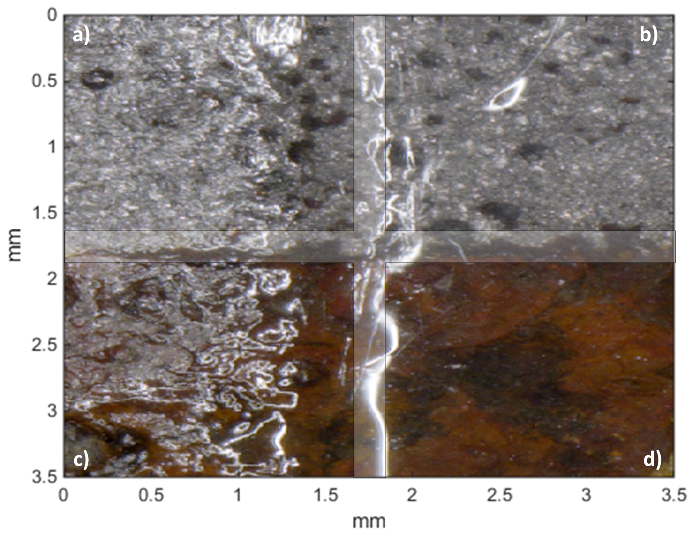
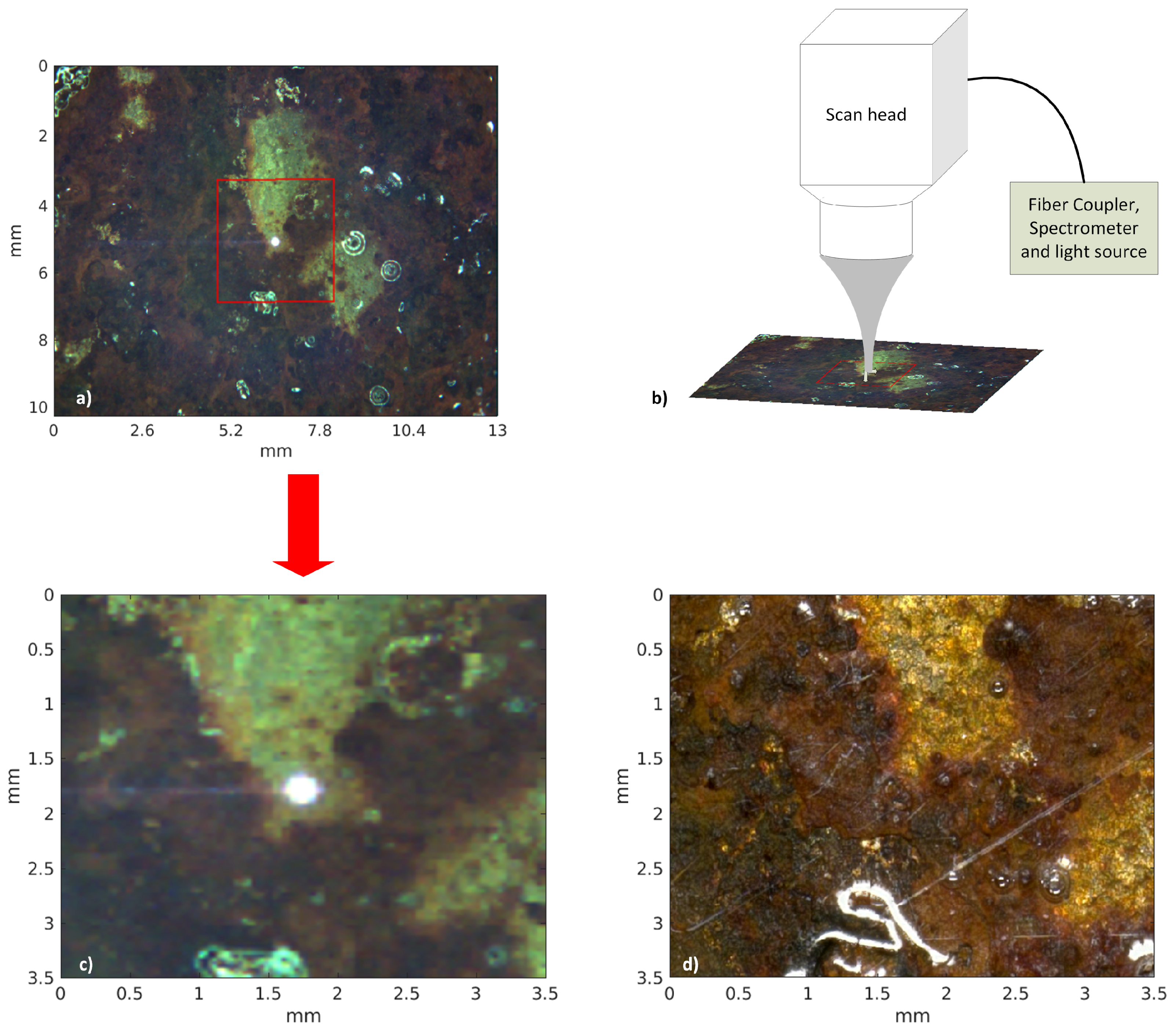
2.2.2. Customized Sectioned Sample

After the different coating layer thicknesses were measured, we created a customized sample which was divided into four regions containing metal and corroded metal with and without a protective coating layer (sample 7, Figure 2).
In order to prepare the desired sample, we first corroded the complete sample artificially by embedding the metal into a natrium chloride bath and exposing it in a climatic chamber afterwards. In more detail, the sample was created following the procedure described in [36]:
  • Embedding in a 5% NaCl-solution
  • Exposure to 100% relative humidity for 8 h at 40 C
  • Drying for 16 h at room temperature
  • Repetition of steps 1 to 3 five times
  • Exposure to outdoor weathering for 2 months inclination 45 , south-side exposure
  • Desalination by immersion with distilled water
  • Soft air abrasive cleaning with walnut shells (pressure 8 bar, distance 50 cm)
  • Additional air abrasive cleaning for half of the sample (upper part) until bare metal was reached.
  • Application of coatings by brush, five to six repetitions (resulting layers), intermediate drying period of 3–4 h for each layer.
To avoid infiltration of the coating, a sellotape stripe was glued before applying the Paraloid B48N onto the sample. However, even by the use of a sellotape stripe, some infiltration zone could be observed.

2.2.3. Standard Sample

Finally, we also prepared a standard sample as is typically used for EIS (sample 8). In contrast to the customized sectioned sample, no defined region for metal or corrosion was present. The preparation was done as described in Section 2.2.2, but without additional air abrasive cleaning (step 8). Furthermore, the complete sample was covered with Paraloid B48N.

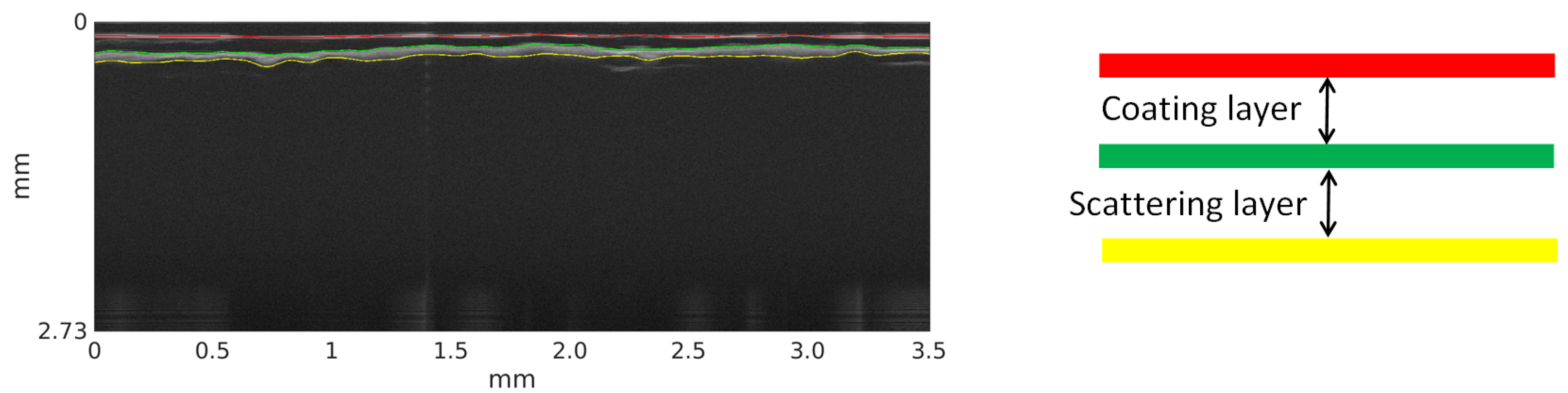
2.3. Post-Processing

Post-processing of the OCT data was done using Matlab (version 2015a, MathWorks, Natick, MA, USA). By utilizing the peak find function in Matlab, several peaks in the OCT A-Scans (line scans perpendicular to the surface) were detected. By choosing optimized parameters and adding appropriate constraints (e.g., thresholding), only the three peaks of interest were determined. The minimum peak prominence and the minimum peak height were the parameters that were optimized.
Using a smoothing algorithm, outliers from the peak detection could be suppressed. Phantom layers caused by autocorrelation were not detected by optimizing the algorithm in terms of intensity. The three peaks of interest correspond to the beginning of the coating layer, the end of the coating layer, and the end of the scattering layer (metal or corrosion). Composing OCT A-Scans along a line parallel to the surface provides a so called B-Scan. A typical B-Scan containing a coating and a scattering layer is shown in Figure 3. Assuming a refractive index of 1.89 for Paraloid B48N, the thickness of the coating layer was calculated by computing the path difference between the second and the first peak and dividing by the refractive index of 1.89. The second layer that was calculated was considered as a scattering layer. Thus, the distance between upper and lower boundary of the material was identified as the scattering layer thickness.

3. Results

3.1. Coated Bare Metal Samples

In Figure 4, the OCT thickness calculations for samples 1–6 are compared to the thickness measurements using the MI system. The mean value for a three-dimensional OCT data set and an error bar using the standard deviation were plotted. The value of the MI system is an average over 50 sampling points that were chosen manually, trying to be as close as possible to the center of the circle. These values and their standard deviation can also be seen for comparison in Table 1.
For thin coating layers, the results of both techniques are in very good agreement with each other. For thicker layers, the values differ. This is due to the fact that the layer had to be brushed or sprayed multiple times for thicker samples. This leads to much more pronounced height variations, as can be seen in Figure 5. As the MI measurements are performed with a hand-held probe, a larger area might be investigated. This might be the reason for a higher standard deviation. Another possibility for the measurement uncertainty could be a density change, leading to a refractive index change as it was previously observed for thicker coatings [13]. For sample S6, increased scattering could be observed, supporting this theory.

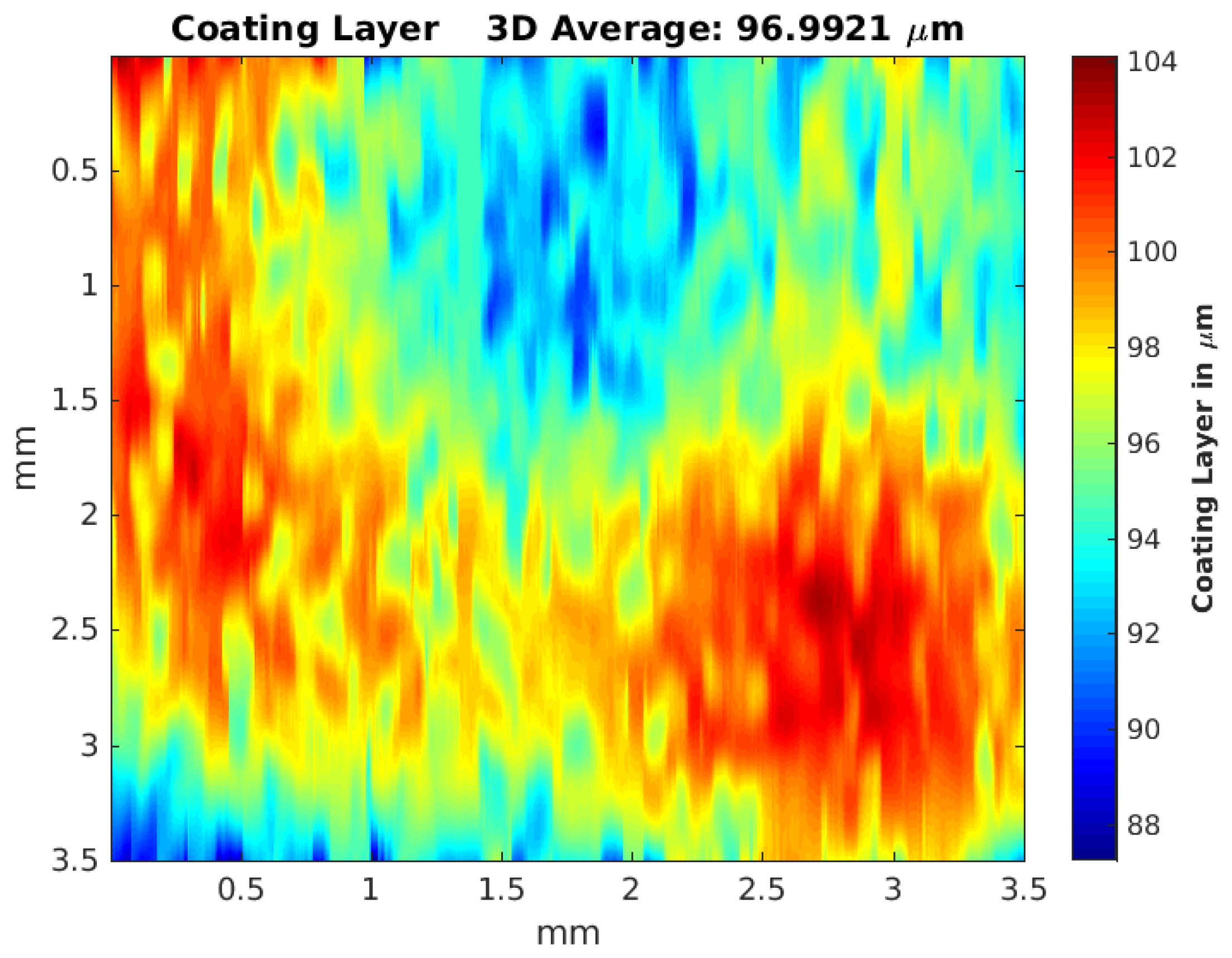
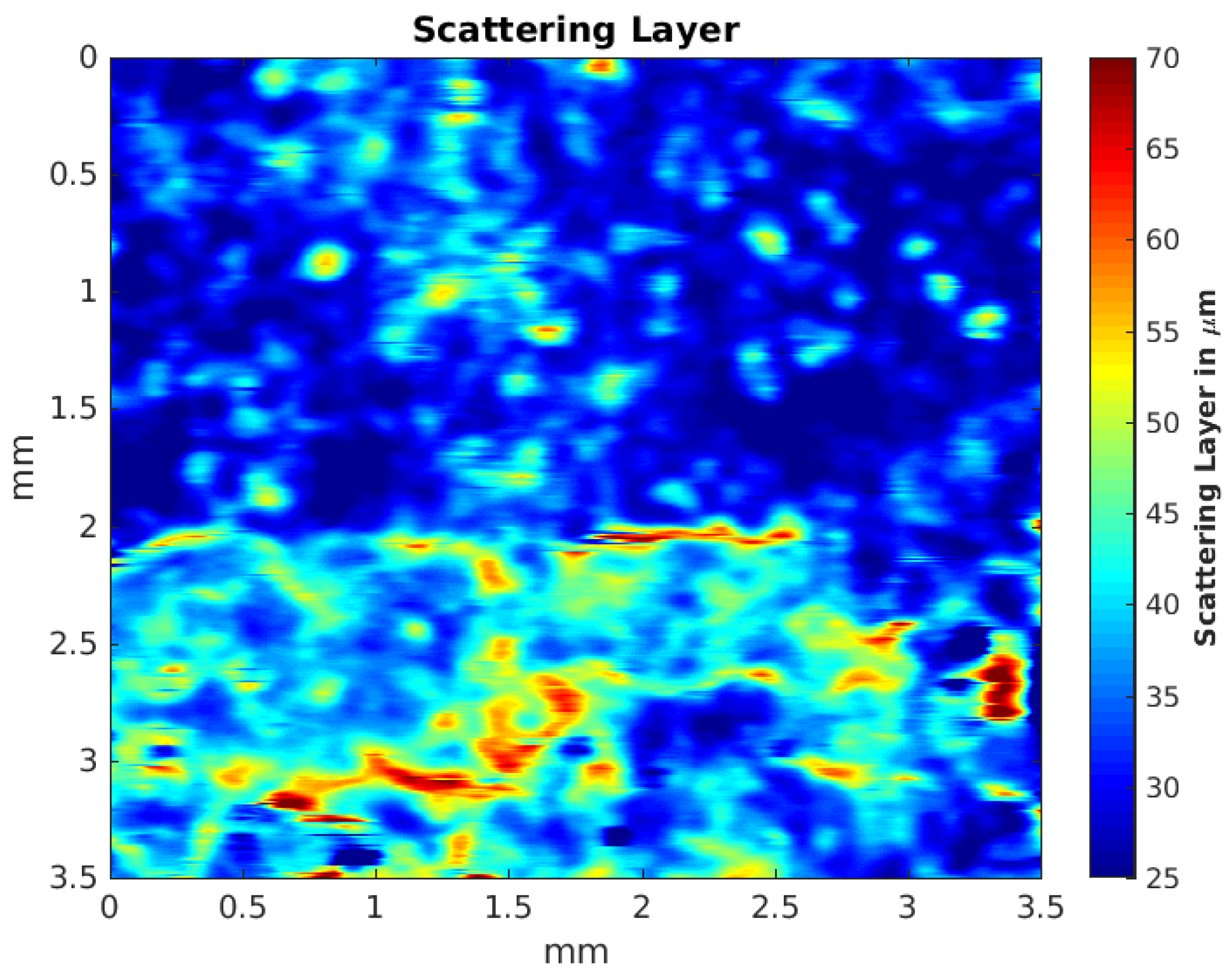
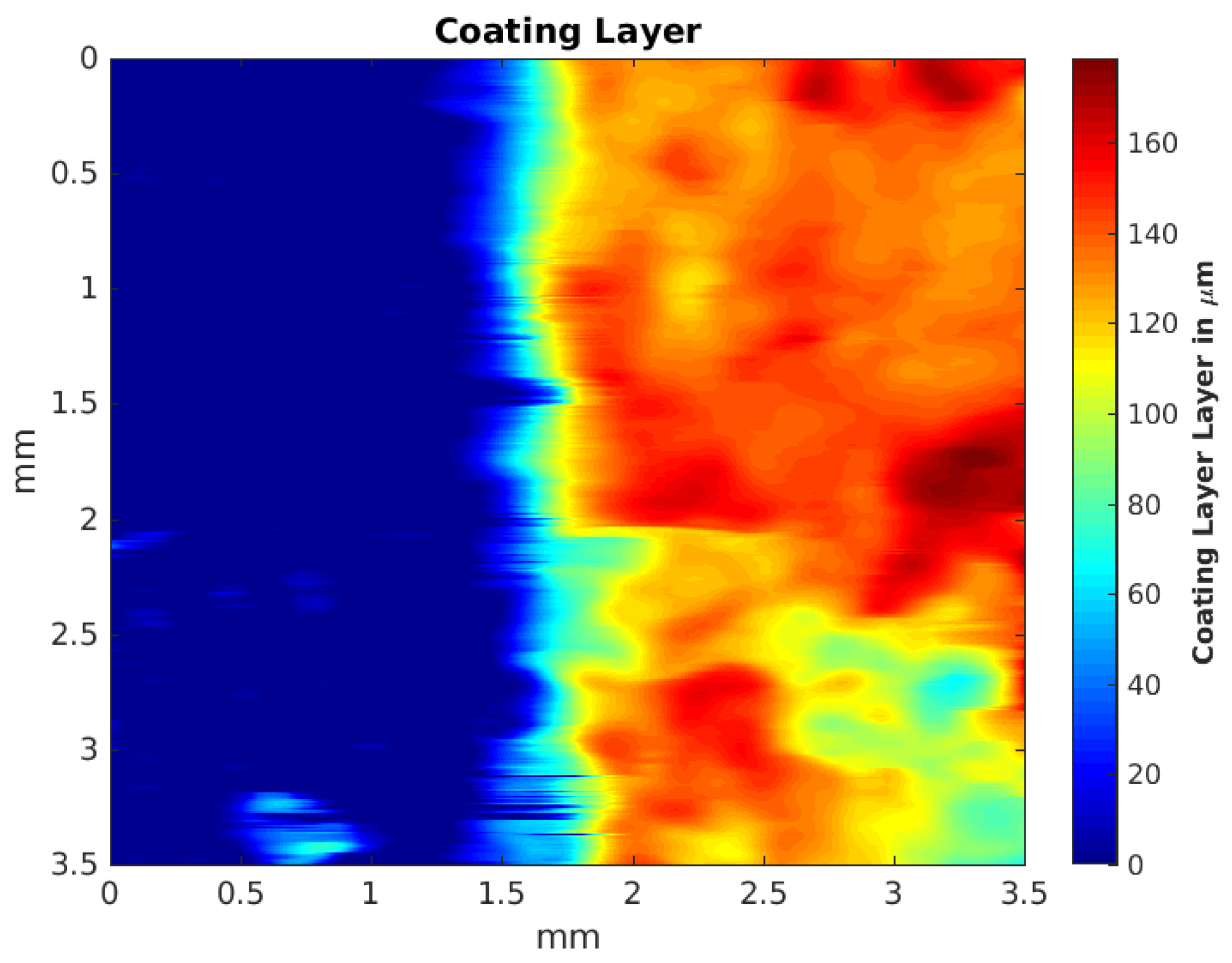
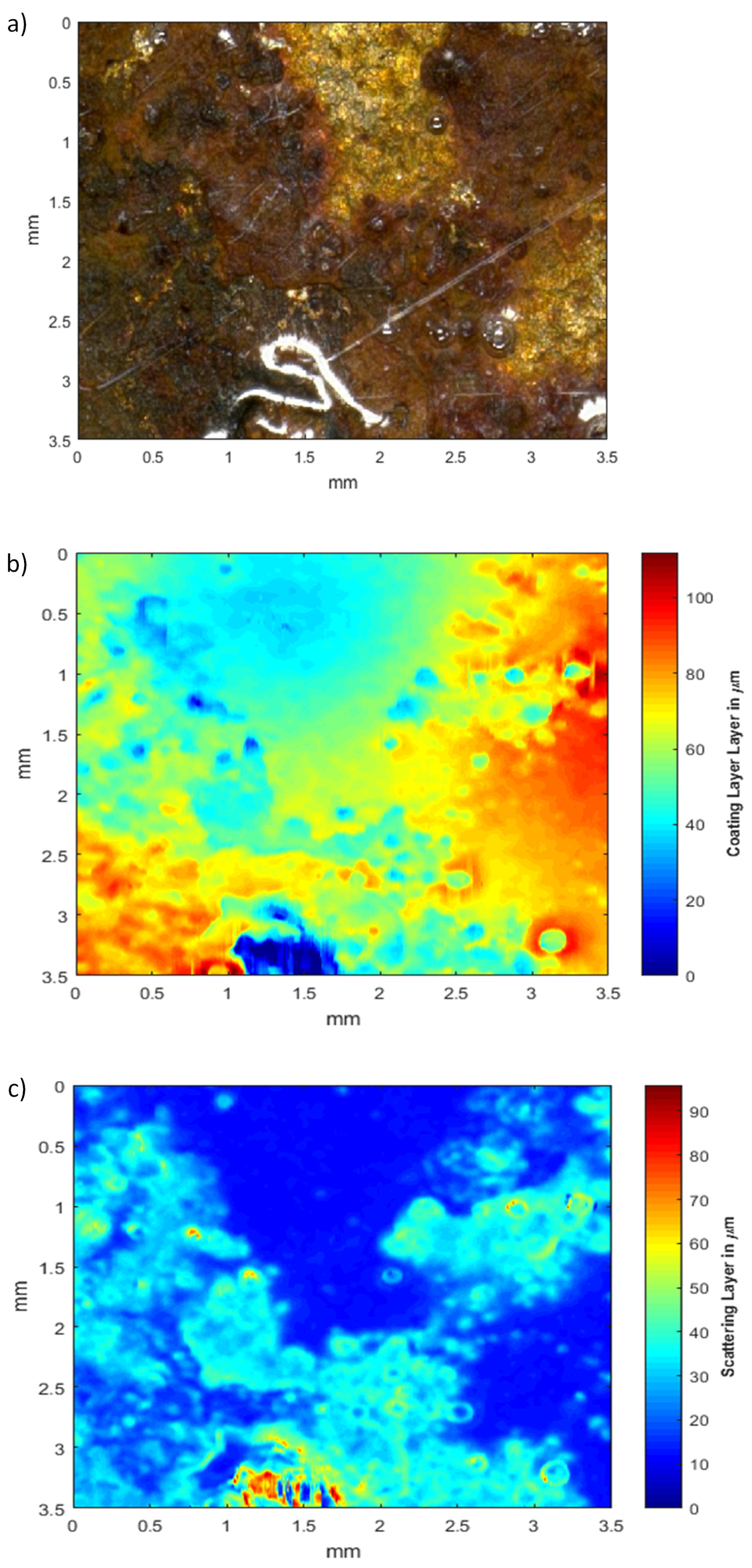
3.2. Customized Sectioned Sample

Figure 6 shows the coating layer thickness for our customized sectioned sample. As could be guessed from the microscopic image in Figure 2, there is no sharp transition from non-coated to protected material.
The transition zone can be clearly identified. Moreover, it can be seen that the coating adheres better on the polished metal than on corrosion, as expected. Our measurements of this sample clearly show that OCT not only provides the layer thicknesses but also enables corroded and non-corroded areas to be clearly distinguised (Figure 7).
The scattering layer thicknesses for the customized sample are shown in Figure 7. For the corroded area, a higher scattering layer thickness can be seen. However, these differences are not as pronounced as in Section 3.3. This is because the complete sample was first corroded artificially. Then, abrasive cleaning was performed to remove the corrosion, but it did not provide a surface as smooth as the initial bare metal. Both findings will be further visualized with measurements on the standard sample in the next subsection.

3.3. Standard Sample

At last, the standard sample described in Section 2.2.3 was investigated with our OCT system. The thickness of the coating and the scattering layer was determined for the complete three-dimensional data set, and a heat map was generated. Figure 8 shows the microscopic image, the coating layer thickness, and the scattering layer thickness. There is a slight shift between the OCT measurement and microscopic image. This is because no additional markers were used in order to prevent any damage to the sample. In Figure 8b, a breach in the coating can be clearly seen (dark blue area). Moreover, Figure 8c shows the difference between pure metal and corroded metal. Pure metal can be recognized as dark blue color. With this sample, we were able to distinguish between metal and corrosion with μ m resolution without a priori knowledge of the distribution of the material. Furthermore, small breaches in the transparent protective coating could be displayed.

4. Discussion

By employing optical coherence tomography as a new powerful tool for the non-destructive testing of metal coatings, additional valuable information about the sample is available. In contrast to electrochemical impedance spectroscopy, OCT provides an imaging modality. Moreover, lateral information about the sample with μ m resolution is available. Further studies with artificial degradation will be performed to evaluate if this lateral resolution is sufficient to estimate the durability of the coatings.
We have proven that the determined thicknesses of the coatings are in good agreement with the theoretically expected values and with the MI measurements. We did not have to change the parameters for different layer thicknesses. However, if a different coating material were to be investigated, these parameters might be adjusted. When analyzing thicker coatings, the standard deviation for the MI measurements tends to rise, but not for the OCT measurements. The differences between the theoretical values and the OCT measurements come from a non-uniform distribution of the material, which cannot be considered at all in the simple theoretical estimation. Another explanation for the uncertainty could be a change in the refractive index, caused by a density change. This deviation appears in particular for thicker samples. Furthermore, a cross-sectional microscopic image would be beneficial to validate our findings. However, the preparation of a cross-sectional sample profile image is difficult to achieve without compromising the sample. During the different preparatory work steps (e.g., cutting, embedding (curing process), and grinding at the end), high temperature can be reached. This is typically destructive for products with low temperature stability, such as Paraloid B48N (glass transition temperature, Tg= 50 C ). Though we have shown that our OCT measurements are already superior to the common MI technique, future applications may induce further demands in terms of axial resolution, field of view, or image acquisition speed:
In our study the thickness of the transparent protective coatings was always more than 6 μ m, so the axial resolution of our OCT system was fully sufficient to differentiate between the different layers. Nevertheless, if thinner coatings would have to be analyzed, OCT systems with 1 μ m axial resolution have already been demonstrated [37].
In our study, we had a field of view of 3.5 × 3.5 mm 2 in which we were able to see the different regions of interest (i.e., corrosion and metal with and without protective coating). However, in future applications, a considerably larger field of view may be required. For that purpose, an OCT system with an enormous field of view in the meter range has been recently reported by Wang et al. [38].
The A-Scan rate of our system was 29 kHz. The time needed to scan an area of 3.5 × 3.5 mm 2 was approximately one minute, which is much faster than an analysis with common EIS systems. However, much less acquisition time may be desired when large objects are investigated. In that case, high-speed OCT systems with scan rates in the MHz range may be used [39].
We are confident that in the future OCT will enable the investigation of real mining objects that have to be conserved, and that all requirements for that purpose will be covered.

5. Conclusions

In this paper, we have demonstrated the benefit of employing optical coherence tomography as a new tool for the investigation of transparent protection coatings. Our comparison with a magnetic inductive layer thickness methodology (which is a commonly used method) validated that precise thickness measurements with OCT are possible, even with underlying corrosion layers. To our knowledge, no other non-destructive modality has provided comparable information. Moreover, by using OCT, the differentiation between metal and corroded material becomes possible with μ m resolution in the lateral dimension. In the future we will perform long-term observations of metal samples with OCT and EIS in order to create additional knowledge in the field of protective layer coatings for preserving cultural heritage in the future. After this first proof of principle, we further want to evaluate the quality of different coatings in terms of performance and long-term stability.

Acknowledgments

This work was financially supported by the Stiftung Rheinisch-Westfälischer Technischer Überwachungsverein (RWTÜV, Essen, Germany) (Project Numbers: S189/10024/2015, S189/10025/2015). We acknowledge support by the the DFG Open Access Publication Funds of the Ruhr-Universität Bochum (Bochum, Germany).

Author Contributions

Marcel Lenz performed the OCT measurements, analyzed the data and wrote the paper. Cristian Mazzon prepared the samples and did the MI measurements. Christopher Dillmann worked on the OCT analysis. Nils C. Gerhardt and Hubert Welp supervised the OCT work and the OCT analysis. Michael Prange supervised the sample preparation and MI measurements and revised the manuscript. Martin R. Hofmann supervised the complete work and edited the manuscript.

Conflicts of Interest

The authors declare no conflict of interest.

References

  1. Hee, M.R.; Izatt, J.A.; Swanson, E.A.; Huang, D.; Schuman, J.S.; Lin, C.P.; Puliafito, C.A.; Fujimoto, J.G. Optical coherence tomography of the human retina. Arch. Ophthalmol. 1995, 113, 325–332. [Google Scholar] [CrossRef] [PubMed]
  2. Welzel, J.; Lankenau, E.; Birngruber, R.; Engelhardt, R. Optical coherence tomography of the human skin. J. Am. Acad. Dermatol. 1997, 37, 958–963. [Google Scholar] [CrossRef]
  3. Drexler, W.; Fujimoto, J.G. Optical Coherence Tomography: Technology and Applications; Springer Science & Business Media: Berlin/Heidelberg, Germany, 2008. [Google Scholar]
  4. Rouba, B.; Karaszkiewicz, P.; Tymioska-Widmer, L.; Iwanicka, M.; Góra, M.; Kwiatkowska, E.; Targowski, P. Optical coherence tomography for non-destructive investigations of structure of objects of art. J. Nondestruct. Test. 2008, 13. [Google Scholar] [CrossRef]
  5. Targowski, P.; Iwanicka, M.; Tymioska-Widmer, L.; Sylwestrzak, M.; Kwiatkowska, E.A. Structural examination of easel paintings with optical coherence tomography. Acc. Chem. Res. 2009, 43, 826–836. [Google Scholar] [CrossRef] [PubMed]
  6. Targowski, P.; Iwanicka, M. Optical coherence tomography: Its role in the non-invasive structural examination and conservation of cultural heritage objects—A review. Appl. Phys. A 2012, 106, 265–277. [Google Scholar] [CrossRef]
  7. Wiesauer, K.; Pircher, M.; Götzinger, E.; Hitzenberger, C.K.; Oster, R.; Stifter, D. Investigation of glass–fibre reinforced polymers by polarisation-sensitive, ultra-high resolution optical coherence tomography: Internal structures, defects and stress. Compos. Sci. Technol. 2007, 67, 3051–3058. [Google Scholar] [CrossRef]
  8. Stifter, D.; Wiesauer, K.; Wurm, M.; Schlotthauer, E.; Kastner, J.; Pircher, M.; Götzinger, E.; Hitzenberger, C. Investigation of polymer and polymer/fibre composite materials with optical coherence tomography. Measur. Sci. Technol. 2008, 19, 074011. [Google Scholar] [CrossRef]
  9. Duncan, M.D.; Bashkansky, M.; Reintjes, J. Subsurface defect detection in materials using optical coherence tomography. Opt. Express 1998, 2, 540–545. [Google Scholar] [CrossRef] [PubMed]
  10. Stifter, D.; Burgholzer, P.; Höglinger, O.; Götzinger, E.; Hitzenberger, C.K. Polarisation-sensitive optical coherence tomography for material characterisation and strain-field mapping. Appl. Phys. A 2003, 76, 947–951. [Google Scholar] [CrossRef]
  11. Wiesauer, K.; Pircher, M.; Götzinger, E.; Bauer, S.; Engelke, R.; Ahrens, G.; Grützner, G.; Hitzenberger, C.; Stifter, D. En-face scanning optical coherence tomography with ultra-high resolution for material investigation. Opt. Express 2005, 13, 1015–1024. [Google Scholar] [CrossRef] [PubMed]
  12. Zhong, S.; Shen, Y.C.; Ho, L.; May, R.K.; Zeitler, J.A.; Evans, M.; Taday, P.F.; Pepper, M.; Rades, T.; Gordon, K.C.; et al. Non-destructive quantification of pharmaceutical tablet coatings using terahertz pulsed imaging and optical coherence tomography. Opt. Lasers Eng. 2011, 49, 361–365. [Google Scholar] [CrossRef]
  13. Lin, H.; Dong, Y.; Shen, Y.; Zeitler, J.A. Quantifying pharmaceutical film coating with optical coherence tomography and terahertz pulsed imaging: An evaluation. J. Pharm. Sci. 2015, 104, 3377–3385. [Google Scholar] [CrossRef] [PubMed]
  14. Serrels, K.A.; Renner, M.K.; Reid, D.T. Optical coherence tomography for non-destructive investigation of silicon integrated-circuits. Microelectron. Eng. 2010, 87, 1785–1791. [Google Scholar] [CrossRef]
  15. Stifter, D. Beyond biomedicine: A review of alternative applications and developments for optical coherence tomography. Appl. Phys. B 2007, 88, 337–357. [Google Scholar] [CrossRef]
  16. Nemeth, A.; Leiss-Holzinger, E.; Hannesschläger, G.; Wiesauer, K.; Leitner, M. Optical Coherence Tomography- Applications in Non-Destructive Testing and Evaluation; INTECH Open Access Publisher: Rijeka, Croatia, 2013. [Google Scholar]
  17. Mazzon, C.; Letardi, P.; Brüggerhoff, S. Development of Monitoring Techniques for Coatings Applied to Industrial Heritage. In Proceedings of the BigStuff 2015–Technical Heritage: Preserving Authenticity-Enabling Identity, Lewarde, France, 3–4 September 2015. [Google Scholar]
  18. Mansfeld, F. Electrochemical impedance spectroscopy (EIS) as a new tool for investigating methods of corrosion protection. Electrochim. Acta 1990, 35, 1533–1544. [Google Scholar] [CrossRef]
  19. Letardi, P.; Spiniello, R. Characterisation of Bronze Corrosion and Protection by Contact-Probe Electrochemical Impedance Measurements. In Proceedings of the Metal 2001: Proceedings of the International Conference on Metals Conservation, Santiago, Chile, 2–6 April 2001; Western Australian Museum: Fremental, Australia, 2004; pp. 316–319. [Google Scholar]
  20. Mottner, P. Investigations of Transparent Coatings for the Conservation of Iron and Steel Outdoor Industrial Monuments. In Proceedings of the Metal 2001: Proceedings of the International Conference on Metals Conservation, Santiago, Chile, 2–6 April 2001; Western Australian Museum: Fremental, Australia, 2004; pp. 279–288. [Google Scholar]
  21. Angelini, E.P.M.V.; Assante, D.; Grassini, S.; Parvis, M. EIS measurements for the assessment of the conservation state of metallic works of art. Int. J. Circuits Syst. Signal Process. 2014, 8, 240–245. [Google Scholar]
  22. Cano, E.; Crespo, A.; Lafuente, D.; Barat, B.R. A novel gel polymer electrolyte cell for in-situ application of corrosion electrochemical techniques. Electrochem. Commun. 2014, 41, 16–19. [Google Scholar] [CrossRef]
  23. Cano, E.; Lafuente, D.; Bastidas, D.M. Use of EIS for the evaluation of the protective properties of coatings for metallic cultural heritage: A review. J. Solid State Electrochem. 2010, 14, 381–391. [Google Scholar] [CrossRef]
  24. Ellingson, L.A.; Shedlosky, T.J.; Bierwagen, G.P.; de la Rie, E.R.; Brostoff, L. The use of electrochemical impedance spectroscopy in the evaluation of coatings for outdoor bronze. Stud. Conserv. 2013, 49, 53–62. [Google Scholar] [CrossRef]
  25. Hallam, D.; Thurrowgood, D.; Otieno-Alego, V.; Creagh, D. An EIS Method for Assessing Thin Oil Films Used in Museums. In Proceedings of the Metal 2004 National Museum of Australia Canberra ACT, Canberra, Australia, 4–8 October 2004; Volume 4, p. 8. [Google Scholar]
  26. Letardi, P. Corrosion and Conservation of Cultural Heritage Metallic Artefacts: 7. Electrochemical Measurements in the Conservation of Metallic Heritage Artefacts: An Overview; Elsevier Inc.: Amsterdam, The Netherlands, 2013. [Google Scholar]
  27. Letardi, P.; Beccaria, A.; Marabelli, M.; D’ERCOLI, G. Application of Electrochemical Impedance Measurements as a Tool for the Characterization of the Conservation and Protection State of Bronze Works of Art. In Proceedings of the Conférence Internationale sur la Conservation des Métaux, Draguignan, France, 27–29 May 1998; pp. 303–308. [Google Scholar]
  28. Mansfeld, F. Use of electrochemical impedance spectroscopy for the study of corrosion protection by polymer coatings. J. Appl. Electrochem. 1995, 25, 187–202. [Google Scholar] [CrossRef]
  29. Price, C.; Hallam, D.; Heath, G.; Creagh, D.; Ashton, J. An Electrochemical Study of Waxes for Bronze Sculpture. In Proceedings of the Conférence Internationale sur la Conservation des Métaux, Semur en Auxois, France, 25–28 September 1995; pp. 233–241. [Google Scholar]
  30. Amirudin, A.; Thieny, D. Application of electrochemical impedance spectroscopy to study the degradation of polymer-coated metals. Prog. Org. Coat. 1995, 26, 1–28. [Google Scholar] [CrossRef]
  31. Fischer, H. Electromagnetic Probe for Measuring the Thickness of Thin Coatings on Magnetic Substrates. US Patent 4,829,251, 9 May 1989. [Google Scholar]
  32. Wolfram, J.; Brüggerhoff, S.; Eggert, G. Better Than Paraloid B-72? Testing Poligen Waxes as Coatings for Metal Objects. In Proceedings of the METAL 2010: Proceedings of the Interim Meeting of the ICOM-CC Metal Working Group, Clemson University, Clemson, SC, USA, 11–15 October 2010; pp. 124–131. [Google Scholar]
  33. Antoniuk, P.; Strąkowski, M.; Pluciński, J.; Kosmowski, B. Non-Destructive Inspection of Anti-corrosion protective coatings using optical coherent tomography. Metrol. Measur. Syst. 2012, 19, 365–372. [Google Scholar] [CrossRef]
  34. Derrick, M. Paraloid B-48N. Available online: http://cameo.mfa.org/wiki/ParaloidB-48N (accessed on 16 January 2017).
  35. Decker, P.; Brüggerhoff, S.; Eggert, G. To coat or not to coat? The maintenance of Cor-Ten® sculptures. Mater. Corros. 2008, 59, 239–247. [Google Scholar] [CrossRef]
  36. Seipelt, B.; Pilz, M.; Kiesenberg, J. Transparent Coatings-Suitable Corrosion Protection for Industrial Heritage Made of Iron? In Proceedings of the Conférence Internationale sur la Conservation des Métaux, Draguignan, France, 27–29 May 1998; pp. 291–296. [Google Scholar]
  37. Dubois, A.; Vabre, L.; Boccara, A.C.; Beaurepaire, E. High-resolution full-field optical coherence tomography with a Linnik microscope. Appl. Opt. 2002, 41, 805–812. [Google Scholar] [CrossRef] [PubMed]
  38. Wang, Z.; Potsaid, B.; Chen, L.; Doerr, C.; Lee, H.C.; Nielson, T.; Jayaraman, V.; Cable, A.E.; Swanson, E.; Fujimoto, J.G. Cubic meter volume optical coherence tomography. Optica 2016, 3, 1496–1503. [Google Scholar] [CrossRef] [PubMed]
  39. Klein, T.; Huber, R. High-speed OCT light sources and systems [Invited]. Biomed. Opt. Express 2017, 8, 828–859. [Google Scholar] [CrossRef] [PubMed]
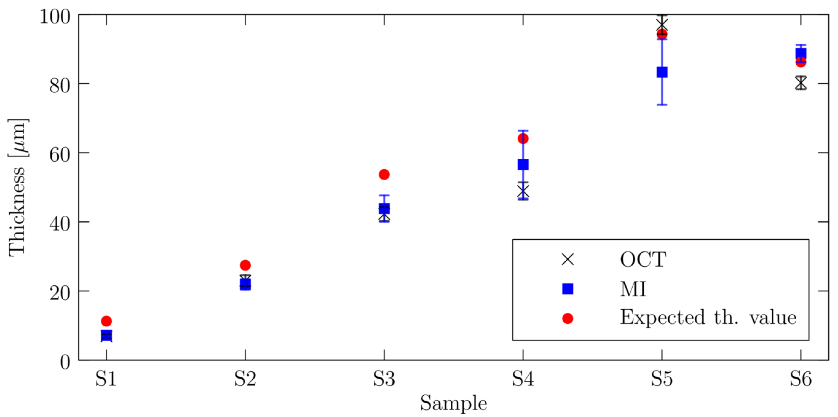
Figure 1. (a) Snapshot taken with the in-built camera of the optical coherence tomography (OCT) system of a standard sample; (b) measurement schematic; (c) interpolated video image; (d) microscopic image of the region of interest.
Applsci 07 00364 g001
Figure 2. Microscopic image of the customized sectioned sample: (a) pure metal; (b) pure metal with coating layer on top; (c) corroded area; (d) corroded material with coating layer on top.
Applsci 07 00364 g002
Figure 3. OCT B-Scan of corroded metal (sample 8): red line is the top of the coating layer, green line determines the end of the coating and the beginning of the corrosion, yellow line determines the end of the scattering-induced layer. Axes are given as optical path length n × d .
Applsci 07 00364 g003
Figure 4. Comparison between OCT and MI measurements and the calculated theoretical value.
Applsci 07 00364 g004
Figure 5. 3D heat map of the calculated layer thickness for the OCT measurement of sample 5.
Applsci 07 00364 g005
Figure 6. 3D heat map of the calculated coating layer thickness for the OCT measurement of the customized sample (sample 7).
Applsci 07 00364 g006
Figure 7. 3D heat map of the calculated scattering layer thickness for the OCT measurement of the customized sample (sample 7).
Applsci 07 00364 g007
Figure 8. (a) Microscopy image of a standard sample (sample 8); (b) heat map of the calculated layer thickness for the OCT measurement; (c) heat map of the calculated scattering layer thickness for the OCT measurement.
Applsci 07 00364 g008
Table 1. Comparison between optical coherence tomography measurement, magnetic inductive (MI) measurement, and the expected theoretical values. The sprayed sample is marked with an *. All thickness values are given in μ m.
ConceptSample 1Sample 2Sample 3Sample 4Sample 5Sample 6 *
OCT6.8622.9742.2748.9197.0080.24
std. OCT0.651.612.012.522.741.85
MI7.1621.8943.8556.5783.3488.70
std. MI1.141.53.89.819.472.5
expected th. value11.2727.4453.7064.1094.3086.26

