Vehicle Loads for Assessing the Required Load Capacity Considering the Traffic Environment


1
School of Civil & Environmental Engineering, Yonsei University, Seoul 03722, Korea
2
Smart Facilities Management Division, Korea Infrastructure, Safety and Technology Corporation, Jinju 52852, Korea
*
Author to whom correspondence should be addressed.
Appl. Sci. 2017, 7(4), 365; https://doi.org/10.3390/app7040365
Submission received: 1 December 2016
/
Revised: 4 April 2017
/
Accepted: 5 April 2017
/
Published: 6 April 2017
Abstract
:The effects of traffic loads on existing bridges are quite different from those of design live loads because of the various traffic environments. However, the bridge maintenance and safety assessment of in-service bridges maintain the design load capacity without considering the current traffic environment. The real traffic conditions on existing bridges may require a load capacity that is considerably different from the design. Therefore, the required load capacity of an existing highway bridge should be determined according to the extreme load effects that the bridge will experience from the actual traffic environment during its remaining service life for more rational maintenance of the infrastructure. A simulation process was developed to determine evaluation vehicle loads for bridge safety assessment based on the extreme load effects that may occur during the remaining service life. Realistic probabilistic traffic models were used to reflect the actual traffic environment. The presented model was used to analyze the extreme load effect on pre-stressed concrete (PSC) and steel box girder bridges, which are typical bridge types. The traffic environmental conditions included the traffic volume (2000–40,000), the proportion of heavy vehicles (15–45%), and the consecutive vehicle traveling patterns. The spans of the sample bridges were 30 m (PSC bridge) and 45 or 60 m (steel box girder bridge). In the results, the extreme load effects tended to increase with either the traffic volume or proportion of heavy vehicles. The evaluation vehicle loads for bridge safety assessment may be adjusted with the traffic conditions, such as the traffic volume, the proportion of heavy vehicles, and the consecutive vehicle traveling patterns.
1. Introduction
Current bridge design is based on conservative assumptions regarding the intensity of applied loads and the structural response of a bridge to these loads. Although these designs have served the public very well by providing a network of safe and economical bridge infrastructure systems, they may not offer the most optimum approach to assessing the safety of existing bridges. Due to the nominal reduction in the required load capacities of bridges that have been in service for many years, using the design criteria to assess their safety may indicate that many of them need upgrading. However, the direct and user costs associated with upgrading a single existing bridge are generally quite high, and the costs of upgrading a network of bridges are prohibitive. Therefore, some of the conservatism that is normally incorporated into the design requirements for new bridges and in-service bridges needs to be revisited and, if possible, reduced when assessing the required performance of existing bridges [1].
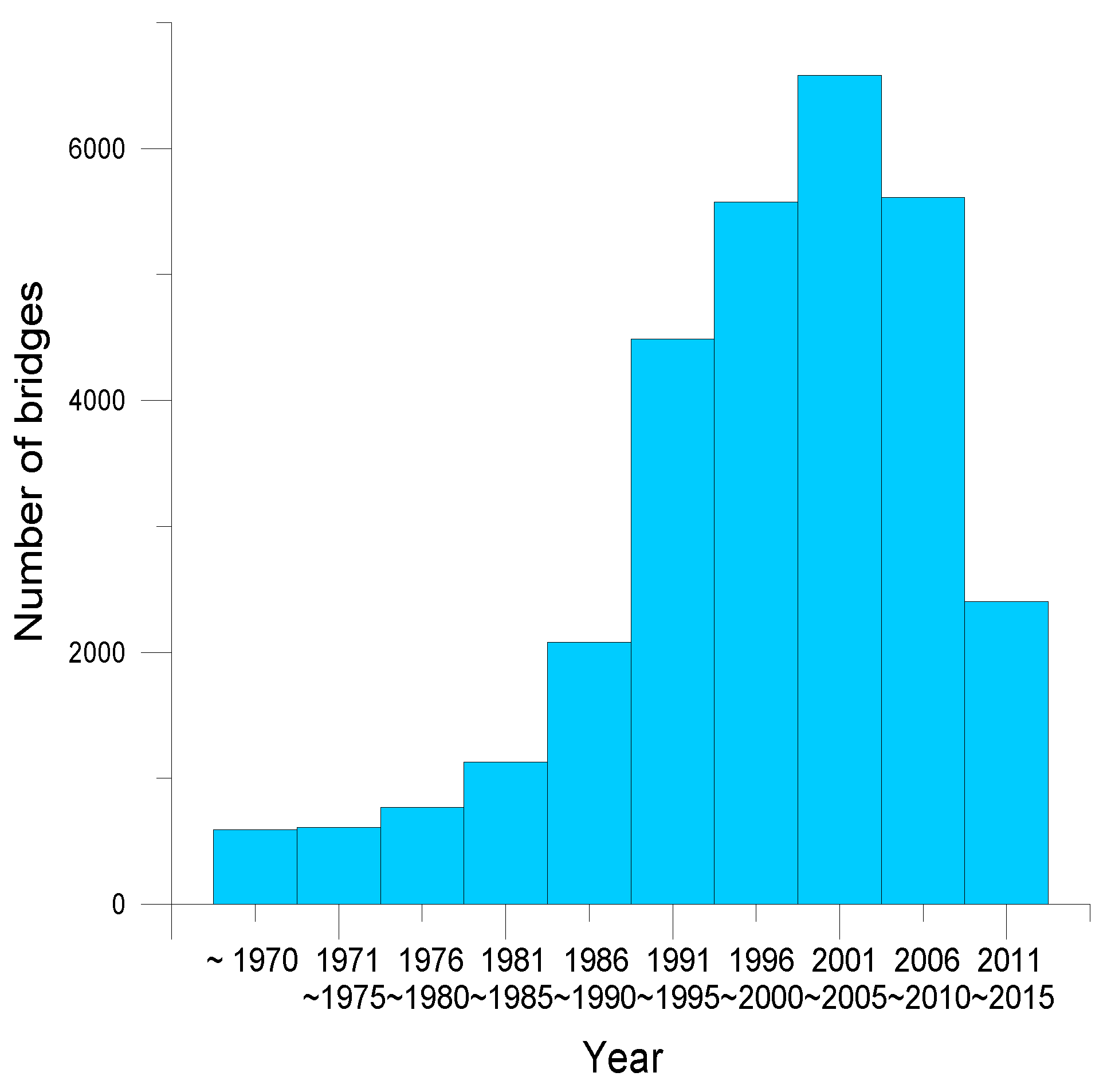
There are approximately 29,896 bridges currently in service in Korea as of 2014. Figure 1 shows the number of bridges according to the year of construction completion. According to the data, the number of newly-built bridges rapidly increased in the 1990s, and the highest number of new bridges was built in the 2000s. However, the number of newly-built bridges has been decreasing rapidly since 2010. Bridges were built in the 1990s to satisfy the demand for infrastructure from active social development, but the number of newly-built bridges has been decreasing since the 2000s because of the expansion of previously planned infrastructure [2].
Recently, extreme vehicle loads have been researched through methods such as the distribution model and simulation. González et al. [3] analyzed the critical load scenarios determined from a Monte Carlo simulation. Gu et al. [4] presented a Bayesian distribution model of overloaded vehicles. O’Brien et al. developed traffic load models with various probabilistic methods [5,6,7,8]. They also considered the dynamic effects in addition to static effects [9]. The required performance of a bridge structure may vary depending on the expected user level [10]. The effects of the traffic load on existing bridges are quite different from those of live design loads owing to the various traffic environments. However, the bridge maintenance and safety assessment of in-service bridges focus on maintaining the required load capacities that were determined in the design stage without considering the actual traffic environment. The real traffic conditions on existing bridges may require load capacities that are considerably different, either higher or lower, from the design load capacity. Therefore, the target required load capacity of an existing highway bridge should be determined according to the extreme load effects that the bridge will experience in the actual traffic environment during its remaining service life to provide a more rational and economical maintenance of the infrastructure.
This paper presents a simple traffic model for estimating probabilities as a function of the traffic environment and proposes a rational maintenance procedure to determine the required load capacities of existing bridges by evaluating the required performance based on actual road traffic conditions. The aim is to achieve consistent safety levels for existing bridges through proper maintenance, even under quite different traffic load conditions, such as different traffic volumes (average daily traffic, ADT) and heavy vehicle volumes (average daily truck traffic, ADTT). According to the proposed procedure, probabilistic vehicle weight models and consecutive traveling vehicle models are suggested based on the field data. In addition, traveling speed proportion models and headway models are proposed, as well as heavy vehicle distribution models for lanes on multi-lane roads.
2. Concept of Probability-Based Assessment and Target Performance Levels
Among bridges currently in service, first-class bridges are designed by considering the target performance of the current design load: the DB24 truck loading of the Korea Institute of Bridge and Structural Engineers (KIBSE). A DB24 truckload is approximately 1.3 times heavier than the HS20 truckload specified in AASHTO LRFD [11]. However, bridges in actual service tend to experience higher or lower load effects than the existing target performance depending on the traffic volume in the relevant area or traffic characteristics of heavy and consecutive vehicles. Current performance evaluation and maintenance of bridges secure a uniform performance level according to the target performance determined in the design phase. In some cases, therefore, budgets are allocated to secure a superior level of bridge performance than required, which indicates a general lack of rationality in bridge maintenance.
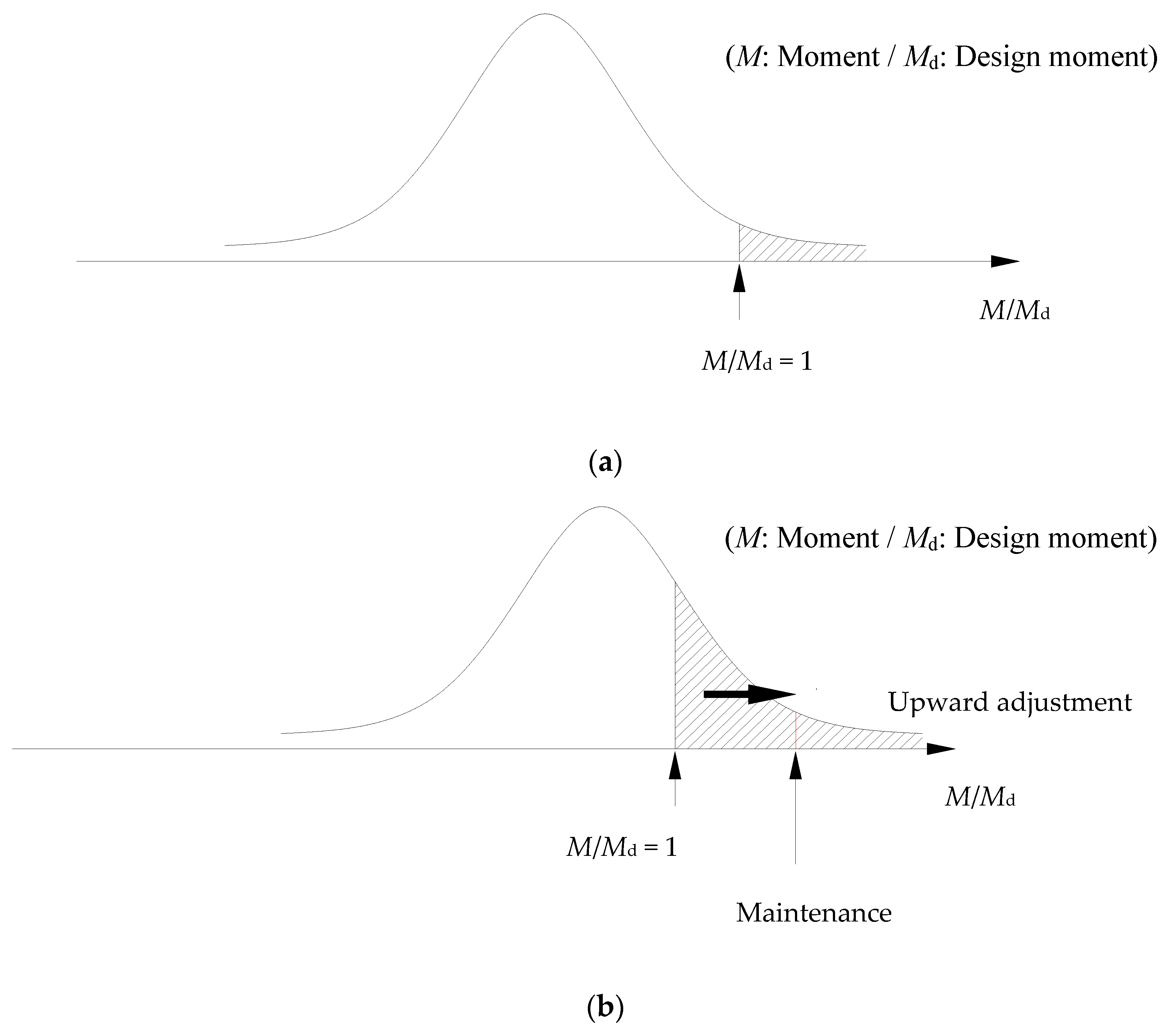
For example, Figure 2a shows the probability distribution of the load effect experienced by a representative bridge with a traffic environment equivalent to the national average. The hatched areas represent the probability that the design load effect (Md) will be exceeded. However, if there is an above-average traffic volume or the area has a high proportion of heavy vehicles (Figure 2b, the experienced load effect increases, and there is a greater probability that the design load effect will be exceeded. In areas with a low traffic volume or heavy vehicle proportion (Figure 2c), there is a lower probability that the design load effect will be exceeded. Therefore, the efficiency of the current evaluation and maintenance of bridges can be increased by adequately adjusting the required performance standard. In other words, adjusting the control level upward (Figure 2b) or downward (Figure 2c) can maintain the probability that the required performance will be exceeded by the traffic vehicle load at a consistent level. This will also add consistency to damage progression and deterioration of a target bridge structure from the vehicle load due to the site environment. The efficient distribution of bridge maintenance costs can also be realized by using this rational approach to the required performance. Since the budget for road and bridge maintenance is expected to exceed 40% after 2020 [12], it seems necessary to improve current uniform bridge maintenance policies based on the target performance of the design phase.
Based on this perspective, the required performance considering the traffic environments was analyzed by considering the extreme load effect that may occur on a bridge reflecting the regional traffic environment and structural characteristics, such as the average daily traffic volume, heavy vehicle proportion, heavy vehicle traffic rate per lane, and girder type.
3. Probabilistic Vehicle Models of Weights and Traveling Patterns
The loads that constantly occur on highway bridges as a result of passing vehicles are generally reflected by the design live load. Thus, a load that influences the safety of a highway bridge is much higher with a relatively low frequency. Vehicle loads can generally be divided into cases with a single overloaded heavy vehicle or with consecutive vehicles. However, because a single heavy vehicle has a limited loading capacity, the consecutive traffic of heavy vehicles is classified as a higher risk.
The risk associated with consecutive heavy vehicles increases when the headway is narrow during traffic congestion with an extremely low travel speed, which increases the number of vehicles on the highway bridge. Moreover, for consecutive vehicles, there is a high frequency of certain vehicle types (particularly heavy vehicles) depending on the driving or passing ability of the vehicle. The safety of highway bridges is most affected by heavy vehicles traveling consecutively at a low speed, as shown in Figure 3.
3.1. Classification of Vehicles
To determine the extreme load effects of bridges, the maximum live load needs to be analyzed by considering the probabilistic model of traveling vehicles. This section provides supplementary data for modeling traveling vehicles and assumptions for extreme load effect analysis.
Overweight vehicles can be increasingly found on roads because of developments in the car industry. In this study, five representative vehicle models were selected among the vehicle classifications of the Korean Ministry of Land, Transport, and Maritime Affairs [13]: P, B, T, TT, and ST representing a mobile car, bus, small-sized truck, mid-sized truck, and heavy truck, respectively. Table 1 defines these models. The axle loads of each model were assumed to be concentrated loads. Table 2 gives the load distributions and dimensions for each model.
3.2. Proposed Vehicle Weight Models
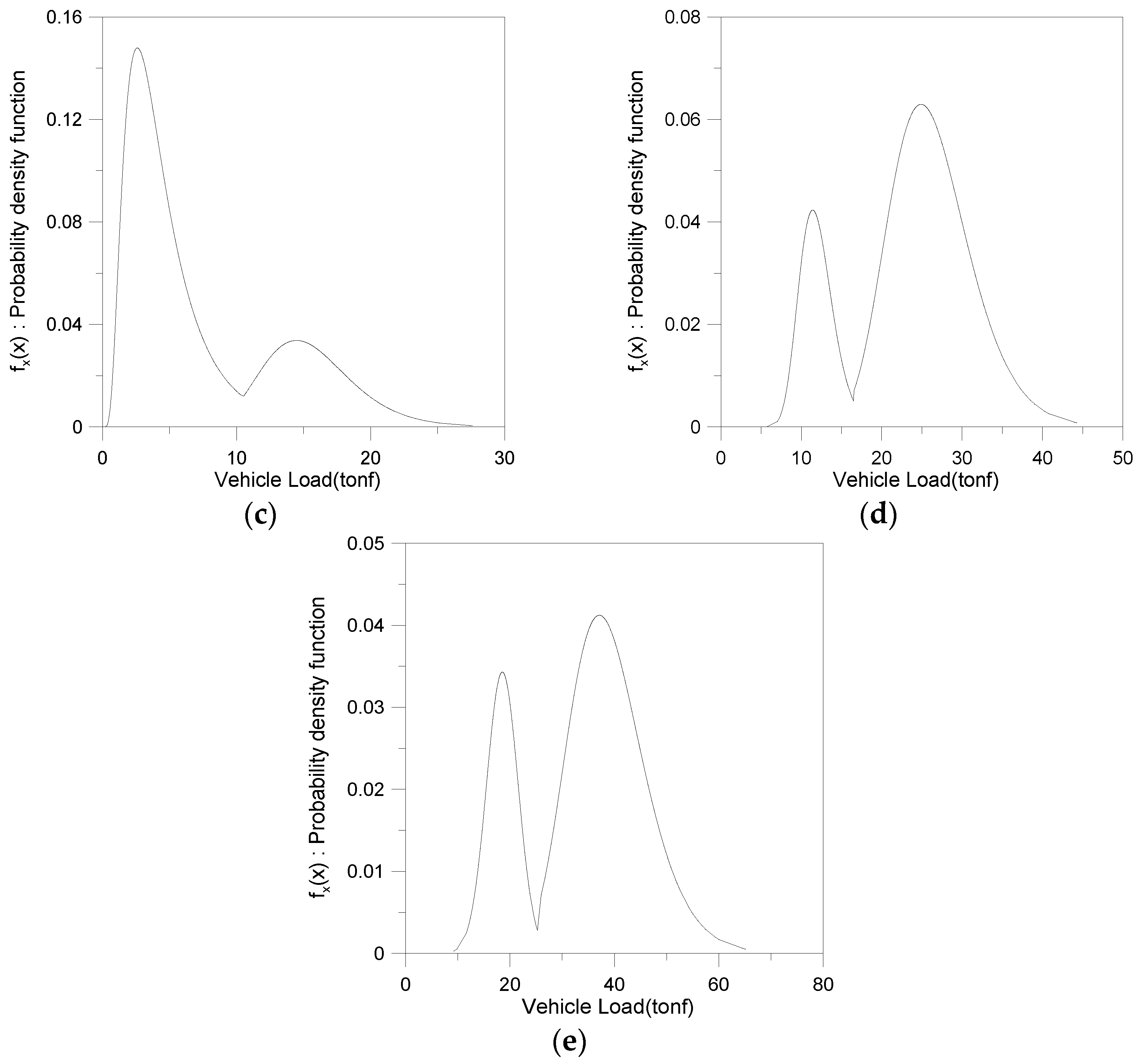
Table 3 lists the total weight distribution characteristics of the five representative vehicle models based on an analysis of the collected data on the probabilistic characteristics of loads in a previous study [14]. The P type (i.e., mobile car) has a complete unimodal distribution, while the other types show a bimodal distribution, which agrees with data from a previous investigation [15]. This characteristic was clearly displayed in large heavy vehicles such as the TT and ST types. The first mode for the vehicle weight distribution of each model generally reflects empty or partially-loaded vehicles or light cargo carriers, and the second mode reflects vehicles with a full load. The third mode models the top 1% portion of the second model to show the characteristics of an overloaded vehicle.
For Korean highway bridges, the vehicle weight is limited to less than 40 tons. The proposed model and actual weigh-in-motion (WIM) data were compared to verify the proposed model. The WIM data was recorded on Jungbu-Naeryuk highway in Korea [16]. There were 61,090 total vehicles and 705 overloaded vehicles. The proportion of overloaded vehicles was estimated to be 1.2%. The proposed model estimated the overloaded vehicle proportion to be 1.9%. Since bridge design is conservative, the proposed vehicle weight model seems to perform well.
Table 4 presents the current status (from January 2011 to June 2013) of overloaded vehicle control according to the National Road Management Offices in Korea. The population size was estimated by using data from 5033 cases of overloaded vehicles that exceeded the total weight standard in seven regions.
A field survey was performed to develop the probabilistic load models for each type of vehicle, as given in Table 5 and Figure 4. The field survey was performed simultaneously on national highways (Regions I–VII) in Korea, which have vehicle load weighing machines. The indices and are the average and standard deviation, respectively, for a normal distribution. The indices and represent the average and standard deviation, respectively, for a log-normal distribution. The first mode indicates the empty or lightly-loaded condition, and the second mode represents the heavily-loaded condition. The minimum values in Table 5 indicate the minimum weights of the vehicle model, while the maximum values indicate the summation of maximum loads on each vehicle axle. Correction coefficients were used to calibrate the distribution curve by considering the maximum and minimum values as a ratio of each mode. For the purpose of simplification, multiple tandems in each vehicle model were modeled as a single tandem (i.e., P, B, T, and TT were modeled as two-axle vehicles, and ST has three axles).
3.3. Traffic Flow Characteristics
Traveling patterns of vehicles vary according to the speed and daily traffic volume. In addition, headway distances between vehicles should be determined rationally to model the traveling vehicles. Table 6 presents the results of the field survey at five points on Korean national highways [17]. The locations of the field survey were selected according to the exceedance of the average heavy vehicle proportion and traffic volume. The survey considered peak times. The traffic volumes at the five locations were 3056, 4396, 3976, 3409, and 7814. To analyze the traffic characteristics of vehicles traveling over bridges, an observation location was selected on a representative national road to consider the hourly traffic volume, influence of the commuting time, and driving hours of heavy vehicles.
Based on the field survey, the proportion and mean headway distance were determined for each vehicle speed, as given in Table 7. When the vehicle speed was above 50 km/h, then the headway distance was set to 25 m. This is because larger headway distances would have a weak effect on the bridge.
3.4. Probabilistic Consecutive Models of Traveling Vehicles
The consecutive vehicle model in this study was previously developed in [14]. The probabilistic matrix, which represents consecutive vehicles, can be determined from traffic data analyzed from national roads in Korea. By using the vehicle models presented in the previous section, the matrix can be written as:
where is the probability of the vehicle type j following the vehicle type i. The probability of n vehicles of the vehicle type m running consecutively is:
where is the simple traffic composition rate of the vehicle type m.
Table 8 lists the consecutive traveling coefficients and proportions of single vehicles to heavy vehicles. The heavy vehicle proportions of 15%, 25%, 35%, and 45% were established as basic proportions. A consecutive traveling probability equivalent to 15% was applied to areas with a proportion of 15% and below, whereas that equivalent to 45% was applied to areas with a proportion of 45% and above. In areas with a heavy vehicle proportion ranging from 15% to 45%, the consecutive traveling probability was estimated by assuming that the consecutive traveling coefficient varies linearly between the representative models given in Table 8 according to the basic proportions of heavy vehicles.
4. Evaluation of Extreme Load Effects
4.1. Data Processing for Extreme Load Effect Analysis
A large amount of traffic operates over a bridge during its service life. Predicting the extreme load effect by analytical means is very complicated. Instead of all of the traffic over a bridge being considered, the computational simulations in this study were performed with a unit traffic volume, and the extreme load effect was analyzed by using an extreme value distribution. The extreme load effects from the simulations were modeled as a Gumbel type-I distribution [18,19]. Since the axle load distributions for all vehicle models had maximum and minimum values, the Gumbel type-III distribution can also be considered. However, the occurrence of extreme values consisting of the maximum axle loads of vehicle models is very uncommon, and such values are not of great interest in determining the design load of bridges. Therefore, both the unit and annual extreme load effects were modeled as Gumbel type-I distributions. The traveling patterns and traffic volume were assumed to be similar for all days of a year. The annual extreme load effect was estimated from the simulation results for various vehicle speeds. The coefficients for the Gumbel type-I distribution of the annual extreme load effect are determined as follows:
where and are the coefficients for the type-I distribution of the annual extreme load effect, while and are the coefficients for the unit traffic maximum. The value is the size of the sample. If the results from various vehicle speeds and their proportions are introduced, the non-exceedance probability of the annual extreme load effect is given by:
where and are the coefficients for the type-I distribution of the annual extreme for various traffic speeds. is the proportion of each traffic speed for a unit traffic volume.
4.2. Extreme Load Effect Due to Average Daily Traffic Volume and Heavy Vehicle Proportion
The extreme load effect on bridges of the same type is sensitive to changes in the average daily traffic volume and heavy vehicle proportion. Table 9 presents the results of a simulation analysis on the average daily traffic volume per lane of 30- and 60-m simply supported bridges with 2000–40,000 vehicles and heavy vehicle proportions of 15–45%. The extreme loads in Table 9 were normalized against the current design vehicle load effects [20]. The annual extreme load effect was the non-exceedance probability of 95%. This represents the probability that the annual extreme load effect will be exceeded in any one year. This table indicates that the extreme load effect increased with the average daily traffic volume.
To verify the effect of consecutive traveling characteristics on the proportion of heavy vehicles, models using the consecutive traveling coefficient and proportion of simple vehicles were compared, as presented in Table 8. If the average daily traffic volume is low, the headway distance is long. Therefore, the extreme load effect of consecutive traveling vehicles is minimal. However, if the average daily traffic volume is high, the headway distance is short. Thus, the extreme load effect of consecutive traveling vehicles is significant. This effect generally increased by 20–30% for the 30-m span. With a longer span, this effect was greatly magnified. Depending on the average daily traffic volume and proportion of heavy vehicles, this effect increased by as much as 50%.
4.3. Extreme Load Effects Due to Different Heavy Vehicle Proportion per Lane
When the differences in the heavy vehicle proportion per lane in the current design standard are considered, the traffic rate per lane can be applied and calculated as shown in Equation (6) based on the fatigue design of the limit state design code in the KIBSE LRFD [21]:
where is the average of the daily traffic volume of trucks during the design lifetime in one direction, is the average of the daily traffic volume of trucks during the design lifetime in one direction and one lane, and p is the rate of the traffic volume of trucks in one lane. The rate of the traffic volume of trucks for one lane was set to 1.00 in Lane 1, 0.85 in Lane 2, and 0.80 in Lane 3 and above.
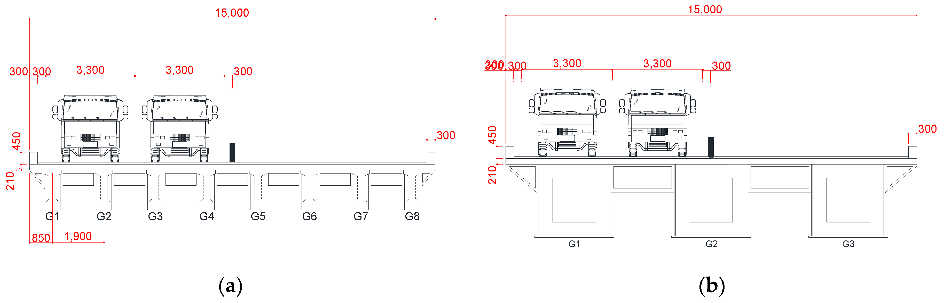
In this study, MIDAS (Civil 2012, MIDAS Information Technology, Seongnam-si, Korea) and MATLAB (2012b, MathWorks, Natick, MA, USA) were used. MIDAS is a FEM (Finite Element Method) program that was used to calculate the design load and transverse distribution coefficient [22]. MATLAB was used to perform various simulations. Table 10 summarizes the extreme vehicle load effects simulated for various traffic environments and three different bridge types [22]: the 30-m-long pre-stressed concrete (PSC) I-girder bridge (Figure 5a), 45-m-long steel box girder bridge (Figure 5b), and 60-m-long steel box girder bridge with a plan view similar to that of the second type. Each bridge type was 15 m wide, four lanes, two-way, and simply-supported single spans. The extreme values in Table 10 were normalized with the current design vehicle load effects first and then renormalized with a reference value for the case with an ADT of 20,000 vehicles on two lanes in one direction and an ADTT of 25%; this was assumed to be the representative traffic environment for national highways in Korea.
As presented in Table 10, two different heavy vehicle distribution models were simulated. The distribution ratio is the heavy vehicle traffic volume ratio of the inner lane to the outer lane. An even distribution of heavy vehicles in two lanes may cause a stronger load effect because of the increased chance that two heavy vehicles run side-by-side for the short-span bridges. However, long-span bridges, such as the 60-m-long bridge, may experience slightly higher load effects with consecutive heavy vehicles in one lane. The extreme values ranged from 0.725 to 1.094 for the 45-m span and from 0.606 to 1.095 for the 60-m span.
5. Conclusions
In this study, the girder type, vehicle type, vehicle weight, and consecutive vehicle characteristics were analyzed by collecting data on vehicle loads and traffic characteristics for national highways, and a rational probabilistic model was developed that reflects actual traffic characteristics. A simulation technique is presented for analyzing the effects of extreme vehicle loads on the superstructures of highway bridges based on the developed vehicle traffic models. Based on the presented technique, a rational plan is proposed to estimate the vehicle load for assessing the required load capacity that reflects the structural characteristics and traffic environment of the bridge based on the extreme load effect over the expected service life and various vehicle traffic and structural characteristics. The conclusions are as follows:
(1) A procedure is presented for determining the vehicle load for a required load capacity assessment that rationally reflects the structural characteristics and traffic environment of a bridge over its expected remaining service life. This will allow for economical maintenance while satisfying the required performance of the target bridge.
(2) To verify the effect of consecutive traveling vehicle characteristics on the proportion of heavy vehicles, models using the consecutive traveling coefficient and proportion of single vehicles were compared regarding the average daily traffic volume per lane of 30- and 60-m-long simply supported bridge with 2000–40,000 vehicles and a heavy vehicle proportion of 15–45%. The annual extreme load effect was set to a non-exceedance probability of 95%. The results showed that the consecutive vehicle effect generally increased by 20–30% for the 30-m span. When the span was longer, this effect was greatly magnified. Depending on the average daily traffic volume and proportion of heavy vehicles, this effect increased by as much as 50%.
(3) The analysis of the extreme load effect according to the traffic environment for three different bridge types (30-m-long PSC I-type girder bridge, 45-m-long steel box girder bridge, and 60-m-long steel box girder bridge) showed that the extreme load effect tended to increase in proportion to the average daily traffic volume and heavy vehicle proportion. Even when the same bridge was analyzed, the extreme value ranged from 0.725 to 1.094 for the 45-m span, and from 0.606 to 1.095 for the 60-m span, depending on the traffic volume and heavy vehicle proportion. This indicates that bridges with various traffic environments can adequately satisfy their target required performance, even if the distribution of bridge maintenance is adjusted upwardly or downwardly for improved efficiency.
Acknowledgments
This study was supported by a Creative Human Resources Center for Resilient Infrastructure grant funded by Yonsei University.
Author Contributions
Sang-Hyo Kim proposed the topic of this study and designed the process; Won-Ho Heo and Dong-woo You performed the simulations; and Jae-Gu Choi performed the analysis and wrote the paper.
Conflicts of Interest
The authors declare no conflict of interest.
References
- Wisniewski, D.F.; Cruz, P.J.S.; Henriques, A.A.R.; Simões, R.A. Probabilistic models for mechanical properties of concrete, reinforcing steel and prestressing steel. Struct. Infrastruct. Eng. 2012, 8, 111–123. [Google Scholar] [CrossRef]
- Korea Ministry of Land, Infrastructure and Transport. Road Bridge and Tunnel Statistics; Ministry of Land, Infrastructure and Transport: Seoul, Korea, 2015.
- González, A.; Rattigan, P.; O’Brien, E.J.; Caprani, C. Determination of bridge lifetime dynamic amplification factor using finite element analysis of critical loading scenarios. Eng. Struct. 2008, 30, 2330–2337. [Google Scholar] [CrossRef]
- Gu, Y.; Li, S.; Li, H.; Guo, Z. A novel Bayesian extreme value distribution model of vehicle loads incorporating de-correlated tail fitting: Theory and application to the Nanjing 3rd Yangtze River Bridge. Eng. Struct. 2014, 59, 386–392. [Google Scholar] [CrossRef]
- O’Brien, E.J.; Schmidt, F.; Hajializadeh, D.; Zhou, X.Y.; Enright, B.; Caprani, C.C.; Sheils, E. A review of probabilistic methods of assessment of load effects in bridges. Struct. Saf. 2015, 53, 44–56. [Google Scholar] [CrossRef]
- O’Connor, A.; O’Brien, E.J. Traffic load modelling and factors influencing the accuracy of predicted extremes. Can. J. Civ. Eng. 2005, 32, 270–278. [Google Scholar] [CrossRef]
- O’Brien, E.J.; Hayrapetova, A.; Walsh, C. The use of micro-simulation for congested traffic load modeling of medium- and long-span bridges. Struct. Infrastruct. Eng. 2012, 8, 269–276. [Google Scholar] [CrossRef]
- Getachew, A.; O’Brien, E.J. Simplified site-specific traffic load models for bridge assessment. Struct. Infrastruct. Eng. 2007, 3, 303–311. [Google Scholar] [CrossRef]
- O’Brien, E.J.; Rattigan, P.; Gonzalez, A.; Dowling, J.; Znidaric, A. Characteristic dynamic traffic load effects in bridges. Eng. Struct. 2009, 31, 1607–1612. [Google Scholar] [CrossRef]
- Fiorillo, G.; Ghosn, M. Application of influence lines for the ultimate capacity of beams under moving loads. Eng. Struct. 2015, 103, 125–133. [Google Scholar] [CrossRef]
- Nowak, A.S.; Park, C.-H.; Casas, J.R. Reliability analysis of prestressed concrete bridge girders: Comparison of Eurocode, Spanish Norma IAP and AASHTO LRFD. Struct. Saf. 2001, 23, 331–344. [Google Scholar] [CrossRef]
- Herrmann, A.W. ASCE 2013 report card for America’s infrastructure. IABSE Symp. Rep. 2013, 99, 9–10. [Google Scholar] [CrossRef]
- Korea Ministry of Land, Transport and Maritime Affairs. Road Traffic Survey Guide, Government Document Registration; Ministry of Land, Transport and Maritime Affairs: Seoul, Korea, 2015.
- Kim, S.-H.; Park, H.-S. A study on bridge live loads and traffic modes. Korea Soc. Civ. Eng. 1992, 12, 107–116. [Google Scholar]
- Bruls, J.M.; Sedlacek, G. Traffic data of the European countries 2nd draft. In Eurocode on Actions; European Committee for Standardization: Brussels, Belgium, 1989. [Google Scholar]
- Kwon, S.-M.; Suh, Y.-C. Development and application of the high speed weigh-in-motion for overweight enforcement. J. Korean Soc. Road Eng. 2009, 11, 69–78. [Google Scholar]
- Korea Infrastructure Safety and Technology Corporation. Development of Bridge Maintenance Technique Considering Performance Based on the Site Environment; Korea Infrastructure Safety and Technology Corporation: Seoul, Korea, 2015. [Google Scholar]
- Gumbel, E.J. Statistics of Extremes; Columbia University Press: New York, NY, USA, 1958. [Google Scholar]
- Enright, B.; O’Brien, E.J. Monte Carlo simulation of extreme traffic loading on short and medium span bridges. Struct. Infrastruct. Eng. 2013, 9, 1267–1282. [Google Scholar] [CrossRef]
- Hwang, E.-S.; Nowak, A.S. Simulation of dynamic load for bridges. J. Struct. Eng. (ASCE) 1991, 117, 1413–1434. [Google Scholar] [CrossRef]
- Korea Institute of Bridge and Structural Engineers. Korea Highway Bridge Specifications; Korea Institute of Bridge and Structural Engineers: Seoul, Korea, 2015. [Google Scholar]
- Kim, S.-H.; Choi, J.-G.; Ham, S.-M.; Heo, W.-H. Reliability evaluation of a PSC highway bridge based on resistance capacity degradation due to corrosive environments. Appl. Sci. 2016, 6, 423–439. [Google Scholar] [CrossRef]
Figure 1.
The number of bridges in Korea according to the year of construction completion.

Figure 2.
Distributions of the load effect under different traffic conditions: (a) normal; (b) severe; and (c) mild.
Figure 2.
Distributions of the load effect under different traffic conditions: (a) normal; (b) severe; and (c) mild.

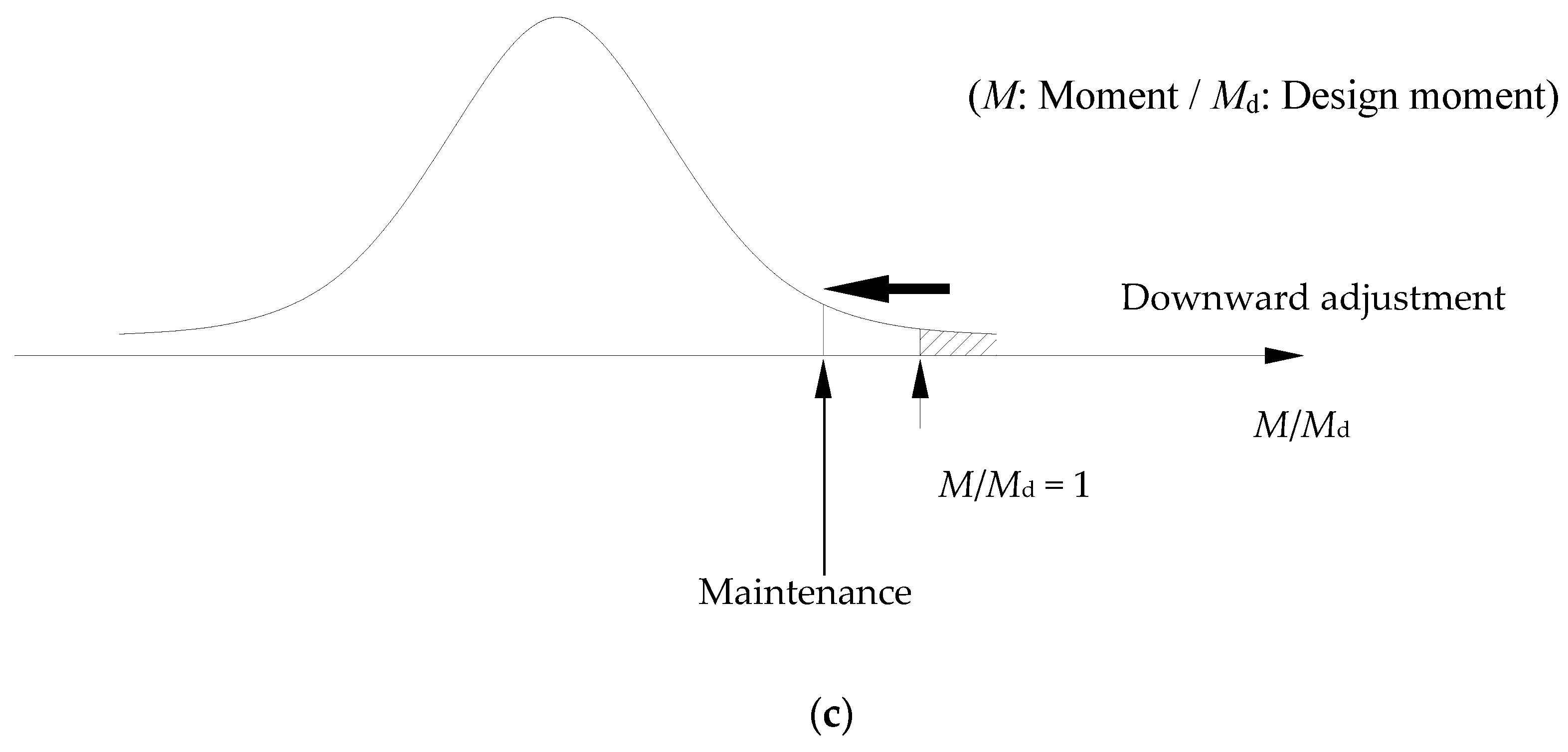
Figure 3.
Load effect of consecutive heavy vehicles.
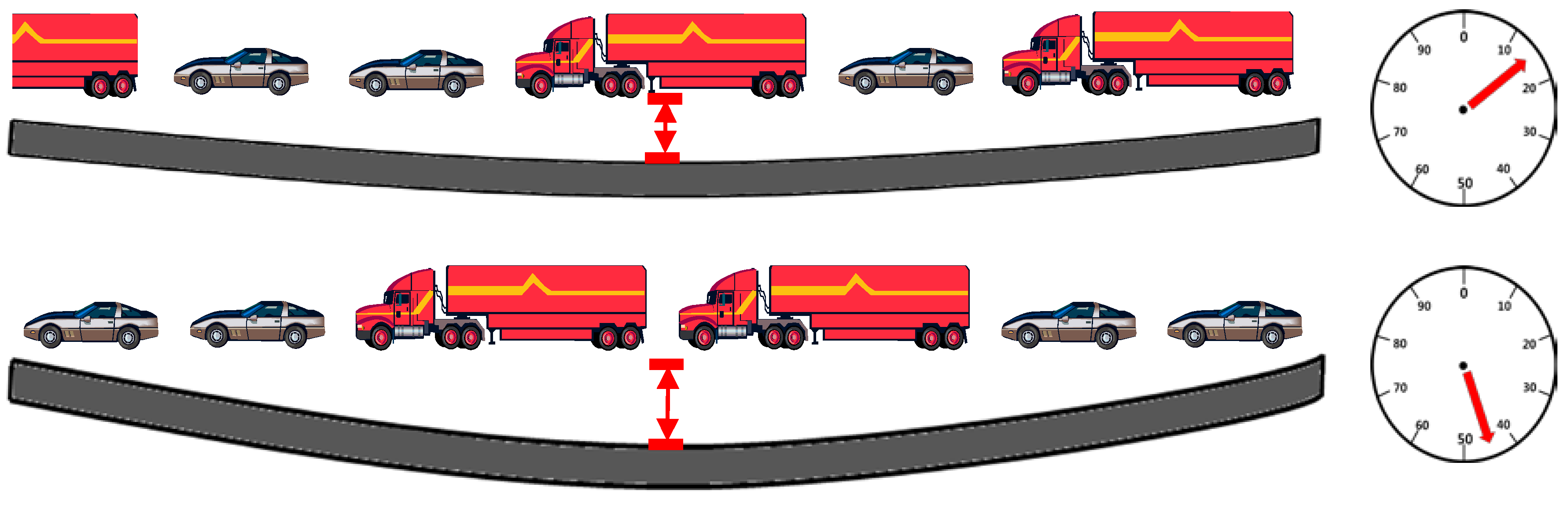
Figure 4.
Probabilistic characteristics of the proposed vehicle weight models: (a) P type; (b) B type; (c) T type; (d) TT type; and (e) ST type.
Figure 4.
Probabilistic characteristics of the proposed vehicle weight models: (a) P type; (b) B type; (c) T type; (d) TT type; and (e) ST type.
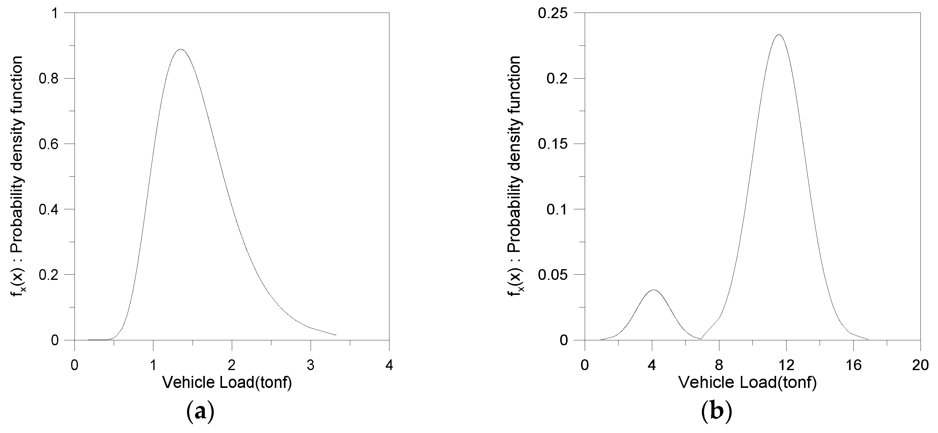

Figure 5.
Target bridge section properties at the mid-span (mm): (a) PSC I-type girder; and (b) steel box girder.
Figure 5.
Target bridge section properties at the mid-span (mm): (a) PSC I-type girder; and (b) steel box girder.


Table 1.
Classification of vehicles.
| Vehicle Model | Vehicle Class * | Description | Feature | Tandem Configuration |
|---|---|---|---|---|
| P | 1 | Mobile car |  |  |
| B | 2 | Bus |  |  |
| T | 3 | Small truck A |  |  |
| 4 | Small truck B |  |  | |
| TT | 5 | Mid-sized truck A |  |  |
| 6 | Mid-sized truck B |  |  | |
| 7 | Mid-sized truck C |  |  | |
| ST | 8 | Heavy truck A |  |  |
| 9 | Heavy truck B |  |  | |
| 10 | Heavy truck C |  |  | |
| 11 | Heavy truck D |  |  | |
| 12 | Heavy truck E |  |  |
* Vehicle class indicates the vehicle classifications presented by [13].
Table 2.
Load distributions and dimensions of the vehicle models.
| Axle Configuration | |||||||
|---|---|---|---|---|---|---|---|
 | |||||||
| Vehicle model | W1 | W2 | W3 | Lf | L1 | L2 | Lr |
| P | 50% | 50% | - | 1.0 m | 2.5 m | - | 1.0 m |
| B | 40% | 60% | - | 2.0 m | 5.5 m | - | 3.0 m |
| T | 30% | 70% | - | 1.5 m | 4.5 m | - | 2.0 m |
| TT | 20% | 80% | - | 1.5 m | 5.0 m | - | 3.0 m |
| ST | 10% | 45% | 45% | 1.5 m | 3.8 m | 8.2 m | 2.0 m |
Table 3.
Probabilistic characteristics of the previous vehicle weight models [14].
Table 3.
Probabilistic characteristics of the previous vehicle weight models [14].
| Vehicle Model | Mode | Dist. Type | Coefficients | Minimum (tonf) | Maximum (tonf) | Correction Coefficients | |
|---|---|---|---|---|---|---|---|
| (Normal) (L-N) | (Normal) (L-N) | ||||||
| P | 1 | L-N | 0.398 | 0.317 | 0.7 | 5.0 | 1.0 |
| B | 1 | Normal | 4.089 | 1.020 | 1.4 | 17.1 | 0.098 |
| 2 | Normal | 11.552 | 1.542 | 4.0 | 24.0 | 0.902 | |
| T | 1 | L-N | 1.338 | 0.620 | 1.25 | 24.1 | 0.733 |
| 2 | L-N | 2.721 | 0.221 | 1.25 | 24.1 | 0.267 | |
| 3 | L-N | 2.490 | 0.260 | 23.5 | 40.0 | 1.0 | |
| TT | 1 | L-N | 2.467 | 0.178 | 7.3 | 41.3 | 0.219 |
| 2 | L-N | 3.253 | 0.203 | 7.3 | 41.3 | 0.781 | |
| 3 | L-N | 3.240 | 0.210 | 41.3 | 65.0 | 1.0 | |
| ST | 1 | Normal | 18.541 | 3.000 | 11.3 | 63.4 | 0.260 |
| 2 | L-N | 3.650 | 0.202 | 11.3 | 63.4 | 0.740 | |
| 3 | L-N | 3.420 | 0.260 | 59.7 | 105.0 | 1.0 | |
L-N: lognormal.
Table 4.
Overloaded vehicle data (2011–2013).
| Region I | Region II | Region III | Region IV | Region V | Region VI | Region VII | |
|---|---|---|---|---|---|---|---|
| 40–50 tons | 1410 | 611 | 302 | 220 | 1440 | 128 | 79 |
| 50–60 tons | 176 | 28 | 72 | 52 | 141 | 3 | 4 |
| 60–70 tons | 55 | 20 | 38 | 28 | 107 | 2 | 6 |
| 70–80 tons | 16 | 9 | 11 | 15 | 32 | 0 | 3 |
| 80–90 tons | 8 | 0 | 5 | 4 | 7 | 0 | 1 |
| Sum | 1665 | 668 | 428 | 319 | 1727 | 133 | 93 |
| Maximum (tonf) | 87.7 | 77.0 | 85.6 | 84.0 | 88.9 | 61.0 | 82.7 |
Table 5.
Probabilistic characteristics of the proposed vehicle weight models.
| Vehicle Model | Mode | Dist. Type | Coefficients | Minimum (tonf) | Maximum (tonf) | Correction Coefficients | |
|---|---|---|---|---|---|---|---|
| (Normal) (L-N) | (Normal) (L-N) | ||||||
| P | 1 | L-N | 0.398 | 0.317 | 0.7 | 5.0 | 1.0 |
| B | 1 | Normal | 4.089 | 1.020 | 1.4 | 17.1 | 0.098 |
| 2 | Normal | 11.552 | 1.542 | 4.0 | 24.0 | 0.902 | |
| T | 1 | L-N | 1.338 | 0.620 | 1.25 | 24.1 | 0.733 |
| 2 | L-N | 2.721 | 0.221 | 1.25 | 24.1 | 0.267 | |
| TT | 1 | L-N | 2.467 | 0.178 | 7.3 | 41.3 | 0.219 |
| 2 | L-N | 3.253 | 0.203 | 7.3 | 41.3 | 0.781 | |
| ST | 1 | Normal | 18.541 | 3.000 | 11.3 | 63.4 | 0.260 |
| 2 | L-N | 3.650 | 0.202 | 11.3 | 90.0 | 0.740 | |
L-N: lognormal.
Table 6.
Vehicle traffic volume of each lane and vehicle type per location.
| Location | Time | Lane | P Type | B Type | T, TT, ST Types | Traffic Volume | Heavy Vehicle Proportion | |
|---|---|---|---|---|---|---|---|---|
| 1 | 7–9 a.m., 2–6 p.m. | 1 | 915 | 9 | 388 | 1312 | 29.6% | 30.1% |
| 2 | 1156 | 57 | 531 | 1744 | 30.4% | |||
| 2 | 7–9 a.m., 2–6 p.m. | 1 | 1584 | 37 | 439 | 2060 | 21.3% | 34.3% |
| 2 | 1239 | 27 | 1070 | 2336 | 45.8% | |||
| 3 | 7–9 a.m., 2–6 p.m. | 1 | 1408 | 19 | 643 | 2070 | 31.1% | 45.7% |
| 2 | 721 | 9 | 1176 | 1906 | 61.7% | |||
| 4 | 7–9 a.m., 1–3 p.m., 5–7 p.m. | 1 | 1329 | 5 | 446 | 1780 | 25.1% | 42.2% |
| 2 | 772 | 9 | 848 | 1629 | 52.1% | |||
| 5 | 7–9 a.m., 1–3 p.m., 5–7 p.m. | 1 | 3445 | 55 | 1122 | 4622 | 24.3% | 31.0% |
| 2 | 1740 | 148 | 1304 | 3192 | 40.9% | |||
Table 7.
Traveling patterns of vehicles.
| Speed | Average Daily Traffic Volume (Two Lanes) | Headway Distance | |||
|---|---|---|---|---|---|
| 5000 | 10,000 | 20,000 | 40,000 | ||
| Below 10 km/h | 5% | 10% | 10% | 15% | 2 m |
| 10–30 km/h | 10% | 20% | 30% | 40% | 5 m |
| 30–50 km/h | 50% | 50% | 40% | 30% | 15 m |
| Above 50 km/h | 35% | 20% | 20% | 15% | 25 m |
Table 8.
Consecutive traveling vehicle model coefficients.
| (a) Heavy vehicle proportion: 15% | |||||||
| Type | Consecutive Traveling Coefficient (Consecutive Traveling Probability: %) | Simple Vehicle Proportion (%) | |||||
| P | B | T | TT | ST | |||
| P | 1.03 | 0.95 | 0.89 | 0.86 | 0.88 | 81.6 | |
| (83.68) | (3.23) | (6.64) | (4.88) | (1.58) | |||
| B | 0.95 | 2.29 | 0.88 | 1.09 | 0.89 | 3.4 | |
| (77.74) | (7.80) | (6.62) | (6.23) | (1.61) | |||
| T | 0.88 | 1.00 | 1.92 | 1.40 | 1.31 | 7.5 | 15.0 |
| (71.87) | (3.39) | (14.42) | (7.96) | (2.37) | |||
| TT | 0.87 | 0.93 | 1.36 | 2.28 | 1.51 | 5.7 | |
| (70.88) | (3.17) | (10.22) | (13.00) | (2.72) | |||
| ST | 0.85 | 1.03 | 1.42 | 1.67 | 3.92 | 1.8 | |
| (69.27) | (3.51) | (10.67) | (9.50) | (7.05) | |||
| (b) Heavy vehicle proportion: 25% | |||||||
| Type | Consecutive Traveling Coefficient (Consecutive Traveling Probability: %) | Simple Vehicle Proportion (%) | |||||
| P | B | T | TT | ST | |||
| P | 1.06 | 0.97 | 0.85 | 0.80 | 0.83 | 72.0 | |
| (76.36) | (2.92) | (10.59) | (7.64) | (2.49) | |||
| B | 0.98 | 2.32 | 0.83 | 1.02 | 0.84 | 3.0 | |
| (70.40) | (6.97) | (10.43) | (9.68) | (2.52) | |||
| T | 0.84 | 0.94 | 1.71 | 1.27 | 1.16 | 12.5 | 25.0 |
| (60.33) | (2.82) | (21.32) | (12.05) | (3.48) | |||
| TT | 0.83 | 0.88 | 1.20 | 1.98 | 1.35 | 9.5 | |
| (59.47) | (2.63) | (15.01) | (18.84) | (4.04) | |||
| ST | 0.80 | 0.97 | 1.25 | 1.45 | 3.43 | 3.0 | |
| (57.39) | (2.90) | (15.66) | (13.75) | (10.30) | |||
| (c) Heavy vehicle proportion: 35% | |||||||
| Type | Consecutive Traveling Coefficient (Consecutive Traveling Probability: %) | Simple Vehicle Proportion (%) | |||||
| P | B | T | TT | ST | |||
| P | 1.11 | 1.01 | 0.83 | 0.77 | 0.82 | 62.4 | |
| (69.10) | (2.62) | (14.58) | (10.28) | (3.43) | |||
| B | 1.01 | 2.38 | 0.81 | 0.97 | 0.81 | 2.6 | |
| (63.31) | (6.20) | (14.19) | (12.88) | (3.42) | |||
| T | 0.82 | 0.90 | 1.53 | 1.17 | 1.03 | 17.5 | 35.0 |
| (51.02) | (2.34) | (26.79) | (15.53) | (4.31) | |||
| TT | 0.81 | 0.84 | 1.08 | 1.76 | 1.21 | 13.3 | |
| (50.29) | (2.18) | (18.98) | (23.47) | (5.08) | |||
| ST | 0.77 | 0.93 | 1.12 | 1.28 | 3.08 | 4.2 | |
| (48.06) | (2.41) | (19.62) | (16.98) | (12.94) | |||
| (d) Heavy vehicle proportion: 45% | |||||||
| Type | Consecutive Traveling Coefficient (Consecutive Traveling Probability: %) | Simple Vehicle Proportion (%) | |||||
| P | B | T | TT | ST | |||
| P | 1.21 | 1.09 | 0.84 | 0.77 | 0.82 | 52.8 | |
| (62.02) | (2.33) | (18.45) | (12.87) | (4.33) | |||
| B | 1.09 | 2.54 | 0.81 | 0.96 | 0.81 | 2.2 | |
| (56.37) | (5.45) | (17.85) | (16.04) | (4.29) | |||
| T | 0.83 | 0.90 | 1.45 | 1.10 | 0.97 | 22.5 | 45.0 |
| (42.59) | (1.93) | (31.96) | (18.37) | (5.14) | |||
| TT | 0.81 | 0.84 | 1.03 | 1.66 | 1.14 | 17.1 | |
| (41.87) | (1.80) | (22.60) | (27.70) | (6.03) | |||
| ST | 0.77 | 0.92 | 1.06 | 1.19 | 2.90 | 5.4 | |
| (39.67) | (1.97) | (23.19) | (19.90) | (15.27) | |||
Table 9.
Comparison of simple and consecutive running models (95% annual maximum).
| Span | Heavy Vehicle Proportion | Model | Average Daily Traffic Volume | ||||
|---|---|---|---|---|---|---|---|
| 2000 | 5000 | 10,000 | 20,000 | 40,000 | |||
| 30 m | 15% | Simple | 1.29 | 1.34 | 1.35 | 1.39 | 1.43 |
| Consecutive | 1.55 | 1.61 | 1.65 | 1.67 | 1.72 | ||
| Consecutive model effect | 20.8% ↑ | 20.2% ↑ | 22.5% ↑ | 20.2% ↑ | 20.1% ↑ | ||
| 25% | Simple | 1.29 | 1.36 | 1.38 | 1.41 | 1.47 | |
| Consecutive | 1.57 | 1.69 | 1.71 | 1.73 | 1.74 | ||
| Consecutive model effect | 21.7% ↑ | 24.9% ↑ | 24.0% ↑ | 22.2% ↑ | 18.2% ↑ | ||
| 35% | Simple | 1.32 | 1.36 | 1.41 | 1.41 | 1.48 | |
| Consecutive | 1.57 | 1.74 | 1.79 | 1.83 | 1.83 | ||
| Consecutive model effect | 19.4% ↑ | 27.7% ↑ | 27.5% ↑ | 29.4% ↑ | 24.1% ↑ | ||
| 45% | Simple | 1.33 | 1.38 | 1.43 | 1.46 | 1.49 | |
| Consecutive | 1.58 | 1.76 | 1.86 | 1.91 | 2.00 | ||
| Consecutive model effect | 18.7% ↑ | 27.8% ↑ | 30.4% ↑ | 30.9% ↑ | 34.8% ↑ | ||
| 60 m | 15% | Simple | 1.41 | 1.47 | 1.48 | 1.53 | 1.58 |
| Consecutive | 1.74 | 2.02 | 2.11 | 2.16 | 2.15 | ||
| Consecutive model effect | 23.0% ↑ | 37.1% ↑ | 42.5% ↑ | 41.2% ↑ | 36.3% ↑ | ||
| 25% | Simple | 1.42 | 1.49 | 1.52 | 1.55 | 1.62 | |
| Consecutive | 1.75 | 2.25 | 2.29 | 2.35 | 2.36 | ||
| Consecutive model effect | 23.2% ↑ | 50.7% ↑ | 51.1% ↑ | 51.4% ↑ | 45.9% ↑ | ||
| 35% | Simple | 1.45 | 1.50 | 1.54 | 1.55 | 1.62 | |
| Consecutive | 1.80 | 2.28 | 2.30 | 2.35 | 2.40 | ||
| Consecutive model effect | 23.9% ↑ | 52.1% ↑ | 49.0% ↑ | 51.4% ↑ | 48.4% ↑ | ||
| 45% | Simple | 1.46 | 1.51 | 1.57 | 1.60 | 1.63 | |
| Consecutive | 1.80 | 2.32 | 2.31 | 2.36 | 2.47 | ||
| Consecutive model effect | 23.6% ↑ | 53.5% ↑ | 47.0% ↑ | 47.7% ↑ | 51.7% ↑ | ||
Table 10.
Annual extreme load effects due to different traffic environments (95% annual maximum).
| Annual Extreme Load Effects | |||||||
|---|---|---|---|---|---|---|---|
| Girder Type | Heavy Vehicle Distribution | Heavy Vehicle Proportion | Average Daily Traffic Volume (Two Lanes) | ||||
| 2000 | 5000 | 10,000 | 20,000 | 40,000 | |||
| PSC-I 30 m | 50:50 | 15% | 0.849 | 0.941 | 0.948 | 0.960 | 0.974 |
| 25% | 0.876 | 0.983 | 0.993 | 1.000 | 1.024 | ||
| 35% | 0.886 | 1.002 | 1.020 | 1.024 | 1.027 | ||
| 45% | 0.893 | 1.034 | 1.041 | 1.046 | 1.060 | ||
| 15:85 | 15% | 0.812 | 0.906 | 0.920 | 0.939 | 0.945 | |
| 25% | 0.835 | 0.934 | 0.982 | 0.986 | 0.996 | ||
| 35% | 0.857 | 0.976 | 0.996 | 0.999 | 1.010 | ||
| 45% | 0.868 | 1.011 | 1.016 | 1.029 | 1.046 | ||
| STB 45 m | 50:50 | 15% | 0.740 | 0.930 | 0.936 | 0.960 | 0.966 |
| 25% | 0.756 | 0.970 | 0.983 | 1.000 | 1.020 | ||
| 35% | 0.769 | 1.031 | 1.040 | 1.043 | 1.055 | ||
| 45% | 0.781 | 1.048 | 1.059 | 1.082 | 1.094 | ||
| 15:85 | 15% | 0.725 | 0.872 | 0.905 | 0.913 | 0.927 | |
| 25% | 0.750 | 0.936 | 0.964 | 0.972 | 0.979 | ||
| 35% | 0.761 | 0.987 | 0.993 | 1.010 | 1.010 | ||
| 45% | 0.772 | 1.017 | 1.032 | 1.041 | 1.045 | ||
| STB 60 m | 50:50 | 15% | 0.672 | 0.932 | 0.943 | 0.949 | 0.965 |
| 25% | 0.680 | 0.983 | 0.990 | 1.000 | 1.015 | ||
| 35% | 0.689 | 1.036 | 1.072 | 1.077 | 1.083 | ||
| 45% | 0.701 | 1.077 | 1.091 | 1.093 | 1.095 | ||
| 15:85 | 15% | 0.606 | 0.869 | 0.877 | 0.889 | 0.906 | |
| 25% | 0.626 | 0.957 | 0.974 | 0.977 | 0.980 | ||
| 35% | 0.649 | 1.006 | 1.015 | 1.015 | 1.019 | ||
| 45% | 0.680 | 1.034 | 1.045 | 1.047 | 1.055 | ||
© 2017 by the authors. Licensee MDPI, Basel, Switzerland. This article is an open access article distributed under the terms and conditions of the Creative Commons Attribution (CC BY) license (http://creativecommons.org/licenses/by/4.0/).
Share and Cite
MDPI and ACS Style
Kim, S.-H.; Heo, W.-H.; You, D.-w.; Choi, J.-G. Vehicle Loads for Assessing the Required Load Capacity Considering the Traffic Environment. Appl. Sci. 2017, 7, 365. https://doi.org/10.3390/app7040365
AMA Style
Kim S-H, Heo W-H, You D-w, Choi J-G. Vehicle Loads for Assessing the Required Load Capacity Considering the Traffic Environment. Applied Sciences. 2017; 7(4):365. https://doi.org/10.3390/app7040365
Chicago/Turabian StyleKim, Sang-Hyo, Won-Ho Heo, Dong-woo You, and Jae-Gu Choi. 2017. "Vehicle Loads for Assessing the Required Load Capacity Considering the Traffic Environment" Applied Sciences 7, no. 4: 365. https://doi.org/10.3390/app7040365
Note that from the first issue of 2016, this journal uses article numbers instead of page numbers. See further details here.