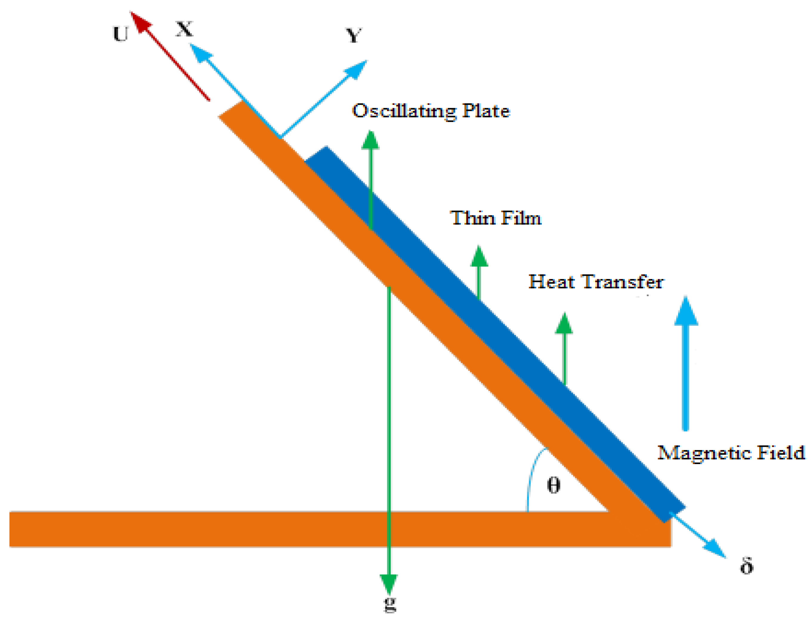
Heat Transfer Investigation of the Unsteady Thin Film Flow of Williamson Fluid Past an Inclined and Oscillating Moving Plate

Abstract

This investigation aims at analyzing the thin film flow passed over an inclined moving plate. The differential type non-Newtonian fluid of Williamson has been used as a base fluid in its unsteady state. The physical configuration of the oscillatory flow pattern has been demonstrated and especial attention has been paid to the oscillatory phenomena. The shear stresses have been combined with the energy equation. The uniform magnetic field has been applied perpendicularly to the flow field. The principal equations for fluid motion and temperature profiles have been modeled and simplified in the form of non-linear partial differential equations. The non-linear differential equations have been solved with the help of a powerful analytical technique known as Optimal Homotopy Asymptotic Method (OHAM). This method contains unknown convergence controlling parameters $C_1,C_2,C_3,...$ which results in more efficient and fast convergence as compared to other analytical techniques. The OHAM results have been verified by using a second method known as Adomian Decomposition Method (ADM). The closed agreement of these two methods and the fast convergence of OHAM has been shown graphically and numerically. The comparison of the present work and published work has also been equated graphically and tabulated with absolute error. Moreover, the effect of important physical parameters like magnetic parameter $M$, gravitational parameter $m$, Oscillating parameter $\omega$, Eckert number $Ec$ and Williamson number $We$ have also been derived and discussed in this article.

1. Introduction

Thin-film flows have various applications in the fields of engineering and industry. In chemical engineering, thin film layers have an effective role in the developments of thin-film reactors, distillation columns, condensers and evaporators. The huge advantages of a thin layer depends on its minute thickness, which provides its flow through micro channels. Thin film layers have vital roles in physical engineering and have broad applications in providing cooling methods for nanotechnology through heat sinks. In geophysical engineering, a lot of problems emerge related to thin film flows such as mudslides, debris flows and lava [1,2]. In the available literature, studies of thin film flows are mostly related to Newtonian fluids and very little work has been done related to non-Newtonian fluids. These too are of great importance, as shear-thickening and pseudoplastic or shear-thinning fluids are considered to be in the class of non-Newtonian fluids. The studies of thin film flow of shear-thinning fluids have vast importance in the industries involving photographic films and the extrusion of polymer sheets, etc. The behavior of pseudoplastic fluids has been explained comprehensively in the Ostwald de Waele power law, Cross, Carreaus and Ellis models, but little attention has been given to the Williamson fluid model. The flow of pseudoplastic fluids has been experimentally described by Williamson [3], with verified results. Dapra and Scarpi [4] have discussed the analytical solution of Williamson fluid by using the perturbation technique. Most of the problems related to Williamson fluid have been modeled in steady state. Very little work has been done on unsteady non-Newtonian fluids. Gamal and Rahman [5] have discussed the unsteady magnetohydrodynamic flow of non-Newtonian fluids obeying the power law model. Khan [6] has discussed Williamson fluid flow using scaling transformation. Hayat et al. [7] have studied the Williamson fluid flow on a stretching cylinder with thermal radiations and Ohmic dissipation. Nadeem et al. [8] have discussed the Williamson fluid flow on a stretching surface. They studied the effect of physical parameters involved in the problem. Waris et al. [9] have investigated the nanofluid study of the thin film Williamson fluid flow on a stretching surface. Abdollahzadeh Jamalabadi et al. [10] have examined the numerical simulation of Williamson fluid flow amongst binary parallel vertical Walls with slip effects. Thin film nanofluid spray on the stretching cylinder surface has been examined by Noor et al. [11]. The spray rate under the applied pressure force has been scrutinized in their study. Gul et al. [12] have discussed the variable properties of thin layer third order differential type fluid. Miladinova et al. [13] and Siddiqui et al. [14] have studied the thin film flow of non-Newtonian fluids using different geometries. The unsteady fluid problems have been evaluated in the study of Fetecau [15]. The similar study of fluid flows in its unsteady state can also be seen in [16,17,18,19].

The fluid flow with oscillatory physical conditions has important applications, such as those that Fatimah and Jaworski [20] have examined in their experimental analysis of the friction factor correlation for a regenerator using oscillatory phenomena in a thermo acoustic system. Huang et al. [21] have experimentally studied the empirical correlation for finned heat exchangers using oscillating analysis. The thin film flow on an oscillatory belt in the field of mechanical engineering has been studied by Gul et al. [22]. Heat transmission in fluid flows has much importance in basic engineering. Still, a lot of work remains to be done regarding oscillatory flow problems. Various applications related to Stirling machines, heat exchangers, pulsed-tube coolers in cryogenics and wire coating have been explored by Shah et al. [23]. Gravity-driven flows may occur in various natural and industrial events, such as the lifting and drainage of fluid flows on a vertical and inclined oscillating plane, as studied by Yongqi et al. [24] and Gul et al. [25,26,27]. Ellahi et al. [28] have studied the oscillating effect of nano-Ferroliquid on a stretchable rotating disk.

For the solution of real world problems, researchers and engineers use numerical [29,30] and analytical [31,32,33,34,35,36] techniques to find the approximate solution of modelled problems. This recent work has been handled analytically using the technique known as Optimal Homotpy Asymptotic Method (OHAM). OHAM is one of the powerful analytical techniques to handle non-linear problems. Marinca and Herisanu [37,38,39] are the founders of OHAM and they applied this method to the problems of thin film and steady flows. Nowadays, most researchers use OHAM for the solution of nonlinear Ordinary Differential Equations (ODEs)and Partial Differential Equations (PDEs). The uses of this method for high non-linear problems can also be seen in the work of Mabood et al. [40].

Considering the above expression, the aim of the current work is to study the thin film flow of Williamson fluid on an oscillating and translated inclined plane in the presence of magnetic and temperature fields using OHAM. The physical study of the magnetic field, gravity term, oscillation parameter and Eckert number is investigated and discussed in this work.

2. Materials and Methods

Consider a flow of thin film Williamson fluid on an inclined plate. The plate is oscillating and moving with a uniform velocity $U$ at time $t=0^{+}$. The thickness of the liquid film is considered uniform and equal to $\delta$. The gravity force opposes the fluid motion and tries to make the fluid film drain down the plate. A uniform magnetic field is applied transversely to the translating inclined plate. Furthermore, during fluid motion, constant temperature filed is also considered. The flow is assumed to be unsteady and laminar after a small distance above the film surface.

The physical conditions of the unsteady problem are used as:

$$u\left(0,t\right)=U\left(1+\cos \omega t\right),\frac{\partial u\left(\delta ,t\right)}{\partial y}=0,$$

(1)

$$\mathrm{\Theta }(0,t)={\mathrm{\Theta }}_0,\mathrm{\Theta }(\delta ,t)={\mathrm{\Theta }}_1,$$

(2)

where $\omega$ is the frequency of the oscillating plate and $\delta$ is the thickness of the thin film.

The Lorentz force $\mathbf{J}\times \mathbf{B}$ for the uniform Magnetic field is defined as:

$$\mathbf{J}\times \mathbf{B}=\left[\mathit{0},-\sigma B_0^{2}u(y,t),\mathit{0}\right],$$

(3)

where $\sigma$ is the electrical conductivity of the fluid.

The governing equations take the form as:

$$\nabla .\mathbf{u}=0,$$

(4)

$$\rho \frac{d\mathbf{u}}{dt}=-\nabla p+\rho \mathbf{g}\mathbf{sin}(\mathrm{\Theta })+\nabla .\mathbf{T}+\mathbf{J}\times \mathbf{B},$$

(5)

$$\rho C_p\frac{D\mathrm{\Theta }}{Dt}=k{\nabla }^2\mathrm{\Theta }+tr\left(\mathbf{T}\mathbf{.}\mathbf{L}\right),$$

(6)

where $\mathbf{u}$ is the velocity vector, $\rho$ is the fluid density, $\mathbf{g}$ is the gravity force, $p$ is the pressure term, $\mathrm{\Theta }$ is the temperature field, $k$ defines thermal conductivity, $C_p$ is the specific heat and $\mathbf{L}=\nabla \mathbf{u}$.

The extra stress tensor $\mathbf{T}$ for the Williamson fluid is defined as in [4,8]:

$$\mathbf{T}=\left[{\mu }_{\mathrm{\infty }}+\left({\mu }_0+{\mu }_{\mathrm{\infty }}\right){\left(1-\mathrm{\Gamma }\dot{\mathsf{\gamma }}\right)}^{-1}\right]\dot{\mathsf{\gamma }},$$

(7)

where $\mathrm{\Gamma }$ is the time constant, ${\mu }_0$ is the zero viscosity, ${\mu }_{\mathrm{\infty }}$ is the infinite viscosity, and $\dot{\mathsf{\gamma }}$ is defined as:

$$\dot{\mathsf{\gamma }}=\sqrt{\frac{1}{2}{\displaystyle \sum _i{\displaystyle \sum _j{\gamma }_{ij}{\gamma }_{ji}}}}=\sqrt{\frac{1}{2}\Pi },$$

(8)

where $\Pi =trace{(A_1)}^2=2{\left(\frac{\partial u}{\partial y}\right)}^2$ is the second invariant strain tensor derived as in [4,8]. We consider the constitutive Equation (7) in which ${\mu }_{\mathrm{\infty }}$ = 0 and $\mathrm{\Gamma }\dot{\mathsf{\gamma }}<1$. The component of the extra stress tensor, therefore, can be written as:

$$\mathbf{T}={\mu }_0\left[{\left(1-\mathrm{\Gamma }\dot{\mathsf{\gamma }}\right)}^{-1}\right]\dot{\mathsf{\gamma }}={\mu }_0\left[\left(1+\mathrm{\Gamma }\dot{\mathsf{\gamma }}\right)\right]\dot{\mathsf{\gamma }},$$

(9)

where $\dot{\mathsf{\gamma }}=\frac{\partial \mathbf{u}}{\partial y}$ is the shear rate and $\mathrm{\Gamma }$ is the time constant. The unsteady unidirectional velocity field and temperature profile is defined as:

$$\mathbf{u}=\left[u(y,t),0,0\right],\mathrm{\Theta }=\mathrm{\Theta }(y,t),$$

(10)

When (9) and (10) are used in (4)–(6), the continuity equation is identically satisfied and the momentum and energy equations without dynamic pressure are reduced to:

$$\rho \frac{\partial u}{\partial t}={\mu }_0\frac{{\partial }^{2}u}{\partial y^2}+{\mu }_0\mathrm{\Gamma }\frac{\partial }{\partial y}{\left(\frac{\partial u}{\partial y}\right)}^2-\rho g\sin (\mathrm{\Theta })-\sigma B_0^{2}u,$$

(11)

$$\rho c_p\left(\frac{\partial \mathrm{\Theta }}{\partial t}\right)=k\frac{{\partial }^2\mathrm{\Theta }}{\partial y^2}+{\mu }_0{\left(\frac{\partial u}{\partial y}\right)}^2+{\mu }_0\mathrm{\Gamma }{\left(\frac{\partial u}{\partial y}\right)}^3,$$

(12)

Introduce the following dimensionless parameters:

$$\begin{array}{l}\overline{u}=\frac{u}{U},\overline{y}=\frac{x}{\delta },\overline{t}=\frac{\mu t}{\rho {\delta }^2},\overline{\mathrm{\Theta }}=\frac{\mathrm{\Theta }-{\mathrm{\Theta }}_0}{{\mathrm{\Theta }}_1-{\mathrm{\Theta }}_0},\overline{\omega }=\frac{\omega {\delta }^2\rho }{\mu },We=\frac{\mathrm{\Gamma }U}{\delta },\\ p_r=\frac{\mu C_p}{k},E_c=\frac{\mu U^2}{k({\mathrm{\Theta }}_1-{\mathrm{\Theta }}_0)},M=\frac{\sigma B_0^2{\delta }^2}{{\mu }_0},m=\frac{{\delta }^2\rho g\sin \mathrm{\Theta }}{\mu U}.\end{array}$$

(13)

Using the above dimensionless parameters from Equation (13) in the governing partial differential Equations (11) and (12) and in the boundary conditions (1,2), we get:

$$\frac{\partial u}{\partial t}=\frac{{\partial }^{2}u}{\partial y^2}+W_e\frac{\partial }{\partial y}{\left(\frac{\partial u}{\partial y}\right)}^2-m-Mu,$$

(14)

$$Pr\left(\frac{\partial \mathrm{\Theta }}{\partial t}\right)=\frac{{\partial }^2\mathrm{\Theta }}{\partial y^2}+E_c{\left(\frac{\partial u}{\partial y}\right)}^2+W_e{E}_c{\left(\frac{\partial u}{\partial y}\right)}^3,$$

(15)

$$u\left(0,t\right)=\left(1+\cos \omega t\right),\frac{\partial u\left(1,t\right)}{\partial t}=0,$$

(16)

$$\mathrm{\Theta }(0,t)=0,\mathrm{\Theta }(1,t)=1.$$

(17)

where $m$, is the gravitational parameter, $W_e$ is the Williamson parameter, $M$ is the magnetic parameter, $Pr$ is the Prandtl number, $E_c$ is the Eckert number, $\omega$ is the oscillating parameter and $t$ is the time parameter.

Solution by OHAM

The boundary value problem is considered to analyze the OHAM method as:

$$L(u(y,t))+N(u(y,t))+g(u(y,t))=0,B(u)=0.$$

(18)

Here $L$ denotes the linear operator of the differential equation, $N$ is used as a non-linear operator, the independent variable is denoted by $y$, $g$ is a source term and $B$ is a boundary operator. According to OHAM, the homotopy is constructed as:

$$[1-q]\left[L\psi (y,t,q)+g(y,t)\right]-H(q)\left[L\psi (y,t,q)+g\psi (y,t,q)+N\psi (y,t,q)\right]=0,$$

(19)

where $q\in \left[0,1\right]$ is an embedding parameter, $H(q)=q{c}_1+q^2{c}_2+...m,$ is an auxiliary function, $c_1,c_2$ are the convergence controlling parameters and $\psi (x,t,q)$ is an unknown function. Obviously, when $q=0$ and $q=1,$ it holds that:

$$\psi (y,t,q)=u_0(y,t),\psi (y,t,\mathit{1})=u(y,t),$$

(20)

$$\psi (y,t,q,c_i)=u_0(y,t)+{\displaystyle {\sum }_{k\ge 1}{u}_k(y,t,c_i)}{q}^k,i=1,2,\mathrm{3...},m,$$

(21)

Implanting Equation (20) in Equation (21), accumulating the similar powers of $q$ and comparing each coefficient of $q$ to zero, the non-linear PDE are solved with the given boundary conditions to get $u_0(y,t),u_1(y,t),u_2(y,t)$.

The general solution of Equation (21) can be written as:

$$u^m=u_0(y,t)+{\displaystyle {\sum }_{k=1}{u}_k(y,t,c_i)},$$

(22)

The coefficients $c_1,c_2,c_3,...,c_m$ are the functions of $y$.

Inserting Equation (22) in Equation (18), the residual is obtained as:

$$R(y,t,c_i)=L\left(u^m(y,t,c_i)\right)+g(y,t)+N\left(u^m(y,t,c_i)\right),$$

(23)

Frequently methods like Ritz Method, Galerkin’s Method, Collocation Method and Method of Least Squares are used to find the optimal values of $c_i,i=1,2,3,\mathrm{4....}$ The current problem is solved through the Method of Least Squares as given below:

$$J(c_1,c_2,c_3,...,c_m)={\displaystyle {\mathsf{\int }}_a^b{R}^2}(y,t,c_1,c_2,c_3,...,c_m)dy,$$

(24)

where $a$ and $b$ are constants and selected from the domain of the problem.

The controlling convergence parameters $({\mathrm{c}}_1,{\mathrm{c}}_2,{\mathrm{c}}_3,...,{\mathrm{c}}_{\mathrm{m}})$ can be obtained from:

$$\frac{\partial J(c_1,c_2,...,c_m)}{\partial c_1}=\frac{\partial J(c_1,c_2,...,c_m)}{\partial c_2}=...=\frac{\partial J(c_1,c_2,...,c_m)}{\partial c_m}=0$$

(25)

Finally, from these controlling convergence parameters, the approximate solution is determined.

The homotopy equation constructed in Equation (18) is applied to Equations (14) and (15) and the like powers of $q$ are equated as:

$$q^o:\frac{{\partial }^2{u}_0}{\partial y^2}=m,$$

(26)

$$\frac{{\partial }^2{\mathrm{\Theta }}_0}{\partial y^2}=0,$$

(27)

$$q^1:\frac{{\partial }^2{u}_1}{\partial y^2}=-m+m{c}_1-M{c}_1{v}_0+c_1\frac{\partial v_0}{\partial t}+\frac{{\partial }^2{v}_0}{\partial y^2}-c_1\frac{{\partial }^2{v}_0}{\partial y^2}+2c_1{W}_e\frac{\partial v_0}{\partial y}\left(\frac{{\partial }^2{v}_0}{\partial y^2}\right),$$

(28)

$$\frac{{\partial }^2{\mathrm{\Theta }}_1}{\partial y^2}=\mathrm{Pr}{c}_3\frac{\partial {\mathrm{\Theta }}_0}{\partial t}+E_c{c}_3{\left(\frac{\partial v_0}{\partial y}\right)}^2-E_c{W}_e{c}_3{\left(\frac{\partial v_0}{\partial y}\right)}^3+\frac{{\partial }^2{\mathrm{\Theta }}_0}{\partial y^2}-c_3\frac{{\partial }^2{\mathrm{\Theta }}_0}{\partial y^2},$$

(29)

$$\begin{array}{l}{q}^2:\frac{{\partial }^2{u}_2}{\partial y^2}=-m{c}_2-M{c}_2{u}_0-c_2\frac{\partial u_0}{\partial t}-M{c}_1{u}_1-c_1\frac{\partial u_1}{\partial t}+c_2\frac{{\partial }^2{u}_0}{\partial y^2}-2W_e{c}_2\left(\frac{\partial u_0}{\partial y}\right)\left(\frac{{\partial }^2{u}_0}{\partial y^2}\right)-\\ 2W_e{c}_1\left(\frac{\partial u_1}{\partial y}\right)\left(\frac{{\partial }^2{u}_0}{\partial y^2}\right)-(1-c_1)\frac{{\partial }^2{u}_1}{\partial y^2}-2W_e{c}_1\left(\frac{\partial u_0}{\partial y}\right)\left(\frac{{\partial }^2{u}_1}{\partial y^2}\right),\end{array}$$

(30)

$$\begin{array}{c}\frac{{\partial }^2{\mathrm{\Theta }}_2}{\partial y^2}=-\mathrm{Pr}{c}_4\frac{\partial {\mathrm{\Theta }}_0}{\partial t}-\mathrm{Pr}{c}_3\frac{\partial {\mathrm{\Theta }}_1}{\partial t}+E_c{c}_4{\left(\frac{\partial u_0}{\partial y}\right)}^2+W_e{E}_c(c_4+c_3)\frac{\partial u_0}{\partial y}{\left(\frac{\partial u_0}{\partial y}\right)}^2+\\ 2E_c{c}_3\frac{\partial u_0}{\partial y}\frac{\partial u_1}{\partial y}+c_4\frac{{\partial }^2{\mathrm{\Theta }}_0}{\partial y^2}+\left(1+c_3\right)\frac{{\partial }^2{\mathrm{\Theta }}_1}{\partial y^2},\end{array}$$

(31)

The zeroth, first and second components solution for the velocity and temperature fields are obtained from Equations (26)–(31) using the boundary conditions from Equations (16) and (17), respectively.

$$u_0(y,t)=1+\mathrm{Cos}(t\omega )-my+\frac{m}{2}{y}^2,$$

(32)

$${\mathrm{\Theta }}_0(y,t)=y,$$

(33)

$$u_1(y,t,c_1)=c_1\left[\left(a_0+a_1\mathrm{Cos}(\omega t)\right)y-\left(a_2+a_3\mathrm{Cos}(\omega t)\right)y^2+\left(a_4+\frac{M}{6}\mathrm{Cos}(\omega t)\right)y^3-\left(c_1\frac{mM}{24}\right)y^4\right],$$

(34)

$$u_2(y,t,c_1)=\left[\begin{array}{l}\left(c_1{b}_0+c_1^2{b}_1+c_1{b}_2\mathrm{Cos}(\omega t)+c_1^2{b}_3\mathrm{Cos}(\omega t)+c_1^2{b}_4\mathrm{Cos}(2\omega t)+c_2{b}_5+c_2{b}_6\mathrm{Cos}(\omega t)\right)y+\\ \left(c_1{b}_7+c_2{b}_8\mathrm{Cos}(\omega t)+c_1^2{b}_9+c_1^2{b}_{10}\mathrm{Cos}(\omega t)+c_1^2{b}_{11}\mathrm{Cos}(2\omega t)+c_2{b}_{12}-c_{2}m{w}_e\mathrm{Cos}(\omega t)\right)y^2+\\ \left(c_1{b}_{13}+c_1\frac{M}{6}\mathrm{Cos}(\omega t)+c_1^2{b}_{14}+c_1^2{b}_{15}\mathrm{Cos}(\omega t)-c_1^2\frac{M{w}_e}{6}\mathrm{Cos}(2\omega t)+c_2{b}_{16}+c_2\frac{M}{6}\mathrm{Cos}(\omega t)\right)y^3\\ \left(-c_1\frac{mM}{24}+c_1^2{b}_{17}+c_1^2{b}_{18}\mathrm{Cos}(\omega t)\right)y^4+\left(\left(\frac{c_1^{2}M}{12}\right)b_{19}\right)y^5+\left(c_1^2\frac{m{M}^2}{720}\right)y^6\end{array}\right],$$

(35)

$$u(y,t,c_1)=1+\mathrm{Cos}(\omega t)+\left[\begin{array}{l}\left(\begin{array}{l}-1-\frac{m}{2}-\mathrm{Cos}(\omega t)+c_1{d}_0+c_1{d}_1\mathrm{Cos}(\omega t)+c_1^2{d}_2+c_1^2{d}_3\mathrm{Cos}(\omega t)+c_1^2{d}_4\mathrm{Cos}(2\omega t)+c_2{d}_5+\\ c_2{d}_6\mathrm{Cos}(\omega t)\end{array}\right)y+\\ \left(\frac{m}{2}+c_1{d}_7+c_1{d}_8\mathrm{Cos}(\omega t)+c_1^2{d}_9+c_1^2{d}_{10}\mathrm{Cos}(\omega t)+c_1^2{d}_{11}\partial \mathrm{Cos}(2\omega t)+c_2{d}_{12}+c_2{d}_{13}\mathrm{Cos}(\omega t)\right)y^2+\\ \left(c_1{d}_{14}+c_1\frac{m}{3}\mathrm{Cos}(\omega t)+c_1^2{d}_{15}+c_1^2{d}_{16}\mathrm{Cos}(\omega t)-c_1^2(\frac{M{w}_e}{6})\mathrm{Cos}(2\omega t)+c_2{d}_{17}+c_2(\frac{m}{6})\mathrm{Cos}(\omega t)\right)y^3+\\ \left((\frac{mM}{12})c_1+c_1^2{b}_{18}+c_1^2{b}_{19}\mathrm{Cos}(\omega t)+(\frac{-mM}{24})c_2\right)y^4+\left(c_1^2{d}_{20}-(\frac{M^2}{120})c_1^2\mathrm{Cos}(\omega t)\right)y^5+\left((\frac{m{M}^2}{720})c_1^2\right)y^6\end{array}\right],$$

(36)

$${\mathrm{\Theta }}_1(y,t)=\left[\begin{array}{l}\left(E_c{c}_3\left(e_0+e_1\cos (\omega t)+e_2\cos (2\omega t)-\left(\frac{w_e}{8}\right)\cos (3\omega t)\right)\right)y+\\ \left(E_c{c}_3\left(e_3+e_4\cos (\omega t)+e_5\cos (2\omega t)+\left(\frac{w_e}{8}\right)\cos (3\omega t)\right)\right)y^2+\\ \left(E_c{c}_3\left(e_6+e_7\cos (\omega t)-\left(\frac{m{w}_e}{4}\right)\cos (2\omega t)\right)\right)y^3+\\ \left(E_c{c}_3\left(e_8+\left(\frac{m^2{w}_e}{4}\right)\cos (\omega t)\right)\right)y^4-\left(E_c{c}_3\frac{m^3{w}_e}{20}\right)y^5\end{array}\right],$$

(37)

$${\mathrm{\Theta }}_2(y,t)=\left[\begin{array}{l}\left(E_c\left(f_0+f_1\cos (\omega t)\right)\cos {\left[\frac{\omega t}{2}\right]}^4\right)y+\left(E_c\left(f_2+f_3\cos (\omega t)\right)\cos {\left[\frac{\omega t}{2}\right]}^4\right)y^2+\\ \left(E_c\left(f_4+2M{c}_1{c}_3{w}_e\cos (\omega t)\right)\cos {\left[\frac{\omega t}{2}\right]}^4\right)y^3+\left(E_c\left(f_5-\left(\frac{M{c}_1{c}_3{w}_e}{2}\right)\cos (\omega t)\right)\cos {\left[\frac{\omega t}{2}\right]}^4\right)y^4\end{array}\right],$$

(38)

$$\mathrm{\Theta }(y,t)=\left[\begin{array}{l}\left(1+E_c\left(c_3{g}_0+c_3{g}_1\cos (\omega t)+c_3{g}_2\cos (2\omega t)+g_3\cos {\left[\frac{\omega t}{2}\right]}^4+w_e{g}_4\cos {\left[\frac{\omega t}{2}\right]}^4\cos (\omega t)\right)\right)y+\\ \left(E_c\left(c_3{g}_5+c_3{g}_6\cos (\omega t)+c_3{g}_7\cos (2\omega t)+g_8\cos {\left[\frac{\omega t}{2}\right]}^4+g_9\cos {\left[\frac{\omega t}{2}\right]}^4\cos (\omega t)+\left(\frac{c_3{w}_e}{8}\right)\cos (3\omega t)\right)\right)y^2+\\ \left(E_c{c}_3\left(g_{10}+g_{11}\cos (\omega t)+g_{12}\cos {\left[\frac{\omega t}{2}\right]}^4-\left(\frac{m{w}_e}{4}\right)\cos (2\omega t)+2M{c}_1{w}_e\cos {\left[\frac{\omega t}{2}\right]}^4\cos (\omega t)\right)\right)y^3+\\ \left(E_c{c}_3\left(g_{13}+g_{14}\cos {\left[\frac{\omega t}{2}\right]}^4+\left(\frac{m^2{w}_e}{4}\right)\cos (\omega t)-\left(\frac{M{c}_1{w}_e}{2}\right)\cos {\left[\frac{\omega t}{2}\right]}^4\cos (\omega t)\right)\right)y^4-E_c{c}_3\left(\frac{m^3{w}_e}{20}\right)y^5\end{array}\right],$$

(39)

3. Basic Idea of Adomian Decomposition Method (ADM)

The Adomian Decomposition Method (ADM) is used to show the unknown function $u(y,t)$ in the form of an infinite series.

$$u(y,t)={\displaystyle {\sum }_{n=0}^{\mathrm{\infty }}{u}_n(y,t)},$$

(40)

The components $u_0(y,t),u_1(y,t),u_2(y,t),\mathrm{.....}$ of the infinite series can easily be obtained through simple integrals. The summary of the ADM is shown by considering a partial differential equation in an operator form as:

$$L_{t}u(y,t)+L_{y}u(y,t)+Ru(y,t)+Nu(y,t)=f(y,t),$$

(41)

$$L_{y}u(y,t)=f(y,t)-L_{t}u(y,t)-Ru(y,t)-Nu(y,t),$$

(42)

where $L_y=\frac{{\partial }^2}{\partial y^2}$ and $L_t=\frac{\partial }{\partial t}$ are invertible and linear operators, $Ru(y,t)$ is a remaining linear term, $f(y,t)$ is a source term, $Nu(y,t)$ is non-linear part of the partial differential equation and easily expandable in the Adomian polynomials $A_n(y,t)$. After applying the inverse operator $L_y^{-1}$ to both sides of Equation (49), we get:

$$L_y^{-1}{L}_{y}u(y,t)=L_y^{-1}f(y,t)-L_y^{-1}{L}_{t}u(y,t)-L_y^{-1}Ru(y,t)-L_y^{-1}Nu(y,t),$$

(43)

$$u(y,t)=g(y,t)-L_y^{-1}{L}_{t}u(y,t)-L_y^{-1}Ru(y,t)-L_y^{-1}Nu(y,t),$$

(44)

here, the function $g(y,t)$ represents the terms arising from $L_y^{-1}f(y,t)$ after using the given conditions. $L_y^{-1}={\displaystyle \iint (.)}dydy$ is used as the inverse operator for the second order partial differential equation. Similarly, it is used for the higher order partial differential equation $L_y^{-1}$ and $L_y$ depends on the order of the partial differential equation.

Adomian Decomposition Method defines the series solution $u(y,t)$ as:

$$u(y,t)={\displaystyle {\sum }_{n=0}^{\mathrm{\infty }}{u}_n(y,t)},$$

(45)

$${\displaystyle {\sum }_{n=0}^{\mathrm{\infty }}{u}_n(y,t)}=g(y,t)-L_y^{-1}R{\displaystyle {\sum }_{n=0}^{\mathrm{\infty }}{u}_n(y,t)}-L_y^{-1}N{\displaystyle {\sum }_{n=0}^{\mathrm{\infty }}{u}_n(y,t)},$$

(46)

The non-linear term expands in Adomian polynomials as:

$$N{\displaystyle {\sum }_{n=0}^{\mathrm{\infty }}{u}_n(y,t)}={\displaystyle {\sum }_{n=0}^{\mathrm{\infty }}{A}_n,}$$

(47)

where the components $u_0(y,t),u_1(y,t),u_2(y,t),\mathrm{.....}$ are periodically derived as:

$$u_0(y,t)+u_1(y,t)+u_2(y,t)+\mathrm{.....}=g(y,t)-L_y^{-1}R\left(u_0(y,t)+u_1(y,t)+u_2(y,t)+...\right)-L_y^{-1}(A_0+A_1+...),$$

(48)

To determine the series components $u_1(y,t)=-L_y^{-1}R[u_0(y,t)]-L_y^{-1}[A_0],$ it is important to note that ADM suggests that the function $g(y,t)$ actually describes the zeroth component $u_0(y,t)$.

The formal recursive relation is defined as:

$$u_0(y,t)=g(y,t),$$

(49)

$$u_1(y,t)=-L_y^{-1}R[u_0(y,t)]-L_y^{-1}[A_0],$$

(50)

$$u_2(y,t)=-L_y^{-1}R[u_1(y,t)]-L_y^{-1}[A_1],$$

(51)

$$u_3(y,t)=-L_y^{-1}R[u_2(y,t)]-L_y^{-1}[A_2],$$

(52)

and so on.

The ADM Solution of the Problem

The inverse operator $L_y^{-1}={\displaystyle \iint (.)}dydy$ is applied on the second order differential Equations (14) and (15) and, using the standard form of ADM, we get:

$$u(y,t)=g(y,t)+M{L}_y^{-1}u(y,t)+L_y^{-1}\left[\frac{\partial u(y,t)}{\partial t}\right]-W_e{L}_y^{-1}\left[\frac{\partial }{\partial y}{\left(\frac{\partial u(y,t)}{\partial y}\right)}^2\right],$$

(53)

$$\mathrm{\Theta }(y,t)=h(y,t)+\mathrm{Pr}{L}_y^{-1}\left[\frac{\partial \mathrm{\Theta }(y,t)}{\partial t}\right]-Ec{L}_y^{-1}\left[{\left(\frac{\partial u(y,t)}{\partial y}\right)}^2+W_e{\left(\frac{\partial u(y,t)}{\partial y}\right)}^3\right],$$

(54)

To obtain the series solutions of Equations (53) and (54), summation is used as:

$${\displaystyle {\sum }_{n=0}^{\mathrm{\infty }}{u}_n}=g(y,t)+M{L}_y^{-1}\left[{\displaystyle {\sum }_{n=0}^{\mathrm{\infty }}{u}_n(y,t)}\right]+L_y^{-1}\left[\frac{\partial }{\partial t}{\displaystyle {\sum }_{n=0}^{\mathrm{\infty }}{u}_n(y,t)}\right]-W_e{L}_y^{-1}\left[{\displaystyle {\sum }_{n=0}^{\mathrm{\infty }}{A}_n(y,t)}\right],$$

(55)

$$\begin{array}{l}{\displaystyle {\sum }_{n=0}^{\mathrm{\infty }}{\mathrm{\Theta }}_n}(y,t)=h(y,t)+\mathrm{Pr}{L}_y^{-1}\left[\frac{\partial }{\partial t}{\displaystyle {\sum }_{n=0}^{\mathrm{\infty }}{\mathrm{\Theta }}_n(y,t)}\right]-\\ Ec{L}_y^{-1}\left[{\displaystyle {\sum }_{n=0}^{\mathrm{\infty }}{B}_n(y,t)}\right]-Ec{W}_e{L}_y^{-1}\left[{\displaystyle {\sum }_{n=0}^{\mathrm{\infty }}{C}_n(y,t)}\right],\end{array}$$

(56)

For $n\ge 0$ the Adomian polynomials $A_n(y,t),B_n(y,t)$ and $C_n(y,t)$ from Equations (53) and (54) are defined as:

$$\begin{array}{l}{\displaystyle {\sum }_{n=0}^{\mathrm{\infty }}{A}_n(y,t)}={\displaystyle {\sum }_{n=0}^{\mathrm{\infty }}\frac{\partial }{\partial y}{\left(\frac{\partial u_n(y,t)}{\partial y^n}\right)}^2},{\displaystyle {\sum }_{n=0}^{\mathrm{\infty }}{B}_n}(y,t)={\displaystyle {\sum }_{n=0}^{\mathrm{\infty }}{\left(\frac{\partial u_n(y,t)}{\partial y^n}\right)}^2},\\ {\displaystyle {\sum }_{n=0}^{\mathrm{\infty }}{C}_n}(y,t)={\displaystyle {\sum }_{n=0}^{\mathrm{\infty }}{\left(\frac{\partial u_n(y,t)}{\partial y^n}\right)}^3},\end{array}$$

(57)

In components form Equations (55) and (56) are derived as:

$$\begin{array}{l}{u}_0(y,t)+u_1(y,t)+u_2(y,t)+\mathrm{.....}=g(y,t)+M{L}_y^{-1}\left(u_0(y,t)+u_1(y,t)+u_2(y,t)+...\right)+\\ L_y^{-1}\left[\frac{\partial }{\partial t}\left(u_0(y,t)+u_1(y,t)+u_2(y,t)+...\right)\right]-W_e{L}_y^{-1}(A_0(y,t)+A_1(y,t)+A_2(y,t)+...),\end{array}$$

(58)

$$\begin{array}{l}{\mathrm{\Theta }}_0(y,t)+{\mathrm{\Theta }}_1(y,t)+{\mathrm{\Theta }}_2(y,t)+...=h(y,t)+\mathrm{Pr}{L}_y^{-1}\left[\frac{\partial }{\partial t}({\mathrm{\Theta }}_0(y,t)+{\mathrm{\Theta }}_1(y,t)+{\mathrm{\Theta }}_2(y,t)+...)\right]-\\ Ec{L}_y^{-1}[(B_0(y,t)+B_1(y,t)+B_2(y,t)+...)-Ec{W}_e{L}_y^{-1}[(C_0(y,t)+C_1(y,t)+C_2(y,t)+...),\end{array}$$

(59)

Expanding Equations (58) and (59) and comparing both sides for the velocity and temperature fields components, we get:

$$u_0(y,t)=g(y,t)=L_y^{-1}\left(\frac{{\partial }^2{u}_0}{\partial y^2}-m\right),$$

(60)

$${\mathrm{\Theta }}_0(y,t)=h(y,t)=L_y^{-1}\left(\frac{{\partial }^2{\mathrm{\Theta }}_0}{\partial y^2}\right),$$

(61)

$$u_1(y,t)=M{L}_y^{-1}[u_0(y,t)]+L_y^{-1}\left(\frac{\partial u_0(y,t)}{\partial t}\right)-W_e{L}_y^{-1}[A_0(y,t)],$$

(62)

$${\mathrm{\Theta }}_1(y,t)=\mathrm{Pr}{L}_y^{-1}\left(\frac{\partial {\mathrm{\Theta }}_0(y,t)}{\partial t}\right)-Ec{L}_y^{-1}[B_0(y,t)]-W_{e}Ec{L}_y^{-1}[C_0(y,t)],$$

(63)

$$u_2(y,t)=M{L}_y^{-1}[u_1(y,t)]+L_y^{-1}\left(\frac{\partial u_1(y,t)}{\partial t}\right)-W_e{L}_y^{-1}[A_1(y,t)],$$

(64)

$${\mathrm{\Theta }}_2(y,t)=\mathrm{Pr}{L}_y^{-1}\left(\frac{\partial {\mathrm{\Theta }}_1(y,t)}{\partial t}\right)-Ec{L}_y^{-1}[B_1(y,t)]-W_{e}Ec{L}_y^{-1}[C_1(y,t)],$$

(65)

Using the physical conditions from Equations (16) and (17) in the Equations (60)–(65), the zeroth and first component solution are obtained as:

$$u_0(y,t)=1+\mathrm{Cos}\left(\omega t\right)-my+\left(\frac{m}{2}\right)y^2,$$

(66)

$${\mathrm{\Theta }}_0(y,t)=y,$$

(67)

$$\begin{array}{l}{u}_1(y,t)=\left(m^2{W}_e+\frac{mM}{3}+\omega Sin\left[\omega t\right]-Cos[\omega t]-1\right)y+\\ \frac{1}{2}\left(1+Cos[\omega t]-\omega Sin\left[\omega t\right]+2m^2{W}_e\right)y^2-\frac{1}{6}\left(mM+2m^2{W}_e\right)y^3+\left(\frac{mM}{24}\right)y^4,\end{array}$$

(68)

$${\mathrm{\Theta }}_1(y,t)=\frac{m^{2}Ec}{20}\left[\left(15-12m{W}_e\right)y+\left(30-30m{W}_e\right)y^2+\left(-20+30m{W}_e\right)y^3+\left(5-15m{W}_e\right)y^4+3m{W}_e{y}^5\right],$$

(69)

The second term solution for velocity field and temperature profile is too bulky, therefore, only graphical representations up to the second order are given.

4. Discussion

Due to the large uses of shear thinning fluids in medicines, especially for the preparation of drugs using oscillatory phenomena to mix the fluid particles to maintain uniformity and other engineering applications, the Williamson fluid is selected from the class of pseudoplastic fluids. Therefore, the recent work has been carried out considering the time-dependent thin film fluid flow of the Williamson fluid model. The study has been carried out on an inclined oscillating plate which is moving with constant velocity $U$ and a constant magnetic field is applied to the plate perpendicularly in the presence of heat transmission. The physical configuration of the problem has been shown in Figure 1. The modelled equations of velocity and temperature fields have been solved analytically by using OHAM. The effect of various embedded parameters has been discussed in Figure 2, Figure 3, Figure 4, Figure 5, Figure 6, Figure 7, Figure 8, Figure 9 and Figure 10. The physical presentation of the oscillation effect for the velocity profile has been shown in Figure 2. The 3D figure demonstrates that initially the fluid oscillates with the plate jointly and, due to the strong cohesive forces of the non-Newtonian Williamson fluid, its amplitude towards the free surface decreases gradually. Figure 3 describes the 3D presentation of the temperature field. Small amplitude has been observed due to the effect of oscillating shear stresses, which has been combined with the energy equation. Fluid distribution during oscillation $\omega t$ in 2D has been shown in Figure 4. This shows that the fluid flow oscillates together with the plate and this oscillation decreases towards the free surface. Physically, the complexity of non-Newtonian behavior and the strong internal forces among the fluid molecules produce friction forces and, as a result, the amplitude of the fluid flow falls towards the free surface. The effect of the temperature field during oscillation has been shown in Figure 5. The amplitude of the flow increases gradually when the temperature increases. In fact, the cohesive forces among the fluid molecules, which keep these molecules closely compacted, reduce and, as a result, the amplitude of the fluid flow rises. The magnetic effect during fluid motion has been shown in Figure 6. Increasing the magnetic parameter results in decreasing the fluid velocity. The reason for this is that the Lorentz force acts against the flow and, as a result, resistance force increases which reduces the flow motion. The effect of the oscillating parameter $\omega$ has been revealed in Figure 7. The rising values of the oscillating parameter increase the fluid flow and the effect is similar as in [26,27]. The effect of Williamson number has been shown in Figure 8. Fluid motion reduces with the rise in Williamson number. The reason for this is that the rise in relaxation time causes higher resistance in the fluid flow and, as a result, the velocity field reduces. Figure 9 shows the effect of the gravitational parameter $m$ on the velocity field. Increasing the gravitational parameter $m$ decreases the velocity field. The plate moves in an upward direction and carries a fluid layer in its own direction while the gravitational force acts in the opposite (downward) direction. Therefore, the gravitational force opposes the motion of the fluid and tends to reduce the motion of the fluid particles. Increasing the Eckert number results in an increase in fluid motion because the thermal boundary layer thickness increases by the said increase in the Eckert number. As a result, the cohesive forces decrease which in turn increases the velocity of fluid shown, as shown in Figure 10. Increasing the Williamson number during temperature distribution results in the motion of the fluid increasing as well, as shown in Figure 11. It is noted that the increase is small near the plate and rises more rapidly towards the free surface, in agreeance with [26,27]. The comparison of the present work and published work [22] has been shown in Figure 12 and Figure 13, where the common parameters have been counted and dissimilar parameters have been ignored. In the published work the plate moves vertically while in the present work the plate moves at an incline, with the same physical conditions. The gravitational parameter in the published work is known as stock number $S_t$ and in the present work it has been denoted by $m$. In Figure 12, the larger values of the second grade parameter $\alpha$ and Williamson number $W_e$ show that the results only match at the boundaries. However, in Figure 13, if we reduce the values of these two parameters, the graphical comparison becomes very close which specifies the validation of this work. The comparison of OHAM and ADM methods for the velocity field and temperature distribution have been shown in Figure 14 and Figure 15. It is clear from Figure 14 that the OHAM and ADM agree with each other initially, and the fast convergence of OHAM solution is clear at the boundary. Similarly, in Figure 15, the boundary conditions are more clearly satisfied by OHAM as compared to ADM.

Table 1. The numerical agreement of the present work and published work [22] with absolute error, when $\alpha =0.5;W_e=0.3;S_t=m=1;M=\lambda =0;a=\xi =1;\omega =0.3;t=0.6.$

Y	Published Work	Present Work	Absolute Error
0	1.99281	1.99281	0.
0.2	1.51428	1.22328	0.290999
0.4	1.07569	0.6983	0.377391
0.6	0.677106	0.355481	0.321626
0.8	0.318544	0.139077	0.179467
1	$6.245\times {10}^{-18}$	0.	$6.245\times {10}^{-18}$

and

Table 2. The numerical comparison of the present work and published work [22] with absolute error, when $\alpha =0.05;W_e=0.03;S_t=m=1;M=\lambda =0;a=\xi =1;\omega =0.3;t=0.6.$

Y	Published Work	Present Work	Absolute Error
0	1.99281	1.99281	0.
0.2	1.51428	1.53087	0.016596
0.4	1.07569	1.10485	0.0291587
0.6	0.677106	0.710142	0.033036
0.8	0.318544	0.342897	0.0243532
1	$6.245\times {10}^{-18}$	$-3.45403\times {10}^{-17}$	$4.07853\times {10}^{-17}$

show the numerical comparison of the present work with published work [22]. The absolute error is larger for higher values of the second grade parameter $\alpha$ and Williamson number $We$, as shown in Table 1, but this error reduces for small values of these parameters.

Table 3. The comparison of ADM and OHAM methods for the velocity profile, when $\begin{array}{l}We=0.01,m=8.3;M=0.01,\omega =0.02,t=1.6,\\ {\mathrm{C}}_1=1.3196149901566254,{\mathrm{C}}_2=-0.7108355490082049.\end{array}$

Y	ADM	OHAM	Absolute Error
0	1.91632177045	1.91632177045	0
0.2	0.24289103594	0.3191514078391	0.076260371897
0.4	−0.96869527228	−0.8959030788252	0.072792193456
0.6	−1.73745720196	−1.7459175340616	0.008460332096
0.8	−2.08139220298	−2.2461895367629	0.164797333778
1	−2.01747533731	−2.4102387658252	0.392763428507

and

Table 4. The comparison of ADM and OHAM methods for the temperature profile, when $\begin{array}{l}{W}_e=0.1,m=0.01;M=0.1,\omega =0.02,t=0.6,Ec=10,\mathrm{Pr}=4.0,{\mathrm{C}}_1=-0.0009350828,\\ {\mathrm{C}}_2=-0.0024496023,{\mathrm{C}}_3=-2.597660913881,{\mathrm{C}}_4=1.59769431544815\end{array}$.

Y	ADM	OHAM	Absolute Error
0	0.0199375363	−0.0004475377	0.020385074
0.2	0.21851290935	1.53087	0.016596
0.4	0.415049659642	1.10485	0.0291587
0.6	0.610432176595	0.710142	0.033036
0.8	0.8052896112883	0.342897	0.0243532
1	1.000000000000	1	$1.04\times {10}^{-17}$

demonstrate the agreement of OHAM and ADM for velocity and temperature profiles, respectively, and the closed convergence of OHAM has been obtained.

5. Conclusions

The Williamson fluid has been taken from the class of pseudoplastic fluids in the presence of magnetic field and heat transfer. The modelled problems of momentum and energy have been solved by using the Optimal Homotopy Asymptotic Method. The strong convergence of OHAM compared to ADM has been discussed in this work. The effects of various embedded parameters have been observed. The physical and numerical comparison of the present work and published work has been achieved in close agreement to each other, and the absolute error has been shown.

The main points of the work have been observed as:

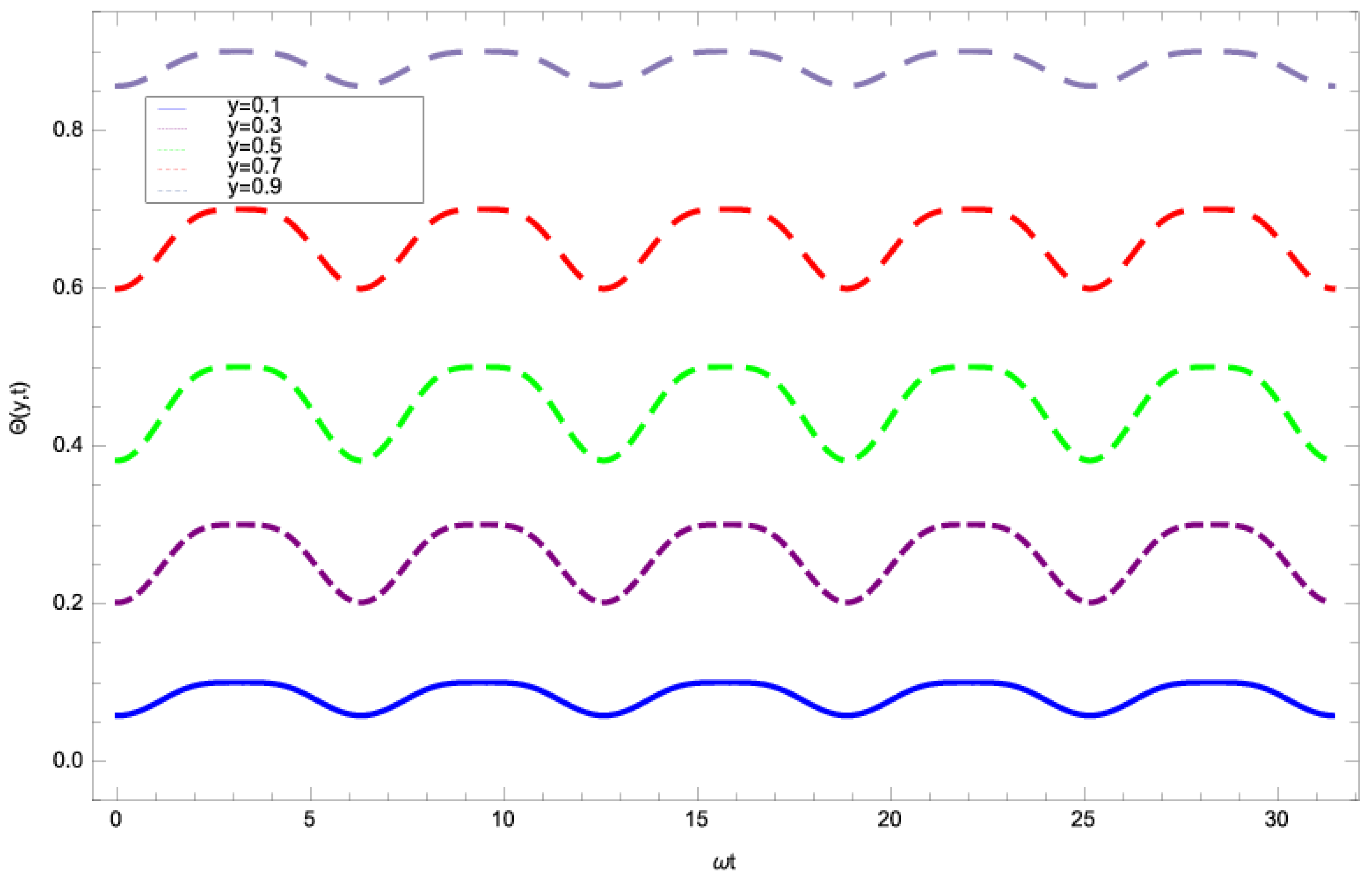
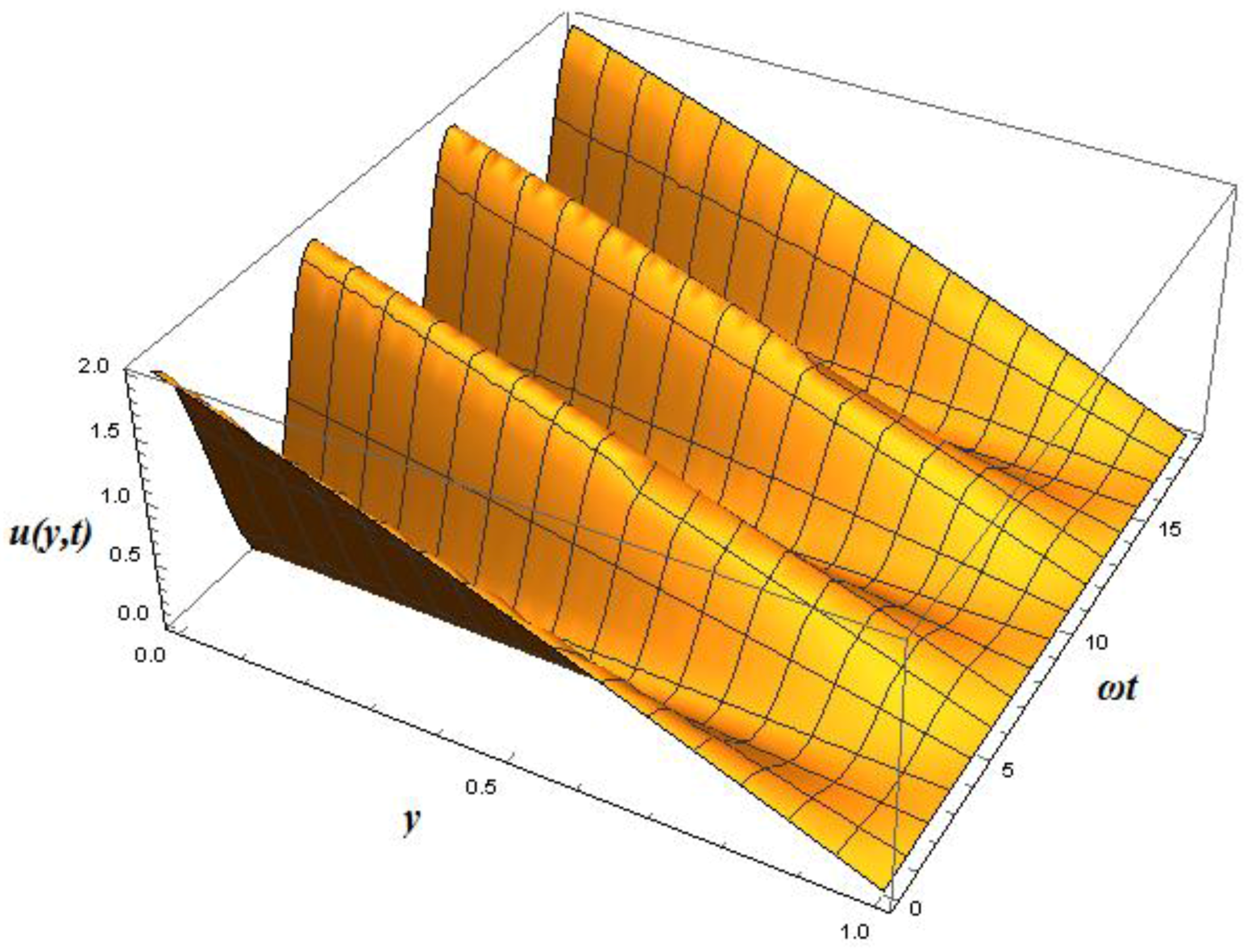
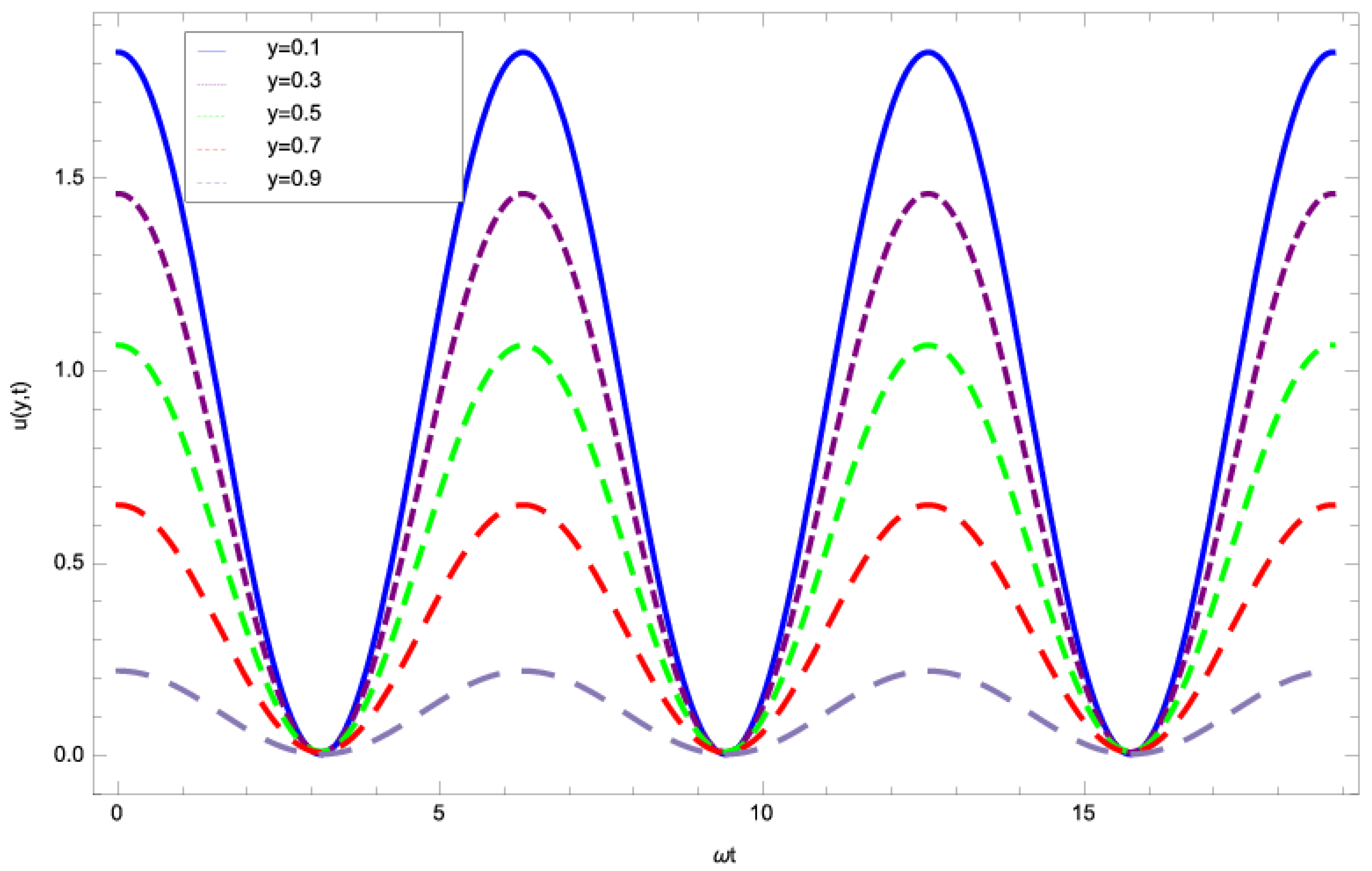
• Initially, the liquid film oscillates jointly with the plate for a selected domain $y\in [0,1]$ and this oscillation rises slowly towards the free surface.
• The gravitational effect near the belt is smaller due to the friction force, and this effect is more clear and rapid at the free surface.
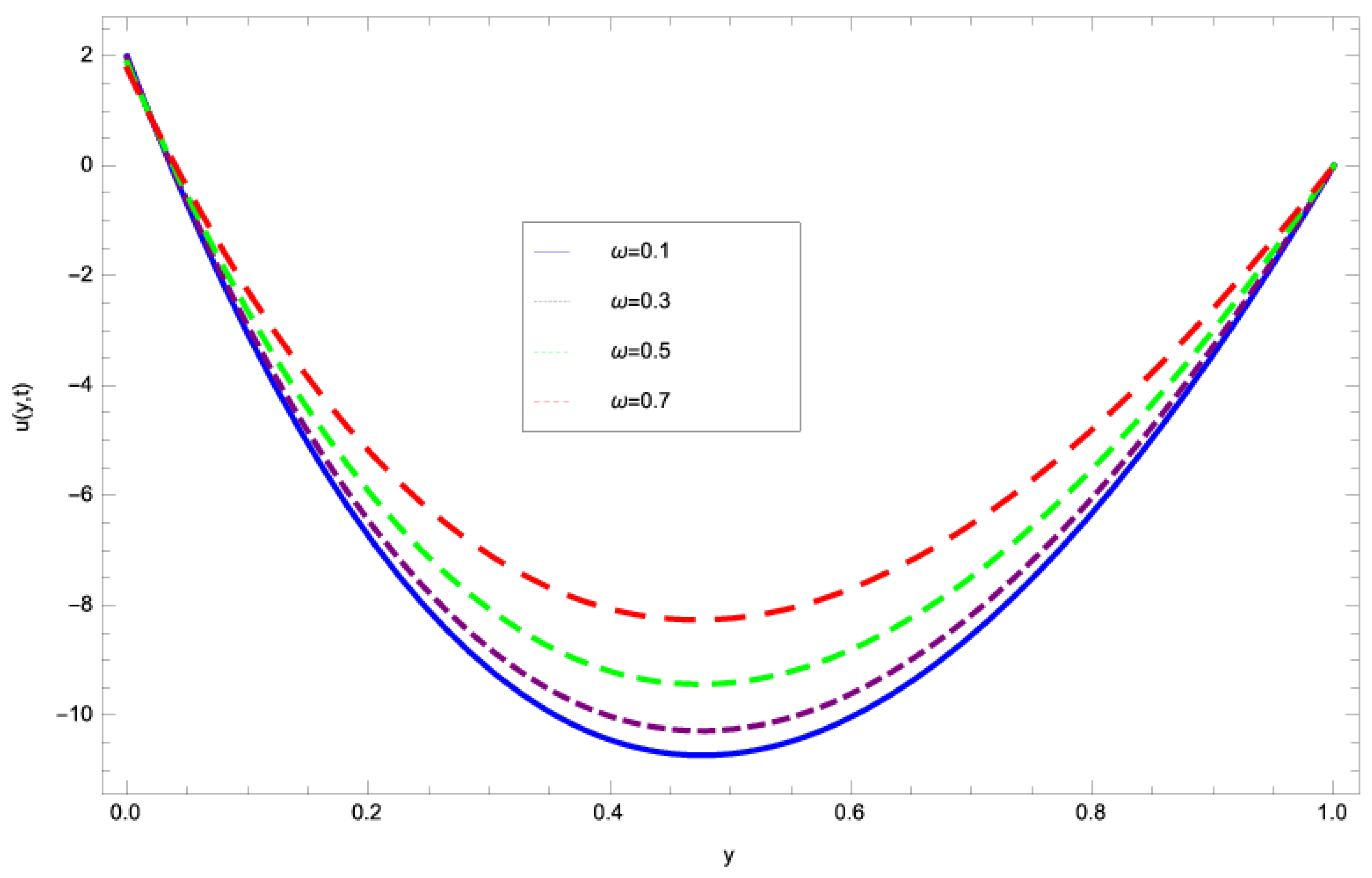
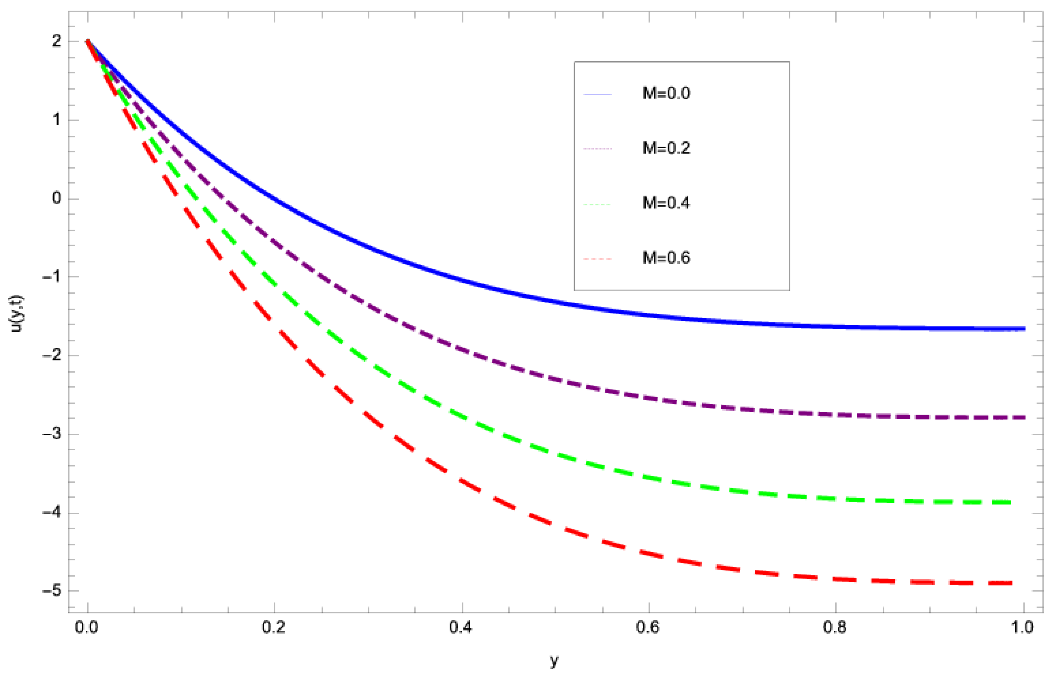
• The magnetic effect on the flow field has been observed, which opposes the fluid motion.
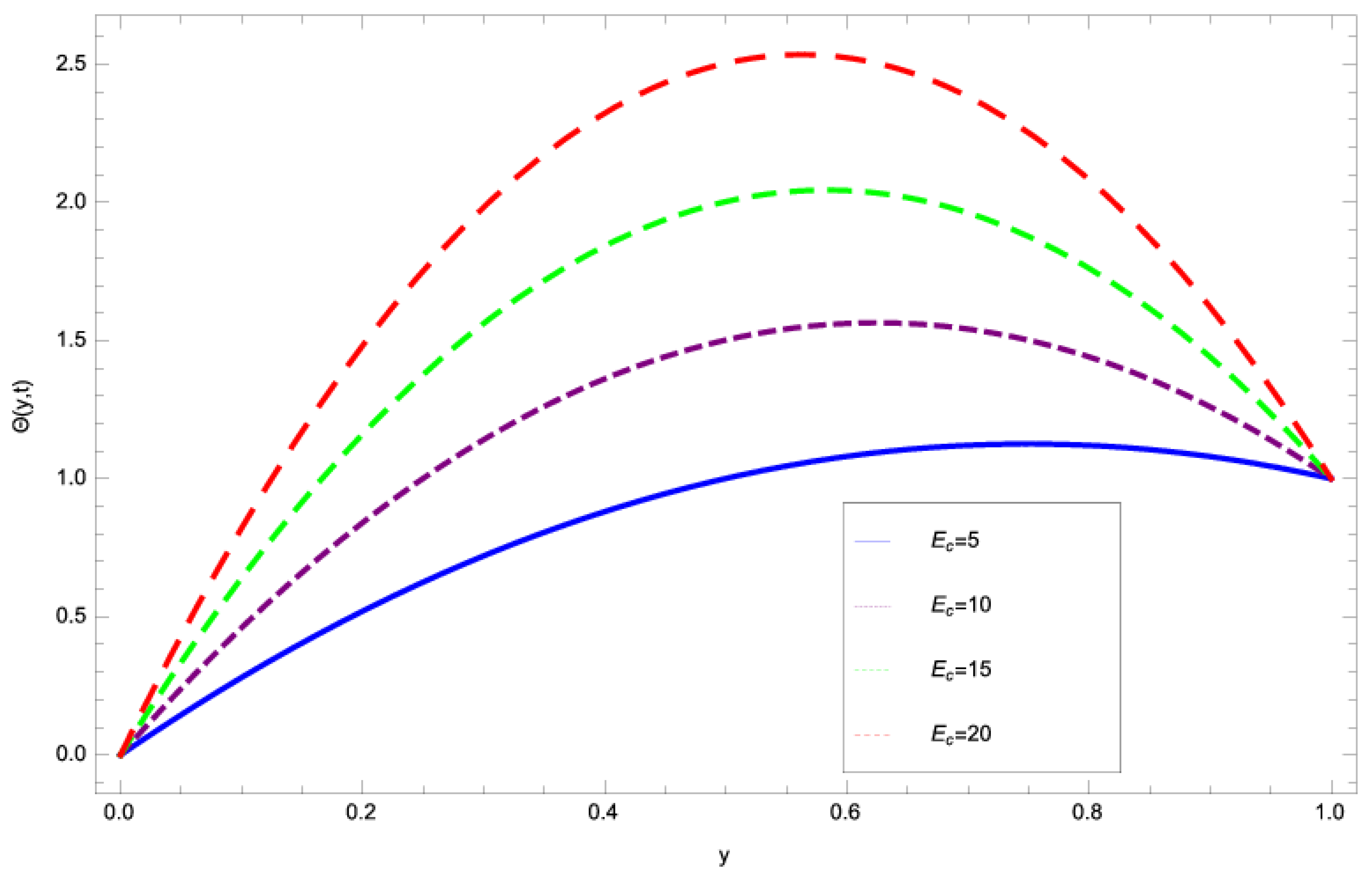
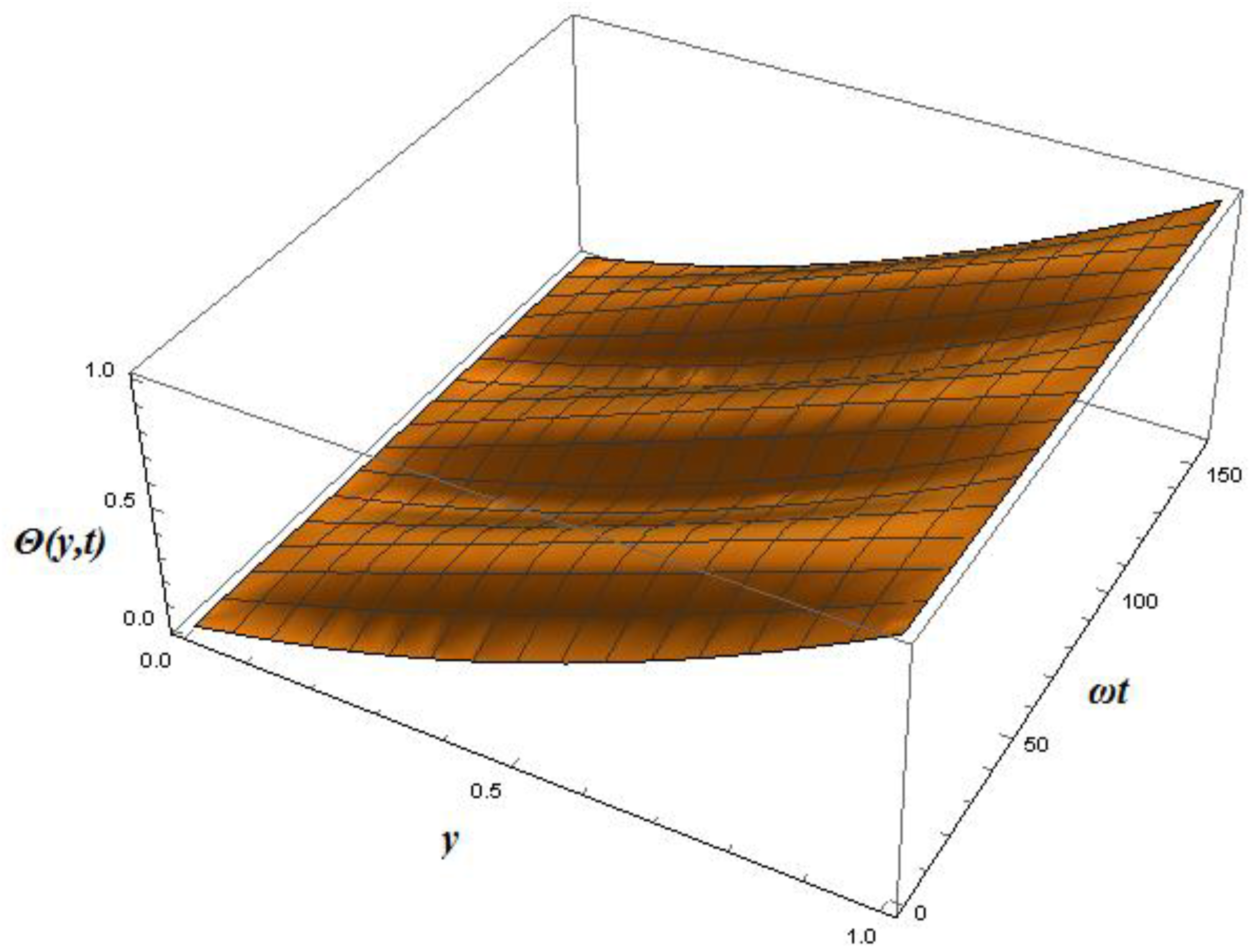
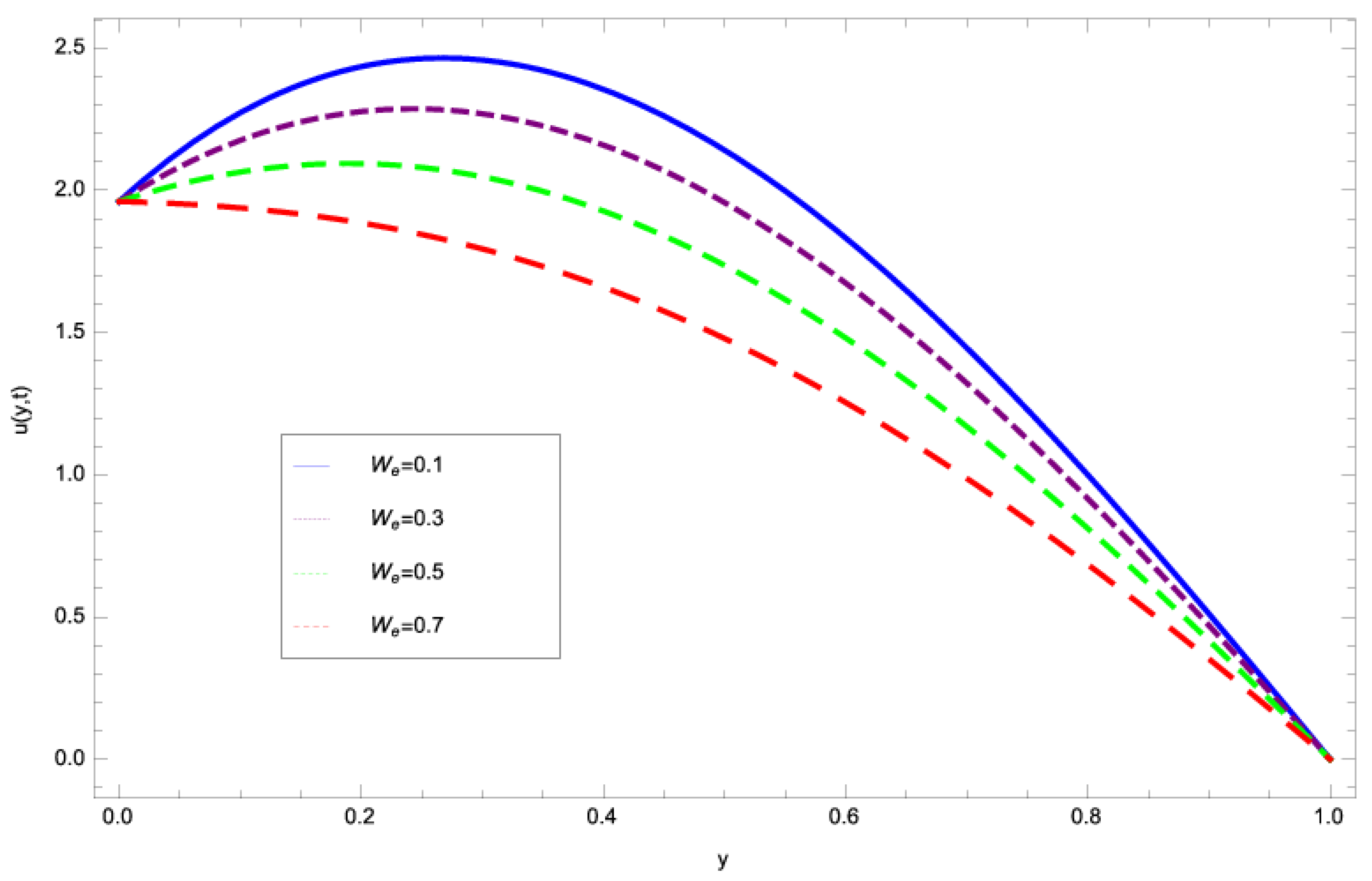
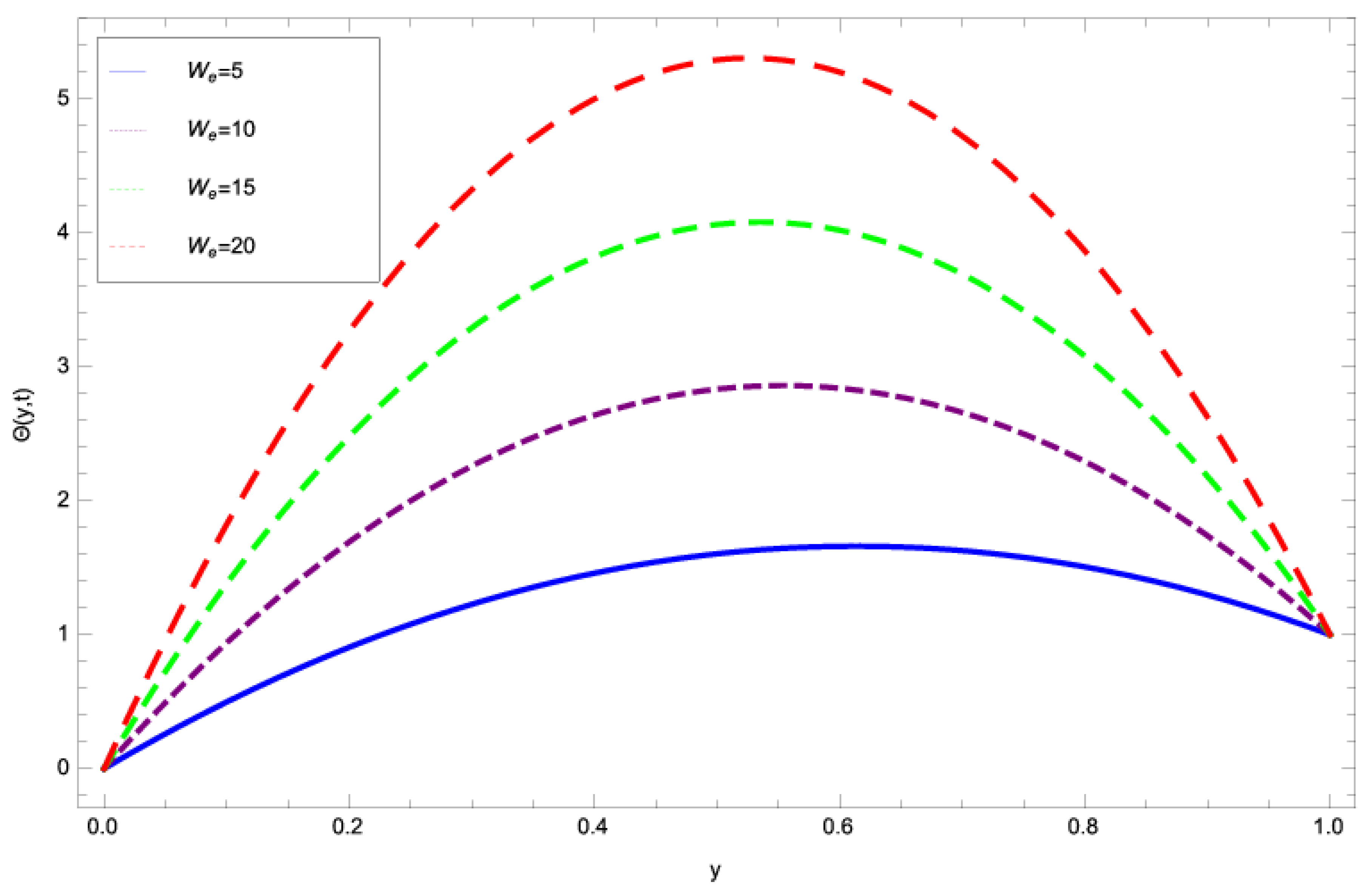
• The thermal boundary layer thickness increases with larger values of Eckert number and the inter molecular forces among the fluid particles decrease and, as a result, the velocity of fluid film increases.
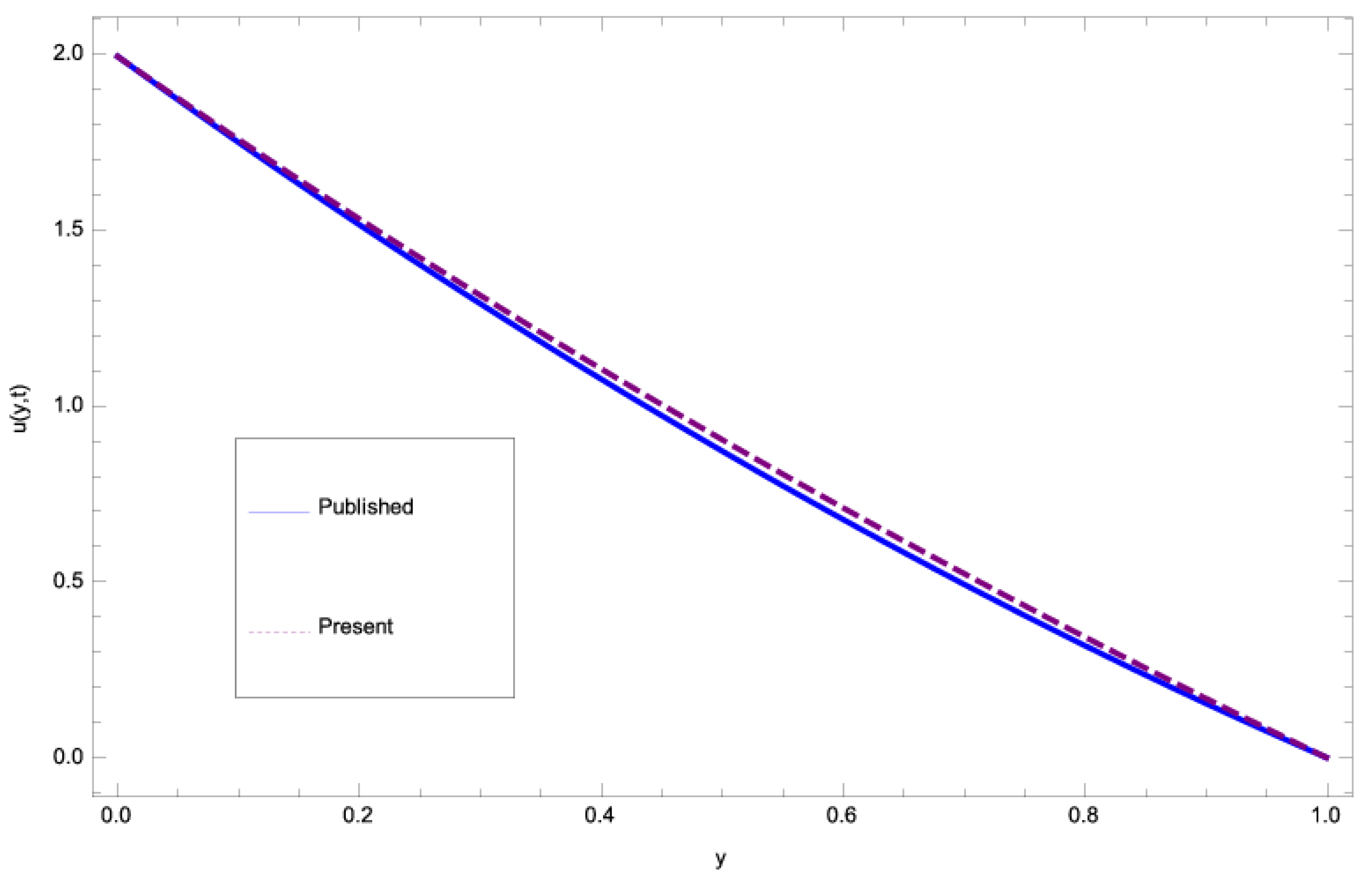
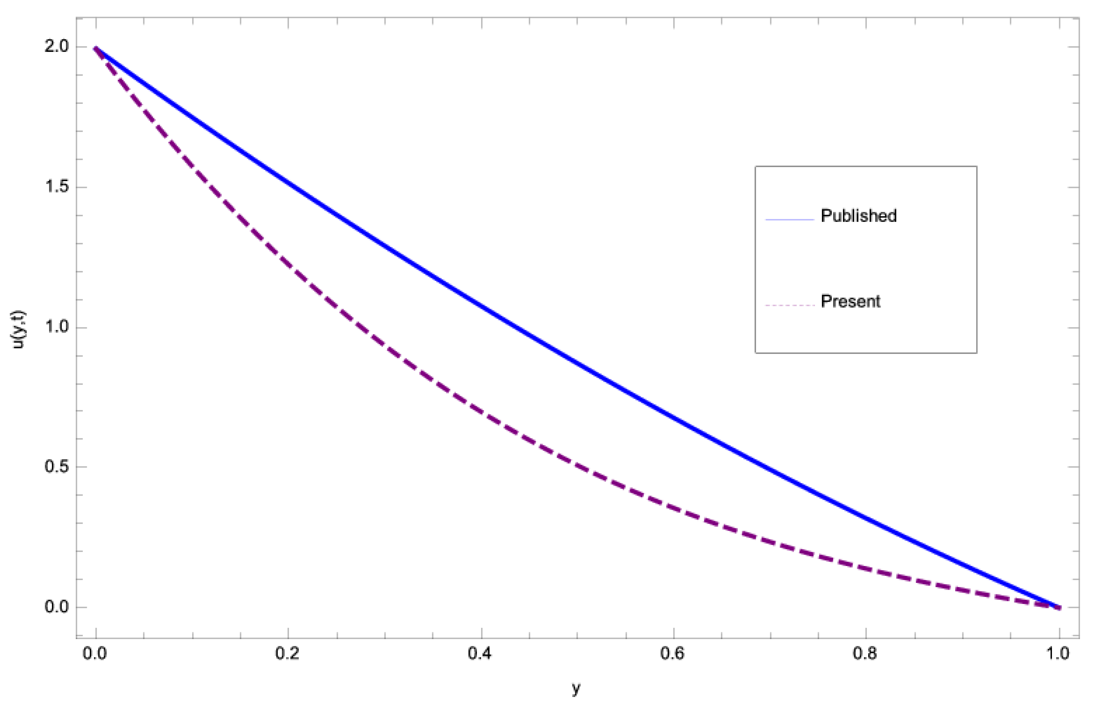
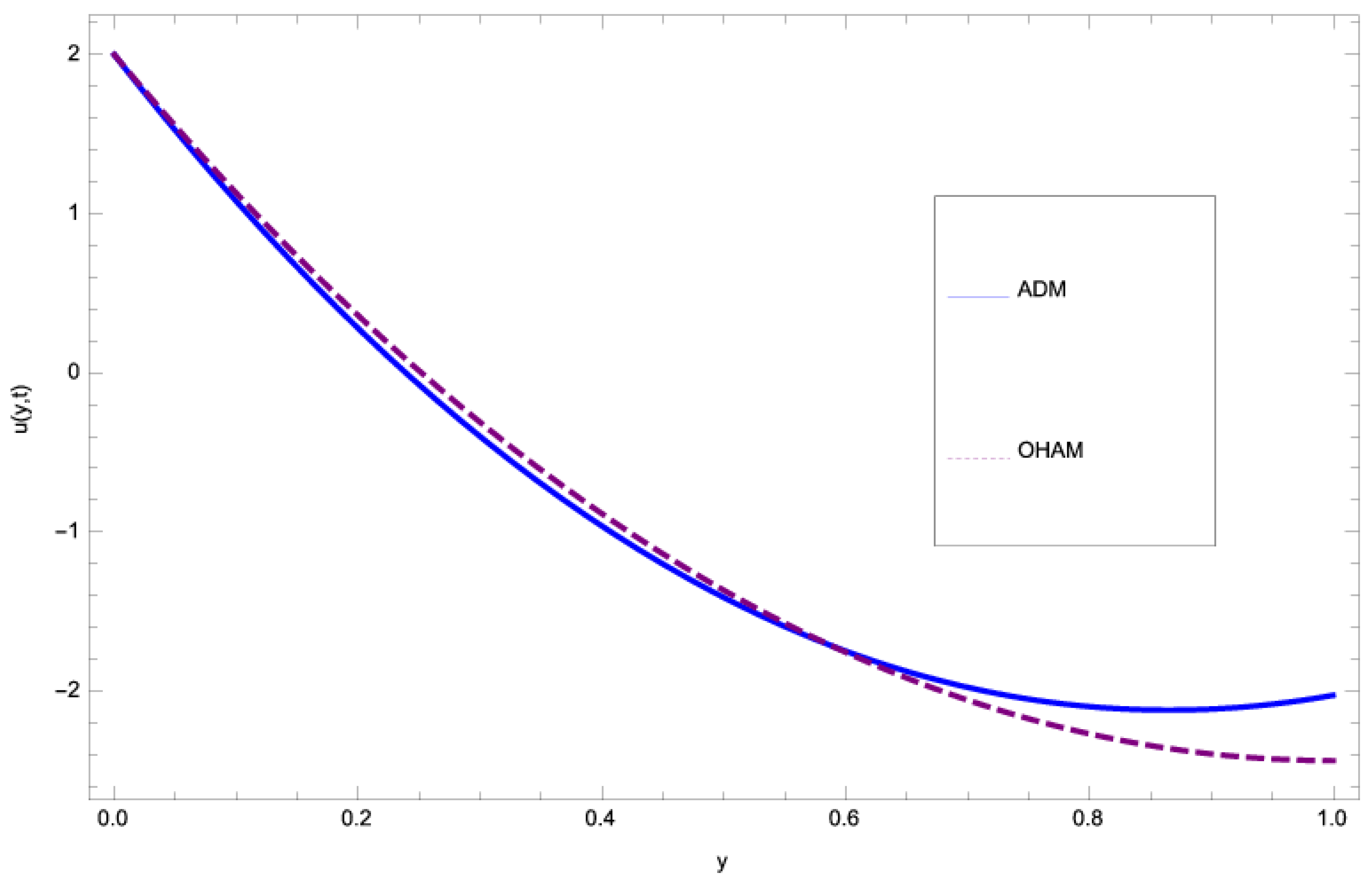
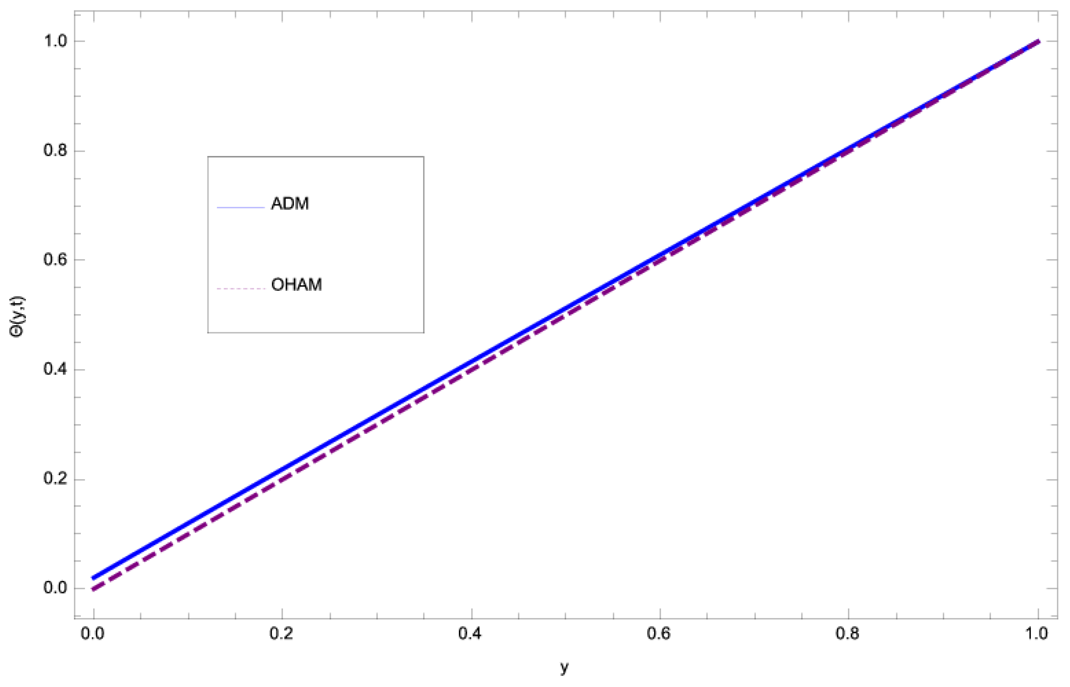
• The fast convergence of OHAM has been observed by comparing its results with ADM.

References

1. Ancey, C. Plasticity and geophysical flows: A review. J. Non-Newton. Fluid Mech. 2007, 142, 4–35. [Google Scholar] [CrossRef]
2. Griffiths, R.W. The dynamics of lava flows. Annu. Rev. Fluid Mech. 2000, 32, 477–518. [Google Scholar] [CrossRef]
3. Williamson, R.V. The flow of pseudoplastic materials. Ind. Eng. Chem. Res. 1929, 21, 1108–1111. [Google Scholar] [CrossRef]
4. Dapra, I.; Scarpi, G. Perturbation solution for pulsatile flow of a non-Newtonian Williamson fluid in a rock fracture. Int. J. Rock Mech. Min. Sci. 2006, 44, 1–8. [Google Scholar] [CrossRef]
5. Gamal, M.; Abdel, R. Unsteady magnetohydrodynamic flow of non-Newtonian fluids obeying power law model. J. Interdiscip. Math. 2007, 10, 363–368. [Google Scholar]
6. Khan, N.A.; Khan, S.; Riaz, F. Boundary Layer Flow of Williamson Fluid with Chemically Reactive Species. Math. Sci. Lett. 2014, 3, 199–205. [Google Scholar] [CrossRef]
7. Hayat, T.; Shafiq, A.; Alsaedi, A. Hydromagnetic boundary layer flow of Williamson fluid in the presence of thermal radiation and Ohmic dissipation. Alex. Eng. J. 2016, 55, 2229–2240. [Google Scholar] [CrossRef]
8. Nadeem, S.; Hussain, S.T.; Lee, C. Flow of Williamson Fluid over a Stretching Sheet. Braz. J. Chem. Eng. 2013, 30, 619–625. [Google Scholar] [CrossRef]
9. Waris, K.; Gul, T.; Idrees, M.; Islam, S.; Khan, I.; Dennis, L. Thin Film Williamson Nanofluid Flow with Varying Viscosity and Thermal Conductivity on a Time-Dependent Stretching Sheet. Appl. Sci. 2016, 6, 334. [Google Scholar]
10. Abdollahzadeh Jamalabadi, M.Y.; Hooshmand, P.; Bagheri, N.; KhakRah, H.; Dousti, M. Numerical simulation of Williamson combined natural and forced convective fluid flow between parallel vertical walls with slip effects and radiative heat transfer in a porous medium. Entropy 2016, 18, 147. [Google Scholar] [CrossRef]
11. Noor, K.; Gul, T.; Islam, S.; Khan, I.; Aisha, M.A.; Ali, S.A. Magnetohydrodynamic nanoliquid thin film sprayed on a stretching cylinder with heat transfer. Appl. Sci. 2017, 7, 271. [Google Scholar]
12. Gul, T.; Saeed, I.; Shah, R.A.; Khan, I.; Shafie, S. Thin film flow in MHD third grade fluid on a vertical belt with temperature dependent viscosity. PLoS ONE 2014, 9, 1–12. [Google Scholar] [CrossRef] [PubMed]
13. Miladinova, S.; Lebon, G.; Toshev, E. Thin Film Flow of a Power Law Liquid Falling Down an Inclined Plate. J. Non-Newton. Fluid Mech. 2014, 122, 69–70. [Google Scholar] [CrossRef]
14. Siddiqui, A.M.; Mahmood, R.; Ghori, Q.K. Homotopy perturbation method for thin film flow of a fourth grade fluid down a vertical cylinder. Phys. Lett. A 2006, 352, 404–410. [Google Scholar] [CrossRef]
15. Fetecau, C. Starting solutions for some unsteady unidirectional flows of a second grade fluid. Int. J. Eng. Sci. 2005, 43, 781–789. [Google Scholar] [CrossRef]
16. Majeed, A.; Zeeshan, A.; Ellahi, R. Unsteady Ferromagnetic Liquid Flow and Heat Transfer Analysis over a Stretching Sheet with the Effect of Dipole and Prescribed Heat Flux. J. Mol. Liquid 2016, 223, 528–533. [Google Scholar] [CrossRef]
17. Keslerova, R.; Karel, K. Numerical study of steady and unsteady flow for power-law type generalized Newtonian fluids. Computing 2013, 95, 409–424. [Google Scholar] [CrossRef]
18. Andrew, D.; Rees, S.; Andrew, P.B. Unsteady thermal boundary layer flows of a Bingham fluid in a porous medium. Int. J. Heat Mass Transf. 2015, 82, 460–467. [Google Scholar]
19. Morteza, B.N.; Maziar, C. Reduced-order modeling of three-dimensional unsteady partial cavity flows. J. Fluids Struct. 2015, 52, 1–15. [Google Scholar]
20. Fatimah, A.Z.M.S.; Jaworski, A.J. Friction factor correlation for regenerator working in a travelling-wave thermo acoustic system. Appl. Sci. 2017, 7, 253. [Google Scholar]
21. Huang, J.; Liu, M.; Jin, T. A Comprehensive Empirical Correlation for Finned Heat Exchangers with Parallel PlatesWorking in Oscillating Flow. Appl. Sci. 2017, 7, 117. [Google Scholar] [CrossRef]
22. Gul, T.; Islam, S.; Rehan, A.S.; Khan, I.; Sharidan, S. Analysis of thin film flow over a vertical oscillating belt with a second grade fluid. Eng. Sci. Technol. Int. J. 2015, 18, 207–217. [Google Scholar] [CrossRef]
23. Shah, A.R.; Islam, S.; Siddiqui, A.M.; Haroon, T. OHAM solution of unsteady second grade fluid in wire coating analysis. J. KSIAM 2011, 15, 201–222. [Google Scholar]
24. Yongqi, W.; Wei, W. Unsteady flow of a fourth-grade due to an oscillating plate. Non-Linear Mech. 2007, 42, 432–441. [Google Scholar]
25. Gul, T.; Islam, S.; Shah, R.A.; Khan, I.; Khalid, A.; Safie, S. Heat Transfer Analysis of MHD Thin Film Flow of an Unsteady Second Grade Fluid Past a Vertical Oscillating Belt. PLoS ONE 2014, 9, 1–21. [Google Scholar] [CrossRef] [PubMed]
26. Gul, T.; Islam, S.; Shah, R.A.; Khalid, A.; Khan, I.; Shafie, S. Unsteady MHD Thin Film Flow of an Oldroyd B Fluid over an Oscillating Inclined Belt. PLoS ONE 2015, 10, 1–18. [Google Scholar] [CrossRef] [PubMed]
27. Gul, T.; Fazle, G.; Islam, S.; Shah, R.A.; Khan, I.; Nasir, S.; Sharidan, S. Unsteady thin film flow of a fourth grade fluid over a vertical moving and oscillating belt. Propuls. Power Res. 2016, 5, 223–235. [Google Scholar] [CrossRef]
28. Ellahi, R.; Tariq, M.H.; Hassan, M.; Vafai, K. On boundary layer magnetic flow of nano-Ferroliquid under the influence of low oscillating over stretchable rotating disk. J. Mol. Liquids 2017, 229, 339–345. [Google Scholar] [CrossRef]
29. Sheikholeslami, M.; Ellahi, R. Electrohydrodynamic nanofluid hydrothermal treatment in an enclosure with sinusoidal upper wall. Appl. Sci. 2015, 5, 294–306. [Google Scholar] [CrossRef]
30. Sheikholeslami, M.; Zaigham Zia, Q.M.; Ellahi, R. Influence of induced magnetic field on free convection of nanofluid considering Koo-Kleinstreuer (KKL) correlation. Appl. Sci. 2016, 6, 324. [Google Scholar] [CrossRef]
31. Ellahi, R.; Hassan, M.; Zeeshan, A. Shape effects of nanosize particles in Cu-H2O nanofluid on entropy generation. Int. J. Heat Mass Transf. 2015, 81, 449–456. [Google Scholar] [CrossRef]
32. Wang, L.; Chen, X. Approximate Analytical Solutions of Time Fractional Whitham-Broer-Kaup Equations by a Residual Power Series Method. Entropy 2015, 17, 6519–6533. [Google Scholar] [CrossRef]
33. Adomian, G. Solving Frontier Problems of Physics: The Decomposition Method; Kluwer Academic Publishers: Dordrecht, The Netherlands, 1994. [Google Scholar]
34. Adomian, G. A Review of the Decomposition Method and Some Recent Results for Non-Linear Equations. Math. Comput. Model. 1992, 13, 287–299. [Google Scholar]
35. Wazwaz, A.; Adomian, M. Decomposition Method for a Reliable Treatment of the Bratu-Type Equations. Appl. Math. Comput. 2005, 166, 652–663. [Google Scholar] [CrossRef]
36. Wazwaz, A.M. Adomian Decomposition Method for a Reliable Treatment of the Emden-Fowler Equation. Appl. Math. Comput. 2005, 161, 543–560. [Google Scholar] [CrossRef]
37. Marinca, V.; Herisanu, N.; Bota, C.; Marinca, B. An optimal homotopy asymptotic method applied to the steady flow of fourth grade fluid pasta porous plate. Appl. Math. Lett. 2009, 22, 245–251. [Google Scholar] [CrossRef]
38. Marinca, V.; Herisanu, N. Application of optimal homotopy asymptotic method for solving non-linear equations arising in heat transfer. Int. Commun. Heat Mass Transf. 2008, 35, 710–715. [Google Scholar] [CrossRef]
39. Marinca, V.; Herisanu, N.; Nemes, I. Optimal homotopy asymptotic method with application to thin film flow. Cent. Eur. J. Phys. 2008, 6, 648–653. [Google Scholar] [CrossRef]
40. Mabood, F.; Khan, W.A.; Ismail, A. Optimal homotopy asymptotic method for flow and heat transfer of a viscoelastic fluid in an axisymmetric channel with a porous wall. PLoS ONE 2013, 8, 1–8. [Google Scholar] [CrossRef] [PubMed]
Figure 1. The physical configuration of the problem considering thin film flow of the Williamson fluid passing over an inclined, oscillating, and moving belt.
Applsci 07 00369 g001
Figure 2. The view of the fluid motion at time level ω t ( 0 , 6 π ) in 3D, when m = 0.3 ,   M = 0 . 2 ,   W e = 0.1   .
Applsci 07 00369 g002
Figure 3. The 3D presentation of temperature distribution at time level ω   t ( 0 , 50 π ) , when ω = 0 . 2 ,   m = 0 . 10 ,   M = 0 . 2 ,   W e = 0.1 ,   E c = 9 .
Applsci 07 00369 g003
Figure 4. The view of the fluid motion at time level ω t ( 3 π , 3 π ) in 2D, when m = 0.3 ,   M = 0 . 2 ,   W e = 0.1   .
Applsci 07 00369 g004
Figure 5. The 2D presentation of temperature distribution at time level ω t ( 4 π , 4 π ) , when ω = 0 . 2 ,   m = 0 . 10 ,   M = 0 . 2 ,   W e = 0.1 ,   E c = 9 .
Applsci 07 00369 g005
Figure 6. The magnetic effect during fluid motion, when. ω = 0 . 6 ;    m = 0.5 ;    W e = 5 ;    t = 5 .
Applsci 07 00369 g006
Figure 7. The effect of the oscillating parameter ω during fluid motion, when m = 0.5 ; W e = 5 ; M = 1.6 ; t = 1 .
Applsci 07 00369 g007
Figure 8. The effect of the Williamson number during fluid motion, when ω = 0.3 ; m = 0.5 ; M = 5 ; t = 20 .
Applsci 07 00369 g008
Figure 9. The effect of the gravitational parameter during fluid motion, when ω = 0 . 6 ;    W e = 5 ; M = 0 . 6 ;    t   = 3.5 .
Applsci 07 00369 g009
Figure 10. The effect of the Eckert number during temperature distribution, when m = 0.5 ;    W e = 5 ; M = 0 . 6 ; ω = 0.7 ; t = 1 .
Applsci 07 00369 g010
Figure 11. The effect of the Williamson number during temperature distribution, when m = 0.5 ;    E c = 8 ; M = 0.5 ; ω = 0.3 ; t = 1 .
Applsci 07 00369 g011
Figure 12. The comparison of the velocity profile of the present work and published work [18], when. α = 0.5 ; W e = 0.3 ; S t = m = 1 ; M = λ = 0 ; a = ξ = 1 ;    ω = 0.3 ; t = 0 . 6 .
Applsci 07 00369 g012
Figure 13. The comparison of the velocity profile of the present work and published work [18], when α = 0.05 ; W e = 0.03 ; S t = m = 1 ; M = λ = 0 ; a = ξ = 1 ; ω = 0.3 ; t = 0 . 6 .
Applsci 07 00369 g013
Figure 14. The comparison of Adomian Decomposition Method (ADM) and Optimal Homotopy Asymptotic Method (OHAM) methods for the velocity profile, when W e = 0.01 ,    m = 8.3 ; M = 0.01 , ω = 0.02 , t = 1 . 6 , C 1 = 1.3196149901566254 , C 2 = 0.7108355490082049 .
Applsci 07 00369 g014
Figure 15. The comparison of ADM and OHAM methods for the temperature profile, when W e = 0.1 , m = 0.01 ; M = 0.1 , ω = 0.02 , t = 0 . 6 , E c = 10 , Pr = 4 . 0 , C 1 = 0.0009350828 , C 2 = 0.0024496023 , C 3 = 2.597660913881 , C 4 = 1.59769431544815 .
Applsci 07 00369 g015