Study of the Effect of Time-Based Rate Demand Response Programs on Stochastic Day-Ahead Energy and Reserve Scheduling in Islanded Residential Microgrids

Abstract

In recent deregulated power systems, demand response (DR) has become one of the most cost-effective and efficient solutions for smoothing the load profile when the system is under stress. By participating in DR programs, customers are able to change their energy consumption habits in response to energy price changes and get incentives in return. In this paper, we study the effect of various time-based rate (TBR) programs on the stochastic day-ahead energy and reserve scheduling in residential islanded microgrids (MGs). An effective approach is presented to schedule both energy and reserve in presence of renewable energy resources (RESs) and electric vehicles (EVs). An economic model of responsive load is also proposed on the basis of elasticity factor to model the behavior of customers participating in various DR programs. A two-stage stochastic programming model is developed accordingly to minimize the expected cost of MG under different TBR programs. To verify the effectiveness and applicability of the proposed approach, a number of simulations are performed under different scenarios using real data; and the impact of TBR-DR actions on energy and reserve scheduling are studied and compared subsequently.

1. Introduction

One of the major thrust areas of demand side management (DSM) is demand response (DR) which is defined as a set of actions taken to reduce users’ electricity consumptions in response to higher market prices or market incentives [1]. Moreover, system operators may apply DR programs to reduce the load temporarily in emergency grid conditions such as unit outage or unpredictable change in renewable generation [2,3]. Therefore, the main idea of DR is to encourage customers to manage their consumption patterns in a way not only to maximize their own utility, but also to support safe operation of the power system [4].

According to the Federal Energy Regulatory Commission (FERC), DR programs can be classified into two major categories, namely, time-based rate (TBR) and incentive-based programs (IBPs) [5]. In TBR programs (also known as price-based DR programs [6]), time-varying prices are given to consumers based on the electricity price in different time periods, encouraging them to change their consumption level in response to the changing price signals. On the other hand, in IBP schemes, customers are offered fixed or time-varying incentives, to reduce their electricity consumption during periods of system stress, however they would be penalized for no participation in the program [7].

The focus of this paper is on TBR programs which are mainly divided into three categories, real-time pricing (RTP), time of use (TOU), and critical peak pricing (CPP) programs. These programs are well-suited for implementation in residential areas (e.g., residential microgrids (MGs)) where there are more possibilities for load management purposes [8,9,10,11]. However, there exist a number of challenges, such as rebound peaks during low cost periods and service interruptions. Moreover, the presence of uncertain elements within an environment such as wind and photovoltaic (PV) power generation imposes development of sophisticated balancing mechanisms between supply and demand to meet the system stability. Therefore, TBR models need to be well-designed and implemented to provide efficient operating conditions for such systems in presence of uncertainties.

Regarding the MG scheduling under uncertainty, much research has been done recently [12,13,14,15,16,17,18,19,20,21]. The effect of wind energy forecast errors on the network-constrained market-clearing problem, in which energy and reserve are simultaneously dispatched, was investigated in [12,13] using two-stage stochastic programming models. Based on the proposed method in [12], operating cost of MG was minimized with regard to the uncertainty of renewable energy resources (RESs). In [13], optimal dispatch of a MG was presented with regard to emissions and fuel consumption cost minimization using heuristic optimization. Authors in [14,15] exploited MG management as a multi-objective optimization problem to mitigate emission level as well as operation and maintenance costs. To obtain efficient energy management, artificial intelligence techniques were also used with multi-objective optimization programming [16]. However, in the reviewed literature, the procurement of the MG reserve (in terms of spinning and/or non-spinning reserve) for reliable operation of the system has been neglected. To address this issue, effective methods for providing reserve in typical MGs with high penetration of RESs are developed based on DR programs [17,18,19]. In [17], a day-ahead market structure was presented where DR can provide contingency reserves through a bidding procedure representing the cost of load curtailment. Also, authors in [18] introduced a price-responsive DR action for optimal regulation service reserve provision under high levels of wind penetration. The same type of study was carried out in [19], considering load uncertainty and generation unavailability as different working scenarios. In view of the problem-solving strategies, most of the reviewed research works have utilized stochastic programming techniques, however some have applied other methods such as robust optimization or Monte Carlo simulation [20,21]. In [22], a stochastic AC security-constrained unit commitment problem under wind power uncertainty has been formulated. Also, a stochastic multi-objective framework has been proposed in [23], for joint energy and reserve scheduling in day-ahead however, this reference has not considered AC network, load, EVs and wind power uncertainties. Furthermore, authors in [24] have proposed a multi-objective structure that can optimize objective functions including operation costs of MG, but they have not considered demand and EVs uncertainty in day-ahead scheduling.

This paper presents the effect of different types of TBR programs on the MG operation costs and shaping the load profile in presence of RESs and electrical vehicles (EVs). EVs are employed for energy scheduling or peak shaving with fast charging and discharging capabilities, while the responsive loads are used to supply a part of the required MG reserve to compensate RESs uncertainties. Monte-Carlo simulations together with k-means clustering technique are applied to create several scenarios corresponding to renewable generation variations and EVs owners’ behaviors. The generated scenarios are then reduced and fed into a two-stage optimization model developed for minimizing the operation costs. In the first stage of optimization, the energy and reserve costs are minimized simultaneously and in the second stage, the cost associated with the rescheduling of generating units (due to the variations in wind turbine (WT) and photovoltaic (PV) output powers) is minimized. Finally, simulation results for co-optimization of energy and reserves in the examined residential MG are presented and compared under different DR programs and operating conditions. As a whole, the main contributions of this paper can be highlighted as:

• Optimal management of an islanded MG with RTP-based DR programs using a scenario-based two-stage stochastic programming model.
• Simultaneous energy and reserve scheduling of MGs with regard to different DR schemes in an uncertain environment.
• Assessment of TBR-based DR programs under different scenarios with/without considering EVs participation.

The remainder of this paper is arranged as follows: a network-constrained day-ahead market clearing model is introduced in Section 2 and it is reformulated into a mixed integer programming (MIP) model in Section 3. The case studies are presented in Section 4 and the simulation results are discussed thereafter. Finally, Section 5 concludes this paper with future scope.

2. Model Description

A network-constrained day-ahead market clearing model is developed under a two-stage stochastic programming framework in order to accommodate the uncertain nature of RESs and EVs. Based on [25] the MG uncertainties can be categorized into two groups:

(1)

Normal operation uncertainties (including errors in forecasting wind data, EV operation, and real-time market prices).

(2)

Contingency-based uncertainties (including random forced outages, unintentional islanding, and resynchronization events).

The subject area of this paper mainly falls in the first category so the optimization model is developed in a way to effectively consider normal operation uncertainties including forecasting errors of WT and PV power production and EV owner behaviors. A set of scenarios representing MG uncertainties are generated for scheduling horizon. In order to render the problem tractable, an appropriate scenario-reduction algorithm is applied to reduce the generated scenarios into an optimal subset that represents well enough the uncertainties. In the next step, the optimization problem is solved in two stages using commercially-available software packages. In the first stage of the proposed optimization model, energy and reserves are jointly scheduled to balance supply and demand. The second stage corresponds to operation management in several actual MG modes and deals with variables that are scenario-dependent and have different values for every single scenario. In other words, the first stage corresponds to the optimal decision for the deterministic base case, while the second stage examines the feasibility and optimality of the first stage decisions under system contingencies.

In the proposed framework, different customers sign contracts for participating in various TBR programs and submit them to the MG operator. Based on the type of the consumers’ contributions, MG operator finds the optimal day-ahead energy and reserve scheduling with regard to the minimum expected cost of operation. At the same time, optimum participation level of consumers in each DR program for reserve procurement is determined. Also, MG operator schedules the charging and discharging process of the EVs for any time intervals in the studied period.

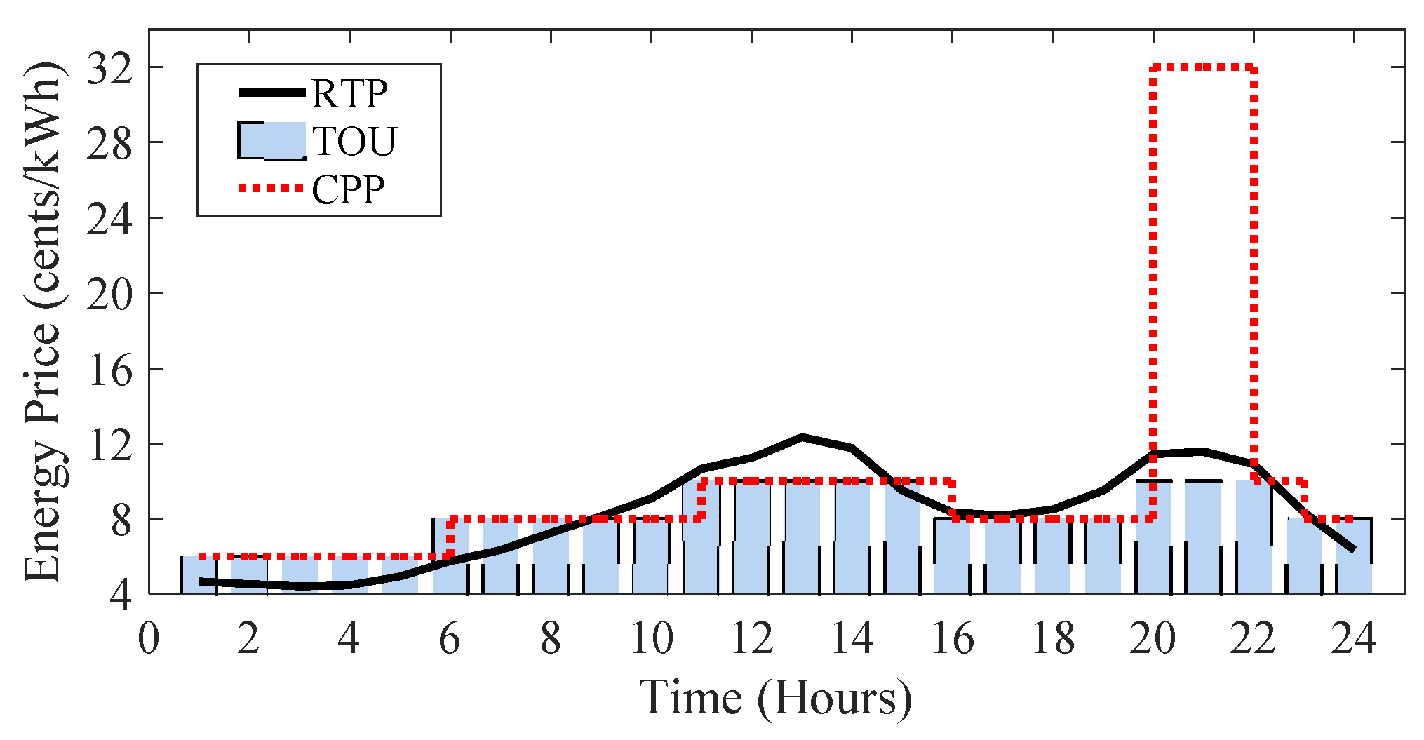
2.1. Market-Based DR Model

In order to evaluate the impact of residential customers’ participation in DR programs on load profile characteristics, an economic model of responsive loads is developed on the basis of elasticity factors. Elasticity is defined as demand sensitivity with respect to the electricity prices [26].

$$E(t,t)=\frac{{\rho }_0(t)}{D(t)}\frac{\partial D(t)}{\partial \rho (t)}$$

(1)

where, $D(t)$ and ${\rho }_0(t)$ are the nominal/initial value of demand and electricity price, respectively. Based on a single-period elastic load model, the customer changes his demand to achieve the maximum benefit from $D(t)$ to $D_{DR}(t)$ as:

$$D_{DR}(t)=D(t)+\Delta D(t)$$

(2)

The customer benefit for the tth time interval can be calculated as:

$$S(D_{DR}(t))=B(D_{DR}(t))-D_{DR}(t)\cdot \rho (t)$$

(3)

where, $S(D_{DR}(t))$ and $B(D_{DR}(t))$ represent customer benefit and income at time $t$ after implementing DR programs, respectively. In order to maximize customer benefit, the following condition must be met [27]:

$$\frac{\partial S(D_{DR}(t))}{\partial D_{DR}(t)}=0\Rightarrow \frac{\partial B(D_{DR}(t))}{\partial D_{DR}(t)}=\rho (t)$$

(4)

Therefore, the customer utility function would get a quadratic form as follows [27]:

$$B(D_{DR}(t))=B_0(t)+{\rho }_0(t)[D_{DR}(t)-D(t)]\times \left[1+\frac{D_{DR}(t)-D(t)}{2E(t,t)\cdot D(t)}\right]$$

(5)

Differentiating (5) with respect to $D_{DR}(t)$ and substituting the result in (4) yields:

$$\rho (t)={\rho }_0(t)·\left[1+\frac{D_{DR}(t)-D(t)}{E(t,t)\cdot D(t)}\right]$$

(6)

Therefore, a customer’s consumption behavior over the time can be obtained as follows:

$$D_{DR}(t)=D(t)\cdot \left[1+E(t,t)\cdot \frac{\rho (t)-{\rho }_0(t)}{{\rho }_0(t)}\right]$$

(7)

In a multi-period elastic loads model, the price elasticity of the tth period versus the hth period can be defined as [26]:

$$E(t,h)=\frac{{\rho }_0(h)}{D_0(t)}\cdot \frac{\partial D(t)}{\partial \rho (h)}$$

(8)

Considering the linear relationship between the hourly demand level and the electricity prices, it can be expressed that:

$$D_{DR}(t)=D(t)\cdot \left[1+{\displaystyle \sum _{\begin{array}{l}t=1\\ t\ne h\end{array}}^{T}E(t,h)}\cdot \frac{\rho (h)-{\rho }_0(h)}{{\rho }_0(h)}\right]$$

(9)

Combining (7) and (9), the responsive load economic model can be extracted as follows:

$$D_{DR}(t)=D(t)\cdot [1+E(t,t)\cdot \frac{\rho (t)-{\rho }_0(t)}{{\rho }_0(t)}+{\displaystyle \sum _{\begin{array}{l}h=1\\ h\ne t\end{array}}^{T}E(t,h)}\cdot \frac{\rho (h)-{\rho }_0(h)}{{\rho }_0(h)}]$$

(10)

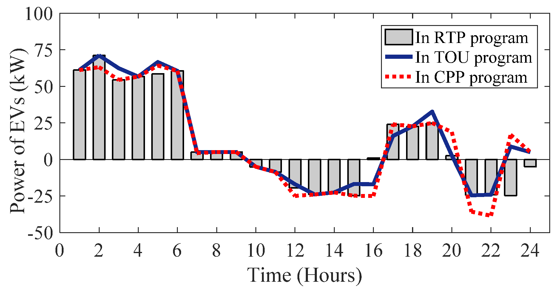
2.2. EVs Participation in DR Programs

EVs can be considered in three different modes: grid-connected mode, idle mode, or driving mode. In grid-connected mode, the MG operator can schedule charging/discharging process of EVs batteries. EVs can exchange power with the MG based on their state of charge (SOC), stop time in the parking lot (PL) and the electricity price in each DR program. In this case, EVs are considered to be probabilistic loads or generations which can be evaluated by stochastic methods [28]. The exchange power between each EV and the network can be obtained as [28]:

$$P_{k,t}^{EV}={\eta }_c{P}_{k,t}^c-\frac{P_{k,t}^d}{{\eta }_d}\hspace{1em}\hspace{1em}\begin{array}{c}\forall t\in u_k\end{array}$$

(11)

The SOC of EVs connected to the network is updated by Equation (12) [28].

$$B{C}_k\cdot SO{C}_{k,t}=B{C}_k\cdot SO{C}_{k,t-1}+P_{k,t-1}^{EV}\hspace{1em}\hspace{1em}\forall t\in {\rm T},\forall k\in Nk$$

(12)

where $SO{C}_{k,t-1}=SO{C}_{k,I}$, if $t=1$. $B{C}_k$ is battery capacity of EV in kWh and $SO{C}_{k,I}$ is the initial SOC of kth EV. It is important to control the charge and discharge energy of the parked vehicle w such that the SOC of the battery could be kept within the allowed range $SO{C}_k^{\min }$ and $SO{C}_k^{\max }$.

Besides, in idle or driving mode, there is no power exchange between EV and the network, however the stored energy might decrease depending on the EV trip length ($L_k$) and its energy consumption rate ($r_k$). It is assumed that each EV returns to the PL after driving $L_k$ km and is plugged back into the network. Thus, the SOC at the time of arrival ($SO{C}_k^{ent}$) can be estimated by Equation (13) [28].

$$SO{C}_k^{ent}=SO{C}_k^{\mathrm{int}}-L_k\times r_k\hspace{1em}\hspace{1em}\forall k\in Nk$$

(13)

where, $SO{C}_k^{\mathrm{int}}$ is the initial SOC at the beginning of the trip.

2.3. Renewable Energy Resources

Output power of WT and PV plants are inherently intermittent. In order to model the stochastic wind speed (and the WT behavior accordingly), the divided Weibull probability density function (PDF) is usually employed. The general Weibull PDF of wind speed can be formulated as follows [29]:

$$PDF(v)=\frac{k}{c}{(\frac{v}{c})}^{k-1}\cdot e^{-{(\frac{v}{c})}^k}$$

(14)

where $v$, $k$ and $c$ are wind speed, shape factor (dimensionless) and scale factor, respectively.

Besides, the output power of WT can be described by Equation (15) [30]:

$$P_w(v)=P_w^r\cdot \{\begin{array}{ll}0& ;0\le v\le v_{in}\hspace{1em}and\hspace{1em}v\ge v_{out}\\ \frac{v_{in}^3}{v_{in}^3-v_r^3}+\frac{b{v}^3}{v_r^3-v_{in}^3}& ;v_{in}\le v\le v_r\\ 1& ;v_r\le v\le v_{out}\end{array}$$

(15)

where $v_r$, $v_{in}$ and $v_{out}$ indicate the rated speed, cut-in speed and cut-out speed of the WT, respectively, and $P_w^r$ represents the total rated power of WT.

The distribution of hourly irradiance usually follows a bimodal distribution, which can be seen as a linear combination of two unimodal distribution functions [31,32]. A Beta PDF is utilized for each unimodal, as stated in the following [31]:

$$f_b(\phi )=\{\begin{array}{l}\frac{\mathrm{\Gamma }(\alpha +\beta )}{\mathrm{\Gamma }(\alpha )\cdot \mathrm{\Gamma }(\beta )}\cdot {\phi }^{(\alpha -1)}\times {(1-\phi )}^{\beta -1}\begin{array}{cc}for& \begin{array}{c}0\le \phi \le 1,\alpha \ge 0,\beta \ge 0\end{array}\end{array}\\ 0\hspace{1em}\hspace{1em}\hspace{1em}\hspace{1em}\hspace{1em}\hspace{1em}\hspace{1em}\hspace{1em}\hspace{1em}\begin{array}{c}\begin{array}{cc}& otherwise\end{array}\end{array}\end{array}$$

(16)

The parameters of the Beta distribution function ($\alpha$, $\beta$) are calculated based on the mean ($\mu$) and standard deviation ($\sigma$) of the random variable [31].

In this paper, to model the uncertainties of output power for WT and PV units, a set of possible scenarios is generated based on Metropolis–Hastings algorithm and reduced thereafter to a number of distinct scenarios using the k-means clustering technique [33].

3. Optimization Problem Formulation

3.1. Objective Function

The objective function is defined based on the minimization of the total expected cost (EC) of an isolated residential MG which includes cost of energy and reserve provision as well as the operating cost in different working scenarios.

$$\begin{array}{ll}EC& ={\displaystyle \sum _{t=1}^T{\displaystyle \sum _{i=1}^{Ng}[(A_i\cdot u_{i,t}+B_i\cdot P_{i,t})+SU{C}_i\cdot y_{i,t}+SD{C}_i\cdot z_{i,t}}}\\ & \begin{array}{c}+(C_{i,t}^{R^D}\cdot R_{i,t}^D+C_{i,t}^{R^U}\cdot R_{i,t}^U+C_{i,t}^{R^{NS}}\cdot R_{i,t}^{NS})]\end{array}\\ & +{\displaystyle \sum _{w=1}^{Nw}{C}_{w,t}\cdot P_{w,t}}+{\displaystyle \sum _{p=1}^{Np}{C}_{p,t}\cdot P_{p,t}}\\ & +{\displaystyle \sum _{k=1}^{N{k}_d}SP{R}_t\cdot P_{k,t}^d}-{\displaystyle \sum _{k=1}^{N{k}_c}BP{R}_t\cdot P_{k,t}^c}\\ & +{\displaystyle \sum _{t=1}^T{\displaystyle \sum _{j=1}^{Nj}{C}_{j,t}^{R^D}\cdot R_{j,t}^D+C_{j,t}^{R^U}\cdot R_{j,t}^U}}-{\displaystyle \sum _{j=1}^{Nj}{C}_{j,t}\cdot L_{j,t}}\\ & +{\displaystyle \sum _{s=1}^{Ns}{\displaystyle \sum _{t=1}^T{\displaystyle \sum _{i=1}^{Ng}[SU{C}_i\cdot (y_{i,t,s}-y_{i,t})+SD{C}_i\cdot (z_{i,t,s}-z_{i,t})}}}\\ & \begin{array}{c}+C_{i,t}\cdot (r_{i,t,s}^U+r_{i,t,s}^{NS}-r_{i,t,s}^D)]\end{array}\\ & +{\displaystyle \sum _{s=1}^{Ns}{\displaystyle \sum _{t=1}^T[{\displaystyle \sum _{j=1}^{Nj}{C}_{j,t}\cdot (r_{j,t,s}^U-r_{j,t,s}^D)}}}\\ & \begin{array}{c}+{\displaystyle \sum _{w=1}^{Nw}{C}_{w,t}\cdot \Delta P_{w,t,s}}+{\displaystyle \sum _p^{Np}{C}_{p,t}\cdot \Delta P_{p,t,s}}]\end{array}\\ & +{\displaystyle \sum _{j=1}^{Nj}{V}^{LOL}\cdot L_{j,t,s}^{shed}}\end{array}$$

(17)

In Equation (17), the first line of the objective function states the costs associated with energy provided from the generating units and the start-up and shut-down costs, and the second line expresses the commitment of the generating units to provide reserves. The third line denotes the costs associated with energy provided from the WT and PV units. The fourth line expresses the cost associated with charge/discharge of EVs and the fifth line considers the utility of the demand loads and their up and down reserve provision.

The rest of the terms in the objective function deal with the operating cost in different working scenarios. In this regard, the sixth and the seventh lines consider cost of unit commitment and the cost of deploying reserves from those units in different scenarios. The eighth line represents the cost of deploying reserves from DR programs and the ninth line states the costs associated with energy provided from WT and PV units. Here, it is assumed that the MG operator would pay for energy provided by WT and PV. Finally, the last term stands for the expected cost of energy not served for the inelastic loads.

3.2. Constraints

The problem constraints include two parts; the first-stage constraints and second-stage constraints. The first-stage ones are associated with the base case scenario (i.e., deterministic operating condition), and can be expressed as follows:

• Power balance in steady state; Equation (18) represents the active power balance in MG in steady state [21].

  $${\displaystyle \sum _{i=1}^{Ngb}{P}_{i,t}}+{\displaystyle \sum _{w=1}^{Nwb}{P}_{w,t}}+{\displaystyle \sum _{p=1}^{Np}{P}_{p,t}}+{\displaystyle \sum _{k=1}^{Nk{b}_d}{P}_{k,t}^d}=L_{b,t}+{\displaystyle \sum _{k=1}^{Nk{b}_c}{P}_{k,t}^c+}{\displaystyle \sum _{l=1}^{Lb}{F}_{l,t}}\hspace{1em}\hspace{1em}\forall b,\forall t$$

  (18)

  where, $F_{l,t}$ is power flow through line l in period t, ($F_{l,t}=\frac{1}{X_l}({\delta }_{ls}-{\delta }_{lr})$), ${\delta }_{x,t}$ is voltage angle at node x in period t. The power flow through line l is limited as:

  $$-F_{l,t}^{\min }\le F_{l,t}\le F_{l,t}^{\max }\hspace{1em}\hspace{1em}\forall l,\forall t$$

  (19)
• Real power generation constraints; The real power generated by DG units are constrained by (20) and (21) [21].

  $$P_{i,t}\le P_i^{\max }{u}_{i,t}-R_{i,t}^U\hspace{1em}\hspace{1em}\forall i,\forall t$$

  (20)

  $$P_{i,t}\ge P_i^{\min }{u}_{i,t}+R_{i,t}^D\hspace{1em}\hspace{1em}\forall i,\forall t$$

  (21)
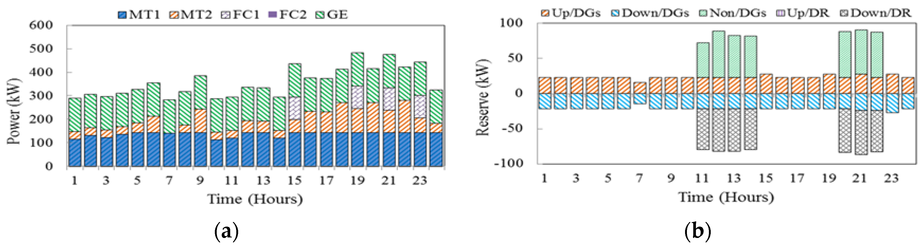
• Generation-side reserve limits; Constraints (22)–(24) impose limits on the provision of spinning reserve in terms of up and down regulations, as well as non-spinning reserve from the generating units.

  $$0\le R_{i,t}^U\le R_{i,t}^{U,\max }{u}_{i,t}\hspace{1em}\hspace{1em}\forall i,\forall t$$

  (22)

  $$0\le R_{i,t}^D\le R_{i,t}^{D,\max }{u}_{i,t}\hspace{1em}\hspace{1em}\forall i,\forall t$$

  (23)

  $$0\le R_{i,t}^{NS}\le R_{i,t}^{NS,\max }(1-u_{i,t})\hspace{1em}\hspace{1em}\forall i,\forall t$$

  (24)
• Demand-side reserve limits; Constraints (25) and (26) restrict the procurement of up and down reserves from the responsive loads.

  $$0\le R_{j,t}^U\le R_{j,t}^{U,\max }\hspace{1em}\hspace{1em}\forall j,\forall t$$

  (25)

  $$0\le R_{j,t}^D\le R_{j,t}^{D,\max }\hspace{1em}\hspace{1em}\forall j,\forall t$$

  (26)
• Unit commitment constraints; Equation (27) determines the start-up and shut-down status of units, while (28) states that a unit cannot start-up and shut-down during the same period [29].

  $$y_{i,t}-z_{i,t}=u_{i,t}-u_{i,t-1}\hspace{1em}\hspace{1em}\forall i,\forall t$$

  (27)

  $$y_{i,t}+z_{i,t}-1\le 0\hspace{1em}\hspace{1em}\forall i,\forall t$$

  (28)
• Generating units startup cost constraint; constraints (29) and (30) represent generating units startup cost limitations [21].

  $$SU{C}_{i,t}\ge {\lambda }_{i,t}^{SU}(u_{i,t}-u_{i,t-1})\hspace{1em}\hspace{1em}\forall i,\forall t$$

  (29)

  $$SU{C}_{i,t}\ge 0\hspace{1em}\hspace{1em}\forall i,\forall t$$

  (30)

The second-stage constraints account for stochastic operating conditions are the same as the first-stage constraints and mentioned in Appendix A.

4. Simulation Results and Discussion

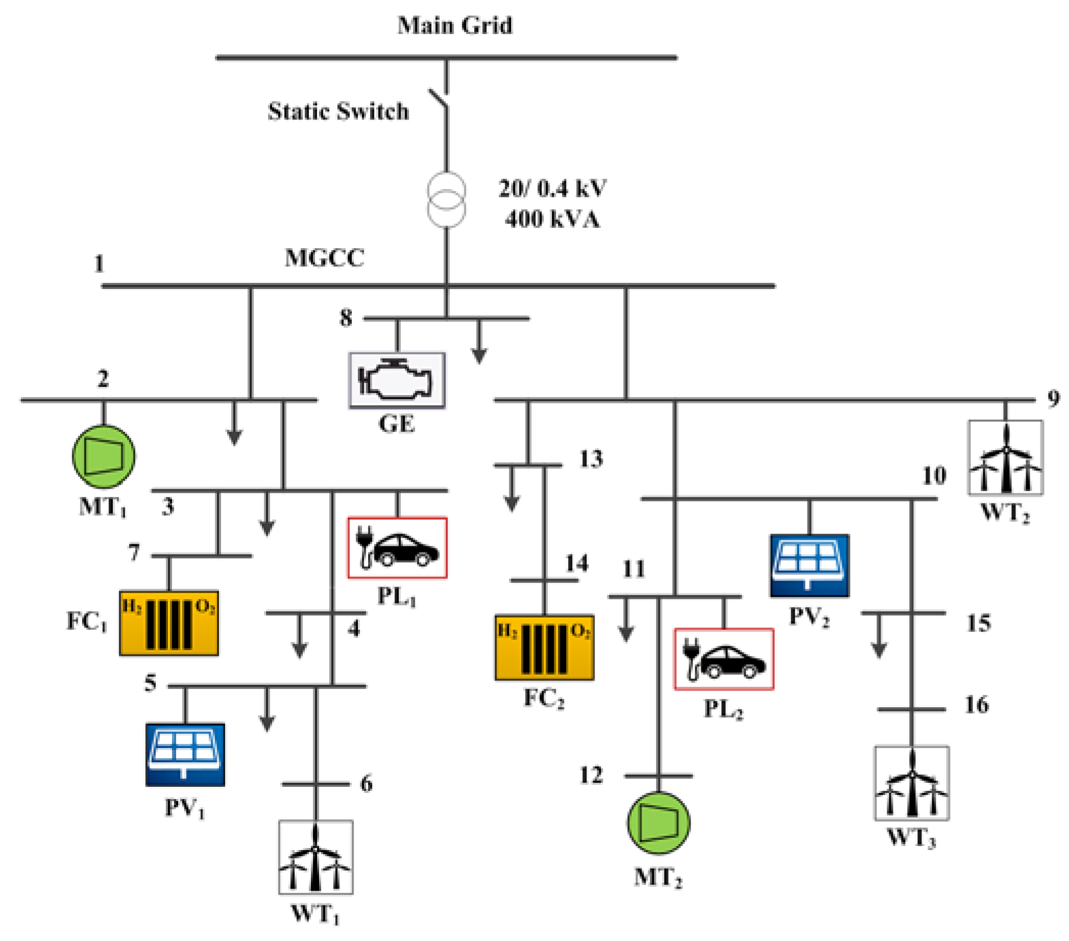
4.1. Test Case

The simulations are performed over a modified residential MG which is presented in Figure 1 [30]. There are different types of distributed generation (DG) units in the MG including two micro-turbines (MT₁ & MT₂), two fuel cell (FC₁ & FC₂) units, and one gas engine (GE) unit. Also, there are a number of renewable-based prime movers in the system including three WTs, each with a capacity of 80 kW installed at bus 6, 9 and 16, respectively and two PV plants, each with a capacity of 70 kW installed at buses 5 and 10, respectively. The wind and PV power generation are a function of random wind speed and sun radiation, respectively. Their output power scenarios are reduced by applying a k-means algorithm as shown in Figure 2. Technical specifications of the simulated MG components are given in

Table 1. Technical specifications of the simulated microgrid (MG) components.

Emission (kg/kWh)	${\mathit{C}}^{{\mathit{R}}^{\mathit{N}\mathit{S}}}$ ($)	${\mathit{C}}^{{\mathit{R}}^{\mathit{D}}}$ ($)	${\mathit{C}}^{{\mathit{R}}^{\mathit{U}}}$ ($)	SDC ($)	SUC ($)	B ($)	A ($/kWh)	${\mathit{P}}^{\mathbf{max}}$ (kW)	${\mathit{P}}^{\mathbf{min}}$ (kW)	DG
0.550	0.019	0.020	0.021	0.080	0.090	0.043	0.851	150	25	MT1
0.550	0.019	0.020	0.021	0.080	0.090	0.044	0.851	150	25	MT2
0.377	0.015	0.015	0.015	0.090	0.160	0.028	2.552	100	20	FC1
0.377	0.015	0.015	0.015	0.090	0.160	0.029	2.552	100	20	FC2
0.890	0.017	0.017	0.017	0.080	0.120	0.031	2.120	150	35	GE
-	-	-	-	-	-	0.106	0	80	0	WT
-	-	-	-	-	-	0.548	0	70	0	PV

[34]. Moreover, the hourly load profile of the MG is illustrated in Figure 3 and is supposed to be divided into three different periods, namely valley period (00:00–5:00), off-peak periods (5:00–10:00, 16:00–19:00 and 22:00–24:00) and peak periods (11:00–15:00 and 20:00–22:00).

In this study, it is assumed that the total signed contracts for participating customers in DR programs are equal to 40% of the total load during the scheduling period. The price elasticity of demand is shown in

Table 2. Price elasticity of demand.

23–24	20–22	16–19	11–15	6–10	1–5	Hour
0.03	0.034	0.03	0.034	0.03	−0.08	1–5
0.03	0.04	0.03	0.04	−0.11	0.3	6–10
0.04	0.01	0.04	−0.19	0.04	0.034	11–15
0.03	0.04	−0.11	0.04	0.03	0.03	16–19
0.04	−0.19	0.03	0.01	0.04	0.034	20–22
−0.11	0.04	0.03	0.04	0.03	0.03	23–24

, which is adopted from [27] with some modification. It is also assumed that there are two PLs with 40 charging stations in buses 3 and 11. The arrival time of EVs is modeled with a Gaussian distribution with $\mu$ = 19 and ${\delta }^2$ = 10 [35]. Moreover, the EVs connected to the MG are assumed to be capable of providing slow, medium and fast charging modes [28,36]. For the studied MG, energy prices at different tariffs (RTP, TOU and CPP) are also depicted in Figure 4.

The optimization horizon is considered to be a day with 24 time intervals. To simulate the environmental/behavioral uncertainties within the system, 3000 scenarios are generated based on Weibull, Beta, and Gaussian PDFs to represent different values for wind speed, irradiation and EVs owners’ behaviors, respectively. In the next step, the k-means algorithm is applied to reduce the generated scenarios to an optimal subset that represents well enough the uncertainties. The reduced scenarios are then applied to the proposed mixed integer programming (MIP)-based optimization stage to minimize the expected cost at scheduling time horizon. The effect of demand-side participation in different TBR-based DR programs in the MG energy and reserve scheduling is also analyzed. The optimization is carried out by CPLEX solver using GAMS software (Release 24.7.3 r58181 WEX-WEI x86 64bit/MS Windows, TU Braunschweig, Braunschweig, Germany) [37] on a PC with 4 GB of RAM and Intel Core i7 @ 2.60 GHz processor (Intel, Santa Clara, CA, USA).

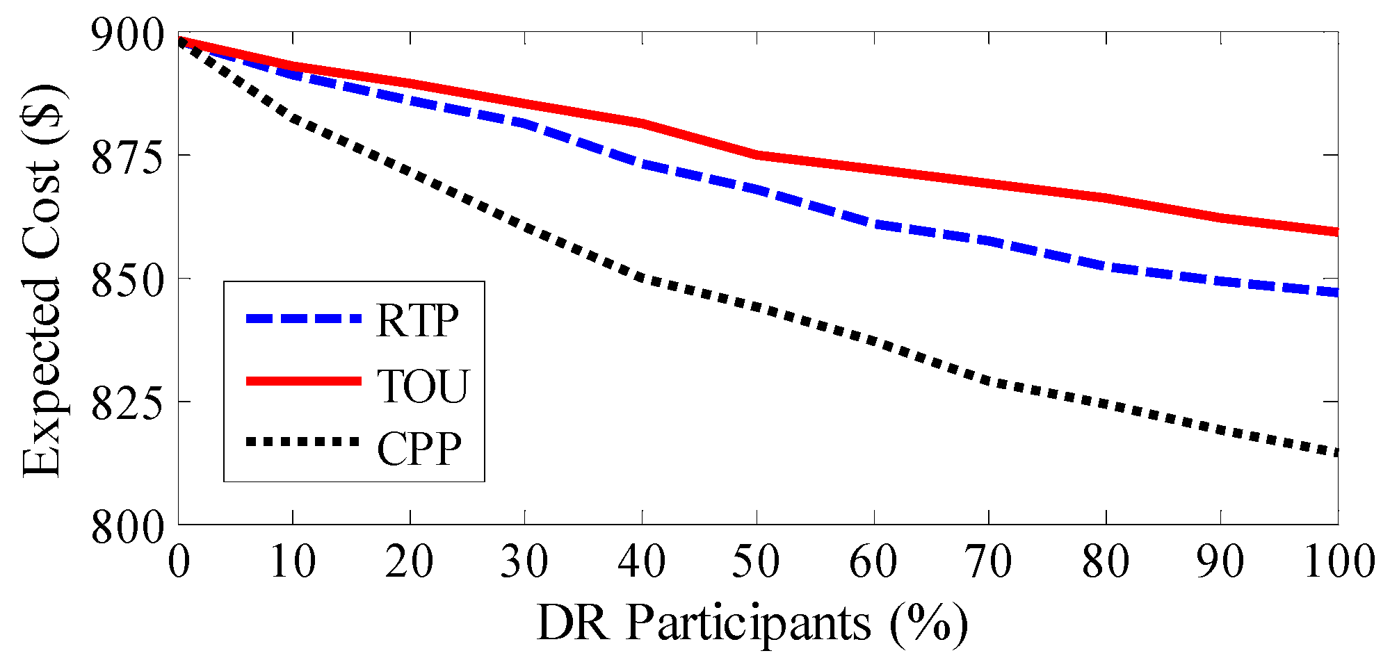
4.2. Presentation and Discussion of Results

We consider the following three cases for testing the effect of scheduling of DR programs and EVs on operation costs of the MG, load profile curve characteristics and profit of customers during the scheduling period.

■

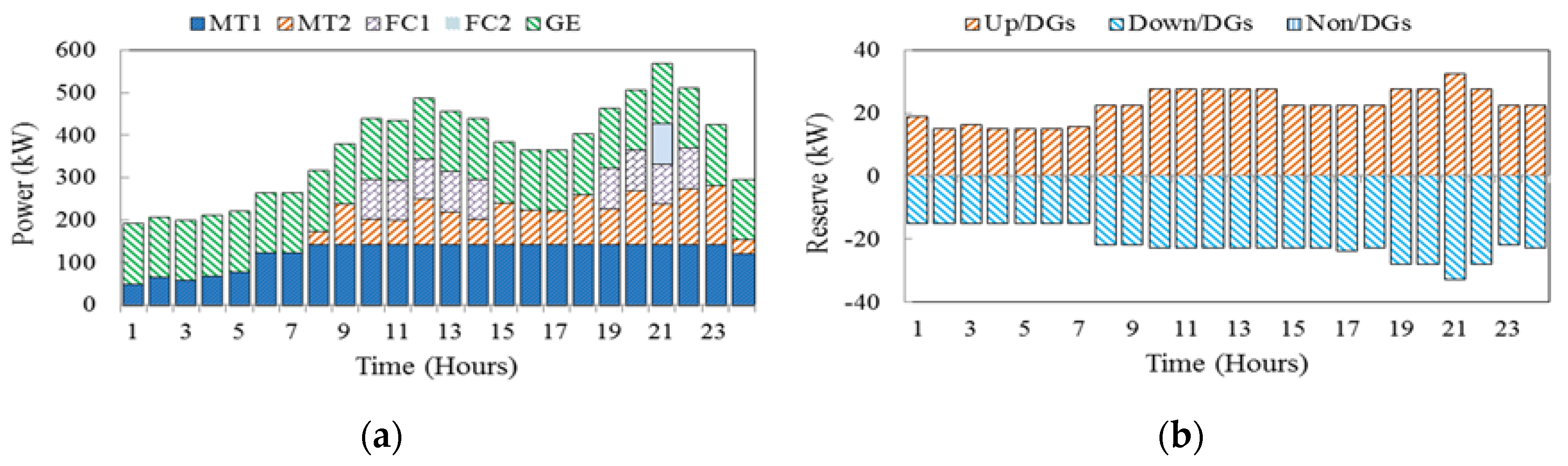
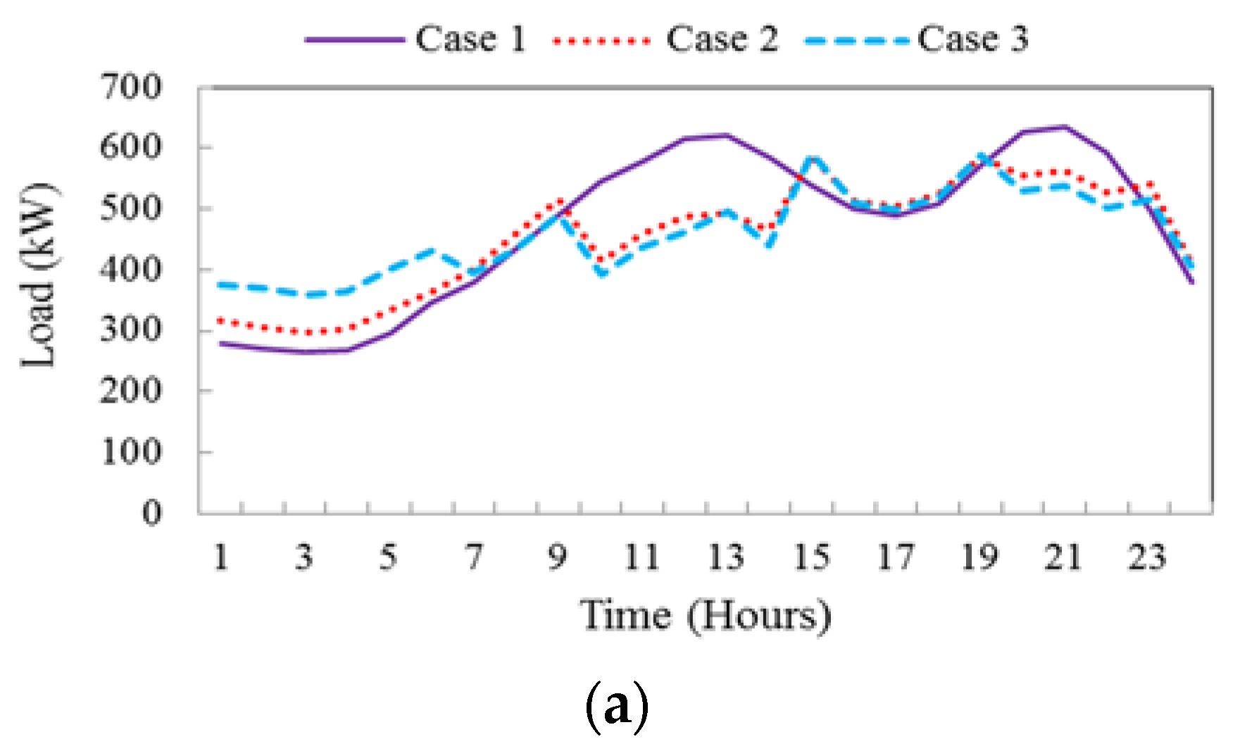
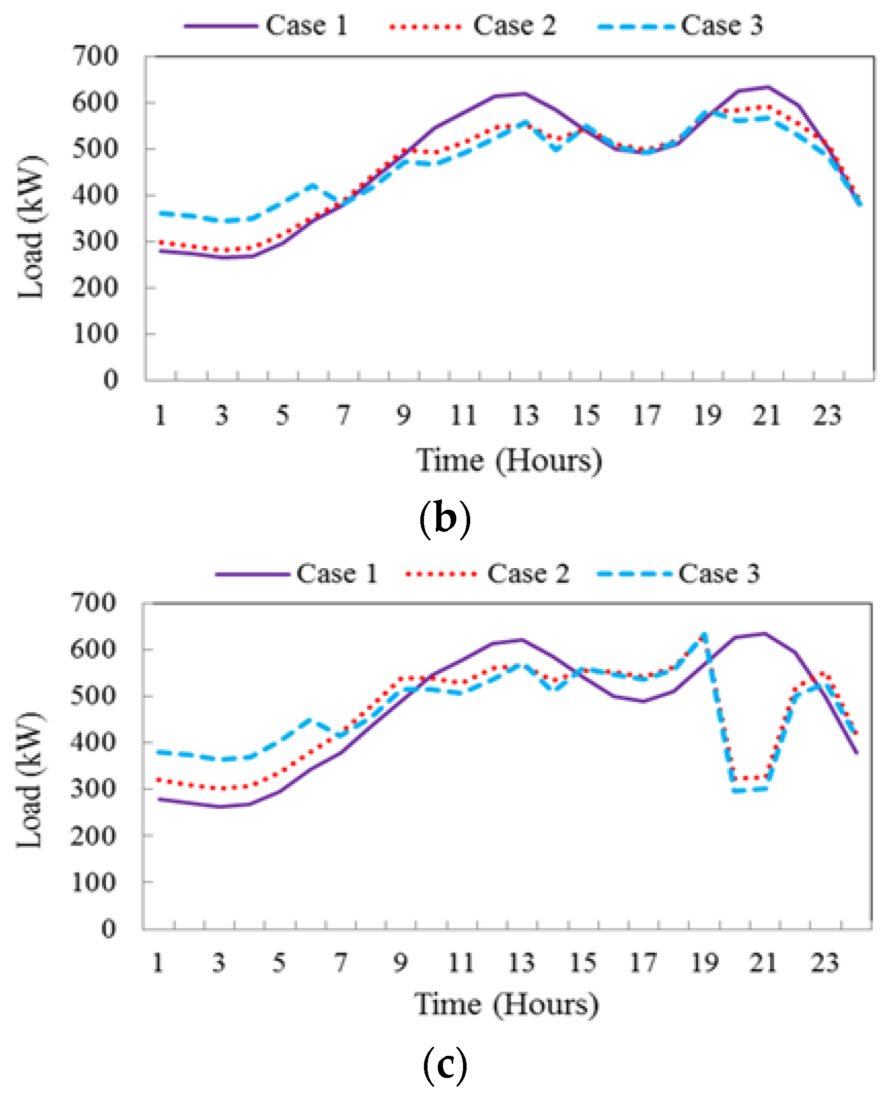
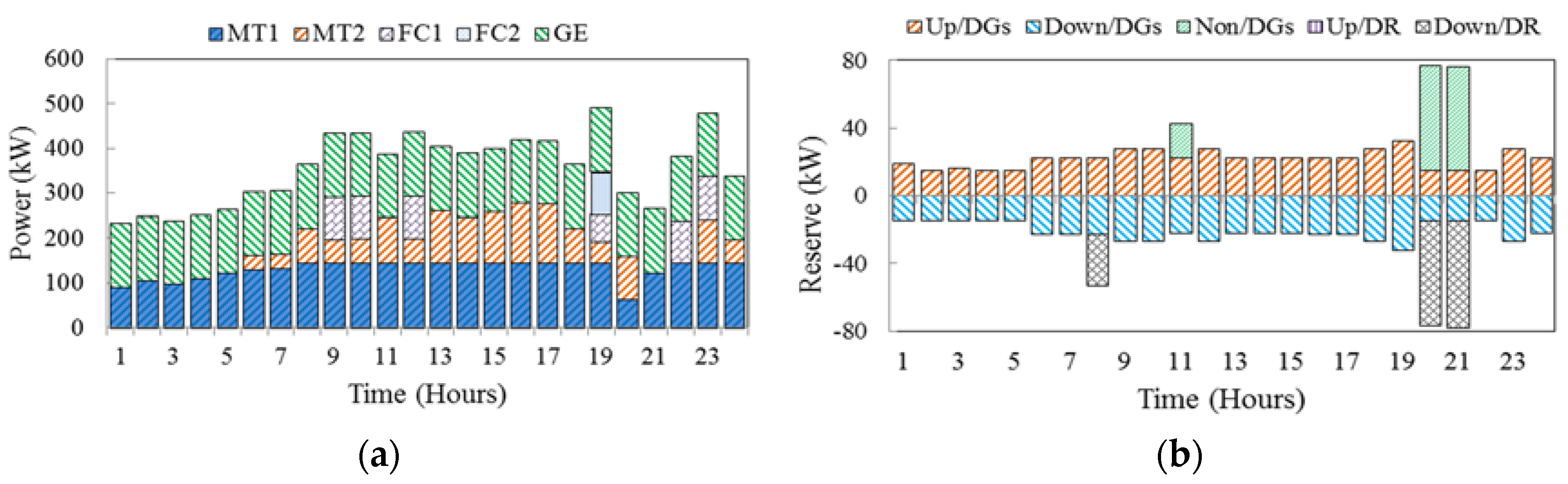
Case 1: without demand side participation and EVs commitment,

■

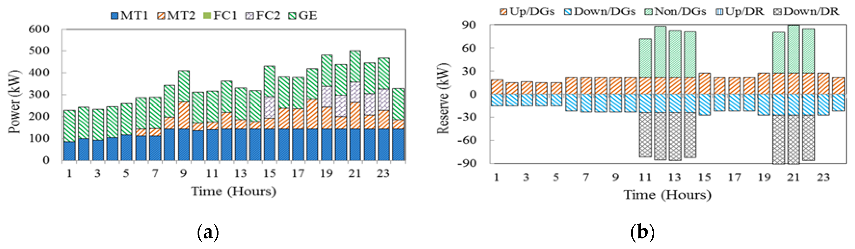
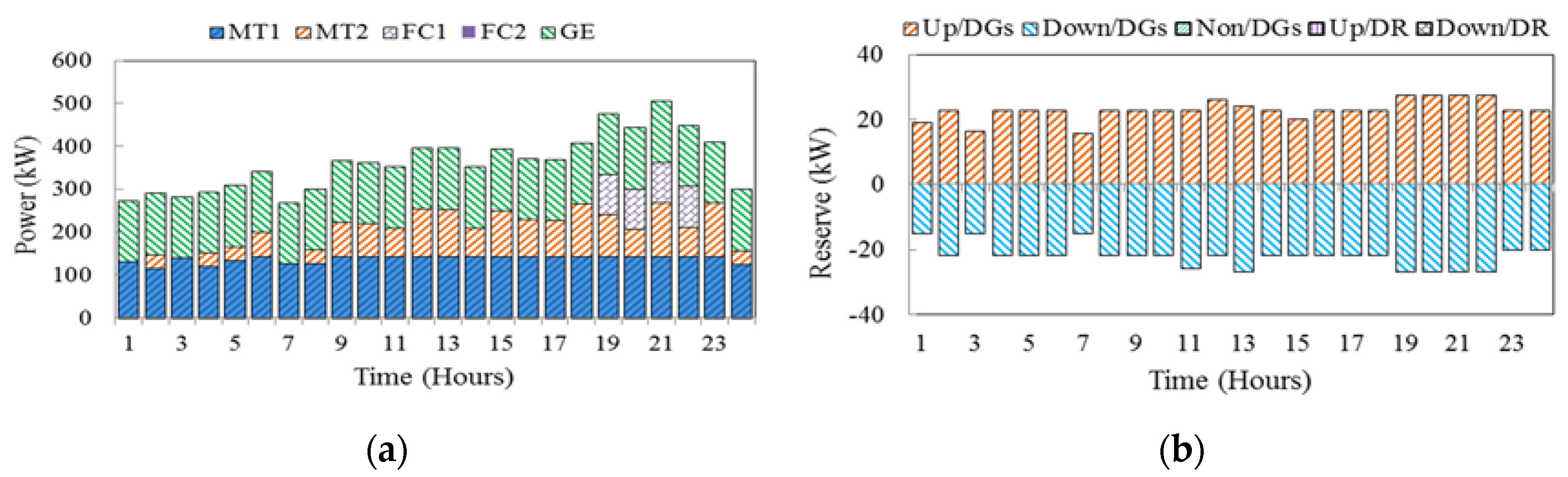
Case 2: with demand side participation and without EVs commitment,

■

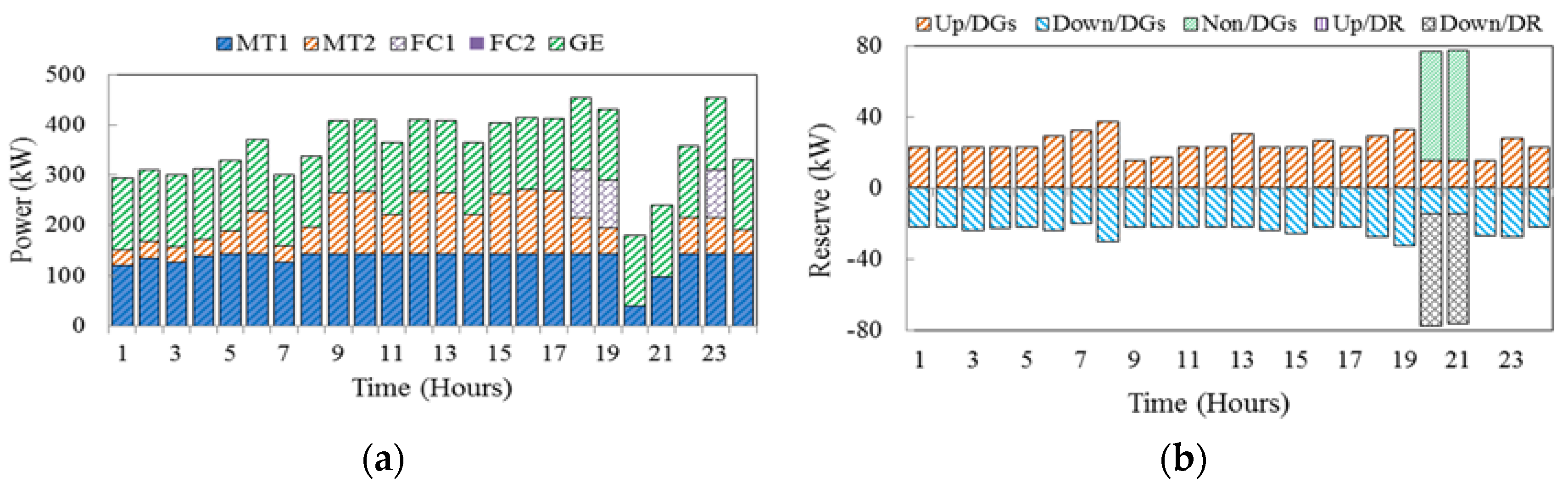
Case 3: with demand side participation and EVs commitment.

It should be noted that Case 1 is considered to be a base case, so operating costs, load profiles and reserve scheduling in other cases are evaluated compared to the base case.

Case 1: In this case, DR programs are not considered and there is no contribution from EVs side. The scheduled energy and reserve capacity in this case is illustrated in Figure 5a,b, respectively. As shown in Figure 5a, based on the economic dispatch results, low-cost MT₁ and GE are used as base units to provide the energy. These generators are dispatched during the entire scheduling horizon to reduce the overall operating cost, while the other units (especially FC₁ and FC₂ due to their higher operating cost) are only dispatched at peak hour periods. As shown in Figure 5b, all the scheduled reserve capacity is provided by dispatchable DG units, including up-spinning reserve (Up/DGs), down-spinning reserve (Down/DGs), and non-spinning reserve (Non/DGs) in this case. Since the output power of WT and PV are intermittent, the required reserve power is provided by MTs, FCs and GE. It can be observed that when RESs power productions in scenarios are relatively different from the forecasted values, (i.e., in 10:00–14:00 and 19:00–22:00), more reserve capacity is scheduled accordingly. The total expected cost of MG operation as well as costs of providing energy and reserve services from DG units in case 1 are obtained as 897.833$, 436.622$ and 19.752$, respectively.

Case 2: In this case, optimal operation of MG with demand-side participation (i.e., TBR-DR programs) but without EVs contribution is presented. The scheduled energy and reserve capacity in RTP programs are illustrated in Figure 6a,b, respectively. Comparing the results in Figure 5a and Figure 6a demonstrates that with demand side participation in RTP schemes, the power provided by DG units is reduced at peak hours, specifically in 10:00–14:00 and 20:00–22:00. Likewise, during the hours with relatively high energy prices, the customers also reduce their consumption levels to save energy and get incentives. On the other hand, customers shift most of their consumptions into the time intervals with low energy prices, specifically in 01:00–05:00 (valley period, see Figure 3) to further reduce their running cost.

As shown in Figure 6b, in this case, a part of the required reserve capacity is provided by demand side participation, including up-spinning reserve (Up/DR) and down-spinning reserve (Down/DR). Comparison of results in Figure 5b and Figure 6b also shows that the participation of responsive loads can decrease the spinning reserve requirement of DG units and reduce the back-up energy costs. It can also be understood from the simulation results that the stochastic nature of wind and PV power generations, makes it necessary to allocate more reserve capacity to the time intervals (e.g., 10:00–14:00 and 19:00–22:00) when the risk of power shortage from RESs is higher. To this end, DR actions can provide a considerable portion of the needed upward reserve in the MG and decrease the MG operation cost. The expected operating cost of MG and the DGs energy and reserve costs in case 2 in RTP program are obtained as 872.943$, 416.789$ and 25.077$, respectively.

The scheduled energy and reserve capacity under TOU programs are illustrated in Figure 7a,b, respectively. By comparing the results in Figure 6a and Figure 7a, it can be seen that the produced powers of DGs in TOU are slightly higher than ones in RTP programs at peak hours. This is due to the fact that during peak periods, participation of consumers in TOU programs is lower than that in RTP programs.

It is also observed from Figure 7b that the scheduled reserves in these programs are different, especially in peak periods. This difference is due to the fact that the load reduction in TOU is less than that of in RTP at peak periods and the customers don’t participate in downward reserve. Therefore, DGs non-spinning reserve scheduling is not required. The expected operating cost of MG and the DGs energy and reserve costs in case 2 under TOU programs are 881.164$, 420.549$ and 19.172$, respectively.

The hourly energy and reserve scheduling in case 2 in CPP programs are shown in Figure 8a,b, respectively. As mentioned before, the electricity price in CPP programs is the same as the price in TOU programs, except during hours 20:00 and 21:00. During these two hours, the price in CPP is four times greater than that of TOU. So, as Figure 8a shows, customers are highly encouraged to reduce their consumption as much as possible. As a result, the demand downward reserve increases in these two hours and consequently, the DGs non-spinning reserve increases. The expected operating cost of MG and the DGs energy and reserve costs are 850.395$, 410.590$ and 21.600$, respectively.

Case 3: In this case, we evaluate the effectiveness of TBR-DR schemes in presence of EVs. In order to indicate the impact of different programs on responsive loads along with the presence of EVs, the same types of tariffs including RTP, TOU and CPP are implemented. Figure 9 illustrates the EVs daily charging and discharging power in different TBR- DR programs. As can be seen from the operating profiles, EVs are charged during low tariff hours (valley periods) and discharged during high tariff hours (peak periods). The energy and reserves scheduling in case 3 are shown in Figure 10a,b.

Compared to Figure 6, it is observed that, the output power of generating units is flattened in the presence of EVs. It should be noted that, in case 3 the charging/discharging powers of EVs are added to the MG load which in turn affect the energy scheduling process; however, there is no effect on the reserve market as EVs are not considered on this occasion. So, it can be seen from Figure 10b that DR provides a part of the required reserve scheduling similar to case 2. The expected operating cost of MG and DGs energy and reserve costs in case 3 in RTP are obtained as 866.113$, 403.482$ and 23.482$, respectively, which are considerably lower than the corresponding values obtained in the previous cases. Thus, an efficient scheduling of EVs and responsive loads can improve the operation of the MG.

Figure 11a,b shows the energy and reserves scheduling in case 3 considering a TOU-based DR program. As can be seen from the results, during peak periods, EVs are discharged, and the operations of the costly units are delayed accordingly. So, in comparison with the two previous cases, the energy cost of DG units decreases. The expected operating cost of MG and DGs energy and reserve costs in case 3 considering a TOU scheme are obtained as 878.252$, 413.482$ and 21.084$, respectively.

The energy and reserves scheduling in case 3 regarding the CPP program are also shown in Figure 12a,b. Also, in this program, the participation of EVs in DR schemes decreases operating costs. The expected operating cost of MG and DGs energy and reserve cost values in this case study are obtained as 853.049$, 400.620$, and 20.801$, respectively.

The total load profile associated with the three cases in TBR programs are illustrated in Figure 13. As can be observed, with the application of DR programs, the total load decreases in peak periods when prices are high and increases in off-peak or valley periods when prices are relatively lower. This leads to smoother load profiles especially in cases 2 and 3. This load-shaping process can be better observed with active participation of EVs and their charging behavior during the valley period (when the price has its lowest value).

It can be also observed from Figure 13a,b, that the load profile in RTP and TOU schemes are relatively similar, but greatly different from the one in CPP scheme (Figure 13c) due to the price spikes at some time intervals and their effect on demand side participation.

Table 3. MG operating costs (in $) in three cases considering TBR-based DR programs.

Attribute	Case 1	Case 2			Case 3
	No DR	RTP	TOU	CPP	RTP	TOU	CPP
Expected cost	897.833	872.943	881.164	850.395	866.113	878.253	853.049
Energy cost of DGs	436.622	416.790	420.549	410.590	403.482	413.482	400.620
Scheduling reserve cost of DGs	19.752	25.076	19.172	21.600	23.482	21.085	22.801
Scheduling reserve cost of DR	0	23.856	0	10.048	33.856	0	10.048
Energy cost of RESs	443.206	443.206	443.206	443.206	443.206	443.206	443.206
Deployed reserve cost of DGs	−2.365	10.182	−2.131	1.536	9.923	−2.081	1.189
Deployed reserve cost of DR	0	−56.785	0	−40.192	−56.785	0	−40.192
Start-up cost of DGs	0.78	0.78	0.62	0.87	0.87	0.64	1.02
Shut-down cost of DGs	0.27	0.27	0.18	0.35	0.35	0.25	0.46

compares the operational costs of the MG in different working conditions. The expected operating cost of MG, DGs and DR scheduled energy and reserve costs, start-up costs and start-down costs have been reported for the three cases. Comparison of results in cases 1 and 2 shows that the deployment of DR programs allows lower total operating cost to be obtained. The reason is that the expensive units are not dispatched to meet the demand of peak periods since peak loads are decreased due to the participation of responsive loads in different DR programs. Also, participation of both responsive loads and EVs in DR programs (case 3) can reduce the total operating cost more than the other cases where there are no DR action or EV support. In fact, in case 3, EVs discharging in peak hours (as shown in Figure 9) causes the decrement of expected cost of MG in comparison with cases 1 and 2. In other words, during peak hours, EVs discharge and supply peak loads; thus, the more expensive units may not be dispatched and, consequently, the energy cost of DGs is reduced. Moreover, in CPP programs, since customers are highly encouraged to reduce their consumption as much as possible at peak hours (at 19:00 and 20:00 as shown in Figure 13), the energy cost of DG units and as the result the total operating cost of MG has its lowest value. Moreover, in case 3, due to the uncertainty of EVs, the total cost of scheduling reserve of DGs and DR in each DR program is more than the one in case 2. However, it can be observed that the total deployed reserve cost of DGs and DR in cases 2 and 3 are almost the same, because deployed reserve is provided by DR and DG units and EVs do not participate, as they only affect the energy scheduling process.

In order to analyze the expected cost of MG with respect to load participation in DR, a sensitivity analysis is done and shown in Figure 14. With increasing customer participation in DR, the expected cost of MG is mitigated in all TBR-DR programs. As observed, in higher values of DR participation (i.e., more than 60%) the expected cost reduced slightly because in higher DR participants, new peaks of demand may occur (also known as rebound peak effect) and expensive units may need to be committed. Also, it is seen that in all the rates of DR participants, the expected cost in CPP program has lower value compared with other TBR-DR programs.

5. Conclusions and Future Work

In this paper, the effect of the TBR-DR programs on reserve and energy scheduling in an isolated residential MG and in the presence of EVs were studied. A two-stage optimization model was developed to minimize the MG operation costs considering RESs and EVs uncertainties. The numerical results revealed that demand-side participation in energy and reserve scheduling reduces the total operating cost in different DR programs. The simulation results also demonstrated that in all TBR-DR programs, the participation of both responsive loads and EVs can reduce the energy cost of DGs and as the result the total operating cost of MG can decrease compared to the case where only DR actions are considered. Comparing the simulation results of TBR-DR programs also demonstrated that in CPP due to a great load reduction at peak price hours, the expected running cost of the system has its lowest value, and as a result, this program could be a proper alternative from the MG operator’s viewpoint. In addition, the results showed that due to the uncertainty of EVs, the total cost of scheduling reserve of DGs and DR in each DR program is more than the one in case only with responsive loads. Moreover, it was shown that by increasing the participation of responsive loads in all TBR-DR programs (i.e., to more than 60%), the rate of decrement of expected cost may reduce due to the rebound peak problem.

Our future efforts will be mainly focused on developing an optimal scheduling model based on real-world uncertainties of DR resources and assessing their effects on islanded MG voltage and frequency security.

References

1. Khodaei, A.; Shahidehpour, M.; Bahramirad, S. A Survey on Demand Response Programs in Smart Grids: Pricing Methods and Optimization Algorithms. IEEE Commun. Surv. Tutor. 2015, 17, 564–571. [Google Scholar]
2. Anvari-Moghaddam, A.; Mokhtari, G.; Guerrero, J.M. Coordinated Demand Response and Distributed Generation Management in Residential Smart Microgrids. In Energy Management of Distributed Generation Systems; Lucian, M., Ed.; InTechOpen: Rijeka, Croatia, 2016; ISBN 978-953-51-4708-4. [Google Scholar]
3. Shariatzadeh, F.; Mandal, P.; Srivastava, A.K. Demand response for sustainable energy systems: A review, application and implementation strategy. Renew. Sustain. Energy Rev. 2015, 45, 343–350. [Google Scholar] [CrossRef]
4. Mohagheghi, S.; Yang, F.; Falahati, B. Impact of demand response on distribution system reliability. In Proceedings of the IEEE PES General Meeting, San Diego, CA, USA, 24–28 July 2011. [Google Scholar]
5. Palensky, P.; Dietmar, D. Demand side management: Demand response, intelligent energy systems smart loads. IEEE Trans. Ind. Inform. 2011, 7, 381–388. [Google Scholar] [CrossRef]
6. Nguyen, D.T.; Negnevitsky, M.; de Groot, M. Pool-based demand response exchange-concept and modeling. IEEE Trans. Power Syst. 2011, 26, 1677–1685. [Google Scholar] [CrossRef]
7. Aghajani, G.R.; Shayanfar, H.A.; Shayeghi, H. Presenting a multi-objective generation scheduling model for pricing demand response rate in micro-grid energy management. Energy Convers. Manag. 2015, 106, 308–321. [Google Scholar] [CrossRef]
8. Jovanovic, R.; Bousselham, A.; Safak Bayram, I. Residential Demand Response Scheduling with Consideration of Consumer Preferences. Appl. Sci. 2016, 6, 16. [Google Scholar] [CrossRef]
9. Anvari-Moghaddam, A.; Rahimi-Kian, A.; Monsef, H. Optimal Smart Home Energy Management Considering Energy Saving and a Comfortable Lifestyle. IEEE Trans. Smart Grid 2015, 6, 324–332. [Google Scholar] [CrossRef]
10. Babar Rasheed, M.; Javaid, N.; Ahmad, A.; Ali Khan, Z.; Qasim, U.; Alrajeh, N. An Efficient Power Scheduling Scheme for Residential Load Management in Smart Homes. Appl. Sci. 2015, 5, 1134–1163. [Google Scholar] [CrossRef]
11. Rodriguez-Diaz, E.; Anvari-Moghaddam, A.; Vasquez, J.C.; Guerrero, J.M. Multi-Level Energy Management and Optimal Control of a Residential DC Microgrid. In Proceedings of the 35th IEEE International Conference Consumer Electronics (ICCE), Las Vegas, NV, USA, 8–11 January 2017. [Google Scholar]
12. Rabiee, A.; Sadeghi, M.; Aghaeic, J.; Heidari, A. Optimal operation of microgrids through simultaneous scheduling of electrical vehicles and responsive loads considering wind and PV units uncertainties. Renew. Sustain. Energy Rev. 2016, 57, 721–739. [Google Scholar] [CrossRef]
13. Alvarez, E.; Campos, A.M.; Arboleya, P.; Gutiérrez, A.J. Microgrid management with a quick response optimization algorithm for active power. Int. J. Electr. Power Energy Syst. 2012, 43, 465–473. [Google Scholar] [CrossRef]
14. Anvari-Moghaddam, A.; Seifi, A.R.; Niknam, T.; Alizadeh Pahlavani, M.R. Multi-objective operation management of a renewable MG (microgrid) with back-up micro-turbine/fuel cell/battery hybrid power source. Energy 2011, 36, 6490–6507. [Google Scholar] [CrossRef]
15. Anvari-Moghaddam, A.; Seifi, A.R.; Niknam, T. Multi-operation management of a typical microgrid using Particle Swarm Optimization: A comparative study. Renew. Sustain. Energy Rev. 2012, 16, 1268–1281. [Google Scholar] [CrossRef]
16. Chaouachi, A.; Kamel, R.M.; Andoulsi, R.; Nagasaka, K. Multiobjective intelligent energy management for a microgrid. IEEE Trans. Ind. Electron. 2013, 60, 1688–1699. [Google Scholar] [CrossRef]
17. Karangelos, E.; Bouffard, F. Towards full integration of demand-side resources in joint forward energy/reserve electricity markets. IEEE Trans. Power Syst. 2010, 27, 280–289. [Google Scholar] [CrossRef]
18. Shan, J.; Botterud, A.; Ryan, S.M. Impact of demand response on thermal generation investment with high wind penetration. IEEE Trans. Smart Grid 2013, 4, 2374–2383. [Google Scholar]
19. Peng, X.; Jirutitijaroen, P. A stochastic optimization formulation of unit commitment with reliability constraints. IEEE Trans. Smart Grid 2013, 4, 2200–2208. [Google Scholar]
20. Vrakopoulou, M.; Margellos, K.; Lygeros, J.; Andersson, G. A prob-abilistic framework for reserve scheduling and N-1 security assessment of systems with high wind power penetration. IEEE Trans. Power Syst. 2013, 28, 885–3896. [Google Scholar] [CrossRef]
21. Paterakis, N.G.; Erdinc, O.; Bakirtzis, A.G.; Catalão, J.P.S. Load-Following Reserves Procurement Considering Flexible Demand-Side Resources under High Wind Power Penetration. IEEE Trans. Power Syst. 2015, 30, 1337–1350. [Google Scholar] [CrossRef]
22. Aghaei, J.; Ahmadi, A.; Rabiee, A.; Agelidis, V.G.; Muttaqi, K.M.; Shayanfar, H. Uncer-tainty management in multiobjective hydro-thermal self-scheduling under emission considerations. Appl. Soft Comput. 2015, 37, 737–750. [Google Scholar] [CrossRef]
23. Amjady, N.; Aghaei, J.; Shayanfar, H.A. Stochastic multiobjective market clearing of joint energy and reserves auctions ensuring power system security. IEEE Trans. Power Syst. 2009, 24, 1841–1854. [Google Scholar] [CrossRef]
24. Dong, Q.; Yu, L.; Song, W.Z.; Tong, L.; Tang, S. Distributed demand and response algorithm for optimizing social-welfare in smart grid. In Proceedings of the 26th IEEE IPDPS, Shanghai, China, 21–25 May 2012; pp. 1228–1239. [Google Scholar]
25. Gholami, A.; Shekari, T.; Aminifar, F.; Shahidehpour, M. Microgrid Scheduling with Uncertainty: The Quest for Resilience. IEEE Trans. Smart Grid 2016, 30, 1337–1350. [Google Scholar] [CrossRef]
26. Kirschen, D.S.; Strbac, G. Fundamentals of Power System Economics; Wiley: Hoboken, NJ, USA, 2004. [Google Scholar]
27. Abdollahi, A.; Parsa-Moghaddam, M.; Rashidinejad, M.; Sheikh-El-Eslami, M.K. Investigation of Economic and Environmental-Driven Demand Response Measures Incorporating UC. IEEE Trans. Smart Grid 2012, 3, 12–25. [Google Scholar] [CrossRef]
28. Ma, Y.; Houghton, T.; Cruden, A.; Infield, D. Modeling the Benefits of Vehicle-to-Grid Technology to a Power System. IEEE Trans. Power Syst. 2012, 27, 1012–1020. [Google Scholar] [CrossRef]
29. Zakariazadeh, A.; Jadid, S.; Siano, P. Smart microgrid energy and reserve scheduling with demand response using stochastic optimization. Electr. Power Energy Syst. 2014, 63, 523–533. [Google Scholar] [CrossRef]
30. Rezaei, N.; Kalantar, M. Smart microgrid hierarchical frequency control ancillary service provision based on virtual inertia concept: An integrated demand response and droop controlled distributed generation framework. Energy Convers. Manag. 2015, 92, 287–301. [Google Scholar] [CrossRef]
31. Youcef, F.; Mefti, A.; Adane, A.; Bouroubi, M. Statistical analysis of solar measurements in Algeria using beta distributions. Renew. Energy 2002, 26, 47–67. [Google Scholar] [CrossRef]
32. Anvari-Moghaddam, A.; Monsef, H.; Rahimi-Kian, A.; Nance, H. Feasibility Study of a Novel Methodology for Solar Radiation Prediction on an Hourly Time Scale: A Case Study in Plymouth, UK. J. Renew. Sustain. Energy 2014, 6, 033107. [Google Scholar] [CrossRef]
33. Arthur, D.; Vassilvitskii, S. k-means++: The advantages of careful seeding. In Proceedings of the 18th Annual ACM-SIAM Symposium Discrete Algorithms (SODA ‘07), New Orleans, LA, USA, 7–9 January 2007; pp. 1027–1035. [Google Scholar]
34. Rezaei, N.; Kalantar, M. Stochastic frequency-security constrained energy and reserve management of an inverter interfaced islanded microgrid considering demand response programs. Int. J. Electr. Power Energy Syst. 2015, 69, 273–286. [Google Scholar] [CrossRef]
35. Rassaei, F.; Soh, W.S.; Chua, K.C. Demand Response for Residential Electric Vehicles with Random Usage Patterns in Smart Grids. IEEE Trans. Sustain. Energy 2015, 6, 1367–1376. [Google Scholar] [CrossRef]
36. Vahedipour-Dahraei, M.; Rashidizadeh-Kermani, H.; Najafi, H.R. A Proposed Strategy to Manage Charge/Discharge of EVs in a Microgrid Including Renewable Resources. In Proceedings of the 24th Iranian Conference on Electrical Engineering (ICEE), Shiraz, Iran, 10–12 May 2016; pp. 649–654. [Google Scholar]
37. The General Algebraic Modeling System (GAMS) Software. Available online: http://www.gams.com (accessed on 15 September 2016).
Figure 1. Single line diagram of the simulated microgrid MG.
Applsci 07 00378 g001
Figure 2. The output power of renewable energy resources (RESs) in the reduced generated scenarios, (a) each wind turbine (WT) and (b) each photovoltaic (PV) plant.
Applsci 07 00378 g002
Figure 3. Total demand load curve of MG.
Applsci 07 00378 g003
Figure 4. Energy prices at different tariffs (RTP, TOU and CPP).
Applsci 07 00378 g004
Figure 5. Hourly energy and reserves scheduling in case 1, (a) hourly energy and (b) reserve capacity.
Applsci 07 00378 g005
Figure 6. Hourly energy and reserves scheduling in case 2 under RTP programs (a) energy and (b) reserve.
Applsci 07 00378 g006
Figure 7. Hourly energy and reserves scheduling in case 2 under TOU programs (a) energy and (b) reserve.
Applsci 07 00378 g007
Figure 8. Hourly energy and reserves scheduling in case 2 under CPP programs (a) energy and (b) reserve.
Applsci 07 00378 g008
Figure 9. Charging and discharging power of EVs in TBR-based DR programs.
Applsci 07 00378 g009
Figure 10. Hourly energy and reserves scheduling in case 3 in RTP programs (a) hourly energy and (b) Reserve.
Applsci 07 00378 g010
Figure 11. Hourly energy and reserves scheduling in case 3 in TOU programs (a) hourly energy and (b) Reserve.
Applsci 07 00378 g011
Figure 12. Hourly energy and reserves scheduling in case 3 in CPP programs (a) hourly energy and (b) Reserve.
Applsci 07 00378 g012
Figure 13. Daily load profile in three cases considering (a) RTP, (b) TOU and (c) CPP programs.
Applsci 07 00378 g013aApplsci 07 00378 g013b
Figure 14. Expected cost of MG versus customers’ participation in different TBR-DR programs.
Applsci 07 00378 g014