Helicopter Blade-Vortex Interaction Airload and Noise Prediction Using Coupling CFD/VWM Method

National Laboratory of Science and Technology on Rotorcraft Aerodynamics, Nanjing University of Aeronautics and Astronautics, Nanjing 210000, China
*
Author to whom correspondence should be addressed.
Appl. Sci. 2017, 7(4), 381; https://doi.org/10.3390/app7040381
Submission received: 13 January 2017
/
Revised: 7 April 2017
/
Accepted: 7 April 2017
/
Published: 11 April 2017
Abstract
:As a high resolution airload with accurate rotor wake is pivotal for rotor BVI (Blade-vortex interaction) analysis, a hybrid method with combined Navier-Stokes equation, viscous wake model, and FW-H (Ffowcs Williams-Hawkings) equation is developed for BVI airload and noise in this paper. A comparison with the CFD (Computational Fluid Dynamics)/FW-H method for the AH-1/OLS (Operational Load Survey) rotor demonstrates its capability for favorable accuracy and high computation efficiency. This paper further discusses the mechanisms for the impacts of four flight parameters (i.e., tip-path-plane angle, thrust coefficient, tip Mach number, advance ratio) on BVI noise. Under the BVI condition, several BVI events concurrently occur on the rotor disk. Each interaction has a distinct radiation direction which depends on the interaction azimuth, and its noise intensity is highly associated with the characteristic parameters (e.g., miss-distance, interaction angle, vortex strength). The BVI noise is dominated by the interactions at 30–90° in azimuth on the advancing side, of which the wake angle range is from 180° to 540°. Furthermore, the tip-path-plane angle, thrust coefficient, and tip Mach number change the noise intensity mainly via miss-distance, interaction angle, and vortex strength, but for different advance ratios, the noise intensity and propagation direction are more dependent on the interaction angle and interaction azimuth.
1. Introduction
It is well known that helicopter rotor impulsive noise originates from high-speed impulsive noise, which is due to a high tip Mach number on the rotor’s advancing side, and the blade-vortex interaction noise on the advancing and retreating sides of the rotor disk. Blade-vortex interaction (BVI) [1] occurs when the strong tip vortices shed from the main rotor pass in close to the following blades during descending or maneuvering flight; this results in impulsive changes in blade loading, which radiates noise. Not only does BVI noise have significant effects on passenger comfort but the vibratory loads also increase pilot workload and maintenance costs. The calculation and analysis of BVI noise remain a challenging task in the field of helicopter aerodynamics and aerodynamic acoustics [2].
The BVI aerodynamic load and noise strength, as well as the radiation direction, relate to many factors, such as the location of BVI events, the blade tip vortex structure, and the miss-distance. Within the past several decades, considerable effort has been devoted towards noise mechanisms and the alleviation of BVI [3,4,5,6], but most of these studies have been focused on experiments. In numerical studies, the complexity of BVI renders simulation and analysis more difficult, consequently slowing its development. The rotor wake structure and the unsteady aerodynamic load distribution on the blade surface have been recognized as the most important parameters in order to better predict BVI noise. In 1990s, the computational fluid dynamics (CFD) method was gradually applied to rotor aerodynamic research [7,8,9,10]. Some scholars further utilized this method to study BVI aerodynamics and noise [11,12,13]. However, the numerical dissipation inherent in the difference schemes and the interpolation errors make it hard to accurately capture the rotor tip vortices. Despite grid refinement, high order-accuracy schemes and adaptive grids can be used to reduce numerical dissipation, but these methods are still insufficient at capturing the wake structure entirely; furthermore, vast amounts of computation time and resources limit their applications in researching the rotor BVI problem. In recent years, a coupled method combining the wake model with the Euler solver was developed [14,15,16,17] and several remarkable studies on BVI noise have been reported in [18,19] demonstrating the capability of the coupled method to predict BVI noise; however, the wake solutions rely on empirical formulations due to the assumption of inviscid flow, resulting in some errors regarding BVI airload prediction.
To overcome the deficiencies of the existing coupled methods in BVI noise prediction, a high-resolution method coupling CFD and the viscous wake method (VWM), developed by Shi et al. in [20,21], is employed for rotor wake simulation and impulsive airload calculation, and the generalized Farassat formulation based on the Ffowcs Williams-Hawkings (FW-H) Equation [22] is applied for noise prediction. The details of the coupled method are described in this paper. To validate this method, the rotor wake structure, blade airload, and noise characteristics are performed for the AH-1/OLS (Operational Load Survey) rotor under the BVI condition, and we present a comparison between it and the CFD/FW-H method. In addition, important parameters for governing BVI noise have been identified: the tip-path-plane angle, the thrust coefficient, the tip Mach numbers and the advance ratio. This work further examines the mechanisms for the effects of these four parameters on BVI noise amplitude and propagation direction by analyzing the effects of those on the characteristic parameters under different flight conditions.
2. Computational Method
2.1. Aerodynamic Model
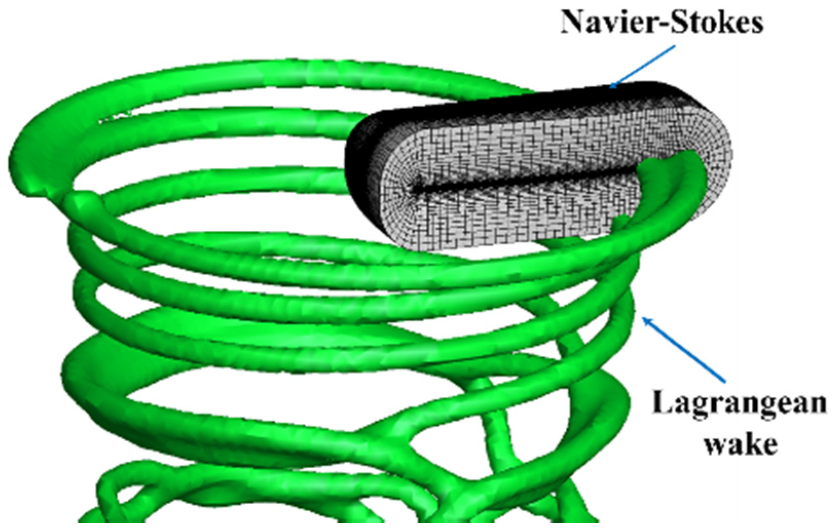
The prerequisite for predicting BVI noise is accurate calculation of the unsteady impulsive airload on the blade surface. As Figure 1 shows, the flow field is divided into two zones in the coupled method: a Navier-Stokes code is used to model the tip vortex generation region, and a viscous wake model is used to account for the effect of the far wake.
2.1.1. Navier-Stokes Solver
In the area around the rotor grid computational domain, the conservation form of the Navier-Stokes equation is established to capture the nonlinear characteristics and wake generation in the near-body zone. With the coordinate system defined on the inertial system, the equation can be expressed as
where is the cell volume, and denotes the face area. and are the convective (inviscid) and the viscous flux vectors, respectively, is the vector of conserved variables and , . and are the density and energy, respectively.
In this paper, a dual-time stepping method is applied for the time discretization to solve the governing equation. LU-SGS (Lower-upper Symmertric Gauss-Seidel) [23] is adopted for sub-iteration at every pseudo-time step. The inviscid terms are calculated by the Roe scheme [24], and the Baldwin-Lomax model is employed as the turbulence model for the Reynolds Averaged Navier-Stokes (RANS) closure.
2.1.2. Viscous Wake Model
As the wake movement is independent of the initial conditions after leaving the rotor at a distance, the Lagrangian-based viscous wake method [25] is adopted. In the VWM, the wake vorticity is discretized into a set of regular distributed vortex particles, and the process of wake rollup, distortion, and dissipation is numerically simulated with a Lagrangian description. The discrete vorticity field can be described by the vorticity kinematic and dynamic equations [21]:
where is the position of the particle, is the vector-valued total vorticity inside the particle , , is the free stream velocity, and is the local induced velocity. In the right-hand side of Equation (3), the first term is the stretching-effect term and the velocity field is analytically differentiated to solve the velocity gradient. The second term is the viscous diffusion term, and the Particle Strength Exchange (PSE) method [26] is utilized for the solution.
For the viscous wake simulation, the blade surface is treated as a vorticity source that sheds the vorticity into the rotor wake. At one time-step, between the n-th blade azimuth and the (n + 1)-th blade azimuth, new vortex particles are generated behind each rotor blade for azimuthal and radial variation of the bound circulation. The radial and time derivatives of the bound vortex denote the circulation of the trailed and shed vortices, respectively. Therefore, the vorticity of new vortex particles is expressed as follows:
where is the blade-bound vortex circulation at the (n + 1)-th azimuth, and is the relative velocity of the blade section at the (n + 1)-th azimuth due to the free stream velocity, rotor rotation velocity, and blade flapping velocity. The total vorticity source is distributed onto an interpolation surface which represents the convected trajectory of the blade during that time-step. An equal annulus area rule is adopted for the blade spanwise discretization for aerodynamics. The vorticity variation of the new vortex particles shed into the rotor wake is governed by Equation (3) and the vorticity strength in it is obtained by the following formulation:
where is the volume of particle p, which takes the product of the cross-sectional area and the length of the filament segment p, as the new vorticity is discreted into a set of filament segments with the vortex core radius during the time-step.
2.1.3. Coupling Algorithm
The “integrated vorticity approach” [21] is utilized to transmit the vorticity from the CFD solution to the VWM. In this approach, the blade spanwise load distribution is first calculated using the Navier-Stokes equation; the bound vortex circulation is calculated by the Kutta-Joukowski theorem:
where is the lift coefficient of the blade section obtained by integrating the pressure on the blade surface. The vorticity of new vortex passed to the viscous wake method (VWM) is calculated by the tip vortex strength using Equations (4) and (5).
The “outer boundary correction” approach [21] is adopted to pass the induced velocity from the VWM which is only imposed on the outer boundary of the blade grid to the CFD domain. At the outer boundary of the CFD domain, the velocity, density, energy, and pressure are obtained from the following equations:
here, are the free-stream velocities, are the blade moving velocities, and are the wake induced velocities. is the ratio of specific heats and is the local Mach number. The subscript denotes the free stream.
2.2. Acoustic Model
Noise prediction in the current work depends on the well-known Ffowcs Williams-Hawkings (FW-H) Equation which is based on the Lighthill acoustic analogy method. Monopole and dipole sources physically denote the blade thickness and loading noise, and the quadrupole source involves the nonlinear effect from the flow-field compression. In this paper, it is assumed that the contribution to noise from the quadrupole term is negligible which simulates nonlinear noise at high speed, as strong blade-vortex interactions are known to occur at low-speed descent conditions. The integral formulation 1A developed by Farassat [22] is used in BVI noise prediction, i.e.,
where
The subscript indicates that the integrals are evaluated at the retarded time . The blade surface is divided into panels and the loads from each panel are used to obtain the total noise by integration. More descriptions about F1A formulation can be found in [22].
Figure 2 shows the flowchart of the BVI airload and noise prediction. The calculation process of this method mainly includes three parts: (1) Calculate the spanwise sectional circulation around the blade using CFD and pass the vorticity to the VWM module; (2) Generate the source term, solve the rotor wake and the induced velocity using VWM, and feed the induced velocity back to the CFD domain; (3) Based on the desired precision, select the blade surface element, calculate the corresponding retarded time on the basis of observation time and location, and predict the BVI noise sound radiation using the FW-H equation.
3. Results and Discussions
To validate the BVI prediction capability of the CFD/VWM/FW-H method, the AH-1/OLS rotor model under the BVI condition is performed in this section. A parametric study on the blade airload and BVI noise is further carried out.
3.1. Numerical Setup
The two-bladed AH-1/OLS rotor model considered has a diameter of R = 1.916 m, an aspect ratio of 9.22 and a BHT-540 symmetric airfoil. The rotor model operates at , , , , which is the baseline of the computational parameters in the following parametric study. Specifically, the control inputs are shown in Table 1 from the experimental data [3]. The longitudinal pitch and lateral flapping (resp. lateral cyclic and longitudinal flapping), refer to the SIN component (resp. COS) of the first harmonic. The numerical condition is presented in Table 2.
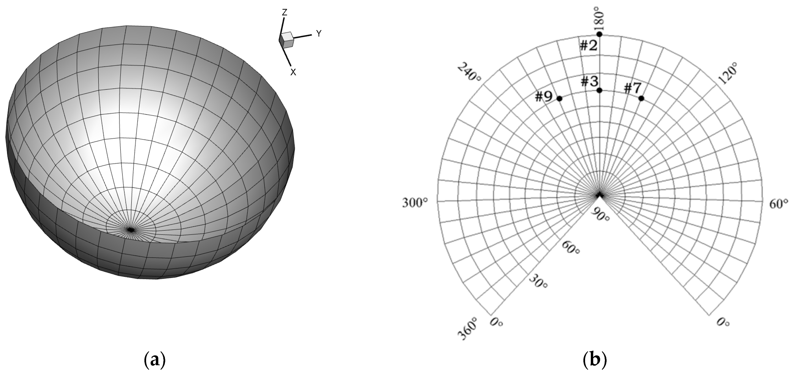
The observation locations in the numerical simulation, same with the microphones in the test condition, are distributed on a spherical surface, 3.44 R from the rotor hub, as seen in Figure 3a. The Lambert projection is applied for turning the acoustic radiation spherical arc into a plane for better observation, and Figure 3b shows the projection developed drawing.
3.2. Analysis of BVI Airload and Noise
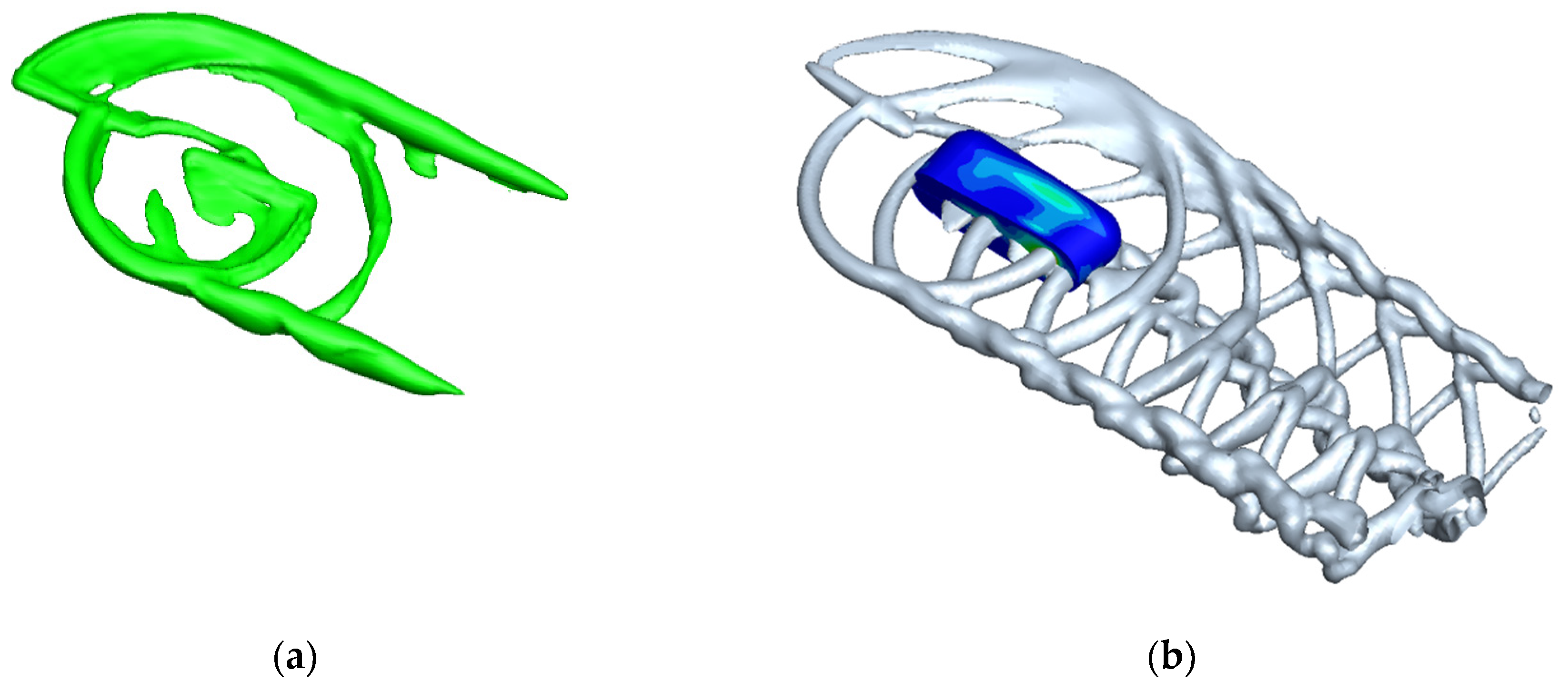
As the rotor wake has been recognized as one of the most important parameters for generating BVI noise, the vorticity iso-surfaces calculated using the full CFD method and the coupling CFD/VWM method are shown in Figure 4, and the non-dimensional vorticity magnitudes of both methods are set as 0.4. With the rotor wake influenced by forward flow and induced velocity, the formation and rollup of the rotor tip vortex occur on both the advancing and retreating sides; two more intense vortex bunches form there. However, the prominent diffusion in the wake-developing zone is observed in the full CFD method, reflecting that the numerical dissipation problem causes the vorticity to diffuse rapidly. By contrast, in the coupling method, the rotor wake is well preserved when traveling downstream. This indicates that the coupling method is capable of capturing distortion and the wake boundary, effectively improving the numerical dissipation problem in the CFD domain, and enhancing the ability to capture the BVI characteristics.
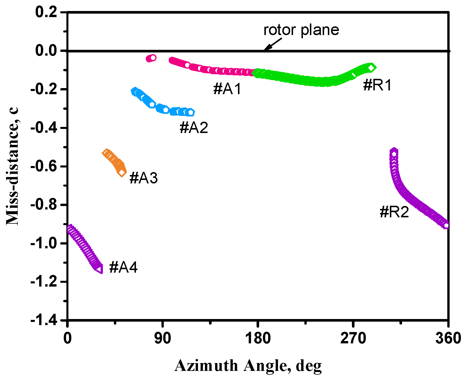
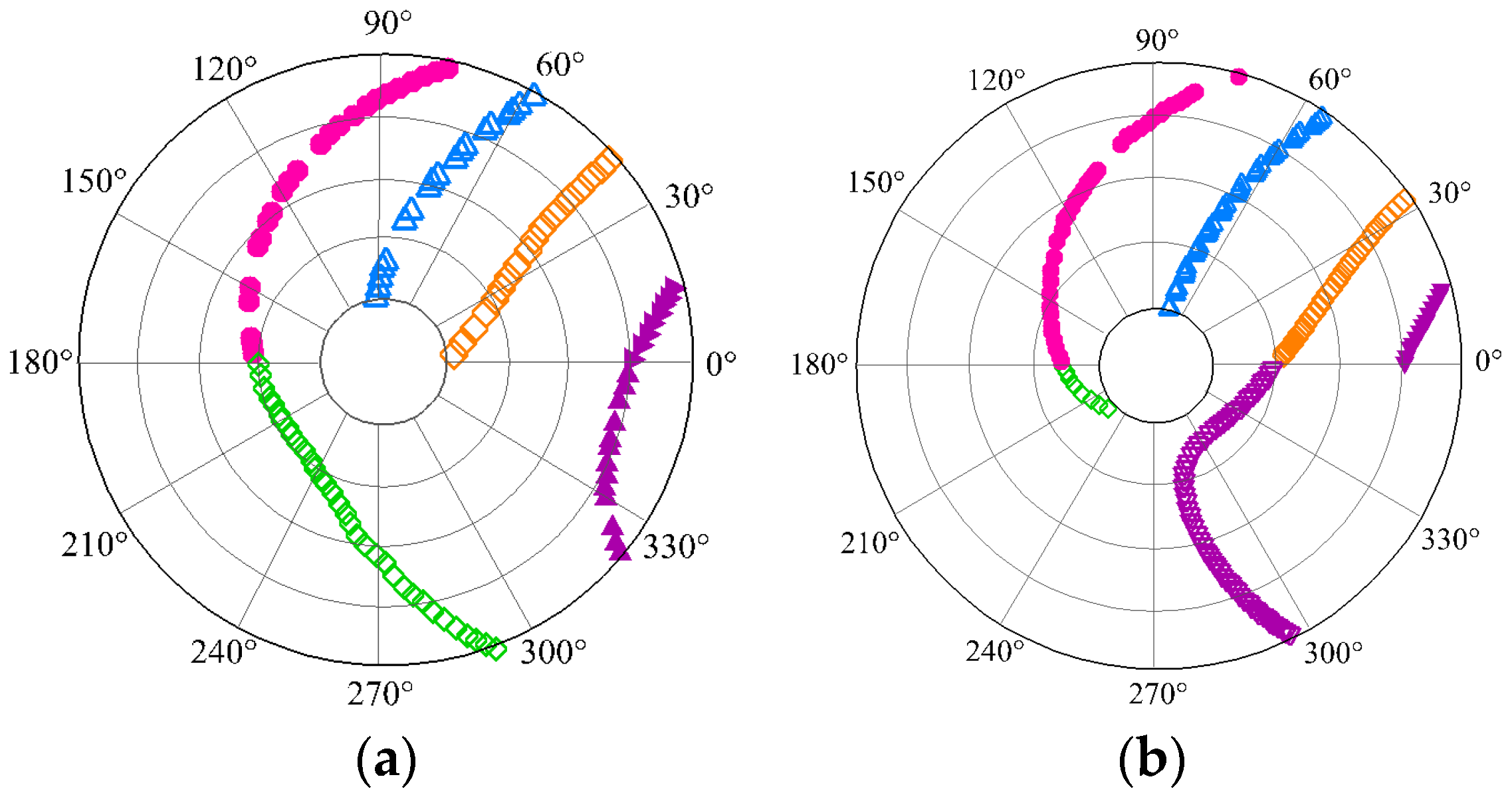
During descent flight, specific BVI events are observed at several azimuth angles. Utilizing the blade and tip vortex geometry equations in Sim et al.’s research [27], we can capture the BVI loci. Figure 5 shows the locations of BVI events and the lift distribution on the rotor disk. Six BVI events are identified in Figure 5a, of which four on the advancing side are marked as: #A1, #A2, #A3, #A4, and the other two on the retreating side are marked as: #R1, #R2. Figure 5b shows that complicated lift fluctuations occur near the locations of BVI events. According to the relative position between the blade and the vortex filament, the interactions #A3 and #R2 in the outer part of the blade are referred to as parallel interactions, because each blade’s leading edge is nearly parallel to the vortex filament, while others are referred to as oblique interactions. Figure 6 presents the miss-distance, which varies with the azimuth angle on the axial plane, and the interaction strength of BVI depends on both the interaction angle and the miss-distance.
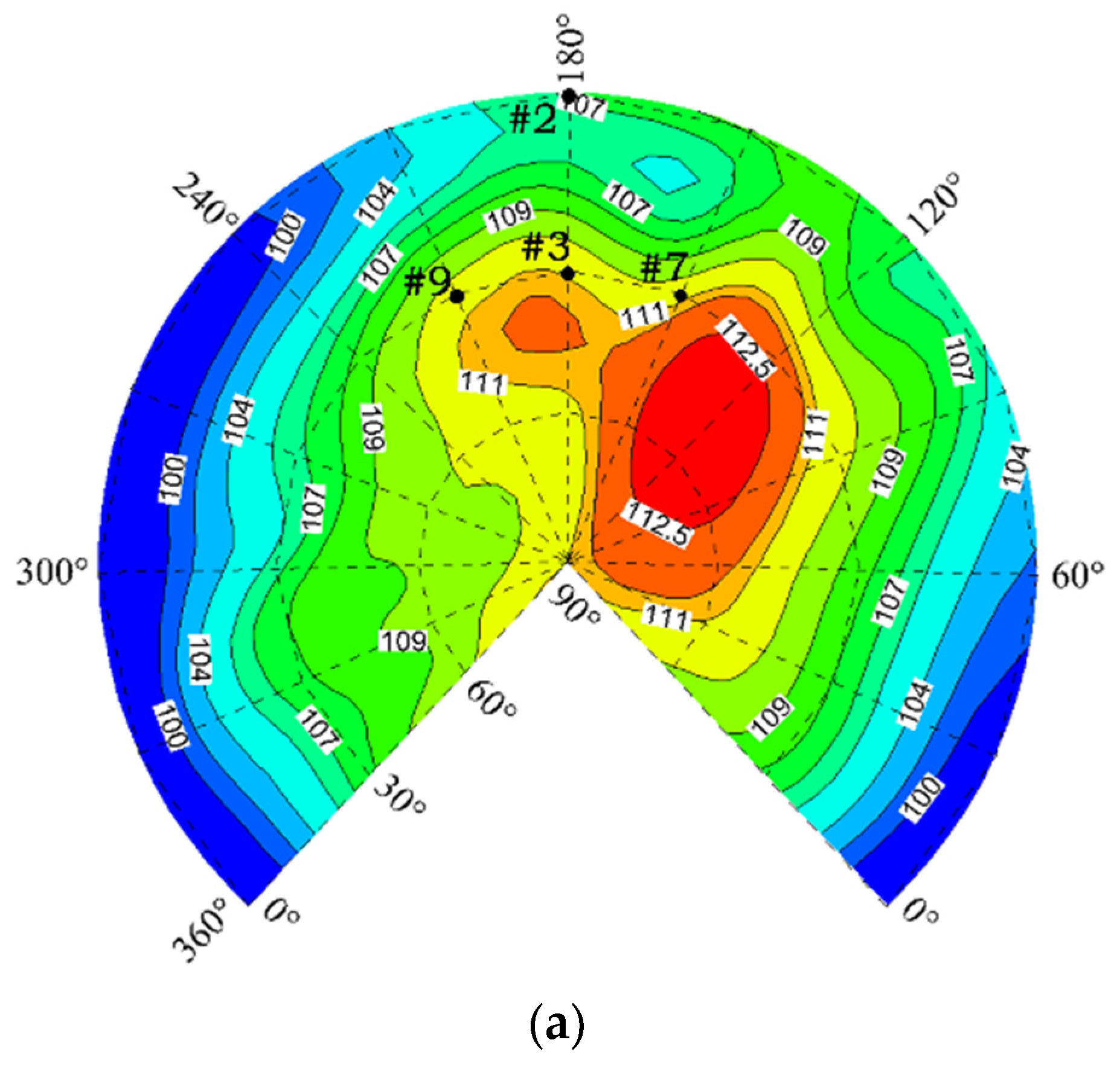
The contour plots of SPL on the 3.44 R hemi-spherical surface are shown in Figure 7a. As shown, the high noise level (acoustic “hotspot”) appears at 120° in azimuth and 45° below the rotor plane, implying that the typical BVI noise has strong directivity, approximately down and forward from the rotor. Figure 7b presents the predicted sound pressure distributions using the CFD/VWM/FW-H method at four observation locations (#2, #3, #7, #9). For comparison, the results of using the CFD/FW-H method are also included in the figures. BVI noise is found to dominate at #3, #7, and #9, and each noise signature consists of positive and negative impulses, which are respectively induced by interactions on the advancing side and the retreating side. We also observed that a large negative peak occurs at #2, attributed to the blade thickness noise mechanisms. Compared with the CFD/FW-H method, the hybrid method is found to better predict the noise peak in amplitude and phase, because the rotor wake simulation is more accurate, which demonstrates its capability for favorable accuracy. Moreover, Table 3 illustrates the comparison of the computation time between the two methods. As shown, about 148 h and 21 h are required, respectively, further demonstrating the developed method to have high computation efficiency.
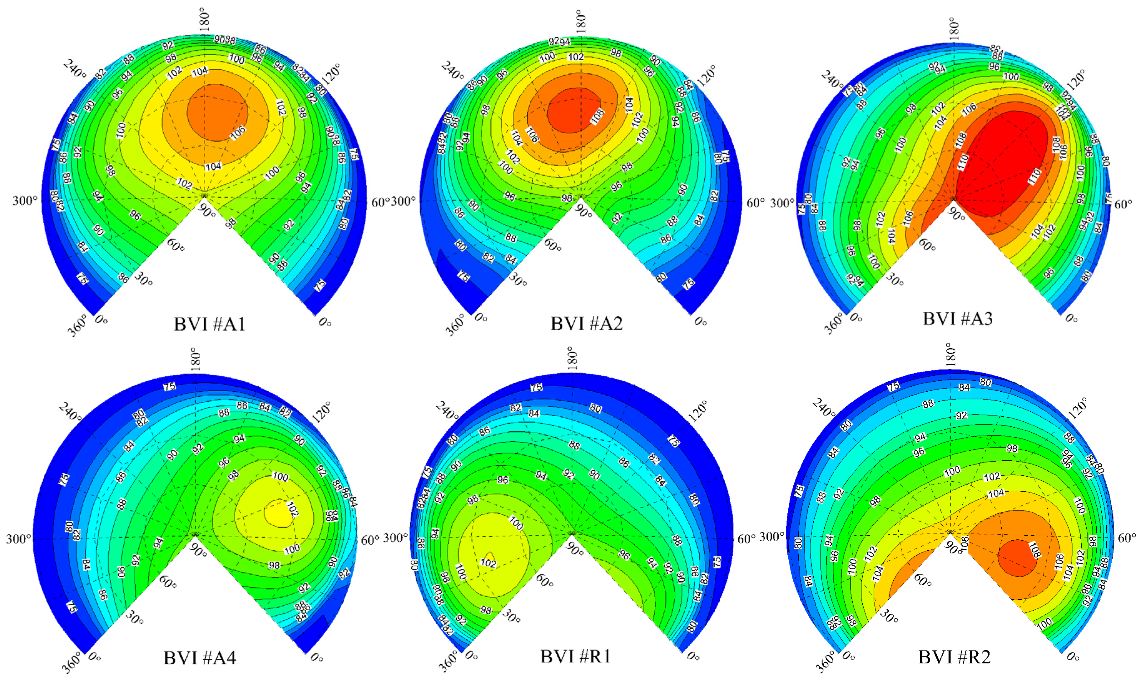
During the calculation of BVI noise, the surface blade load is stored along the azimuth angle at each spanwise location. The impulsive surface loads from one interaction are extracted, with a smooth processing applied to the impulsive loads from others. The propagation characteristics of six BVIs can be distinguished effectively from each other, and the peak noise level contours on the 3.44 R hemi-spherical surface are presented in Figure 8. It is clearly shown that the noise from each interaction has a definite radiation direction and noise intensity, which determines the spatial occurrence of acoustic “hotspots.” Interactions #A1 and #R1 are oblique interactions, the noise from which radiates to around 160° and 325° in azimuth and about 40° below the rotor plane, respectively. Despite the small miss-distance of #A1 and #R1, the interaction angle changes with the azimuth angle during the interaction process, which causes the offset of the generated noise phase, thus the noise intensity is not strong. By contrast, interaction #A3 is a parallel interaction as well as #R2 at the tip of the blade, inducing a strong impulsive effect that causes stronger noise. It is also evident that interaction #A3 radiating to around 120° in azimuth and 45° below the rotor plane dominates six BVIs, the peak noise level contour of which determines the BVI noise radiation field. In addition, interaction #A2 radiating its acoustic energy to 170–200° in azimuth down the rotor is stronger than #A1 but weaker than #A3 in noise intensity because of the fact that the wake angle, the miss-distance, and the interaction angle lie between those of #A1 and #A3. The noise from interaction #A4 is weaker due to the large value of the miss-distance, radiating to 70° in azimuth down the rotor.
3.3. Sensitivity Study of BVI Noise
In this section, the parametric study on the blade airload and BVI noise is investigated. The computational parameters considered are as follows: (1) tip-path-plane angle; (2) thrust coefficient; (3) tip Mach number; (4) advance ratio. The baseline of the computational parameters of , , , and is used for all further cases, unless otherwise stated.
3.3.1. Tip-Path-Plane Angle
The BVI airload and noise characteristics at five tip-path-plane angles varied from −2° to 3° (negative tilted forward) have been discussed with , , and Matip kept constant.
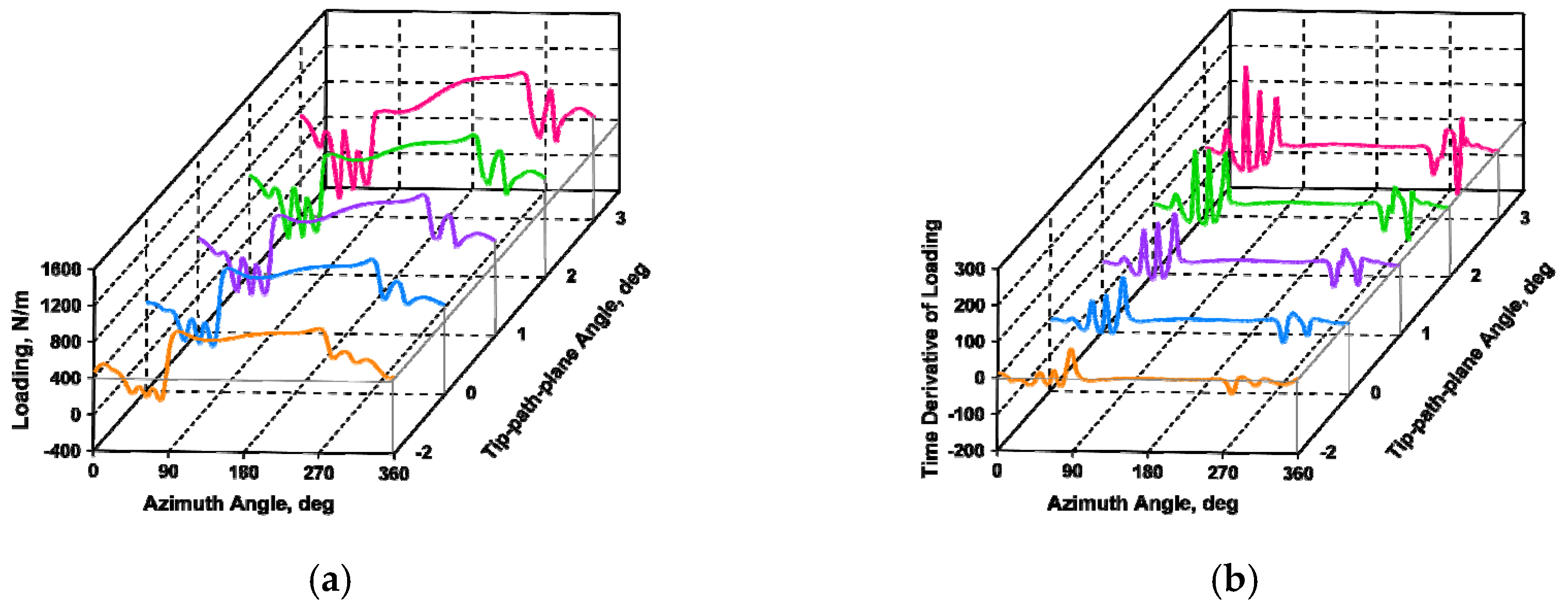
The tip-path-plane angle affects the wake axial movement, making an evident change to the miss-distance. Figure 9 shows the miss-distance varying with the azimuth angle at αtpp = −2°. Compared with the results in Figure 6, the miss-distance increases with a tilted forward angle. We see in Equation (14) that the amplitude of BVI noise depends on the interaction airload and its time derivative, thus the impacts on the sectional airload at 0.9 R are illustrated in Figure 10. As shown, with the rotor disk tilted forward, the impulse load amplitude decreases and the impulse characteristics become weaker due to the increase in the miss-distance.
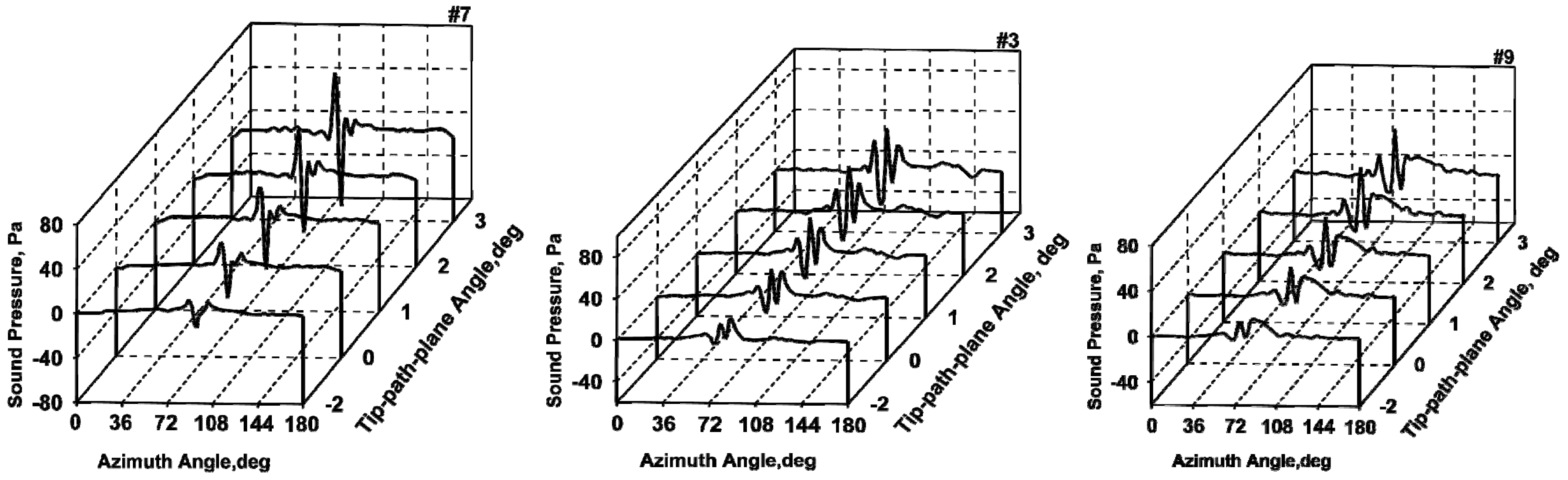
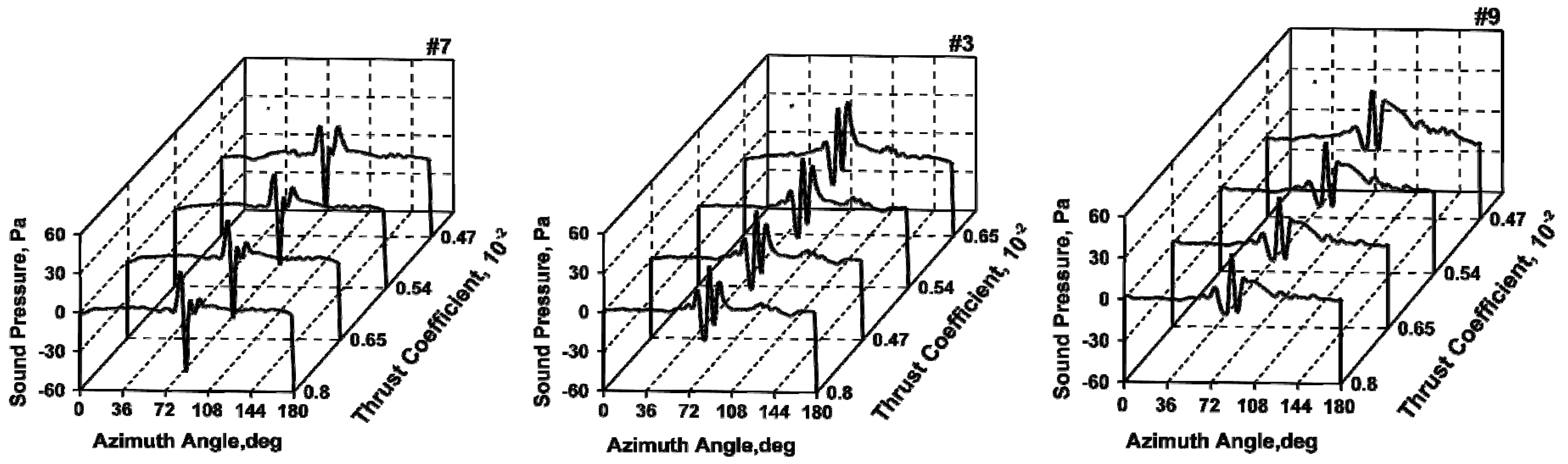
The predicted sound pressure varying with the tip-path-plane angle at #7, #3, and #9 are presented in Figure 11. At each observation location, the sound pressure exhibits similar waveform characteristics at different , the amplitude of which quickly declines with the rotor disk tilted forward due to the increase in the miss-distance. Furthermore, in a strong BVI state, strong impulse characteristics appear, while in a weak BVI state, not only is the noise amplitude small but the frequency is also low.
Figure 12 shows the effects of the tip-path-plane angle on BVI noise directivity. At αtpp = 2°, a high noise level appears at 120° in azimuth and the noise energy is relatively concentrated; this is largely from the parallel interaction #A3 for the small miss-distance. With the rotor disk tilted forward, the BVI noise weakens and the radiation direction is no longer concentrated. At this time, the blade thickness noise becomes more influential, radiating its acoustic energy to the front of the rotor near the rotor plane (Figure 12b).
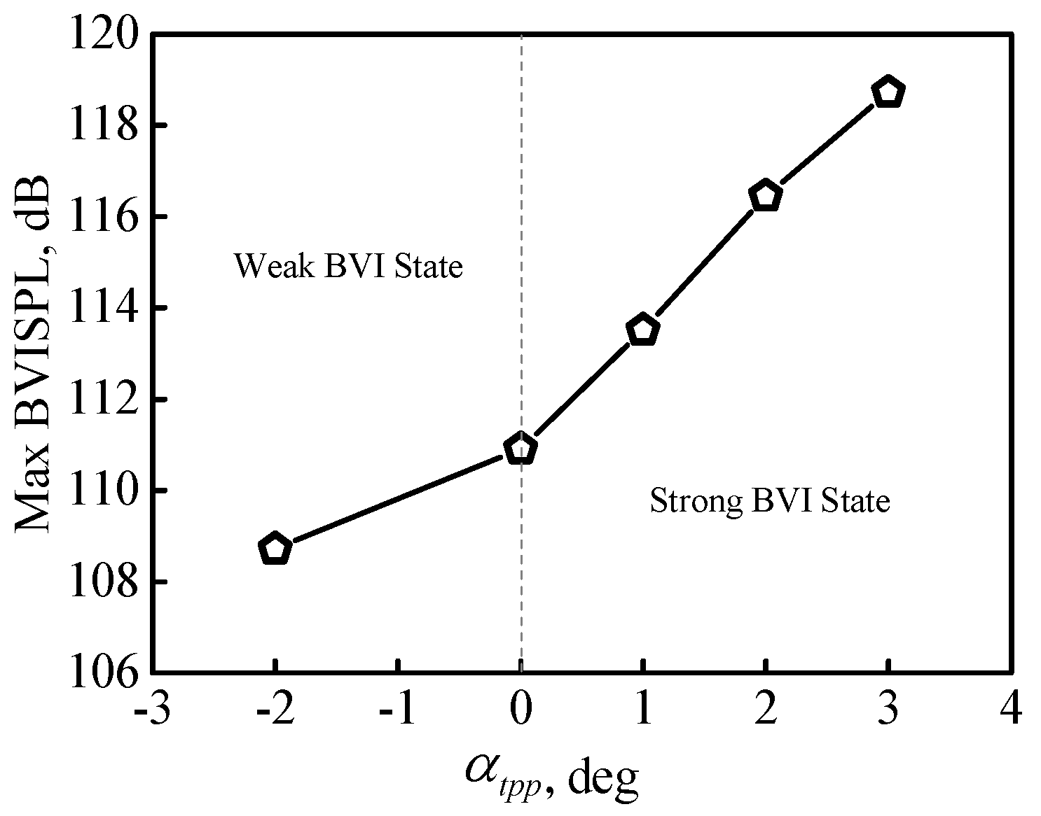
The effects of tip-path-plane angle on the peak BVI noise level are correspondingly shown in Figure 13. When the rotor disk is tilted forward, the peak noise level changes slowly with because the rotational noise dominates the acoustic field. However, when the rotor disk is tilted backward, BVI occurs and the peak noise level changes quickly with . This indicates that the tip-path-plane angle has more influence in the BVI state but less influence in the non-BVI state.
3.3.2. Thrust Coefficient
In this section, by holding the advance ratio, tip-path-plane angle, and tip Mach number constant, we can examine the impact of the thrust coefficient from 0.0047 to 0.0080 on the BVI noise characteristics.
The thrust coefficient impacts the wake-induced downwash but has less impact on the interaction angle. Figure 14 shows the predicted sound pressure at different thrust coefficients at #7, #3, and #9. The sound pressure waveforms at the three observation locations are seen to be less sensitive to the thrust coefficient due to the double effects of vortex strength and miss-distance. On the one hand, the BVI noise increases with the vortex strength, which is proportional to the thrust coefficient. On the other hand, the miss-distance increases with the thrust coefficient, producing reductions in BVI noise.
The contour plots of SPL at two thrust coefficients are compared in Figure 15. At , two peak noise levels appear in space, respectively, from the parallel interaction #A3 and the oblique interaction #A2, which radiates to 180°–240° in azimuth down the rotor. With increasing to 0.0080, interaction #A2 becomes stronger than #A3, and finally dominates the BVI noise propagation. Meanwhile, as the vortex strength influences more strongly than the miss-distance, the BVI noise at is stronger than that at .
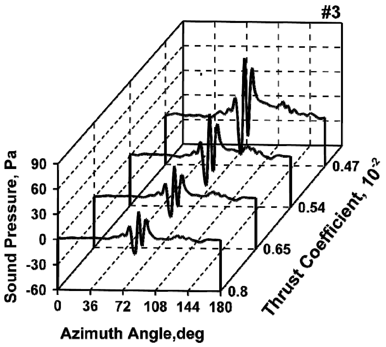
In the above analysis, is kept constant so the miss-distance and vortex strength both make contributions when the thrust coefficient increases. Therefore, another sample trimming to keep the miss-distance constant is provided to analyze the isolated effect of the vortex strength. Figure 16 accordingly presents the predicted sound pressure varying with at #3. Compared with the results in Figure 14, the relative strength of the sound pressure from each interaction is seen to be similar and the amplitude changes proportionately with the thrust coefficient.
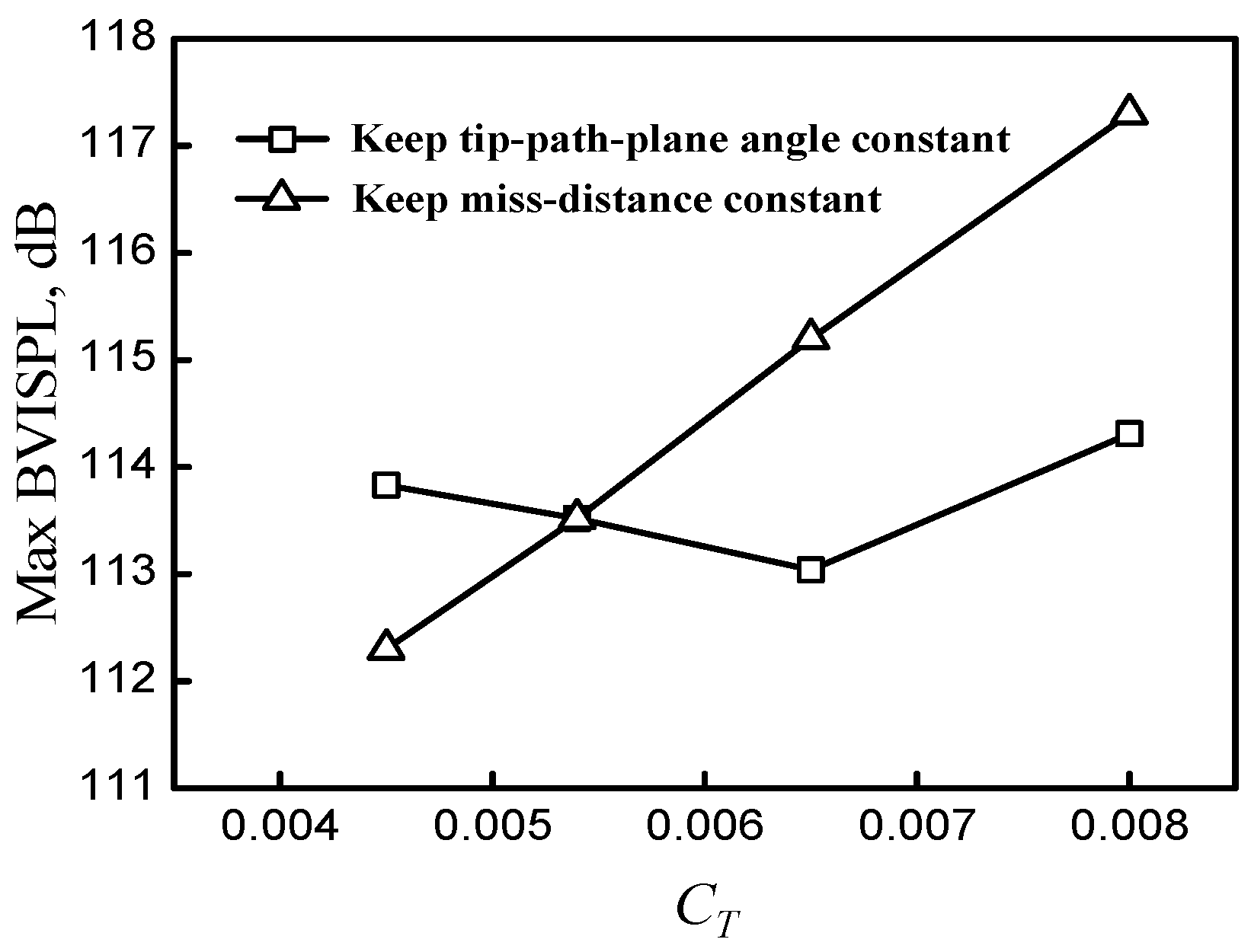
Figure 17 shows the peak BVI noise level varying with the thrust coefficient in different states. If we only consider the impact of vortex strength, the peak noise amplitude is linear to , while if the effects of both vortex strength and miss-distance are considered, the peak noise amplitude seems to be less sensitive to , which means that variation in the thrust coefficient changes the noise propagation, but has little effect on the noise intensity.
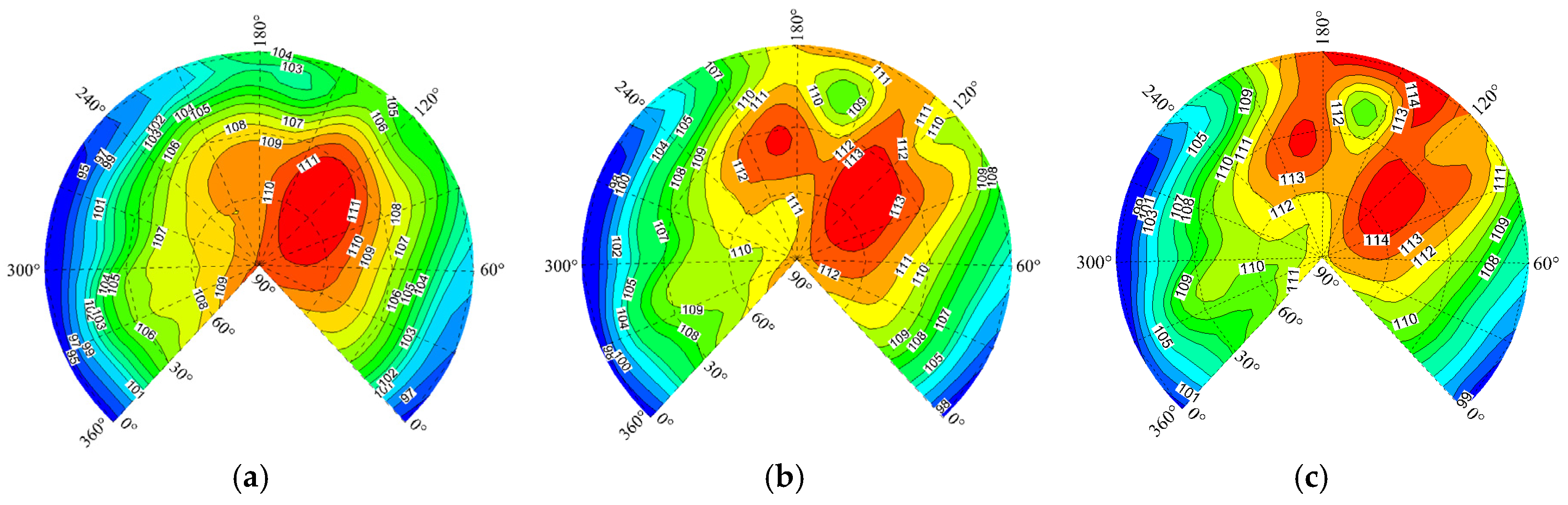
3.3.3. Tip Mach Number
By holding the advance ratio, thrust coefficient, and tip-path-plane angle constant, the tip Mach number increases from 0.55 to 0.725 to analyze the effects on the BVI noise characteristics.
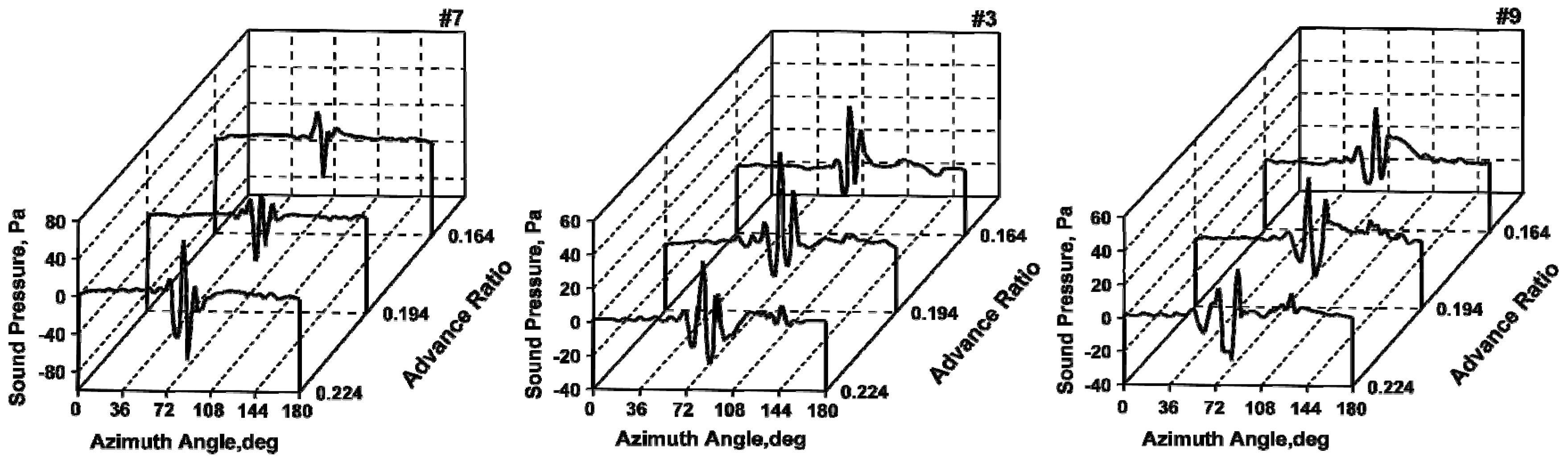
The locations of BVI events on the rotor plane and the miss-distance on the axial plane are less sensitive to Matip because the wake skew angle and the basic epi-cycloid are not affected by Matip. Figure 18 illustrates the sound pressure at #7, #3, and #9 at different tip Mach numbers. With each increasing tip Mach number, the impulse waveform seems unaffected, while the amplitude increases at each observation location. When Matip increases to 0.7, the local Mach number on the advancing side reaches transonic speed, and interactions #A1 and #A2 are more influential which accounts for the stronger noise impulse characteristics. However, it should be noted that the calculation of BVI noise in this paper treats Equations (13) and (14) as linear equations which are nonlinear at transonic speed.
Figure 19 shows the contour plots of SPL for three tip Mach numbers. As Matip increases, interactions #A1 and #A2 become more influential (Figure 19b), and two peaks of sound pressure appear. When the tip Mach number reaches 0.725, one can observe that the BVI noise largely from #A1 and #A2 become stronger; on the other hand, another strong noise which radiates to the rotor plane appears in space.
Figure 20 presents variations in peak noise levels as functions of the tip Mach number. It is observed that 5 dB increases in the maximum BVI noise occur when the tip Mach number varies from 0.55 to 0.725, demonstrating that the tip Mach number is one of the most sensitive governing parameters of BVI noise.
3.3.4. Advance Ratio
To study the effect of the advance ratio, the BVI noise at three BVI states () are simulated with a tip-path-plane, thrust coefficient, and tip Mach number that are all constant.
When the advance ratio changes, the relative motion between the wake and rotor disk dramatically impacts the locations of BVI events and interaction angles; Figure 21 shows the locations of BVI events on the rotor disk at . Compared with the results in Figure 5a, the interaction locations undoubtedly move backward with increasing , and interaction #A2 changes into a parallel interaction.
Figure 22 presents the impact of the advance ratio on the predicted sound pressure at #7, #3, and #9. As #7 is located between the noise level peaks from interactions #A2 and #A3, a negative impulse from #A3 dominates the sound pressure signature at . With increasing , the impulse characteristics increase because interaction #A2 changes to a parallel interaction. However, at the same time the noise radiation direction will move down the rotor disk (Figure 23), which is why the sound pressure at #3 and #9 reach their maximum values at rather than . The conclusion we have drawn from these analyses is that the sound pressure signature at one observation location is closely associated with the dominant interaction in BVI, which generates stronger impulse noise.
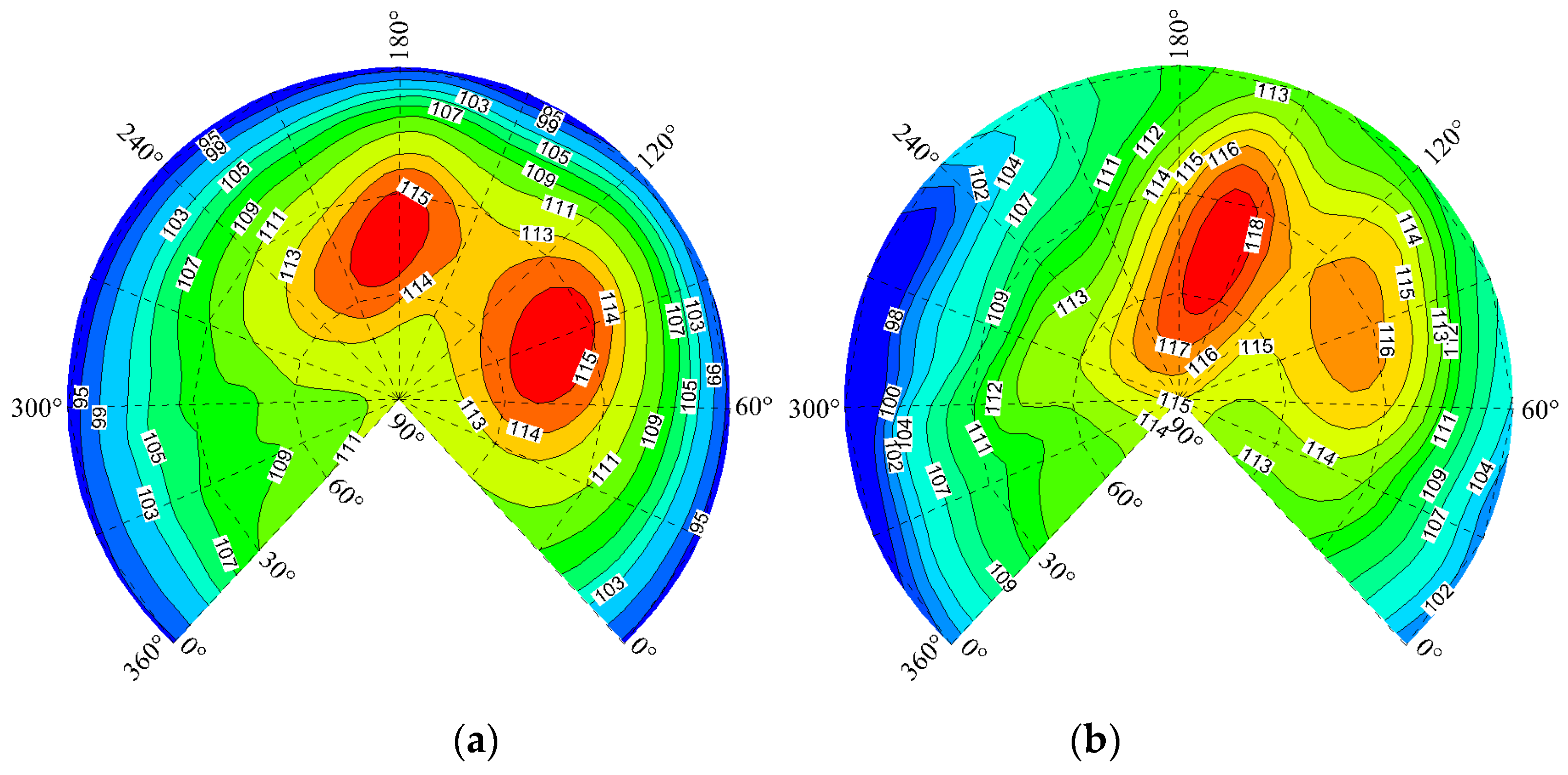
A change in the interaction angle makes a difference in noise directivity. At (Figure 23a), interactions #A2 and #A3 dominate the BVI noise propagation as compared with the radiation direction at . However, when the advance ratio increases to 0.224, the noise from #A2 becomes dominant because the interaction #A2 changes to a parallel interaction. We also observed that the radiation direction of the BVI noise moves down the rotor disk. This agrees with the conclusions of the rotor/isolated vortex line interference instances in which an interaction changes to a parallel interaction, and then the noise radiation direction from it moves down the rotor disk [28].
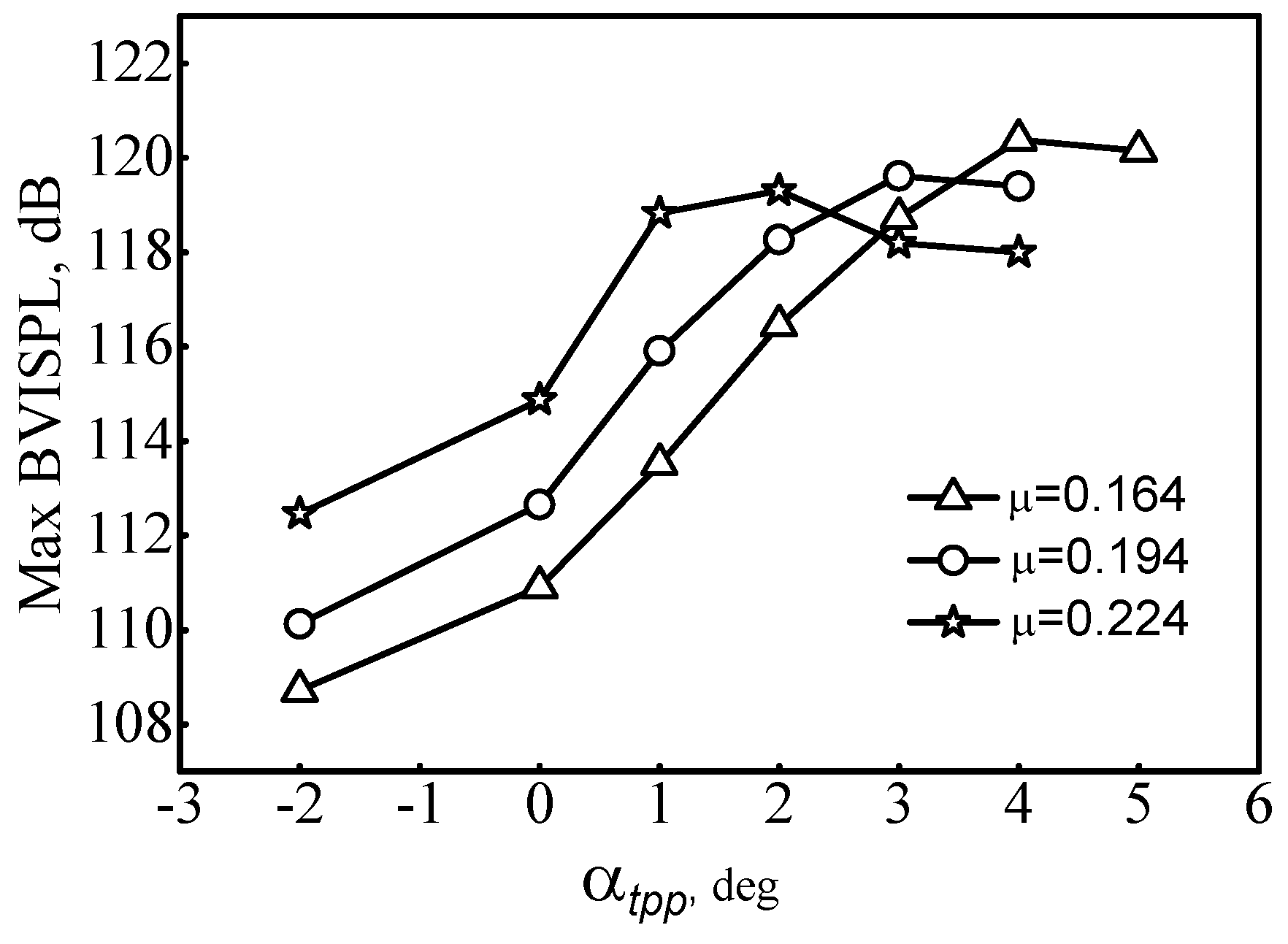
The peak noise level varying with at different advance ratios is presented in Figure 24. At the same tip-path-plane angle, the greater the forward speed is, the stronger the BVI noise will be due to higher noise radiation efficiency on the advancing side. However, with an increasing backward tilt angle, an inflection point appears at ; the explanation for this is that at larger values of , the vortex filament moves faster above the rotor disk, thus the BVI noise decreases earlier for the inverse miss-distance.
4. Conclusions
In this study, a high-resolution coupled method CFD/VWM was adopted to study the aerodynamic characteristics of blade-vortex interaction, and the FW-H equation was utilized to calculate the acoustic characteristics. The BVI condition of the AH-1/OLS rotor was analyzed using the new hybrid method. A parametric study was performed to examine the effects on the BVI airload and noise characteristics. The following conclusions have been drawn from this study:
- (1)
- The rotor wake is an important parameter that contributes to the accuracy of BVI noise prediction. Compared with the CFD/FW-H method, the hybrid CFD/VWM/FW-H method predicts a more accurate rotor wake and the impulsive sound pressure agrees better with the available test data. The hybrid method is also capable of reducing the computation time and resources, given that the computation time is about one-seventh of the CFD/FW-H method.
- (2)
- Variation in the tip-path-plane angle changes the miss-distance, affecting the BVI noise. In a strong BVI state, BVI noise is dominated by the parallel interaction #A3 that radiates to 120° in azimuth and 45° below the rotor plane. With the rotor disk tilted forward, BVI noise becomes weaker, and even disappears due to the reduction in the parallel interaction #A3. Meanwhile, the noise intensity decreases with increases in the miss-distance.
- (3)
- Increases in thrust coefficient oppositely impact the vortex strength and miss-distance, which accounts for the little changes in the sound pressure and the peak noise level. However, the radiation direction of the BVI noise moves from around 120° to 200° in azimuth down the rotor as the oblique interaction #A2 becomes stronger and dominates the BVI noise propagation.
- (4)
- Increasing the tip Mach number has little effect on the interaction angle and miss-distance, but greatly increases the noise radiation efficiency and the dynamic pressure on the advancing side, enhancing interactions #A1 and #A2. Therefore, the BVI noise intensity increases and the radiation directions from #A1 and #A2 become the main propagation direction of BVI noise. When the tip Mach number reaches transonic, BVI noise will never dominate the acoustic field in space.
- (5)
- Increases in the advance ratio greatly changes the interaction azimuth and interaction angle such that the interaction locations move backward and interaction #A2 changes to a parallel interaction. Thus BVI noise dominated by the parallel interaction #A2 radiates to around 160° in azimuth down the rotor. Also, the BVI noise intensity increases provided that the angle of the backward tilt is small. When it is not, the increase in the inverse miss-distance reduces the BVI noise.
- (6)
- Reductions in BVI noise can be obtained by increases in the miss-distance of the parallel interaction with the proper tip-path-plane angle and forward speed adjustment or by decreases in the tip Mach number. Decreases or increases in thrust coefficient change only the propagation direction, not its magnitude.
Acknowledgments
This work was supported by National Natural Science Foundation of China (Grant Number: 11302103).
Author Contributions
Yinyu Zhao, Yongjie Shi and Guohua Xu contributed to the formulation and analysis of BVI noise problem; Yinyu Zhao and Yongjie Shi performed the numerical simulation; Guohua Xu offered useful suggestions for the writing thought; Yinyu Zhao wrote the paper.
Conflicts of Interest
The authors declare no conflict of interest.
Notation
| Sound speed, m/s | |
| Lift coefficient of the blade section | |
| .Rotor thrust coefficient | |
| Energy | |
| Inviscid convective flux vector | |
| f = 0 | Equation of the body surface in motion |
| Viscous flux vector | |
| li | Force/unit area on medium |
| Rotor tip Mach number | |
| Mr | Local Mach number in radiation direction |
| Rotor radius | |
| re | Source-to-observation distance |
| ta | Observation time |
| Velocity field | |
| Free stream velocity | |
| Volume of the pth vortex particle | |
| Relative velocity of the blade section | |
| Conserved variables vector | |
| (x, y, z) vortex particle displacement from the rotor hub center | |
| Vorticity strength | |
| Tip-path-plane angle | |
| Rotor bound circulation | |
| Rotor advance ratio | |
| Kinematic viscosity | |
| Air density | |
| Vorticity field | |
| Non-dimensional vorticity magnitude | |
| Hamiltonian operator | |
| p | Particle index |
| Free stream |
References
- Malovrh, B.; Gandhi, F. Sensitivity of Helicopter Blade-Vortex-Interaction Noise and Vibration to Interaction Parameters. J. Aircr. 2005, 42, 685–697. [Google Scholar] [CrossRef]
- Yu, Y.H. Rotor blade–vortex interaction noise. Prog. Aerosp. Sci. 2000, 36, 97–115. [Google Scholar] [CrossRef]
- Boxwell, D.A.; Splettstoesser, W.R.; Schultz, K.J.; Schmitz, F.H. Helicopter Model Rotor-Blade Vortex Interaction Impulsive Noise: Scalability and Parametric Variations. J. Am. Helicopter Soc. 1987, 32, 5–12. [Google Scholar]
- Yu, Y.H.; Tung, C.; Gallman, J.; Schultz, K.J.; van der Wall, B.; Spiegel, P.; Michea, B. Aerodynamics and Acoustics of Rotor Blade-Vortex Interactions: Analysis Capability and its Validation. In Proceedings of the 15th AIAA Aeroacoustics Conference DLR, Long Beach, CA, USA, 25–27 October 1993. [Google Scholar]
- Chung, K. Numerical predictions of rotorcraft un-steady air-loadings and BVI noise by using a time-marching free-wake and acoustic analogy. In Proceedings of the 31st European Rotorcraft Forum, Florence, Italy, 13–15 September 2005. [Google Scholar]
- Wall, B.G.V.D. Extensions of prescribed wake modelling for helicopter rotor BVI noise investigations. CEAS Aeronaut. J. 2012, 3, 93–115. [Google Scholar] [CrossRef]
- Strawn, R.C.; Caradonna, F.X.; Duque, E.P.N. 30 Years of Rotorcraft Computational Fluid Dynamics Research and Development. J. Am. Helicopter Soc. 2006, 51, 5–21. [Google Scholar] [CrossRef]
- Harris, R.E.; Sheta, E.F.; Habchi, S.D. An Efficient Adaptive Cartesian Vorticity Transport Solver for Vortex-Dominated Flows. AIAA Pap. 2010, 48, 2157–2164. [Google Scholar] [CrossRef]
- Yang, A.; Yang, X. Multigrid Acceleration and Chimera Technique for Viscous Flow Past a Hovering Rotor. J. Aircr. 2015, 48, 713–715. [Google Scholar] [CrossRef]
- Lakshminarayan, V.K.; Kalra, T.S.; Baeder, J.D. Detailed Computational Investigation of a Hovering Microscale Rotor in Ground Effect. AIAA J. 2013, 51, 893–909. [Google Scholar] [CrossRef]
- Gennaretti, M.; Bernardini, G. Novel Boundary Integral Formulation for Blade-Vortex Interaction Aerodynamics of Helicopter Rotors. AIAA J. 2007, 45, 1169–1176. [Google Scholar] [CrossRef]
- Dimanlig, A.; Jayaraman, B.; Lim, J.; Wissink, A. Application of adaptive mesh refinement technique in helios to blade-vortex interaction loading and rotor wakes. In Proceedings of the 68th Annual Forum of the American Helicopter Society, Virginia Beach, VA, USA, 1–3 May 2012. [Google Scholar]
- Fogarty, D.E.; Wibur, M.L.; Sekula, M.K.; Boyd, D.D., Jr. Prediction of BVI noise for an active twist rotor using a loosely coupled CFD/CSD method and comparison to experimental data. In Proceedings of the 68th Annual Forum of the American Helicopter Society, Virginia Beach, VA, USA, 1–3 May 2012. [Google Scholar]
- Biava, M.; Bindolino, G.; Vigevano, L. Single blade computations of helicopter rotors in forward flight. In Proceedings of the 41st Aerospace Sciences Meeting & Exhibit, Reno, NV, USA, 6–9 January 2003. [Google Scholar]
- Shi, Y.; Zhao, Q.; Fang, F.; Xu, G. A New Single-blade Based Hybrid CFD Method for Hovering and Forward-flight Rotor Computation. Chin. J. Aeronaut. 2011, 24, 127–135. [Google Scholar] [CrossRef]
- Hamid, F.; Ahmad, R.P. A New Coupled Free Wake-CFD Method for Calculation of Helicopter Rotor Flow-Field in Hover. J. Aerosp. Technol. Manag. 2014, 6, 129–147. [Google Scholar]
- Wie, S.Y.; Im, D.Y.; Kwon, J.H.; Lee, D.J. Numerical Simulation of Rotor Using Coupled Computational Fluid Dynamics and Free Wake. J. Aircr. 2010, 47, 1167–1177. [Google Scholar] [CrossRef]
- Sugiura, M.; Tanabe, Y.; Sugawara, H. Development of a Hybrid Method of CFD and Prescribed Wake Model for Helicopter BVI Noise Prediction. Trans. Jpn. Soc. Aeronaut. Space Sci. 2013, 27, 343–350. [Google Scholar] [CrossRef]
- Inada, Y.; Yang, C.; Iwanaga, N.; Aoyama, T. Efficient Prediction of BVI Noise Using Euler Solver with Wake Model. In Proceedings of the 1st International Forum on Rotorcraft Multidisciplinary Technology, Seoul, Korea, 15–17 October 2007. [Google Scholar]
- Shi, Y.J.; Xu, G.H.; Wei, P. Rotor wake and flow analysis using a coupled Eulerian–Lagrangian method. Eng. Appl. Comput. Fluid Mech. 2016, 10, 386–404. [Google Scholar] [CrossRef]
- Shi, Y.; Xu, Y.; Xu, G.; Wei, P. A coupling VWM/CFD/CSD method for rotor airload prediction. Chin. J. Aeronaut. 2016, 30, 204–215. [Google Scholar] [CrossRef]
- Farassat, F. Derivation of Formulations 1 and 1A of Farassat; NASA Technical Reports Server (NTRS): Hampton, VA, USA, 2007. [Google Scholar]
- Luo, H.; Baum, J.D.; Löhner, R. A Fast, Matrix-free Implicit Method for Computing Low Mach Number Flows on Unstructured Grids. Int. J. Comput. Fluid Dyn. 2000, 14, 133–157. [Google Scholar] [CrossRef]
- Roe, P.L. Approximate Riemann solvers, parameter vectors, and difference schemes. J. Comput. Phys. 1981, 43, 357–372. [Google Scholar] [CrossRef]
- Cottet, G.H.; Koumoutsakos, P.D. Vortex Methods: Theory and Practice; Cambridge University Press: Cambridge, UK, 2000. [Google Scholar]
- Eldredge, J.D.; Leonard, A.; Colonius, T. A general deterministic treatment of derivatives in particle methods. J. Comput. Phys. 2002, 180, 686–709. [Google Scholar] [CrossRef]
- Sim, B.W.; Schmitz, F.H. Acoustic Phasing and Amplification Effects of Single-Rotor Helicopter Blade-Vortex Interactions. In Proceedings of the 55th Annual Forum of the American Helicopter Society, Montreal, QC, Canada, 25–27 May 1999. [Google Scholar]
- Shi, Y.J.; Zhao, Q.J.; Xu, G.H. An Analytical Study of Parametric Effects on Rotor–Vortex Interaction Noise. J. Proc. IMechE G J. Aerosp. Eng. 2011, 225, 259–268. [Google Scholar] [CrossRef]
Figure 1.
Schematic diagram of the present coupling method.

Figure 2.
Flow chart of the CFD/VWM/FW-H method.
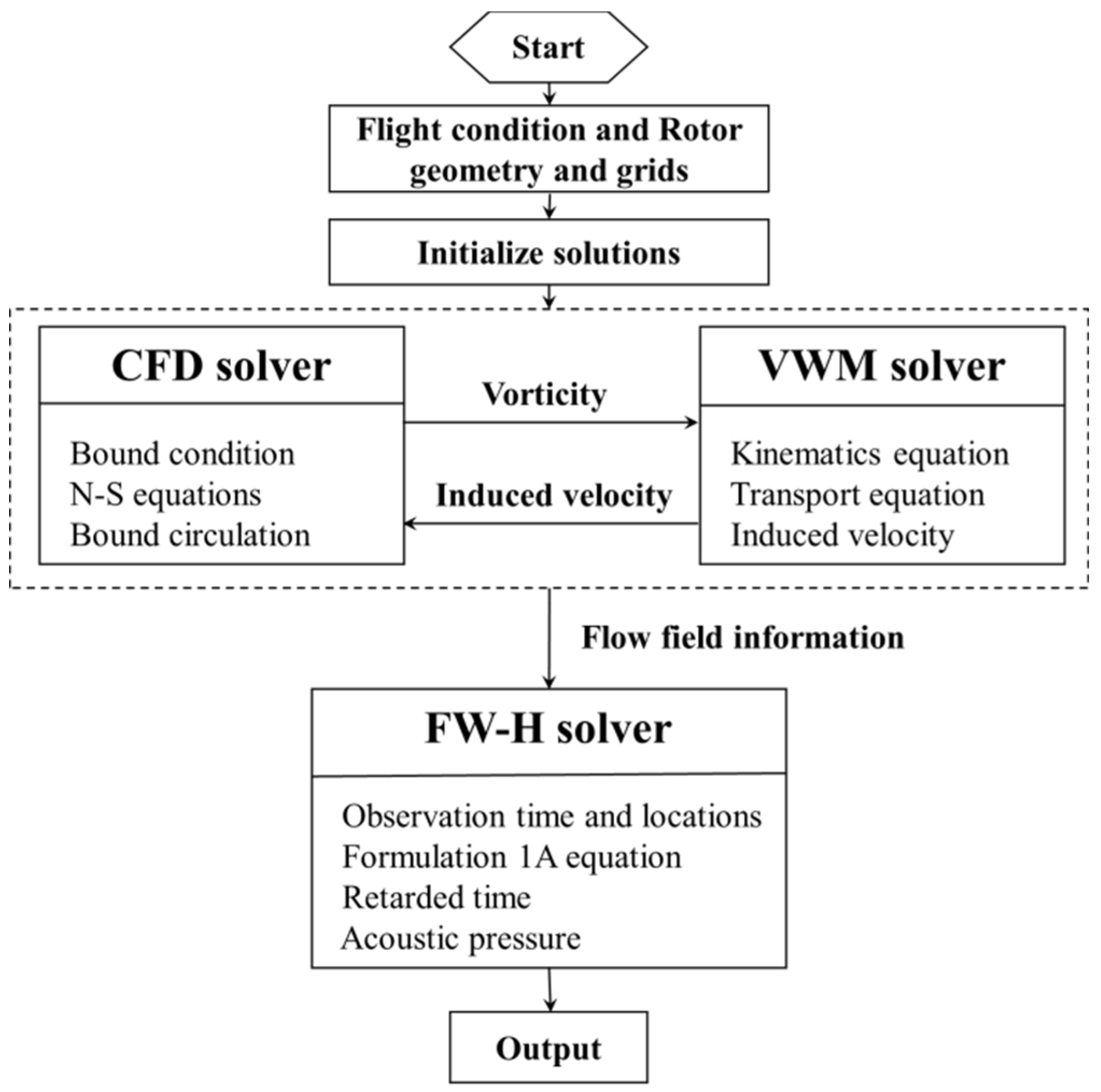
Figure 3.
Observation locations in the OLS model test. (a) Acoustic radiation spherical arc; (b) Lambert projection of spherical arc.
Figure 3.
Observation locations in the OLS model test. (a) Acoustic radiation spherical arc; (b) Lambert projection of spherical arc.

Figure 4.
Predicted rotor wake structure. (a) Full CFD method; (b) CFD/VWM method.

Figure 5.
Locations of BVI events and lift distribution on the rotor disk. (a) BVI events occur on the rotor plane; (b) Lift distribution on the rotor disk.
Figure 5.
Locations of BVI events and lift distribution on the rotor disk. (a) BVI events occur on the rotor plane; (b) Lift distribution on the rotor disk.
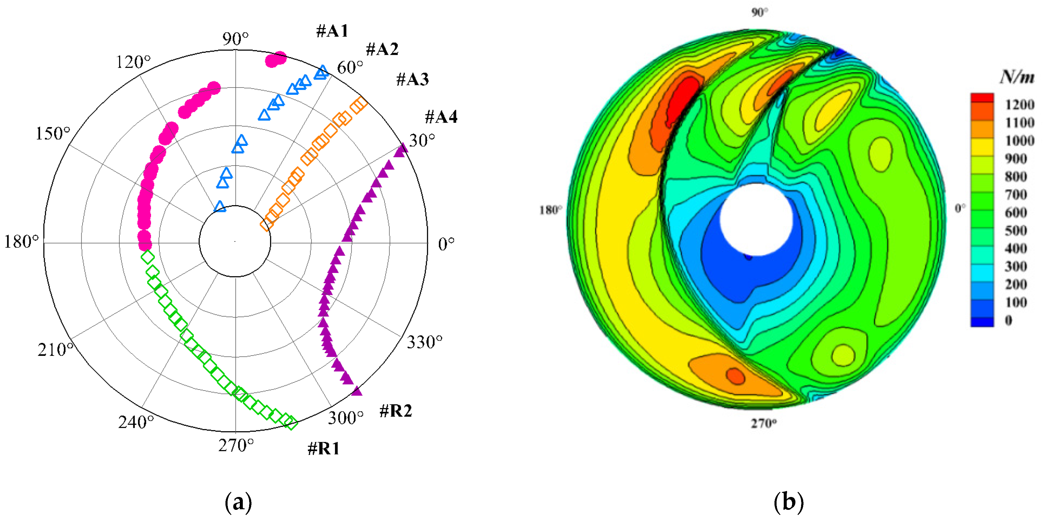
Figure 6.
Miss-distance variance with the azimuth angle.

Figure 7.
Radiation direction and sound pressure signatures of the BVI noise. (a) Contour plot of SPL on the sphere surface; (b) Noise sound pressure at four observation locations.
Figure 7.
Radiation direction and sound pressure signatures of the BVI noise. (a) Contour plot of SPL on the sphere surface; (b) Noise sound pressure at four observation locations.

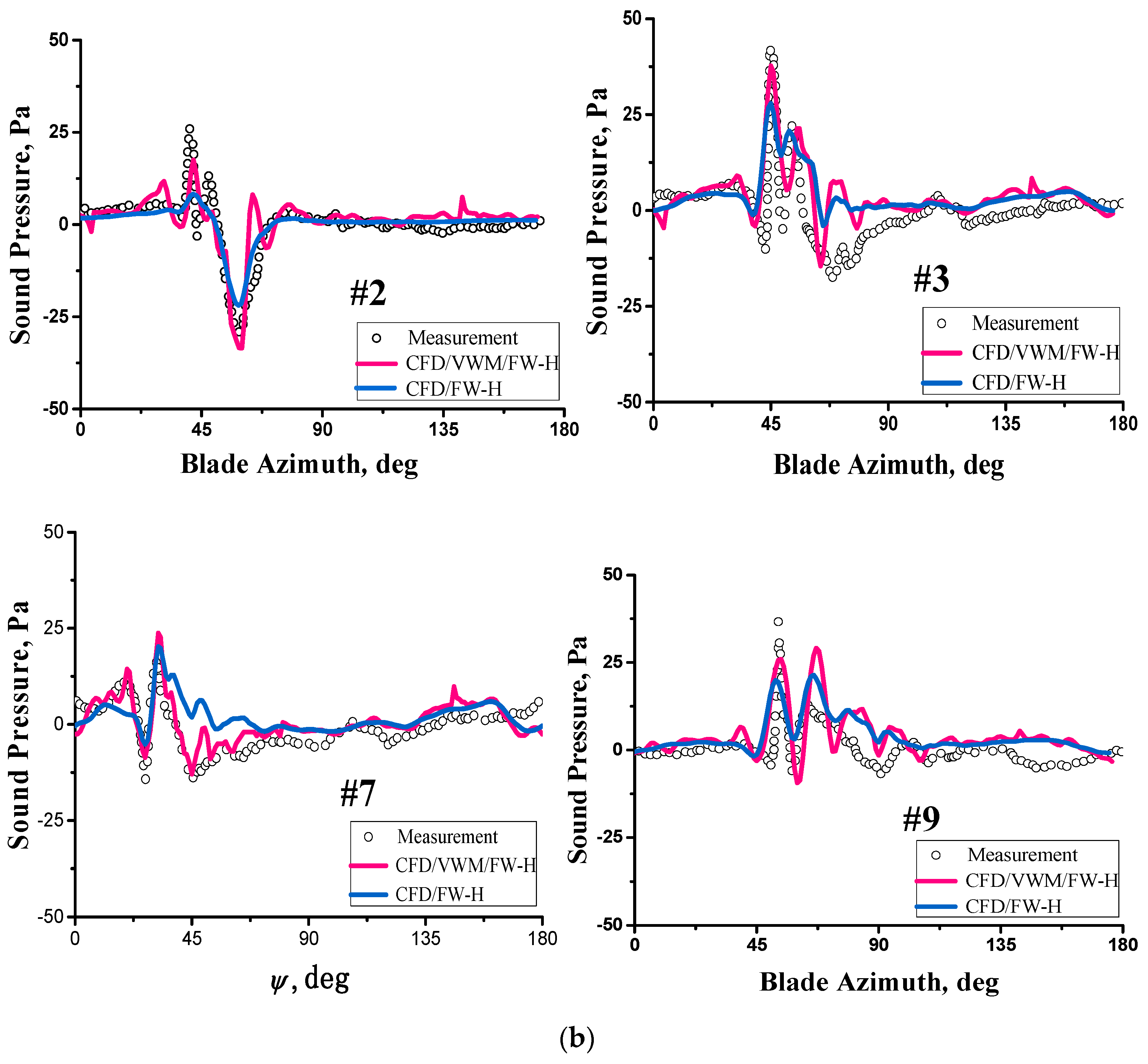
Figure 8.
Peak noise level contours for six BVIs on the sphere surface.

Figure 9.
Miss-distance at αtpp = −2°.
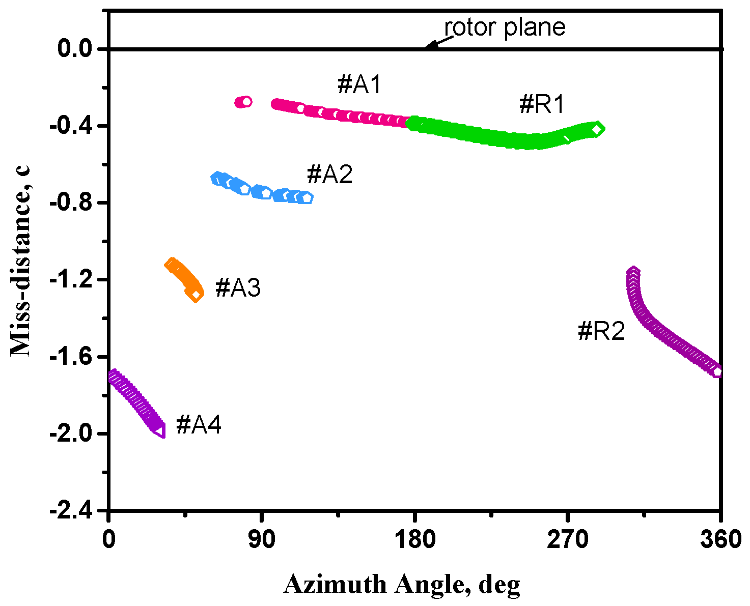
Figure 10.
Sectional airload variance with the tip-path-plane angle at 0.9 R. (a) Loading; (b) Time derivative of loading.
Figure 10.
Sectional airload variance with the tip-path-plane angle at 0.9 R. (a) Loading; (b) Time derivative of loading.

Figure 11.
Predicted acoustic pressure at #7, #3, and #9 variance with the tip-path-plane angle.

Figure 12.
Contour plots of SPL on the sphere surface for different tip-path-plane angles. (a) αtpp = 2°; (b) αtpp = −2°.
Figure 12.
Contour plots of SPL on the sphere surface for different tip-path-plane angles. (a) αtpp = 2°; (b) αtpp = −2°.
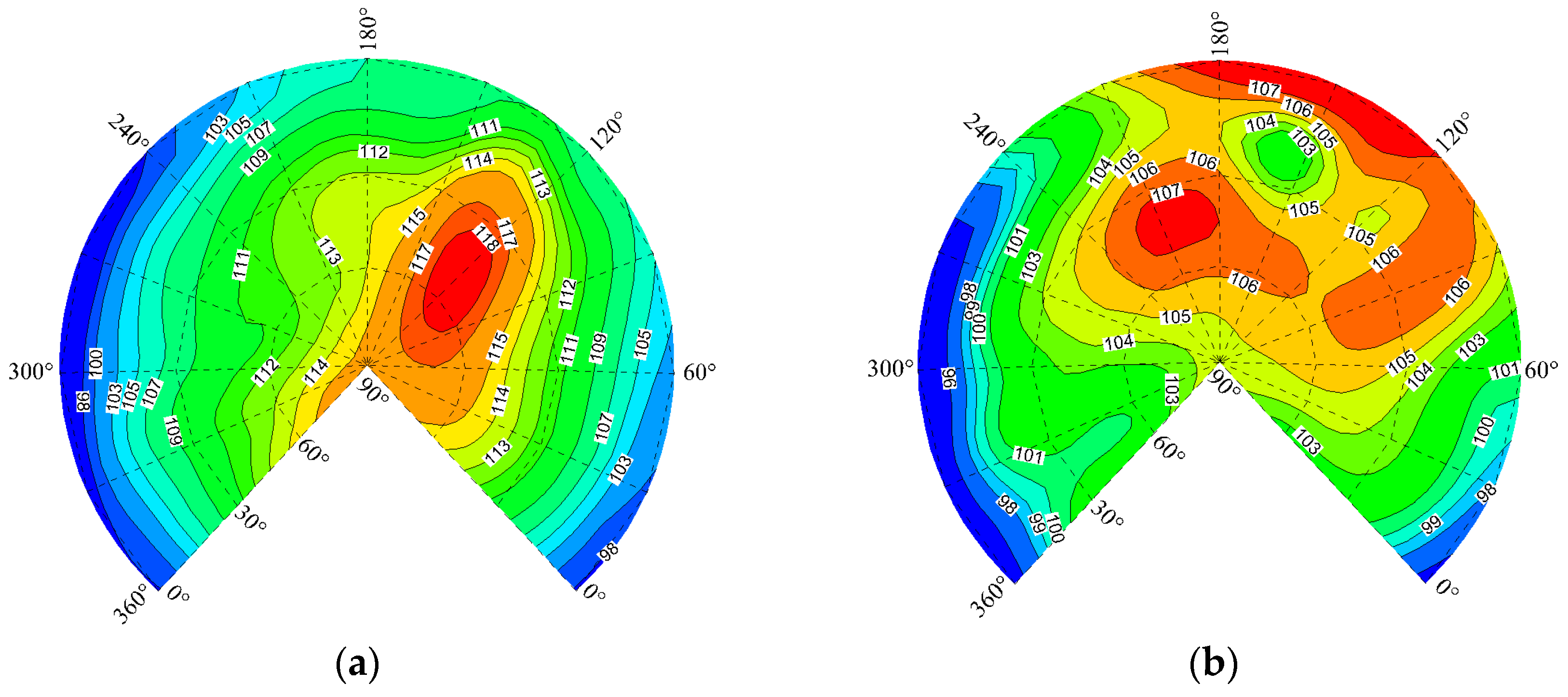
Figure 13.
Max BVISPL variance with the tip-path-plane angle.

Figure 14.
Predicted acoustic pressure at #7, #3, and #9 variance with the thrust coefficients.

Figure 15.
Contour plots of SPL on the sphere surface for different thrust coefficients. (a) ; (b) .
Figure 15.
Contour plots of SPL on the sphere surface for different thrust coefficients. (a) ; (b) .
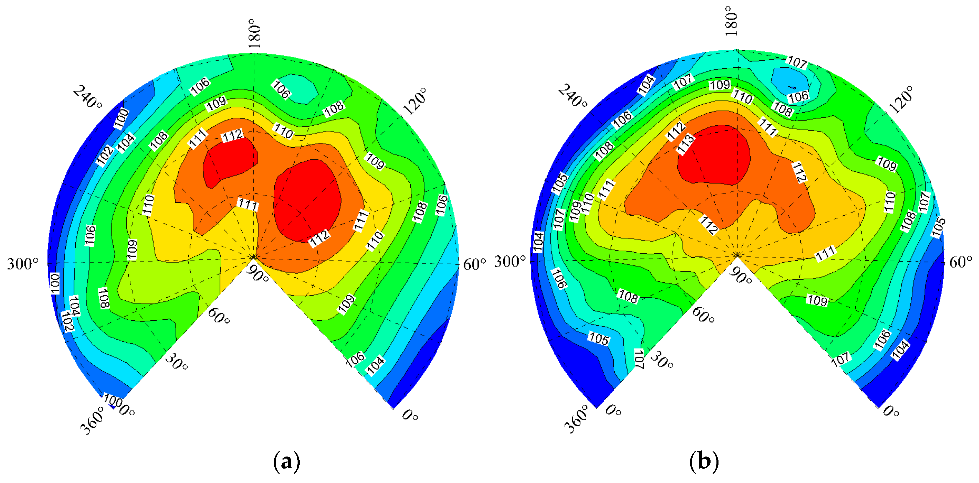
Figure 16.
Predicted acoustic pressure at #3 variance with the thrust coefficients.

Figure 17.
Max BVISPL variance with the thrust coefficient.

Figure 18.
Predicted acoustic pressure at #7, #3, and #9 variance with the tip Mach number.
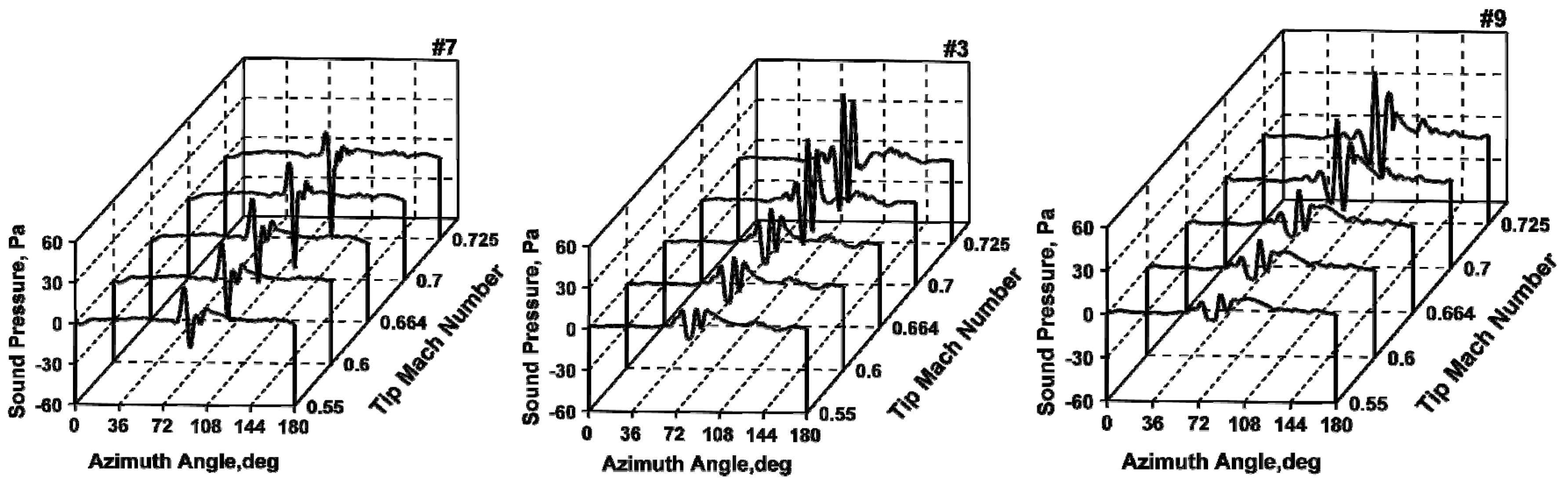
Figure 19.
Contour plots of SPL on the sphere surface for different tip Mach numbers. (a) ; (b) ; (c) .
Figure 19.
Contour plots of SPL on the sphere surface for different tip Mach numbers. (a) ; (b) ; (c) .

Figure 20.
Max BVISPL variance with the tip Mach number.
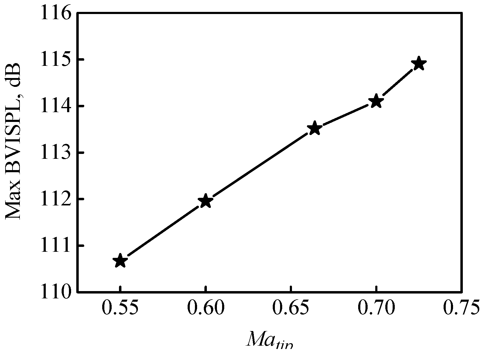
Figure 21.
BVI events occur on the rotor plane at different advance ratios. (a) ; (b) .

Figure 22.
Predicted acoustic pressure at #7, #3, and #9 variance with the advance ratio.

Figure 23.
Contour plots of SPL on the sphere surface for different advance ratios. (a) ; (b) .

Figure 24.
Max BVISPL variance with at different advance ratios.


Table 1.
Control and flapping angles of the OLS rotor for the BVI condition.
| Blade Motion | Blade Collective Pitch | Lateral Cyclic Pitch | Longitudinal Cyclic Pitch | Blade Coning Angle | Longitudinal Flapping Angle | Lateral Flapping Angle |
|---|---|---|---|---|---|---|
| Control Inputs | 6.14° | 0.9° | −1.39° | 0.5° | −1° | 0° |
Table 2.
Numerical condition of the OLS rotor for the BVI condition.
| Numerical Condition | Blade Grid | Number of Blade Aerodynamic Segments | Number of Rotor Revolutions | Time Step Size | |
|---|---|---|---|---|---|
| CFD | VWM | ||||
| Set Values | CO type | 60 | 4 | 6 | 2° |
Table 3.
Comparison of the computation time between the two methods.
| Method | CFD/FW-H Method (Unsteady Solution) | CFD/VWM/FW-H |
|---|---|---|
| Blade grid | ||
| Background grid/particle number | 9,175,040 | 24,439 |
| Total Time | 148 h | 21 h |
© 2017 by the authors. Licensee MDPI, Basel, Switzerland. This article is an open access article distributed under the terms and conditions of the Creative Commons Attribution (CC BY) license (http://creativecommons.org/licenses/by/4.0/).
Share and Cite
MDPI and ACS Style
Zhao, Y.; Shi, Y.; Xu, G. Helicopter Blade-Vortex Interaction Airload and Noise Prediction Using Coupling CFD/VWM Method. Appl. Sci. 2017, 7, 381. https://doi.org/10.3390/app7040381
AMA Style
Zhao Y, Shi Y, Xu G. Helicopter Blade-Vortex Interaction Airload and Noise Prediction Using Coupling CFD/VWM Method. Applied Sciences. 2017; 7(4):381. https://doi.org/10.3390/app7040381
Chicago/Turabian StyleZhao, Yinyu, Yongjie Shi, and Guohua Xu. 2017. "Helicopter Blade-Vortex Interaction Airload and Noise Prediction Using Coupling CFD/VWM Method" Applied Sciences 7, no. 4: 381. https://doi.org/10.3390/app7040381
Note that from the first issue of 2016, this journal uses article numbers instead of page numbers. See further details here.