Flow Measurement by Lateral Resonant Doppler Optical Coherence Tomography in the Spectral Domain


1
Department of Medical Physics and Biomedical Engineering, Faculty of Medicine Carl Gustav Carus, Technische Universität Dresden, 01307 Dresden, Germany
2
Clinical Sensoring and Monitoring, Anesthesiology and Intensive Care Medicine, Faculty of Medicine Carl Gustav Carus, Technische Universität Dresden, 01307 Dresden, Germany
*
Author to whom correspondence should be addressed.
Appl. Sci. 2017, 7(4), 382; https://doi.org/10.3390/app7040382
Submission received: 20 January 2017
/
Revised: 20 March 2017
/
Accepted: 4 April 2017
/
Published: 11 April 2017
(This article belongs to the Special Issue Development and Application of Optical Coherence Tomography (OCT))
Abstract
:In spectral domain optical coherence tomography (SD-OCT), any transverse motion component of a detected obliquely moving sample results in a nonlinear relationship between the Doppler phase shift and the axial sample velocity restricting phase-resolved Doppler OCT (PR-DOCT). The size of the deviation from the linear relation depends on the amount of the transverse velocity component, given by the Doppler angle, and the height of the absolute sample velocity. Especially for very small Doppler angles between the horizontal and flow direction, and high flow velocities, the detected Doppler phase shift approaches a limiting value, making an unambiguous measurement of the axial sample velocity by PR-DOCT impossible. To circumvent this limitation, we propose a new method for resonant Doppler flow quantification in spectral domain OCT, where the scanner movement velocity is matched with the transverse velocity component of the sample motion similar to a tracking shot, where the camera is moved with respect to the sample. Consequently, the influence of the transverse velocity component of the tracked moving particles on the Doppler phase shift is negligible and the linear relation between the phase shift and the axial velocity component can be considered for flow velocity calculations. The proposed method is verified using flow phantoms on the basis of 1% Intralipid solution and diluted human blood.
1. Introduction
Optical coherence tomography (OCT) is a high resolution non-invasive optical imaging modality, which is based on low-coherence interferometry for detecting depth-resolved 2D- and 3D-images of highly scattering semi-transparent samples, e.g., biological tissue [1]. The method uses near-infrared short-coherent light, which is separated within a fiber-coupled or free-space interferometer, to compare the backscattering light from different depth positions within the sample with the reflected light of the reference mirror. Particularly in the early development of the method, the intensity of the interference signal was continuously detected by varying the length of the reference arm to obtain the backscattering light as a function of depth (time domain OCT, TD-OCT). In contrast, the interference signal can be detected in dependence on of the spectral components of the broad band light source (frequency domain OCT, FD-OCT) by a spectrometer configuration (spectral domain OCT, SD-OCT) [2,3,4] or a wavelength-swept source (swept source OCT, SS-OCT) [5,6]. With the emergence of fast line detectors and commercially available stable wavelength-tunable light sources, SD-OCT and SS-OCT became more attractive, since the entire depth information is simultaneously acquired, without any moving reference mirror.
OCT is generally predestined for morphological imaging of biological tissue due to the reconstruction of cross-sectional images (B-scan) and 3D volumetric visualization on the basis of the multiple detected depth scans (so called A-scans in analogy to ultrasound imaging) of the investigated sample. However, functional imaging has become increasingly attractive for the investigation of tissue dynamics and physiology [7,8,9]. This is because the backscattered light not only provides information on the depth-dependent amplitude and phase, but also on physical quantities such as the polarization and the optical frequency shift, which are progressively used for functional tissue imaging. An important enhancement is Doppler OCT (DOCT) for blood flow measurements [10,11]. Most of the proposed Doppler approaches are based on the phase shift between subsequently detected OCT signals, which is widely referred to as phase-resolved Doppler OCT (PR-DOCT) [12,13,14]. For the commonly used spectrometer-based OCT systems, PR-DOCT is still limited by a minimum and ambiguous maximum flow velocity, by interference fringe blurring, due to fast axially moving samples and by a nonlinear relation between the Doppler phase shift and the axial sample velocity for the case of an obliquely moving sample. To increase the dynamic velocity range with high flexibility, Grulkowski et al. have presented adaptive scanning protocols for DOCT, while preserving a high imaging speed [15]. In this work, the Doppler frequency shift related to the phase shift [16] is calculated between consecutive B-scans or segments, instead of subsequent A-scans as has conventionally been employed, resulting in the benefit of mapping low and high flow. To overcome the interference fringe washout for high axial displacement during the A-scan detection time, resonant Doppler imaging was pioneered by Bachmann et al. [17]. This approach uses a moving reference mirror for phase matching the OCT signal by an additional axial reference velocity, to obtain flow-based contrast enhancements of the blood vessels in the OCT images [17,18]. With regard to the nonlinear relationship between the phase shift and axial velocity for an oblique sample movement in SD-OCT [19,20,21], the discrepancy of the assumed linear relation is dramatic in the case of a highly transverse velocity component. Moreover, the measured phase shift always predicts a smaller absolute flow velocity than actually exists. Besides this, the correlation between adjacent A-scans primarily disappears for high transverse velocity components, resulting in a high mean error of the Doppler phase shift [20]. To overcome these limitations for the case of a small Doppler angle between the horizontal direction and the sample velocity, and thereby a highly dominant transverse velocity component, the present approach proposes the matching of the 2D-scanner in the sample arm to the transverse velocity component of the sample motion, comparable to a tracking shot where the camera moves alongside the object to be detected. Consequently, the backscattering signals of the matched oblique sample movement will be highly correlated, whereas those of static sample structures and slowly moving scatterers will be less correlated and damped, depending on the scanner velocity. The method of the so-called lateral resonant Doppler OCT (LR-DOCT) is validated by means of in vitro flow phantom studies with diluted Intralipid and human blood.
2. Phase-Resolved Doppler Model in SD-OCT
2.1. The Relation Between the Doppler Phase Shift and Axial Sample Velocity
The starting point of the phase-resolved Doppler OCT (PR-DOCT) in SD-OCT is the single complex depth scan Γj(z) resulting from the Fourier transform of the detected spectrally shaped interference signal Ij(k,z). This A-scan with index j comprises the amplitude A(z) and the random phase ϕ(z) information of the backscattered light from different depth positions z of the volume scattering sample, as shown by Equation (1):
Here, the amplitude enables the structural imaging, while the phase of a scattering sample relates to a random fluctuation term. Since an axial sample movement between consecutive A-scans separated by the period TA-scan causes a Doppler frequency shift, and with this a phase shift Δϕ(z) of the interference spectrum, the phase information can be used for the measurement of the axial sample velocity vz(z), in consideration of the center wavelength λ0, the refractive index n of the sample, and the time TA-scan needed for one A-scan relating to the sum of the integration time TInt of the line detector of the spectrometer and the detector dead time ΔT due to a possible operating shutter control [21].
The bias-free Doppler phase shift Δϕ(z) is calculated by the multiplication of the complex Fourier coefficient of one A-scan Γj+1(z) and the previous conjugate complex measurement Γj*(z) [20,22], where the resulting complex data contains the Doppler phase shift Δϕ(z) as the argument:
Since the noise of the Doppler phase shift increases with the amount of transverse displacement in the case of an oblique sample motion [19,20], low signal-to-noise ratio (SNR) [16], and detector dead time [21], the amplitude weighted averaging by Equation (4) is recommended.
The discrepancy of the relationship of Δϕ(z) and vz(z) for any oblique sample motion detected with spectrometer-based OCT systems has been theoretically described in detail in previous studies [19,20,21]. To summarize the general description of the Doppler phase shift Δϕ independent of the OCT system parameters, dimensionless coordinates are used as follows:
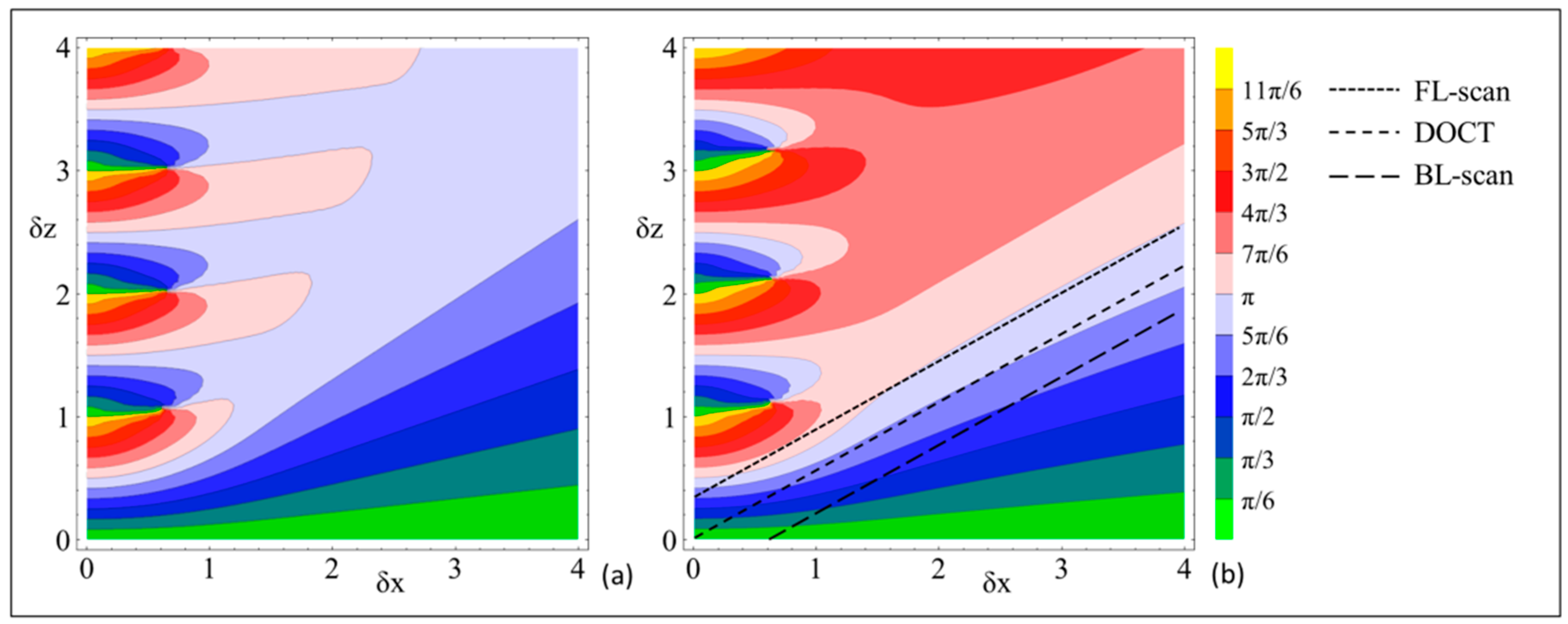
where w0 corresponds to the width of the Gaussian sample beam (FWHM) of the OCT system. Since the dependence of Δϕ on δz and δx cannot be calculated in an analytical way [19,20,21], the numerical result is given by a universal contour plot, where Δϕ is drawn in steps of π/6 for δz and δx ranging from zero to four. Additionally, Δϕ is limited to its principle value between 0 and 2π, for which reason phase shifts exceeding 2π are simply wrapped.
For the case of no detector dead time ΔT/TA-scan = 0, the numerically determined Δϕ is shown by the contour plot in Figure 1a [20]. By considering a partial duty cycle [21] with ΔT/TA-scan = 0.05, as for the system used in this study, Δϕ as a function of δx and δz is changed as presented in Figure 1b. The phase shift Δϕ arisen from an obliquely moving sample with the Doppler angle ϑ, between the x-direction and the sample velocity, corresponds to a linear slope through the origin δx = δz = 0, as exemplarily shown by the central dashed line. The angle ϑ′ in Figure 1, defined as the angle against the horizontal, may not equate with the real world angle ϑ of the experimental setup:
2.2. The Impact of Lateral Resonant Scanning on PR-DOCT
Since the phase-resolved Doppler measurements in SD-OCT are limited for strong transverse components and high sample velocities, the transverse tracking of the obliquely moving sample is proposed in this research and defined as lateral resonant scanning. With this, the impact of the transverse motion component on the Doppler phase shift can be theoretically reduced. For a better comprehension of the subsequent experimental results, a simple geometric model is defined on the basis of Figure 2 for the Doppler measurement in SD-OCT. As shown, a Gaussian sample beam and an oblique sample motion with an arbitrary Doppler angle ϑ are assumed. In this case, a group of scattering particles is supposed to be seen at the end of the detection intervals, [T1, T1 + TInt], [T2, T2 + TInt], and [T3, T3 + TInt], of three consecutive A-scans, where the respective position of the particles is shown by three blue distances and labeled with I, II, and III. Three cases of Doppler measurement performance are drawn in Figure 2: (a) with a static sample beam, resulting in a conventional M-scan (time-resolved A-scan); (b) with a laterally moving sample beam in the direction of the sample movement, resulting in a so-called forward lateral scan (FL-scan); and (c) with lateral scanning in the opposite direction, so-called backward lateral scan (BL-scan). Case (a) corresponds to the common phase-resolved Doppler measurement without imaging, where the sample beam of the OCT system is static to guarantee the highest phase correlation between adjacent A-scans. Due to the limited Gaussian sample beam, the group of particles seen in the time interval [T1, T1 + TInt] are only partly detectable in the subsequent time interval [T2, T2 + TInt] (shown by the red dotted lines), for which reason the measured axial displacement Δzd and Δϕ are reduced, especially for small Doppler angles and large transverse displacements [19,20,21].
Case (b) shows the lateral scanning towards the sample movement, where the sample beam in gray represents the position at T1 + TInt and the one drawn in green shows the position at T2 + TInt. Since the scanner velocity is matched to the transverse velocity of the moving sample, the group of particles detected at time point T1 + TInt is tracked over the entire A-scan time TA-scan, until T2 + TInt. For a temporally invariable sample, the detected movement is purely axial, for which the Δϕ-vz-relation will be linear and the absolute sample velocity can be linearly calculated (cp. Equation (2)). For case (c) of the backward scanning, no phase correlation seems to exist, because the scattering particles detected at T1 + TInt within the gray sample beam are not detectable at T2 + TInt within the green one. Due to the continuous movement of the scanner and the gradual movement of the scattering particles out of the scanning sample beam within TA-scan, a strongly reduced phase correlation exists, leading to a strongly reduced Δz and a significantly decreased Δϕ.
Considering the contour plots in Figure 1 describing the Doppler phase shift in dependence on the normalized axial δz and transverse δx displacement, a lateral resonant scanning relative to the transverse component of the oblique sample movement results in a negative offset in the δx-direction of the linear slope, describing the phase shift. Knowing the Doppler angle ϑ from 2D or 3D scans, the absolute sample velocity can be calculated by the linear Δϕ-vz-relation in Equation (2). Finally, the question of whether LR-DOCT is practicable for moving volume scatterers arises. The challenge for flowing emulsions and suspensions with scattering structures for the near-infrared wavelength range is the temporal variability of the particle position within flow channels or blood vessels, which hampers the particle tracking and LR-DOCT. The experimental validation of this question is the subject of the presented research study.
3. Material and Methods
3.1. OCT System Setup and In Vitro Flow Phantom
In the present study, the 1250 nm wavelength band of the dualband spectral domain OCT system of our workgroup is used [23]. This system contains a commercially available supercontinuum laser light source (SuperK Versa Super Continuum Source, Koheras A/S, Birkerød, Denmark), where the wavelength band with a center wavelength λ0 of 1250 nm has a spectral width Δλ of 200 nm and an axial resolution of 5.3 µm in air. The system comes with a 3D-scanner, whose Gaussian sample beam has a theoretically calculated width of w0 = 9.3 µm in the focal plane and a Rayleigh length of about 200 µm. The scanning unit for 2D-beam deflection at the sample surface is realized by two galvanometer scanners (cp. Figure 3). The system allows 3D-imaging with an A-scan rate of up to 47 kHz. For high backscattering signals with a strong signal-to-noise ratio (SNR) of the sample, the A-scan rate is set to fA-scan = 12 kHz for the flow measurement. The control of the system, the data acquisition and the processing is realized by means of a personal computer and custom software developed with LabVIEW® (National Instruments, Inc., Austin, TX, USA).
LR-DOCT is experimentally validated by a flow phantom consisting of a flow-controlled infusion pump, a glass capillary with a 312 µm inner diameter, and a tubing system to connect both components. The pumped fluids are a 1% Intralipid emulsion as an established flow phantom model for OCT with well-known flow characteristics, and diluted human blood. Here, the fresh human blood of a young healthy volunteer was extracorporeally stabilized with anticoagulant citrate dextrose solution (ACD-A) and diluted with a solution of 6% dextrose and 0.9% sodium chloride in distillated water with a ratio of 1:2, resulting in a hematocrit of ~15%. Despite the enhanced penetration depth into the blood vessels due to the low absorption of hemoglobin and the reduced scattering in the 1250 nm wavelength band, only the dilution enables the lateral resonant flow measurement over the entire capillary lumen of 312 µm, which is comparable to the inner blood vessel diameter of the in vivo mouse model used in our cooperative research [24,25,26]. To avoid sedimentation of the solid blood components and to guarantee a homogenous dispersion of erythrocytes within the capillary, a drop distance was installed within the tubing system in front of the capillary entry, in accordance with the schematic drawing in Figure 3. For the 1% Intralipid sample, the flow rate is set to 9.5 mL/h, corresponding to a peak center velocity of about 69 mm/s, and for the diluted human blood, the chosen flow rate is 8 mL/h, resulting in a center flow velocity of about 62 mm/s, which conforms well to the maximum flow velocity of the saphenous artery of an anesthetized mouse during the systole prevalent in our research project [24]. For the analysis of the velocity values, a parabolic flow profile was assumed because the capillary had a length of 80 mm, the inlet path was considered, and the Reynolds number was less than ten for both samples. The Doppler angle ϑ of 1.7° was measured by taking a volume scan with the 3D-scanner.
3.2. Bi-Directional Lateral Scanning Protocol and Image Correction for Doppler Analysis
The two galvanometer scanners integrated in the scanning unit are controlled by custom developed software based on LabVIEW® (National Instruments, Inc., Austin, TX, USA), with which arbitrary 2D-scanning patterns along the sample surface are realizable. Conventionally, the orthogonally driven X- and Y-galvanometer scanners are controlled for 2D-beam deflection, to allow 3D-imaging. The corresponding scanning protocol can be found in Figure 4a, where B-scans consisting of an arbitrary number of A-scans are detected by the lateral fast scanning Y-scanner and are spatially separated by the X-scanner. The resulting orthogonally running cross section and longitudinal section of the exemplary glass capillary with flowing 1% Intralipid are presented in Figure 4b.
The modified scan protocol for LR-DOCT is shown in Figure 4d. The first of the three B-scans with the stationary Y-scanner is an M-scan, and within the second B-scan, the X-scanner is driven along the moving direction of the sample (forward lateral scan, FL-scan). The third B-scan implies the reversely driven X-scanner (backward lateral scan, BL-scan). The resulting M- and lateral resonant B-mode images, each consisting of 512 A-scans, detected close to the capillary center with fA-scan = 12 kHz and a detector dead time ΔT/TA-scan of 0.05, are presented in Figure 4e. For the FL-scan, the X-scanner was lateral resonantly driven to the flowing oil particles of the 1% Intralipid emulsion at the capillary center.
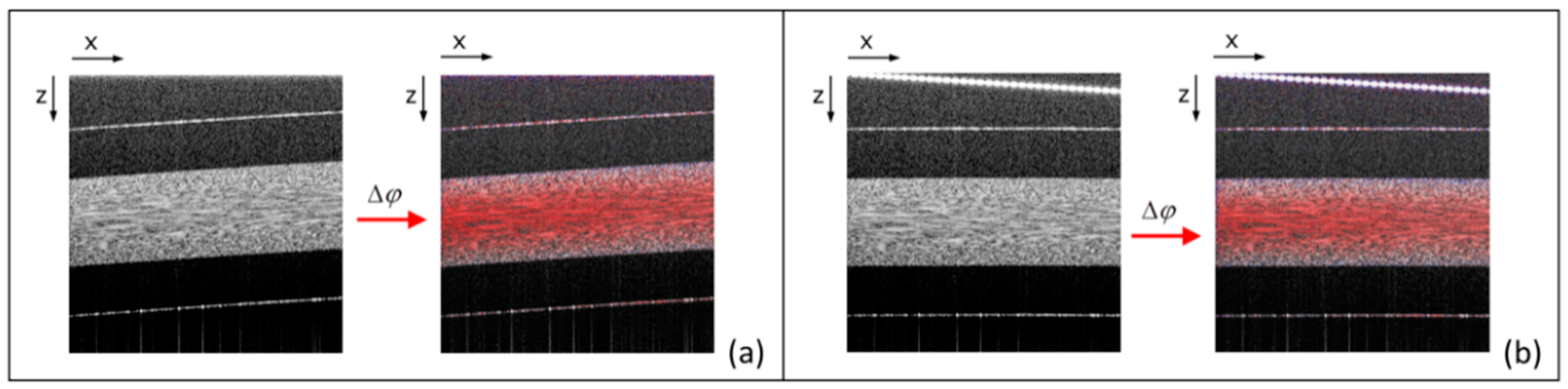
The result of the Doppler analysis by Equation (3) is presented in Figure 5a for the FL-scan of the glass capillary with flowing 1% Intralipid. The calculated Doppler phase shifts are overlaid to the structural information. As the obliquely running direction of the sample hampers the averaging of phase shifts in x-direction, consecutive A-scans are shifted in the z-direction by introducing a k-dependent phase shift. This correction is demonstrated in Figure 5b, using the example of the FL-scan. In analogy to the first shift theorem of the Fourier transform, an additional phase ϕshifted(k,j) is inserted into the real-valued interferometric signal Ij(k,z), as shown in Equation (7). According to Equation (8), the fractional shift of each interference spectrum of the lateral resonant scan corresponds to the tangent of the Doppler angle ϑ, where N is the number of points of the Fourier transformation (FT). With this, the originally obliquely running direction of the capillary, and consequently, the Doppler phase shift due to the fast laterally moving X-scanner across the oblique surface of the glass capillary, are eliminated.
Further processing is identical to the conventional OCT and Doppler OCT processing: a Fourier transform is applied to Ishifted,j(k,z) in accordance with Equation (1) and the Doppler phase shift Δϕ is calculated by multiplying a complex A-scan with the conjugate complex one (cp. Equation (3)).
4. Experimental Results
4.1. LR-DOCT with 1% Intralipid Flow
In order to validate LR-DOCT for moving volume scatterers, Doppler flow experiments are performed by means of a 1% Intralipid emulsion flowing through a glass capillary, as described in Section 3.1. The Doppler angle is 1.7° and the maximum flow velocity at the capillary center is estimated to be 69 mm/s. Thus, the transverse displacement δx of the flowing oil particles of the Intralipid emulsion amounts to 0.6 for the case of the detected M-scan, which strongly reduces the phase correlation [20,21,27].
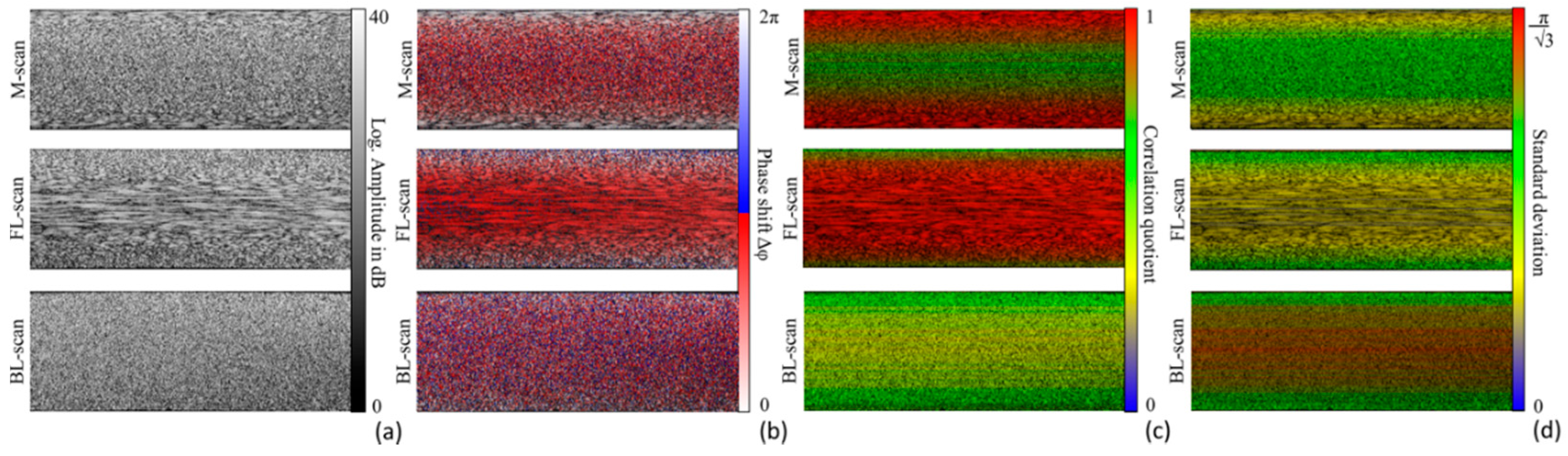
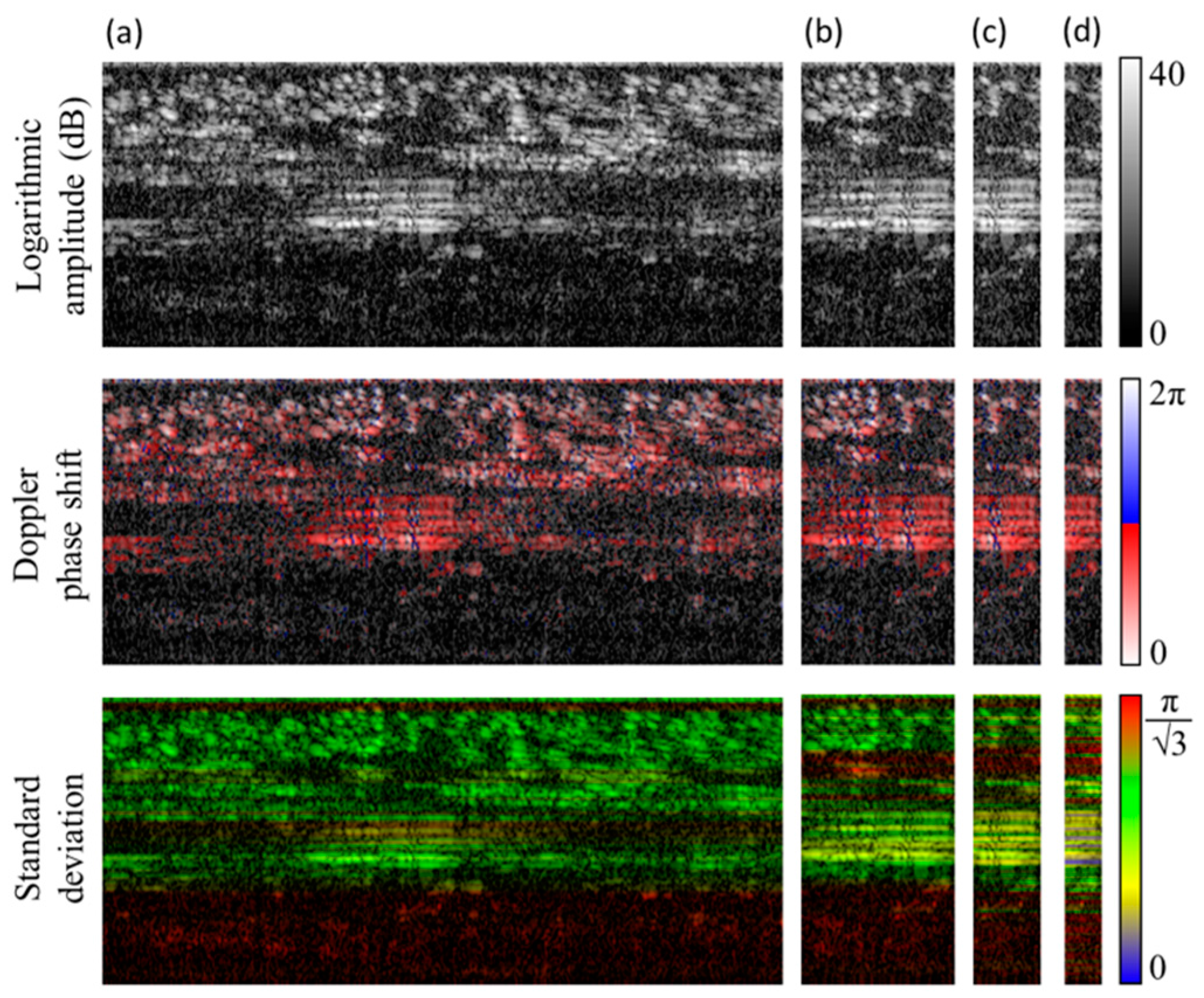
Figure 6 presents the processed flow-relevant parts of the grayscale structural (a) and the Doppler flow images (b) of the detected M-scan, the forward lateral (FL) and the backward lateral (BL) B-scans differing in the speckle pattern, and the resulting Doppler phase shift. The number of analyzed A-scans is chosen to be 512. As expected, highly correlated speckle appears at the capillary border for the M-scan due to the small flow velocity in this area. For the FL-scan, the X-galvanometer scanner velocity is set to 69 mm/s, which corresponds to the transverse velocity component of the Intralipid flow at the capillary center. In this case, the correlation at the border area gets lost, whereas a high correlation occurs at a wide range of the capillary lumen identified by the elongated speckle pattern. In contrast, the speckle seems to be uncorrelated for the case of the BL-scan, where the X-scanner is moved in the opposite direction at 69 mm/s.
The visual assessment of the Doppler images in Figure 6b suggests a high noise of the Doppler phase shift at the capillary center in the M-scan, at the capillary border in the FL-scan, and over the entire capillary lumen in the BL-scan, which is caused by the reduced correlation of adjacent A-scans. As predicted in Section 2.2, the phase-sensitive image of the BL-scan visually shows the highest noise of the Doppler phase shift. For the quantification of the phase correlation, the correlation quotient CQ, defined in former research [20,21], is calculated as a function of z and is overlaid in color on the structural images, as presented in Figure 6c. CQ is shown in red for the highest correlation between consecutive A-scans. The results of CQ prove the suggestions made by the observed speckle patterns in Figure 6a and the estimated phase shift noise in Figure 6b. Additionally, the standard deviation of the mean Doppler phase shift is given in Figure 6d. As described in previous studies [20,21,27], the distribution of Δϕ cannot be worse than isotropic in the original interval of [−π, π], resulting in an upper limit of π/√3, as shown by the red color of the σΔϕ scale bar. By means of the colored structural information for visualizing Δϕ, CQ, and σΔϕ, the possibility to laterally track the flowing oil particles with a simultaneous decrease of the phase shift noise for small Doppler angles and high flow velocities, becomes apparent.
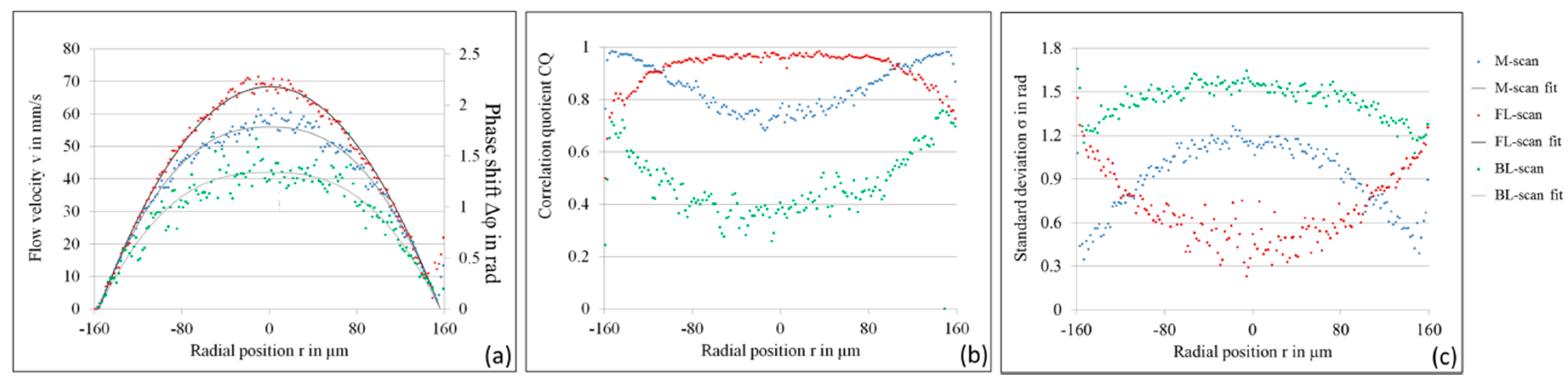
For quantitative analysis, the averaged phase shift of 512 single measurement points is calculated, as described in Equation (4) and presented in Figure 7a. The measured Δϕ of the M-scan shown by the blue points does not display a quadratic profile, verified by the fitted power law with an exponent of 2.4. The Doppler phase shift at the capillary center is measured to be 1.9 rad, which conforms well to the estimation by means of the contour plot in Figure 1b and the transformed Doppler angle ϑ′ of 29°. The result of the forward lateral scan (FL-scan) presented by the red points conforms to a quadratic parabolic profile, with the expected maximum velocity of 69 mm/s at the capillary center. In spite of the increased phase noise at the upper and lower capillary borders, the Doppler phase shift of the tracked Intralipid particles is not limited, and consequently, is truly measured by the linear relation between Δϕ and vz referred to in Equation (2). The non-resonant imaging at the border of the capillary has no influence on the shape. For the backward lateral scan, the flow profile seems to be a flattened plug profile with a fitted exponent of the power law of 2.6. Despite the strongly increased phase noise σΔϕ, an erroneous mean velocity profile is measurable from 512 single complex A-scans.
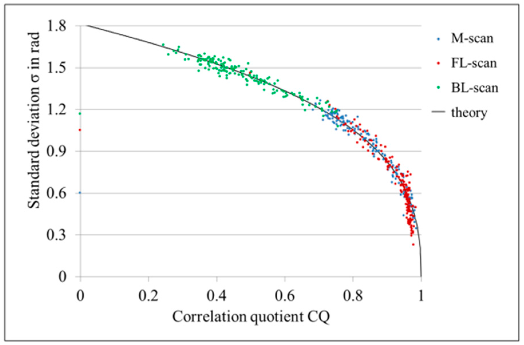
The correlation quotient CQ and the standard deviation σΔϕ against the radial position r inside the capillary in Figure 7b,c, show what can be visually expected from Figure 6c,d. For the M-scan (blue points), the backscattering signals of the Intralipid scatterers at the capillary border are highly correlated and show a small standard deviation of σΔϕ = 0.4 rad, in comparison to the capillary center with a reduced correlation of CQ = 0.73 and a phase shift noise of σΔϕ = 1.15 rad. For the forward lateral scan (red points), the correlation at the capillary center is strongly increased to CQ = 0.97 and the phase noise of the fast moving particles is highly reduced to σΔϕ = 0.4 rad compared to the M-scan. The experimentally measured CQ in Figure 7b shows that the maximum correlation of one is not achieved, possibly because of the Brownian motion of the Intralipid. However, it is evident that the velocity of the X-galvanometer scanner is matched very well to the oil particles for the FL-scan, since the behavior of the phase noise σΔϕ of the M-scan (blue points) and the FL-scan (red points) is inverted, as presented in Figure 7c. The result of the BL-scan (green points) shows a strongly damped correlation and a high noise of the Doppler shift σΔϕ over the entire capillary, as expected. The relation of σΔϕ and CQ are empirically determined in [20] and presented as a solid line in Figure 8 besides the very well fitting measurement values. Since the correlation quotient CQ is indirectly proportional to the Doppler noise σΔϕ, CQ provides no added value for the analysis of LR-DOCT, for which reason, only σΔϕ is presented for the following in vitro blood flow measurements.
4.2. LR-DOCT with In Vitro Blood Flow
In analogy to the Intralipid flow experiment, measurements are performed with the identical capillary model in combination with diluted fresh human blood. The measured Doppler angle ϑ amounts to 1.7°. Since the flow rate is set to 8 mL/h, the measurement parameters concerning the tracked transverse velocities are similar to the Intralipid flow phantom in Section 4.1. Exemplary structural images of the detected M-scans, FL-scans, and BL-scans are found in Figure 9a,d for two data sets, each consisting of 400 A-scans.
Obviously, the speckle pattern is different to the experiments with Intralipid flow, first due to the larger size of the highly scattering wheel-shaped erythrocytes with a diameter of Ø ≈ 7.5 µm and a thickness of d ≈ 2.0 µm in comparison to the small spherical oil particles of the Intralipid, with a mean diameter of Ø ≈ 100 nm relative to the size of the sample beam of w0 = 9.3 µm at the focal plane. Secondly, this pattern is due to the inhomogeneous distribution of the erythrocytes of the diluted blood sample within the capillary. Nevertheless, the dilution described in Section 3.1 is necessary for the tracking of erythrocytes at the capillary center, otherwise the erythrocytes are already too dense at r = 0.5R. Unfortunately, no backscattering signal is achieved at a larger depth, probably due to the orientation of the erythrocytes in this capillary zone and the resulting angular intensity modulation in the glass capillary cross section [28]. However, the velocity of the galvanometer scanner can be matched with the transverse flow velocity of the erythrocytes at the capillary center with the chosen dilution, as seen in the FL-scan of Figure 9a,d. The FL-scans of the measurements A and B differentiate, because the group of erythrocytes in experiment A is tracked over a shorter distance than the group in B. Therewith, the challenge of LR-DOCT for blood flow measurement becomes apparent, which implies the random catch of erythrocytes at the capillary center and the selected depths within the capillary, respectively. Because of the shear flow-dependent movement and orientation of the erythrocytes, the appearance of erythrocytes at the capillary center in blood samples with reduced hematocrit is small. Generally, for blood samples and especially for diluted blood, sedimentation of the erythrocytes occurs, where the flow velocity is small, as within the syringe and the tubing system connecting the glass capillary with the infusion pump [29]. Consequently, the erythrocytes build aggregates in the form of chain-like stacks [30]. With the falling distance of the connecting tube in front of the capillary entry, sedimentation and agglomeration within the capillary are avoided. The aggregates are dispersed, but erythrocytes are still grouped and randomly orientated at the capillary center in the presented FL-scan. Considering the images with an overlaid Doppler phase shift and standard deviation in Figure 9b,c,e,f, it becomes apparent that the Doppler noise is decreased for the resonantly scanned erythrocytes (FL-scan). On closer examination, the phase shift of the resonantly detected erythrocytes still shows an increased noise in dependence on the amount of erythrocytes flowing above, which is considered in the analysis presented below. The reason for this effect might be the optical inhomogeneity of human blood caused by the higher refractive index inside the erythrocytes. The incident light passing a group of erythrocytes is randomly delayed within the B-scan, which causes random phase fluctuations beneath this area, as in our case at the capillary center. Multiple scattering causing Doppler shadows might worsen the effect.
The mean Doppler phase shift and the corresponding standard deviation of the diluted human blood flow are quantified for both experiments, and the results are presented in Figure 10. As seen, both measurements offer similar characteristics, which show the reproducibility of LR-DOCT. Moreover, the calculated phase shift is slightly higher for the FL-scan than for the M-scan in the depth range of resonantly detected erythrocytes. Additionally, the standard deviation of the mean phase shift is reduced (asterisk in Figure 10b,d) at the radial position r near the center of the capillary. Since the erythrocytes are not completely resonantly detected over the detected 400 A-scans, Δϕ and σΔϕ include the phase information of parts with no significant backscattering signal, which unfortunately increases σΔϕ.
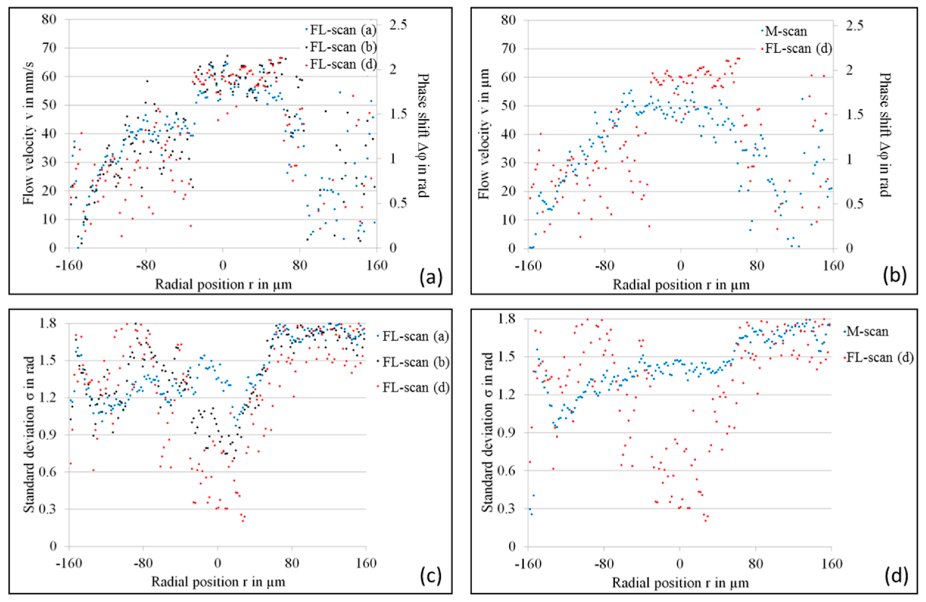
For a more precise analysis, parts of the trace with a high signal in the resonant region are selected, as shown in Figure 11. The number of lateral resonantly detected A-scans (originally N = 400 Figure 11a) is systematically reduced to N = 90 (Figure 11b), N = 40 (Figure 11c), and N = 22 (Figure 11d), showing an increased correlated backscattering signal at the capillary center with a decreasing number N of selected A-scans. Considering the diagram in Figure 12a, the Doppler phase shift of the resonantly detected erythrocytes at the capillary center differ slightly for N = 400 (Figure 11a), N = 90 (Figure 11b), and N = 22 (Figure 11d). Comparing Δϕ of the M-scan and the FL-scan with N = 22, one can identify a difference up to 0.4 rad and 10 mm/s, respectively, for the resonant detection (Figure 12b). The standard deviation of the mean phase shift is maximally reduced for N = 22 of the FL-scan and the resonantly scanned depths (cp. Figure 12c,d).
5. Summary and Conclusions
In the present study, lateral resonant Doppler optical coherence tomography (LR-DOCT) is proposed for velocity measurements of oblique sample motion with very small Doppler angles and high absolute sample velocities in spectral domain OCT (SD-OCT), where the nonlinear relation between the Doppler phase shift Δϕ and the axial velocity component vz hampers the accurate velocity calculation by the phase-resolved Doppler OCT (PR-DOCT). The described LR-DOCT overcomes the limitation of the nonlinear Δϕ-vz-relationship and allows the calculation of the axial sample velocity vz by matching the lateral scanner movement velocity with the transverse velocity component vx of the sample. LR-DOCT is validated by means of two flow phantoms with a 1% Intralipid emulsion and diluted human blood, respectively. The flow velocity at the capillary center is lateral resonantly detected by adapting the scanner velocity to the transverse velocity vx of the flowing scattering particles. By using an online display of the moving sample and accordingly the capillary flow before data acquisition, the transverse flow velocity vx can be estimated for the adjustment of the scanner velocity in LR-DOCT. Since the speckle pattern of highly correlated A-scans is clearly identifiable, the adaption of the lateral scanner velocity is simple. Due to the variable scan velocity of the galvanometer scanner, within its specifications, arbitrary flow velocities can be lateral resonantly measured by adapting the scanning protocol. Generally, LR-DOCT works very well for volume scatterers consisting of many small particles (e.g., 1% Intralipid flow) relative to the wavelength λ0 and the sample beam width w0 at the focal plane, whereas the method is limited for particles exceeding one or both of these factors (e.g., highly scattering erythrocytes of blood flow). The validation of the presented study has shown that LR-DOCT performs to a limited extent for diluted blood flow, where small groups of obliquely moving erythrocytes are resonantly detectable. This fact probably makes it difficult for in vivo blood flow measurements. Nevertheless, it is conceivable that LR-DOCT could produce precise blood flow measurements of easily accessible blood capillaries running almost perpendicular to the incident sample beam, containing only a few erythrocytes. Even though LR-DOCT has to be evaluated for in vivo conditions in future research, it is still interesting for many other moving samples in ex vivo and in vitro applications, or non-medical and non-biological configurations. Under the discussed conditions, LR-DOCT overcomes the nonlinear relation between the Doppler phase shift Δϕ and axial sample velocity, and with this, the limitation of PR-DOCT in SD-OCT for an oblique sample motion with a strong transverse velocity component. Consequently, LR-DOCT advantageously enables the simple, correct, and unlimited phase-resolved Doppler measurement of sample and flow velocities in SD-OCT.
Acknowledgments
We thank Peter Cimalla for the assistance with the dualband spectral domain OCT system and Christian Schnabel for the voluntary blood donation.
Author Contributions
All authors contributed to this work. Authors Julia Walther and Edmund Koch jointly developed the idea of LR-DOCT, performed the in vitro experiments, processed the acquired data, and analyzed the calculated Doppler information for the validation of LR-DOCT; Julia Walther wrote the paper.
Conflicts of Interest
The authors declare no conflict of interest.
References
- Huang, D.; Swanson, E.A.; Lin, C.P.; Schuman, J.S.; Stinson, W.G.; Chang, W.; Hee, M.R.; Flotte, T.; Gregory, K.; Puliafito, C.A.; et al. Optical Coherence Tomography. Science 1991, 254, 1178–1181. [Google Scholar] [CrossRef] [PubMed]
- Leitgeb, R.; Hitzenberger, C.; Fercher, A. Performance of Fourier domain vs. time domain optical coherence tomography. Opt. Express 2003, 11, 889–894. [Google Scholar] [CrossRef] [PubMed]
- Choma, M.; Sarunic, M.; Yang, C.; Izatt, J. Sensitivity advantage of swept source and Fourier domain optical coherence tomography. Opt. Express 2003, 11, 2183–2189. [Google Scholar] [CrossRef] [PubMed]
- De Boer, J.F.; Cense, B.; Park, B.H.; Pierce, M.C.; Tearney, G.J.; Bouma, B.E. Improved signal-to-noise ratio in spectral-domain compared with time-domain optical coherence tomography. Opt. Lett. 2003, 28, 2067–2069. [Google Scholar] [CrossRef] [PubMed]
- Huber, R.; Wojtkowski, M.; Fujimoto, J.G. Fourier domain mode locking (FDML): A new laser operating regime and applications for optical coherence tomography. Opt. Express 2006, 14, 3225–3237. [Google Scholar] [CrossRef] [PubMed]
- Kirsten, L.; Domaschke, T.; Schneider, C.; Walther, J.; Meissner, S.; Hampel, R.; Koch, E. Visualization of dynamic boiling processes using high-speed optical coherence tomography. Exp. Fluids 2015, 56. [Google Scholar] [CrossRef]
- Hitzenberger, C.K.; Gützinger, E.; Sticker, M.; Pircher, M.; Fercher, A.F. Measurement and imaging of birefringence and optic axis orientation by phase resolved polarization sensitive optical coherence tomography. Opt. Express 2001, 9, 780–790. [Google Scholar] [CrossRef] [PubMed]
- Pircher, M.; Hitzenberger, C.K.; Schmidt-Erfurth, U. Polarization sensitive optical coherence tomography in the human eye. Prog. Retin. Eye Res. 2011, 30, 431–451. [Google Scholar] [CrossRef] [PubMed]
- Faber, D.J.; Mik, E.G.; Aalders, M.C.G.; van Leeuwen, T.G. Toward assessments of blood oxygen saturation by spectroscopic optical coherence tomography. Opt. Lett. 2005, 30, 1015–1017. [Google Scholar] [CrossRef] [PubMed]
- Srinivasan, V.J.; Sakadzić, S.; Gorczynska, I.; Ruvinskaya, S.; Wu, W.C.; Fujimoto, J.G.; Boas, D.A. Quantitative cerebral blood flow with optical coherence tomography. Opt. Express 2010, 18, 2477–2494. [Google Scholar] [CrossRef] [PubMed]
- Leitgeb, R.A.; Werkmeister, R.M.; Blatter, C.; Schmetterer, L. Doppler optical coherence tomography. Prog. Retin. Eye Res. 2014, 41, 26–43. [Google Scholar] [CrossRef] [PubMed]
- Zhao, Y.H.; Chen, Z.P.; Saxer, C.; Xiang, S.H.; de Boer, J.F.; Nelson, J.S. Phase-resolved optical coherence tomography and optical Doppler tomography for imaging blood flow in human skin with fast scanning speed and high velocity sensitivity. Opt. Lett. 2000, 25, 114–116. [Google Scholar] [CrossRef] [PubMed]
- Leitgeb, R.; Schmetterer, L.; Drexler, W.; Fercher, A.; Zawadzki, R.; Bajraszewski, T. Real-time assessment of retinal blood flow with ultrafast acquisition by color Doppler Fourier domain optical coherence tomography. Opt. Express 2003, 11, 3116–3121. [Google Scholar] [CrossRef] [PubMed]
- Vakoc, B.; Yun, S.; de Boer, J.; Tearney, G.; Bouma, B. Phase-resolved optical frequency domain imaging. Opt. Express 2005, 13, 5483–5493. [Google Scholar] [CrossRef] [PubMed]
- Grulkowski, I.; Gorczynska, I.; Szkulmowski, M.; Szlag, D.; Szkulmowska, A.; Leitgeb, R.; Kowalczyk, A.; Wojtkowski, M. Scanning protocols dedicated to smart velocity ranging in spectral OCT. Opt. Express 2009, 17, 23736–23754. [Google Scholar] [CrossRef] [PubMed]
- Walther, J.; Koch, E. Relation of joint spectral and time domain optical coherence tomography (jSTdOCT) and phase-resolved Doppler OCT. Opt. Express 2014, 22, 23129–23146. [Google Scholar] [CrossRef] [PubMed]
- Bachmann, A.H.; Villiger, M.L.; Blatter, C.; Lasser, T.; Leitgeb, R.A. Resonant Doppler flow imaging and optical vivisection of retinal blood vessels. Opt. Express 2007, 15, 408–422. [Google Scholar] [CrossRef] [PubMed]
- Koch, E.; Hammer, D.; Wang, S.; Cuevas, M.; Walther, J. Resonant Doppler imaging with common path OCT. Proc. SPIE 2009, 7372, 737220. [Google Scholar]
- Koch, E.; Walther, J.; Cuevas, M. Limits of Fourier domain Doppler-OCT at high velocities. Sens. Actuators A 2009, 156, 8–13. [Google Scholar] [CrossRef]
- Walther, J.; Koch, E. Transverse motion as a source of noise and reduced correlation of the Doppler phase shift in spectral domain OCT. Opt. Express 2009, 17, 19698–19713. [Google Scholar] [CrossRef] [PubMed]
- Walther, J.; Koch, E. Impact of a detector dead time in phase resolved Doppler analysis using spectral domain optical coherence tomography. J. Opt. Soc. Am. A 2017, 34, 241–251. [Google Scholar] [CrossRef] [PubMed]
- Wehbe, H.; Ruggeri, M.; Jiao, S.; Gregori, G.; Puliafito, C.A.; Zhao, W. Automatic retinal blood flow calculation using spectral domain optical coherence tomography. Opt. Express 2007, 15, 15193–15206. [Google Scholar] [CrossRef] [PubMed]
- Cimalla, P.; Walther, J.; Mehner, M.; Cuevas, M.; Koch, E. Simultaneous dual-band optical coherence tomography in the spectral domain for high resolution in vivo imaging. Opt. Express 2009, 17, 19486–19500. [Google Scholar] [CrossRef] [PubMed]
- Walther, J.; Mueller, G.; Meissner, S.; Cimalla, P.; Homann, H.; Morawietz, H.; Koch, E. Time-resolved blood flow measurement in the in vivo mouse model by optical frequency domain imaging. Proc. SPIE 2009, 7372, 73720J. [Google Scholar]
- Walther, J.; Mueller, G.; Morawietz, H.; Koch, E. Analysis of in vitro and in vivo bidirectional flow velocities by phase-resolved Doppler Fourier-domain OCT. Sens. Actuators A 2009, 156, 14–21. [Google Scholar] [CrossRef]
- Langbein, H.; Brunssen, C.; Hoffmann, A.; Cimalla, P.; Brux, M.; Bornstein, S.R.; Deussen, A.; Koch, E.; Morawietz, H. NADPH oxidase 4 protects against development of endothelial dysfunction and atherosclerosis in LDL receptor deficient mice. Eur. Heart J. 2016, 37, 1753–1761. [Google Scholar] [CrossRef] [PubMed]
- Vakoc, B.J.; Tearney, G.J.; Bouma, B.E. Statistical properties of phase-decorrelation in phase-resolved Doppler optical coherence tomography. IEEE Trans. Med. Imaging 2009, 28, 814–821. [Google Scholar] [CrossRef] [PubMed]
- Cimalla, P.; Walther, J.; Mittasch, M.; Koch, E. Shear flow-induced optical inhomogeneity of blood assessed in vivo and in vitro by spectral domain optical coherence tomography in the 1.3 µm wavelength range. J. Biomed. Opt. 2011, 16, 116020. [Google Scholar] [CrossRef] [PubMed]
- Douglas-Hamilton, D.H.; Smith, N.G.; Kuster, C.E.; Vermeiden, J.P.W.; Althouse, G.C. Particle distribution in low-volume capillary-loaded chambers. J. Androl. 2005, 26, 107–114. [Google Scholar] [PubMed]
- Friebel, M.; Helfmann, J.; Müller, G.; Meinke, M. Influence of shear rate on the optical properties of human blood in the spectral range 250 to 1100 nm. J. Biomed. Opt. 2007, 12, 054005. [Google Scholar] [CrossRef] [PubMed]
Figure 1.
Contour plots of the numerically calculated phase shift Δϕ between consecutive A-scans as a function of the normalized transverse δx and axial δz displacement of the oblique sample motion [20,21] for detector dead times ΔT/TA-scan of (a) 0.0 and (b) 0.05. The central dashed line with ϑ′ of 29° corresponds to the expected phase shift of the 1% Intralipid flow experiment presented in Section 4. Additional shifted dashed lines with ϑ′ of 29° are given for the LR-scanning explained in Section 2.2.

Figure 2.
Schematic of the obliquely moving scattering sample relative to (a) a static Gaussian sample beam, (b) a forward lateral, and (c) a backward lateral scanning beam. (a) Due to the limited width of the incident Gaussian sample beam and the transverse motion component, the detected axial displacement Δz is reduced to Δzd. (b) If the lateral scanning speed is matched with the transverse velocity of the obliquely moving scatterers, the sample movement is detected as purely axial displacement during TA-scan. (c) If the sample beam scanning is opposite to the sample movement, the phase correlation is strongly reduced, for which Δz is measured significantly lower.
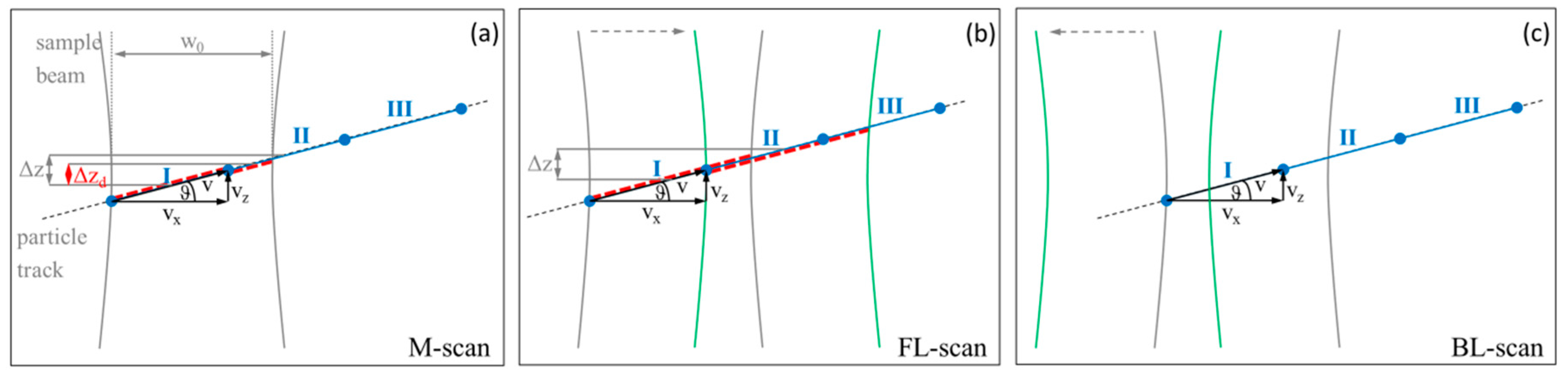
Figure 3.
Dualband SD-OCT system, where the long wavelength band centered at 1250 nm with a full spectral width of 200 nm is used with a fiber-coupled customized scanning unit. Abbreviations: SMF: single mode fiber, C: collimator, BS: beam splitter, DC: dichroic mirror, ϑ: Doppler angle. The flow phantom consists of a 312 µm glass capillary connected to an infusion pump by a tubing system and filled with 1% Intralipid and diluted fresh human blood, respectively.
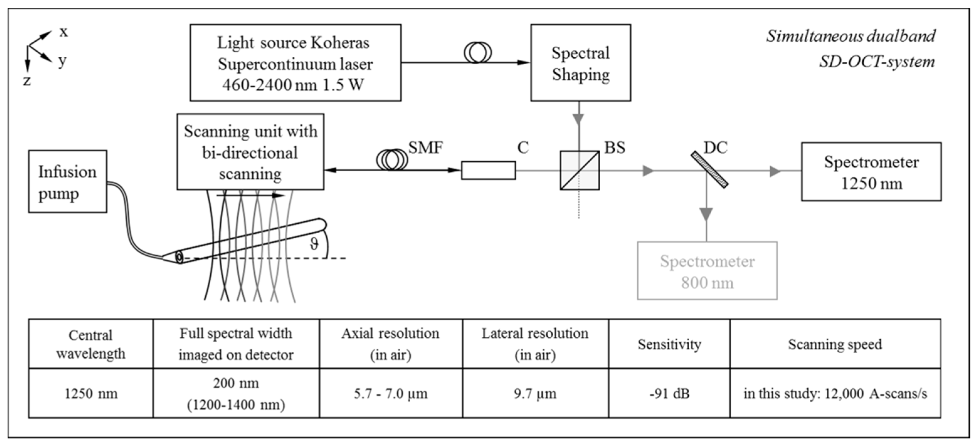
Figure 4.
Conventional (a) and bi-directional lateral (d) scanning protocol of the X- and Y-galvanometer scanners. (b) Cross section and longitudinal section of the Intralipid-filled glass capillary generated from the detected 3D-scan. (c) Schematic of the imaged glass capillary in respect to the defined coordinate system. (e) Resulting M-scan and B-scans (forward and backward lateral scan: FL- and BL-scan) due to the modified scanning protocol for LR-DOCT.
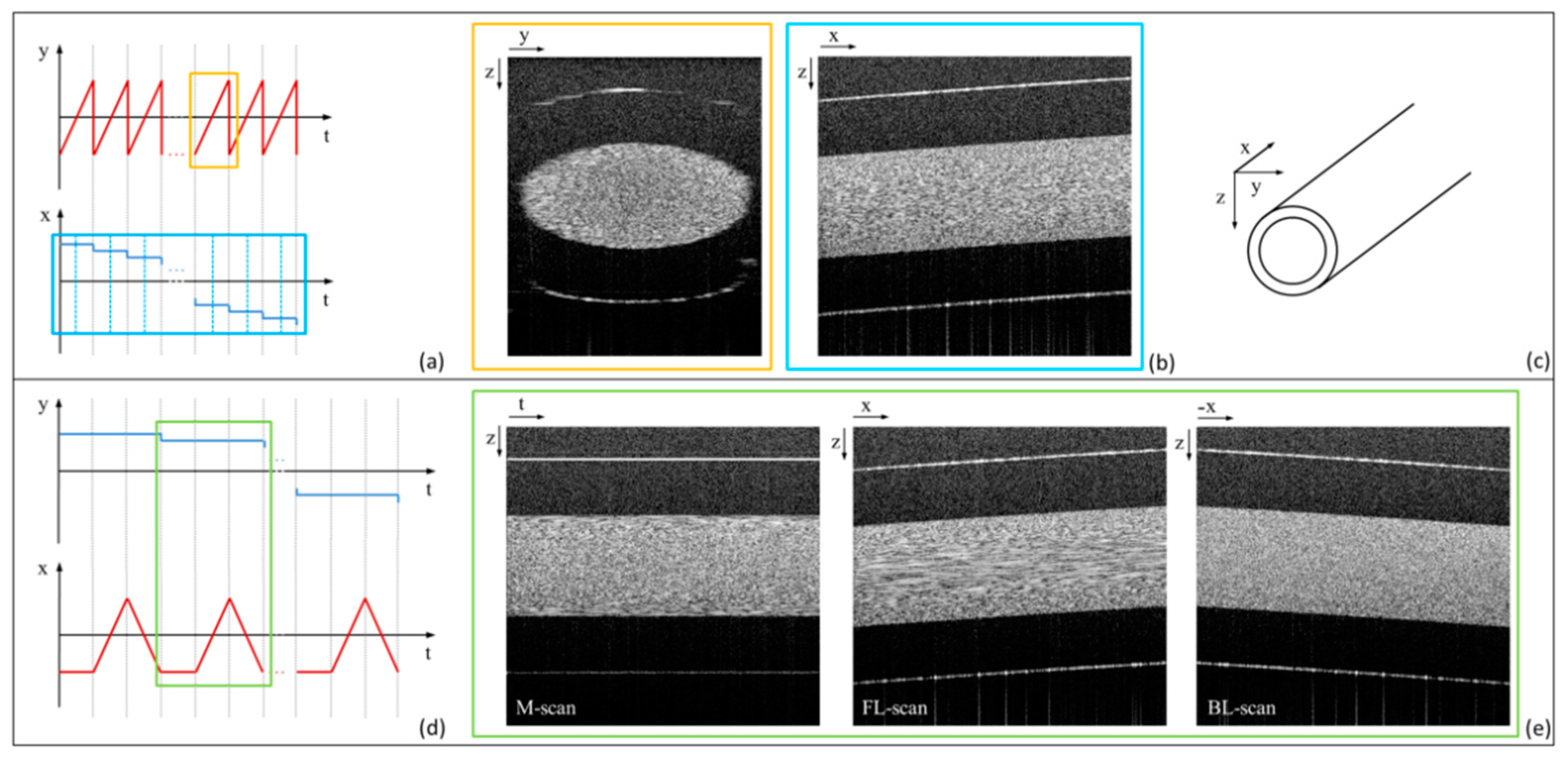
Figure 5.
(a) Conventional processing of the detected interferometric signals for structural and Doppler flow imaging on the example of the FL-scan of the 1% Intralipid flow within the glass capillary. (b) Correction of the obliquely running direction of the glass capillary by insertion of an additional phase term ϕshifted(k,j) to the real-valued interference signal and subsequent conventional processing. Note the tilted signal from zero delay at the top.

Figure 6.
(a) Grayscale structural SD-OCT images of the M-scan, the forward (FL-scan) and backward lateral Doppler scan (BL-scan) of the 1% Intralipid flow through a 312 µm glass capillary. (b) Corresponding phase-resolved Doppler flow images for the measured Doppler angle ϑ of 1.7°. (c) Colored correlation images representing the correlation quotient CQ in accordance to [20,21]. (d) Standard deviation σΔϕ of the mean Doppler phase shift of 512 single A-scans overlaid to the structural images.

Figure 7.
(a) Calculated and fitted flow profiles of the flowing 1% Intralipid as a function of the radial position r inside the 312 µm capillary for the M-scan (blue points), the forward (FL-scan, red points) and backward lateral scan (BL-scan, green points). Additionally, the correlation quotient CQ (b) and the standard deviation σΔϕ (c) are shown versus r for the detected M-scan, the FL-scan and the BL-scan.

Figure 8.
Mean error (standard deviation) σΔϕ is shown theoretically (solid line [20]) and experimentally (measurement points of the M-scan, FL-scan, and BL-scan) as a function of CQ.
Figure 8.
Mean error (standard deviation) σΔϕ is shown theoretically (solid line [20]) and experimentally (measurement points of the M-scan, FL-scan, and BL-scan) as a function of CQ.

Figure 9.
Grayscale structural images (a,d) and phase-resolved Doppler images (b,e) are shown of the M-scans, FL-scans, and BL-scans each consisting of 400 A-scans for two experiments A and B with identical settings. In addition, the standard deviation of the mean Doppler phase shift of 400 A-scans is overlaid to the structural image for both experiments (c,f).
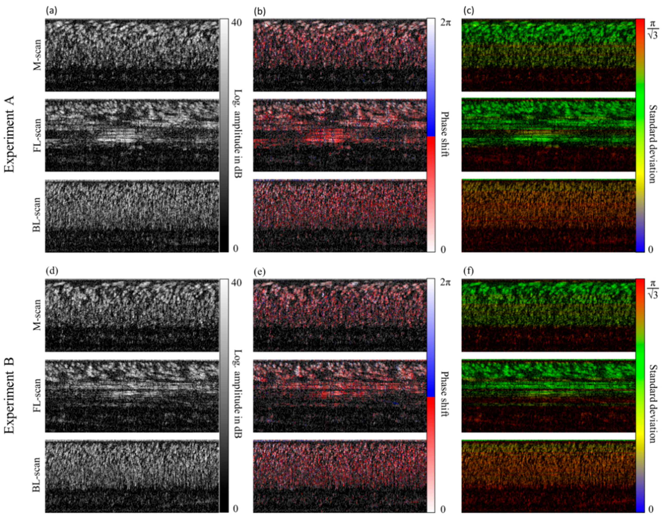
Figure 10.
(a,c) Calculated mean Doppler phase shift Δϕ and resulting flow profile of the diluted blood flow of experiment A and B are presented as a function of the radial position r for the detected M-scan, FL-scan and BL-scan. (b,d) Corresponding standard deviation σΔϕ of the mean phase shift versus the radial position r of the capillary lumen. The asterisk marks the radial position with strongly reduced σΔϕ obtained with the FL-scan near the center of the capillary.
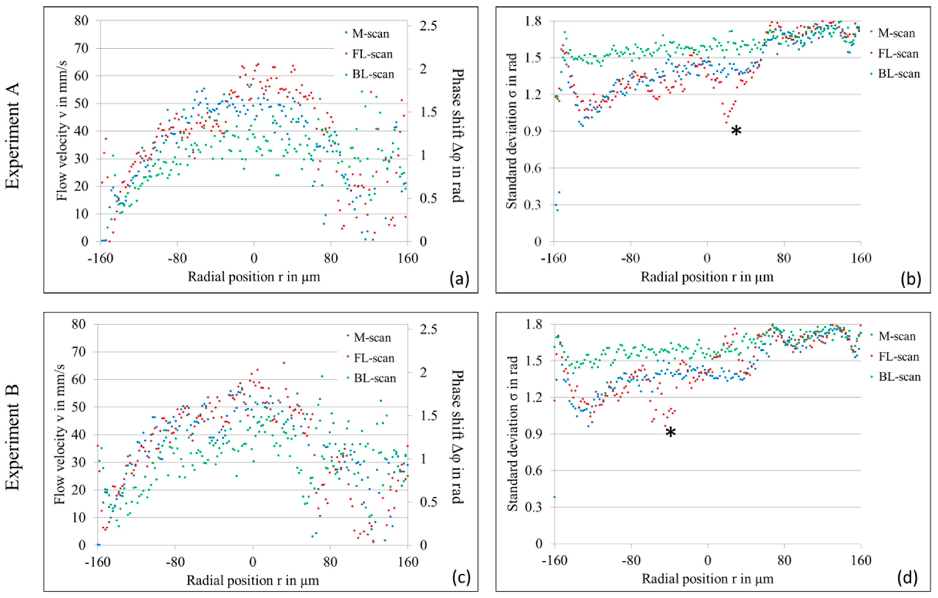
Figure 11.
Structural, Doppler flow, and Doppler noise images of the forward lateral scan (FL-scan) of the diluted blood flow through the 312 µm glass capillary are presented for N = 400 (a), N = 90 (b), N = 40 (c), and N = 22 (d) analyzed A-scans.
Figure 11.
Structural, Doppler flow, and Doppler noise images of the forward lateral scan (FL-scan) of the diluted blood flow through the 312 µm glass capillary are presented for N = 400 (a), N = 90 (b), N = 40 (c), and N = 22 (d) analyzed A-scans.

Figure 12.
(a) Calculated Doppler phase shift of the FL-scans in Figure 11a,b,d are shown as a function of the radial position r. (b) Doppler phase shift of the FL-scan in Figure 11d in comparison to the phase shift of the M-scan in Figure 9b. (c,d) Corresponding standard deviation of the mean Doppler phase shift presented in (a,b).
© 2017 by the authors. Licensee MDPI, Basel, Switzerland. This article is an open access article distributed under the terms and conditions of the Creative Commons Attribution (CC BY) license (http://creativecommons.org/licenses/by/4.0/).
Share and Cite
MDPI and ACS Style
Walther, J.; Koch, E. Flow Measurement by Lateral Resonant Doppler Optical Coherence Tomography in the Spectral Domain. Appl. Sci. 2017, 7, 382. https://doi.org/10.3390/app7040382
AMA Style
Walther J, Koch E. Flow Measurement by Lateral Resonant Doppler Optical Coherence Tomography in the Spectral Domain. Applied Sciences. 2017; 7(4):382. https://doi.org/10.3390/app7040382
Chicago/Turabian StyleWalther, Julia, and Edmund Koch. 2017. "Flow Measurement by Lateral Resonant Doppler Optical Coherence Tomography in the Spectral Domain" Applied Sciences 7, no. 4: 382. https://doi.org/10.3390/app7040382
Note that from the first issue of 2016, this journal uses article numbers instead of page numbers. See further details here.