Improved Tensor-Based Singular Spectrum Analysis Based on Single Channel Blind Source Separation Algorithm and Its Application to Fault Diagnosis

Abstract

To solve the problem of multi-fault blind source separation (BSS) in the case that the observed signals are under-determined, a novel approach for single channel blind source separation (SCBSS) based on the improved tensor-based singular spectrum analysis (TSSA) is proposed. As the most natural representation of high-dimensional data, tensor can preserve the intrinsic structure of the data to the maximum extent. Thus, TSSA method can be employed to extract the multi-fault features from the measured single-channel vibration signal. However, SCBSS based on TSSA still has some limitations, mainly including unsatisfactory convergence of TSSA in many cases and the number of source signals is hard to accurately estimate. Therefore, the improved TSSA algorithm based on canonical decomposition and parallel factors (CANDECOMP/PARAFAC) weighted optimization, namely CP-WOPT, is proposed in this paper. CP-WOPT algorithm is applied to process the factor matrix using a first-order optimization approach instead of the original least square method in TSSA, so as to improve the convergence of this algorithm. In order to accurately estimate the number of the source signals in BSS, EMD-SVD-BIC (empirical mode decomposition—singular value decomposition—Bayesian information criterion) method, instead of the SVD in the conventional TSSA, is introduced. To validate the proposed method, we applied it to the analysis of the numerical simulation signal and the multi-fault rolling bearing signals.

1. Introduction

In the field of mechanical fault diagnosis, vibration signals always contain a wealth of information about equipment operating status. Thus, a powerful signal processing method is necessary to extract the possible faults [1,2,3,4]. Generally, various sensors are used to obtain the vibration signals of the mechanical equipment. Characteristic information, such as fault feature frequencies, can be extracted from the obtained vibration signals [5,6]. However, one mechanical fault is usually accompanied by other faults. For example, simultaneous gear fault and bearing fault are common in a damaged decelerator. Therefore, the acquired signal is generally coupled by multiple fault signals along with the background noise, which brings out a consequence that the characteristics of the fault component cannot be directly identified. As an effective approach to solve the problem of complex multiple faults, blind source separation (BSS) can be used to separate the linear mixtures of different unknown source signals [7,8,9,10]. Since the limitation by the cost of equipment, installation conditions and others cases, the measurement scheme using a single sensor is generally considered. Consequently, we can only obtain single channel complex multiple faults signals. Therefore, the research on the fault diagnosis method of rotating machinery under single channel condition has a very wide range of engineering applications.

The single channel blind source separation (SCBSS) [11], which can separate each source signal from the collected composite signals obtained by single sensor, is a special case in BSS. However, compared with BSS, there is a serious problem that the number of source signals is not less than the number of observation signals in SCBSS. Hence, the signal decomposition is needed to achieve the SCBSS. In the study of complex fault diagnosis under single channel condition, the general solution to this problem is not unique and various approaches have been proposed, ranging from applying independence assumptions to non-negativity and sparsity constraints [12]. Currently, research in this area mainly focuses on the virtual multi-channel method. The space-time method was first proposed by Davies and James [13]. After obtaining a virtual multi-channel signals by delaying the single mixed observation signal, the independent component analysis (ICA) [14] algorithm was utilized to separate the source signals from the obtained virtual multi-channel signals. Hong [15] applied wavelet decomposition to the single-channel signal and a virtual multi-channel signals using sub-frequency band signals was obtained, followed by employing the ICA method. Mijovic et al. [16] proposed the Ensemble Empirical Mode Decomposition (EEMD) [17] to decompose the mixed single channel signal into a plurality of intrinsic mode functions (IMF_S). Moreover, Wang et al. [18] proposed a new method to achieve the separation of complex fault signals by combining with the EEMD and the ICA method. Guo et al. [19] also discovered that the EEMD-ICA method can reduce the dimension to solve the single channel separation problem. Wu et al. [20] applied the EMD-ICA method to the simulation research of bearings and gears with mixed faults. The common character of SCBSS method is based on a virtual multi-channel signal, which is constructed as the input data of the separation algorithm, thus we can obtain a better separation effect. However, the constructed multi-channel signal by the above-mentioned method is difficult to maintain the characteristics of the observed signal, and it may be interfered by the noise or other components. Hence, the frequency domain characteristics of separated signals may be distorted, and a good separation effect may not be achieved. The above methods mainly use EMD or the improved EMD to construct virtual multi-channel signals, which can transform underdetermined condition to positive definite condition in BSS. However, EMD still have some problems, such as modal aliasing [21] and edge effect [22]. Therefore, the traditional SCBSS method has obvious deficiencies in the analysis of multi-faults.

Compared with a one-dimensional space, a multi-dimensional signal always contains more information. As the most natural representation of multi-dimensional data, tensor can preserve the intrinsic structure of the data to the maximum extent. Tensor decomposition method can extract the useful components in the original measured vibration signal. Consequently, the tensor decomposition algorithm has broad application prospects in signal processing and has great practical engineering significance in some aspects such as pattern recognition and big data processing. CANDECOMP/PARAFAC (CP) decomposition [23,24] is a commonly used tensor decomposition method. If the rank of the tensor is R, the CP decomposition can factorize a tensor into a sum of R-component rank-one tensors [25]. By the proposed decomposition model, three factor matrixes representing the combination of the vectors can be obtained from the rank-one components. Recently, the tensor-based singular spectrum analysis (TSSA) algorithm, which provides an effective way for solving the above problem of SCBSS, was proposed by Saeid et al. [26] and has been applied to the field of EEG signal processing. Firstly, the one-dimensional times series can be segmented as a matrix using a non-overlapping window. Then, each row of matrix can be expressed as a reconstructed attractor matrix through phase space reconstruction [27]. The obtained every reconstructed attractor matrix formed the corresponding slice of the tensor, thus a 3D tensor was obtained to be decomposed. Then, the above-mentioned CP tensor decomposition method was used here. The key step is performed by the alternating least squares method (ALS) [28] to obtain the three-factor matrix. The TSSA method combines the advantages of the phase space reconstruction, the SSA [29], and the tensor decomposition. However, the TSSA still has some problems when applied to the SCBSS, mainly including unsatisfactory convergence and poor estimating accuracy of the number of the original signals.

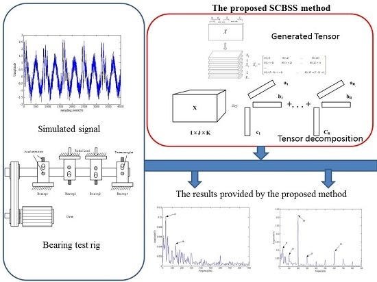
In this paper, an improved TSSA decomposition method using the weighted optimization CP tensor decomposition model is proposed. The improve method is the so-called CANDECOMP/PARAFAC weighted optimization (CP-WOPT), which is defined as the first-order optimization to solve the least squares objective function over all the factor matrices simultaneously, so as to improve the convergence of this algorithm. Faced with the difficulty in determining the number of original signals, a commonly accepted method is introduced, namely EMD-SVD-BIC [30], which can estimate the number of original signals accurately. Firstly, the intrinsic mode functions (IMF_S) of a signal are obtained by using the EMD method. Then, the singular value decomposition (SVD) on the matrix is performed, which consists of the IMF_S from the observed signal using SVD. We can obtain the distribution of eigenvalues about the source data. Finally, the BIC is used here to judge the number of source signals. The validity of the proposed method is verified by the numerical simulation signal and the measured vibration signal of the fault test bench in public dataset.

The rest of this paper is structured as follows: In Section 2, the basic theory introductions of the TSSA algorithm and blind source separation are briefly described. Then, the proposed single channel blind source separation (SCBSS) method based on the CP-WOPT model is developed. The analysis results of numerical simulation signal and bearing fault signal are, respectively, described in Section 3 and Section 4. Section 5 concludes the paper.

2. Theory

2.1. The TSSA Algorithm

The TSSA method mainly contains two stages, the embedding operation process and the tensor decomposition process. In the embedding stage, a one-dimensional time series $\mathit{x}$ with length n is mapped into a 3D tensor $\mathcal{X}$.

In the embedding stage, two works need to be achieved. Firstly, $\mathit{x}$ is segmented as a matrix $\mathit{X}$ with the size of $[n/l]\times l$ by using a non-overlapping window of size $l$, and the obtained matrix $\mathit{X}$ is shown as:

$$\mathit{X}=\left(\begin{array}{llll}\mathit{x}(1)& \mathit{x}(2)& \dots & \mathit{x}(l)\\ \mathit{x}(l+1)& \mathit{x}(l+2)& \dots & \mathit{x}(2l)\\ \dots \\ \mathit{x}(I-1)*l& \mathit{x}(I-1)*l+1& \dots & \mathit{x}n\end{array}\right)$$

(1)

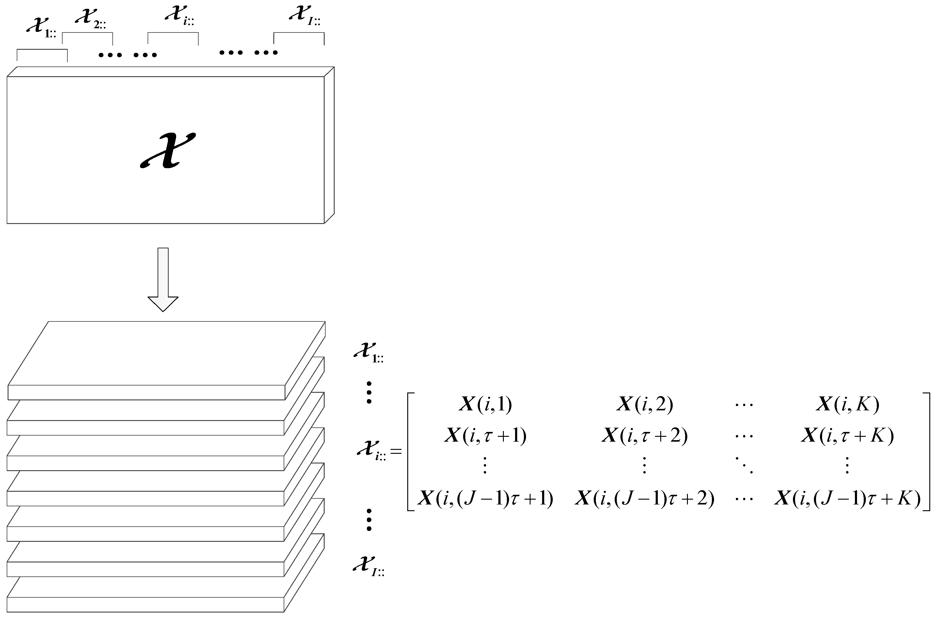
Then, the matrix $\mathit{X}$ is converted to tensor $\mathcal{X}$, as demonstrated in Figure 1. Each slice of the $\mathcal{X}$ is a reconstructed attractor matrix, which comes from the row of matrix $\mathit{X}$ through phase space reconstruction. The segmentation is performed in one direction.

The slice ${\mathcal{X}}_{i::}$ of tensor $\mathcal{X}$ in Figure 1 is formed from the $i$-th row of matrix $\mathit{X}$ using the phase space reconstruction. In Figure 1, $K$ is the reconstructed window length, $J$ is the reconstructed embedding dimension and $\mathsf{\tau }$ is the delay time. Moreover, we know that $l=(J-1)\times \mathsf{\tau }+K$. The way of converting a matrix to a tensor can be explained by the following Equation:

$${\mathcal{X}}_{ijk}=\mathit{X}(i,(k+(j-1)\times \mathsf{\tau })),i=1,2,\dots ,I;j=1,2,\dots ,J;k=1,2,\dots ,K$$

(2)

where $J$ and $\mathsf{\tau }$ can be determined by the False Nearest Neighbor algorithm (FNN) [31], thus we can obtain a 3D tensor with the size $I\times J\times K$.

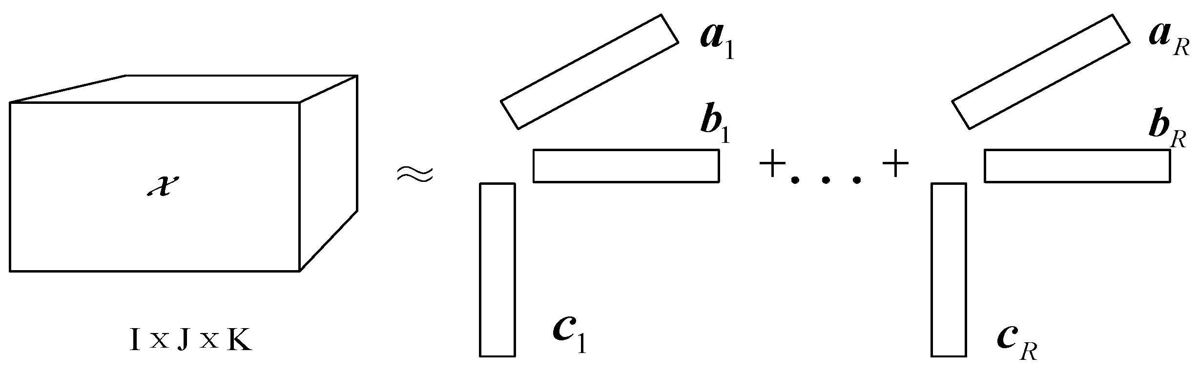
In the second stage, the obtained 3D tensor needs to be decomposed. The CP tensor decomposition method, which factorizes a tensor into a sum of component rank-one tensors, is used here. It can be considered as a generalization of bilinear principal component analysis (PCA) [32,33]. The fundamental expression of the CP based on outer product of the three factor matrices is given as [34,35]:

$$\mathcal{X}={\displaystyle \sum _{r=1}^R{\mathit{a}}_r\circ {\mathit{b}}_r\circ {\mathit{c}}_r}+\mathit{ℰ}$$

(3)

where $R$ is the rank of tensor $\mathcal{X}$. ${\mathit{a}}_r\in R^{I\times 1}$, ${\mathit{b}}_r\in R^{J\times 1}$ and ${\mathit{c}}_r\in R^{K\times 1}$ are the vector elements of factor matrices $\mathit{A}\in R^{I\times R}$, $\mathit{B}\in R^{J\times R}$, $\mathit{C}\in R^{K\times R}$. Tensor $ℰ\in R^{I\times J\times K}$ is the residual term. Hence, the CP model can be approximately expressed as:

$$\mathcal{X}\approx 〚\mathit{A},\mathit{B},\mathit{C}〛={\displaystyle \sum _{r=1}^R{\mathit{a}}_r\circ {\mathit{b}}_r\circ {\mathit{c}}_r}$$

(4)

The above-mentioned decomposition model is shown in Figure 2.

The TSSA algorithm uses the iterative least squares method to seek the factor matrix, namely CP-ALS, and the main ideal of the algorithm is to make the following error function to reach a minimum:

$$f(\mathit{A},\mathit{B},\mathit{C})=\frac{1}{2}{\Vert \mathcal{X}-〚\mathit{A},\mathit{B},\mathit{C}〛\Vert }^2$$

(5)

First, $\mathit{A}$, $\mathit{B}$, and $\mathit{C}$ should be given an initial matrix which is generally the random factor matrix. Then, $\mathit{B}$ and $\mathit{C}$ are fixed to solve for $\mathit{A}$; $\mathit{A}$ and $\mathit{C}$ are fixed to solve for $\mathit{B}$; and $\mathit{A}$ and $\mathit{B}$ are fixed to solve for $\mathit{C}$ in an alternating fashion until reaching some convergence. However, the convergence of tensor decomposition may be poor using the iterative least squares method, which will lead to an unstable or even wrong result. Thus, we develop an improved TSSA algorithm based on the CP-WOPT model in this paper.

2.2. The Improved TSSA Algorithm Based on CP-WOPT Model

Due to the poor decomposition convergence of the CP-ALS algorithm, the CANDECOMP/PARAFAC weighted optimization (CP-WOPT) approach is employed as the optimization algorithm. A non-negative weights tensor $\mathcal{W}\in R^{I\times J\times K}$ with the same size as $\mathcal{X}$ is defined. If most of the entries in $\mathcal{X}$ are zero or $\mathcal{X}$ is a sparse tensors, the tensor $\mathcal{W}$ will be a zero tensor as ${\mathcal{W}}_{i_1{i}_2\dots i_N}=0$. Otherwise, the element of tensor $\mathcal{W}$ is equal to 1 as ${\mathcal{W}}_{i_1{i}_2\dots i_N}=1$. Equation (5) can be replaced by:

$$f_{\mathcal{W}}(\mathit{A},\mathit{B},\mathit{C})=\frac{1}{2}{\Vert \mathcal{W}*\mathcal{X}-〚\mathit{A},\mathit{B},\mathit{C}〛\Vert }^2$$

(6)

Let $\mathcal{Y}=\mathcal{W}*\mathcal{X}$, $\mathcal{Z}=\mathcal{W}*〚\mathit{A},\mathit{B},\mathit{C}〛$. The tensor $\mathcal{Y}$ can be fixed as neither $\mathcal{W}$ nor $\mathcal{X}$ change during the iterations, and tensor $\mathcal{Z}$ represents the weighted reconstruction tensor of CP decomposition. Thus, Equation (6) is equivalent to:

$$f_{\mathcal{W}}(\mathit{A},\mathit{B},\mathit{C})=\frac{1}{2}{\Vert \mathcal{Y}-\mathcal{Z}\Vert }^2$$

(7)

The goal of CP-WOPT algorithm is to obtain the factor matrix$\mathit{A}$, $\mathit{B}$, $\mathit{C}$ to minimize the weighted error function defined in Equation (6). The algorithm based on the gradient method, which has better convergence performance, is used to solve Equation (7). Let ${\mathit{A}}^{-1}=\mathit{B}\odot \mathit{C}$, ${\mathit{B}}^{-1}=\mathit{A}\odot \mathit{C}$, and ${\mathit{C}}^{-1}=\mathit{A}\odot \mathit{B}$, where the operator $\odot$ denotes Khatri–Rao product of two matrices. Then, the gradient values is defined as follows [36]:

$$\frac{\partial f_{\mathcal{W}}}{\partial \mathit{A}}=({\mathcal{Z}}_{(1)}-{\mathcal{Y}}_{(1)}){\mathit{A}}^{-1}$$

(8)

$$\frac{\partial f_{\mathcal{W}}}{\partial \mathit{B}}=({\mathcal{Z}}_{(2)}-{\mathcal{Y}}_{(2)}){\mathit{B}}^{-1}$$

(9)

$$\frac{\partial f_{\mathcal{W}}}{\partial \mathit{C}}=({\mathcal{Z}}_{(3)}-{\mathcal{Y}}_{(3)}){\mathit{C}}^{-1}$$

(10)

Consequently, we can find the minimum value of the error function based on gradient values to estimate the value of each factor matrix.

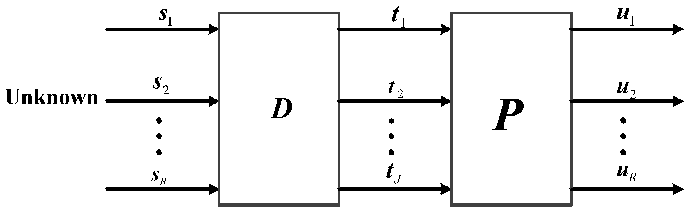
2.3. The Basic Theory of Blind Source Separation

Assume that there are $R$ source signals being linearly mixed into $J$ observed signals. For each signal, N samples are available. The following BSS model is considered:

$$\mathit{T}=\mathit{D}\mathit{S}+\mathit{N}$$

(11)

where $\mathit{T}=[{\mathit{t}}_1,{\mathit{t}}_2,\dots ,{\mathit{t}}_J]\in R^{N\times J}$ contains the observed data, $\mathit{S}=[{\mathit{s}}_1,{\mathit{s}}_2,\dots ,{\mathit{s}}_R]\in R^{N\times R}$ with the R unknown source signals. $\mathit{D}\in R^{R\times J}$ represents the unknown composite matrix and $\mathit{N}\in R^{N\times J}$ denotes additive noise. Commonly, the problem of BSS can be divided into three situations: the underdetermined BSS with the condition of $R>J$; the positive definite BSS if $R=J$; and the over-determined BSS when $R<J$. A clearly model of BSS is as shown as Figure 3.

The general goal in BSS is to recover the unknown source in $\mathit{S}$ and the unknown composite vectors in $\mathit{D}$, given only the observed data $\mathit{T}$, as shown in Figure 3. The research of this paper is concerned about the single channel underdetermined BSS, namely SCBSS, which means the number of observed signals is less than that of the source signals and the number $J$ is equal to 1. Hence, the observed data $\mathit{T}$ will be a vector with length n. Therefore, the target of SCBSS is to obtain the unknown source $\mathit{U}\in [{\mathit{u}}_1,{\mathit{u}}_2,\dots ,{\mathit{u}}_R]$ and the unknown composite vectors $\mathit{P}$ from the observed vector $\mathit{T}$. Additionally, the most important part aims to recover source $\mathit{U}$, which should be as close to the unknown source $\mathit{S}$ as possible.

Obviously, if the composite matrix $\mathit{D}$ is known, the SCBSS will be a very simple problem of linear equations to obtain the source signals. However, in the practical engineering condition, the composite $\mathit{D}$ is ordinarily unknown, so recovering the source signals has become a significant problem, especially in the underdetermined condition. The general solution to this problem is not unique and various approaches have been proposed, ranging from applying independence assumptions to non-negativity and sparsity constraints. Then, the independent component analysis (ICA), which assumes the sources to be statistically independent, is introduced. However, the ICA is a typical matrix separation method, which demands the strictly statistical independence. Conversely, in actual situations, the sources may not always be statistically independent; therefore, the result provided by ICA method was not satisfactory as expected.

The improved TSSA based on CP-WOPT is proposed in this paper, which is mentioned in the Section 2.2. The observed data can be converted into a tensor firstly. Then, using the CP-WOPT method to solve the obtained tensor, we can get R rank-1 sub-tensor and divide them into several parts. Therefore, we can choose some parts sub-tensors to reconstruct as vector data, which can be regarded as the expected source signals. The number of the divided tensors is equal to the number of the source signals, which can be determined by the method of EMD-SVD-BIC [30].

EMD-SVD-BIC algorithm can be performed by three steps. Firstly, the IMFs of single-channel observation signal $x(t)\in R^N$ is obtained by EMD, thus we can get a multi-dimensional data$x_{imf}(t)={(x(t),c_1(t),c_2(t),\dots ,c_l(t),r_l(t))}^{\mathrm{T}}$, where $c_i(t)$, $(i=1,2,\dots ,l)$ is the IMFs and $r_l(t)$ is remainder. Then, we can solve the correlation matrix as $R_x=E\left[s_{imf}(t){s_{imf}}^{\mathrm{H}}(t)\right]+{\sigma }^2{I}_{M-n}$, where $s_{imf}(t)$ represents the source signal component, $M=l+2$, $I_{M-n}$ is unit matrix, and ${\sigma }^2$ denotes the noise power. Next, the SVD operator is applied to $R_x$ and the following formula can be obtained:

$$R_x=V_s{\mathrm{\Lambda }}_s{V}_s^{\mathrm{T}}+V_b{\mathrm{\Lambda }}_b{V}_b^{\mathrm{T}}$$

(12)

where ${\mathrm{\Lambda }}_s=diag\left\{{\lambda }_1\ge {\lambda }_2\dots \ge {\lambda }_n\right\}$ is the principal eigenvalues in descending order and ${\mathrm{\Lambda }}_b\in diag\left\{{\lambda }_{n+1},{\lambda }_{n+2}\dots ,{\lambda }_M\right\}$ contains $M-n$ eigenvalues of noise components. Therefore, the dimension of the noise subspace can be determined by judging the number of the smaller eigenvalue of the correlation matrix under the assumption that the eigenvalue corresponding to noise components is relatively small. However, the threshold of eigenvalues between the useful signal and noise components cannot be accurately estimated, so the dimension of the noise subspace is hard to determine. Finally, in order to solve the problem of threshold setting, Bayesian information criterion (BIC) [30] is used to estimate the dimension of useful signal and noise subspace in this paper.

BIC can be used to estimate the source number of non-Gaussian signal, and has a potential for mechanical multi-fault signal separation. BIC establishes the method of source number estimation based on the Bayesian Minaka selection model and can be expressed as:

$$\mathrm{BIC}(k)={({\displaystyle \prod _{j=1}^k{\lambda }_j})}^{-N/2}{\tilde{\sigma }}_k^{\begin{array}{l}-N(l-k)/2\end{array}}{N}^{-(d_k+k)/2}$$

(13)

where ${\tilde{\sigma }}_k^{\begin{array}{l}2\end{array}}=({\displaystyle \sum _{j=k+1}^l{\lambda }_j})/(l-k)$, $d_k=lk-k(k+1)/2$, $1\le k\le l$, $l$ is the number of non-zero eigenvalues. The objective of BIC is to identify the number $k=m$ of the maximum of the cost function. This implies that m corresponds to the estimated number of source signals.

3. Simulation Signal Analysis

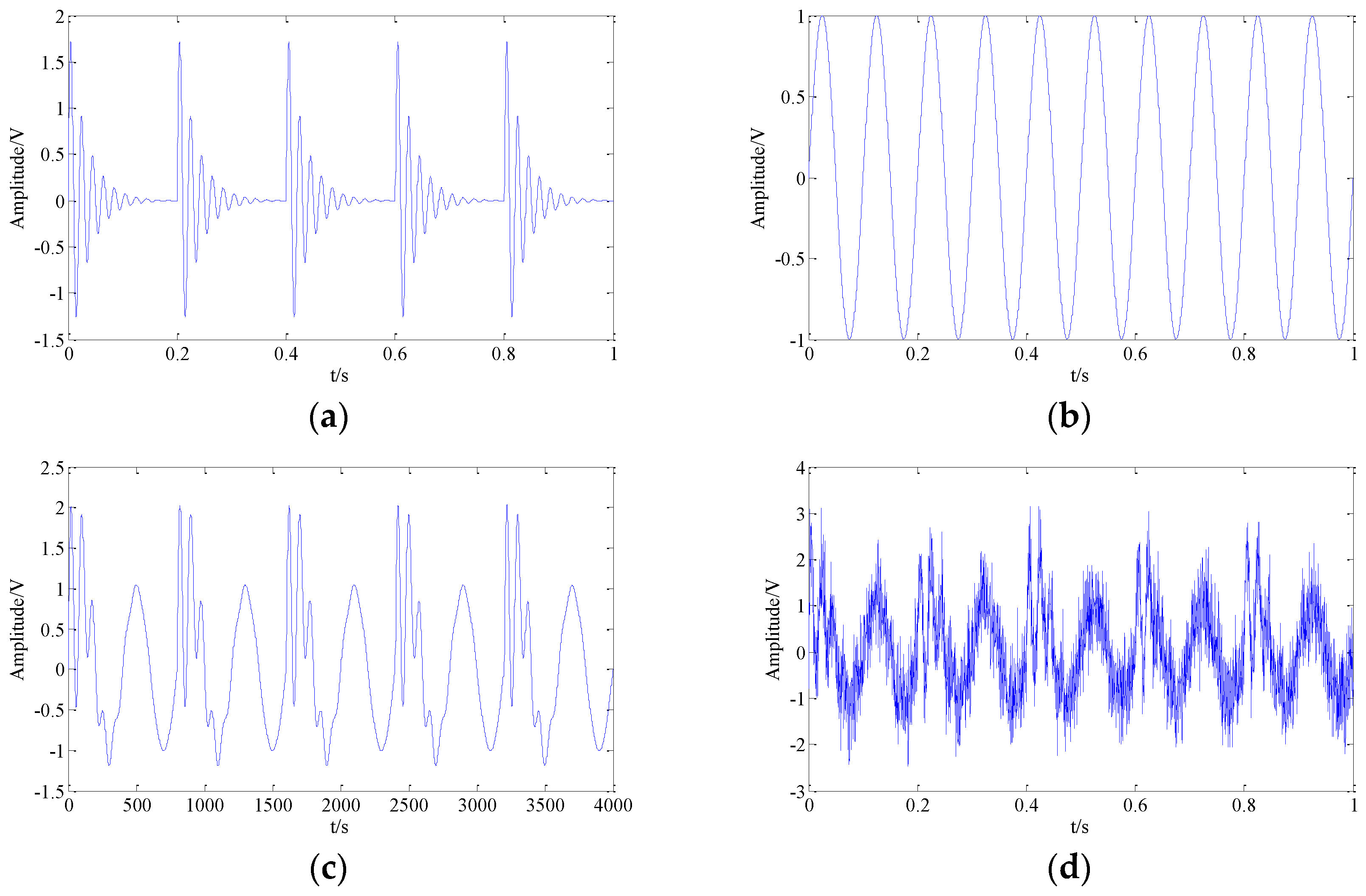
Bearings are mainly used to support rotating parts in mechanical equipment and their vibration signals always contain much information, such as fault characteristics, along with noise. The key step of fault diagnosis is an effective feature extraction of vibration signals. Commonly, the vibration signals contain harmonic components, modulation components and noise components. In order to evaluate the effectiveness of the proposed method for fault diagnosis, the simulation signals are generated as follows:

$$y(t)=x_1(t)+x_2(t)+n(t)$$

(14)

$$x_1(t)=2e^{(-0.2\pi f_{1}t)}sin(2\pi f_{1}t)$$

(15)

$$x_2(t)=sin\left(2\pi f_{2}t\right)$$

(16)

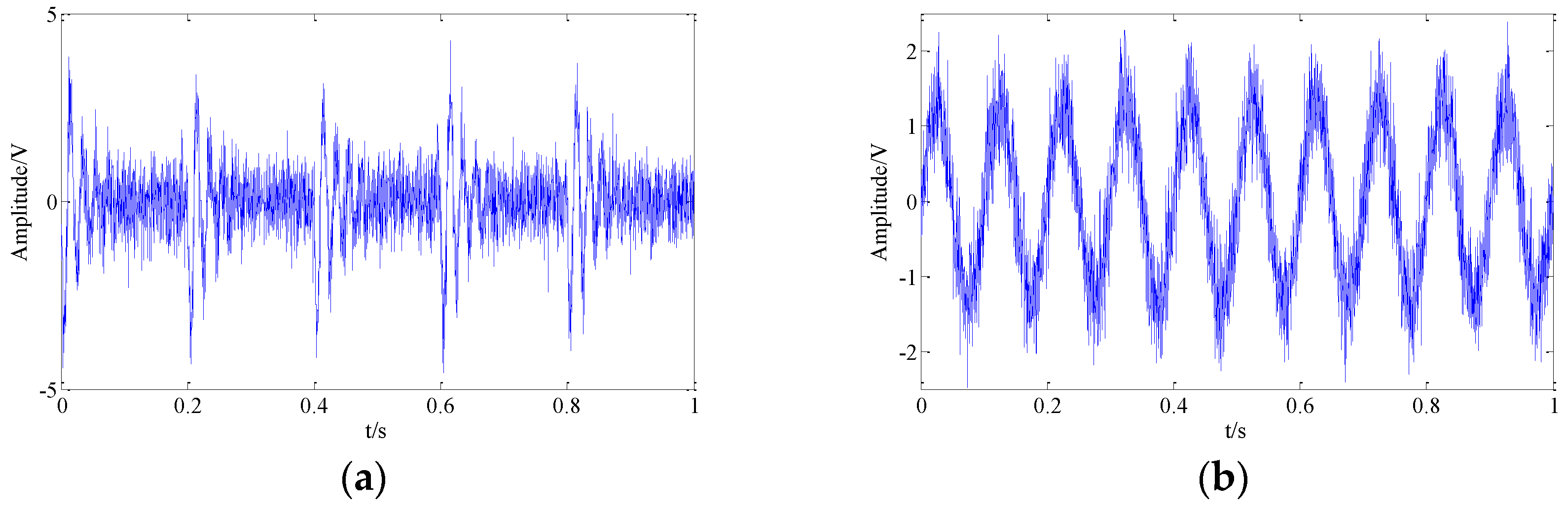
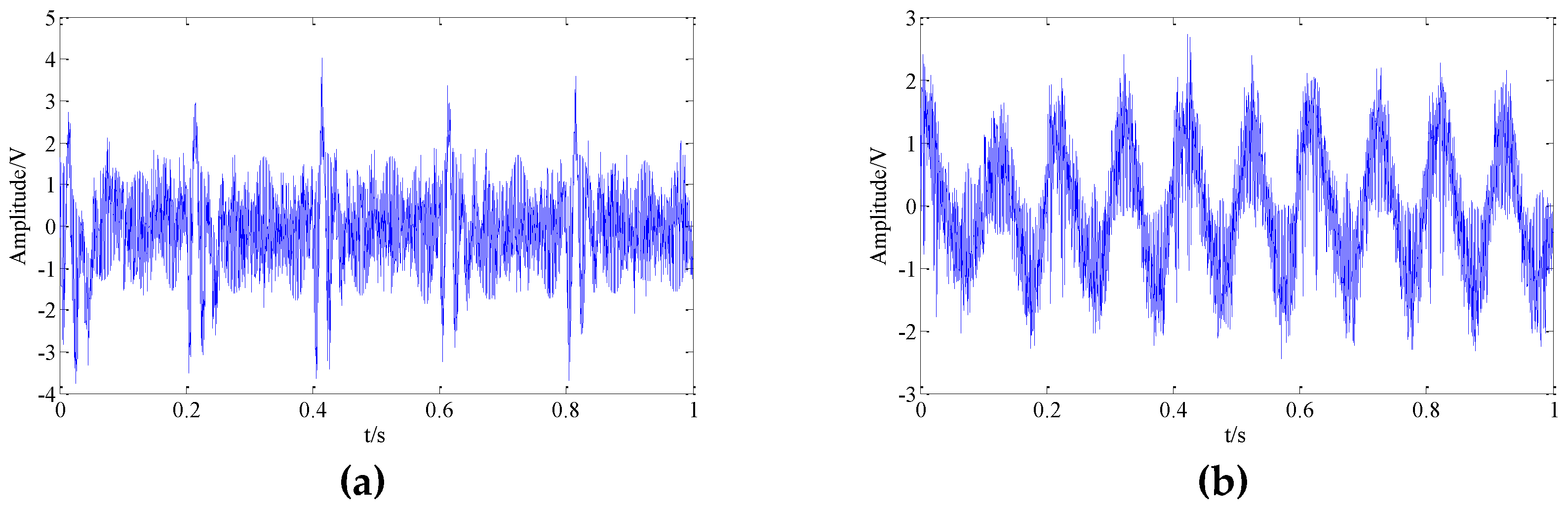
where $x_1(t)$ is the shock signal with the frequency of $f_1=50$ Hz, $x_2(t)$ is the harmonic signal with the frequency of $f_2=10$ Hz, and $n(t)$ is a Gaussian white noise with a variance of 0.5. Thus, $y(t)$ is a composite single-channel signal, which is combined by the shock signal, the harmonic signal and the noise. The sampling frequency of the signal is chosen as 6000 Hz and the sampling point is set as 4000 N. Original shock signal without noise in the time-domain is shown in Figure 4a and the harmonic signal without noise is shown as Figure 4b. Figure 4c is the composite original single-channel signal without noise in the time-domain, and Figure 4d is composite signal with noise.

According to Figure 4d, we can find that the characteristics of two constituted signals in the time-domain cannot be clearly indicated under the strong background noise. In the section of simulation signal analysis, in order to accurately evaluate the proposed method on signal reconstruction under noisy conditions, the proposed method, conventional TSSA based on CP-ALS, the traditional BSS method-Fast Independent Component Analysis (Fast-ICA) [37], and EMD-ICA are employed to the comparative analysis process.

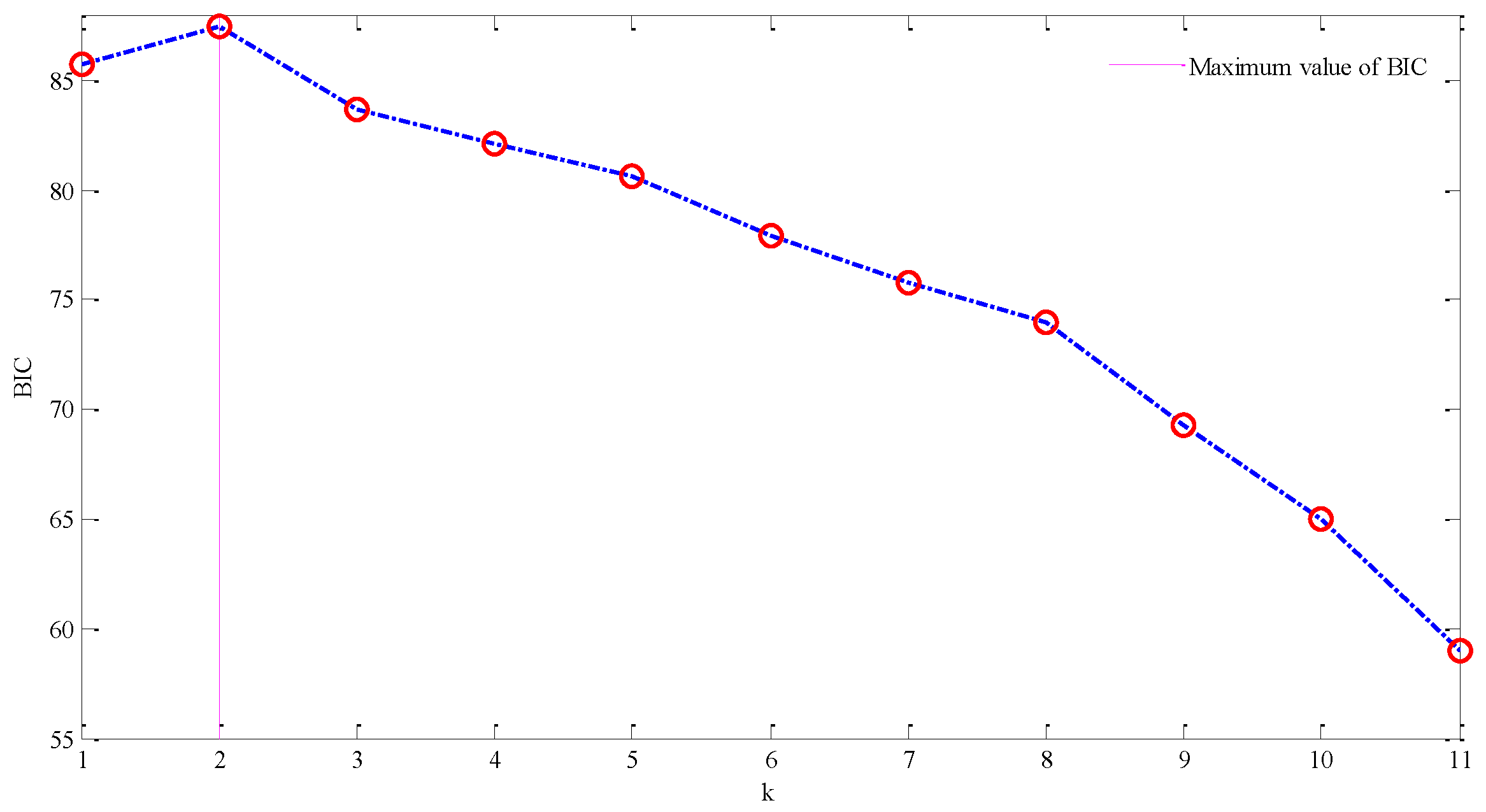
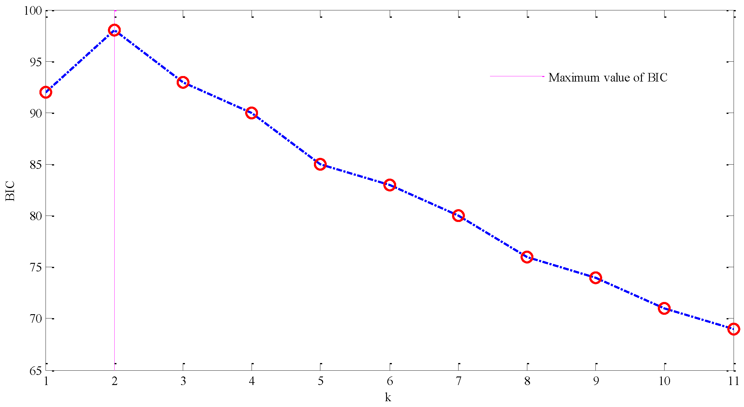
IMF_S is obtained by EMD to the measured single channel composite signal. Thus, the composite signal and the IMF_S of the decomposition can form a new multidimensional observation signal. In this way, the dimension of the observation signal can be increased, so that the new observation signal can be in accordance with the blind source separation condition. Then, we can obtain the correlation matrix about the new observation matrix, and the singular value decomposition of the correlation matrix is performed. Finally, the number of source signals can be judged further by the Bayesian information criterion. The BIC value is shown as Figure 5. According to the Figure 5, when $k=n=2$, we can obtain the maximum BIC value, which indicates the number of source signals should be 2, thus we achieve the goal of estimating the correct number of source signals.

After obtaining the number of source signals, the above-mentioned four different SCBSS methods are used to analyze the composite simulation signal. The result of Fast-ICA is shown in Figure 6, where Figure 6a presents the recovered shock signal in time-domain and Figure 6b presents the recovered harmonic signal. From the figure, it can be seen that the Fast-ICA cannot extract the shock signal and the recovered harmonic signal with noise. Hence, the Fast-ICA method is not suitable to achieve the accurate separation of composite original signal, which contains shock signal and high background noise.

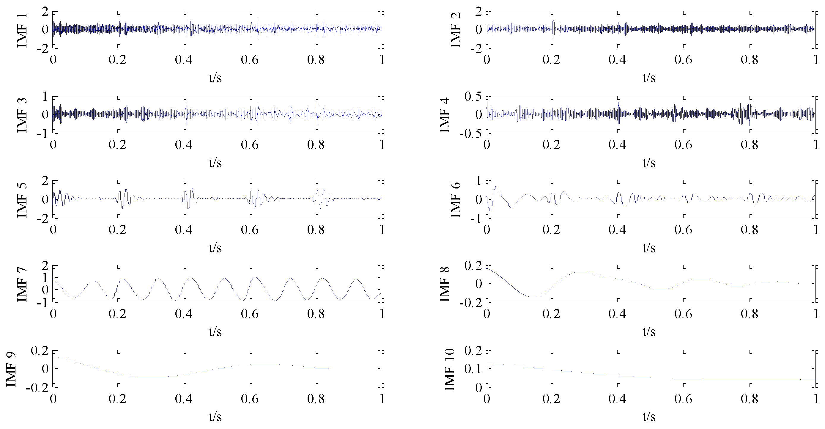
The operator of EMD is employed for the simulation signal and the result is shown in Figure 7. Firstly, several IMF_S can be obtained from the composite original signal using EMD. Then, we need to calculate the correlation coefficient between each IMFs and the original composite signal.

In

Table 1. The correlation coefficient between each IMF and the simulation signal.

IMF1	IMF2	IMF3	IMF4	IMF5	IMF6	IMF7	IMF8	IMF9	IMF10
0.052	0.043	0.003	0.352	0.203	0.311	0.806	0.086	0.056	0.069

, it can be seen that the correlation coefficient of IMF4 and IMF7 are greater than that others. Since they have large relativity with the original signal, these IMFs are chosen as the representation of source signal, and the others IMF_S belongs to unconcerned noise signal. Then, the Fast-ICA method is applied to them and the results are plotted (Figure 8). Figure 8a presents the recovered shock signal in the time-domain and Figure 8b presents the recovered harmonic signal. From the graph, it can be seen that, same as Fast-ICA, the EMD-ICA decomposition also has poor performance in extracting the shock signal and the harmonic signal. Thus, an advanced method should be developed.

Furthermore, the conventional TSSA based on CP-ALS is applied to the simulation signal. The corresponding result is plotted in the Figure 9. It is demonstrated that TSSA based on CP-ALS has better reconstruction performance than Fast-ICA and EMD-ICA. However, the reconstruction accuracy should still be improved.

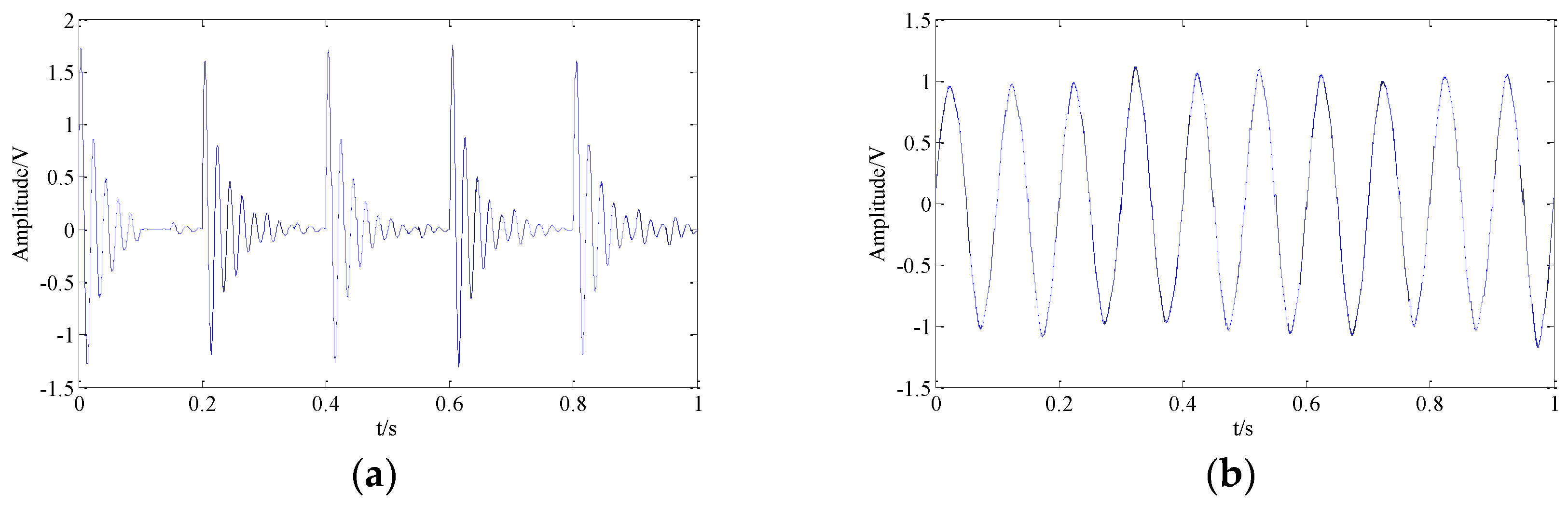
The results of proposed TSSA method based on CP-WOPT in this paper are shown in Figure 10. Figure 10a presents the recovered shock signal in the time-domain and Figure 10b presents recovered harmonic signal.

In Figure 10, it can be seen that the proposed method successfully extracts the two source signals from the composite single-channel signal. To evaluate the capacity of the proposed method more accurately, the index of similarity is chosen as the evaluation index. If the calculated value approaches 1, it indicates the extracted signal is very similar to the original signal. Otherwise, the extracted signal is not needed. After calculating the similarity between the recovered signal in Figure 10 and original signal in Figure 4, the value is close to 1, which demonstrates the advantage of proposed method for blind source separation.

4. Experimental Signal Analysis

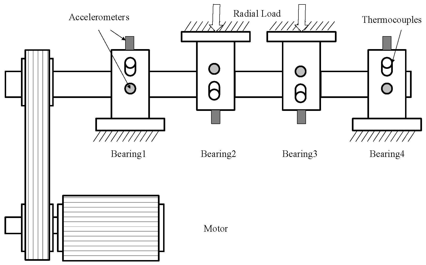
In actual operation, a bearing is an important part of rotating machinery, and the inner ring, outer ring and rolling elements are related to each other. Therefore, there is a strong correlation between the different vibration sources. Limited by the experimental conditions, only one channel observation signal is monitored. The proposed method in this paper is used to detect the coupling faults such as the inner ring, outer ring and rolling elements. The multiple-fault experimental data about bearing in this paper are provided by the University of Cincinnati, USA [38]. Experimental apparatus is shown as Figure 11. There are four Rexnord ZA-2115 double row tapered roller bearings with the circle diameter of 2.815 cm installed on the spindle, and each race has 16 rollers. The roller diameter is 0.331 cm, taper is 15.17°, the spindle Speed is 2000 r/min and the data sampling frequency is 20 kHz. The data analyzed in this paper are the No. 1 dataset in the database, in which the bearing with outer ring and inner ring fault is simulated. The fault frequencies of inner ring and rolling element in the bearing are calculated as follows:

$$f_i=\frac{n}{2}(1+\frac{d}{D}\cos \alpha )f_r$$

(17)

$$f_b=\frac{D}{2d}[1-{(\frac{d}{D})}^2{\cos }^2\alpha ]f_r$$

(18)

where $f_i$ is the characteristic frequency of the inner ring fault of rolling bearing, $f_b$ is the characteristic frequency of the rolling element fault, $f_r$ is the rotational frequency, $n$ is the number of the rolling element, $d$ is the diameter of the rolling element, $D$ is the pitch circle diameter of bearing, and α is the contact angle of rolling element. Finally, we calculate and determine the fault frequency of inner ring as $f_i=296.8$ Hz. The rolling element faulty frequency is $f_b=139.84$ Hz, and the rotational frequency is equal to $f_r=33.3$ Hz. The specific parameters of bearing are shown in

Table 2. The specific parameter of bearing.

$\mathit{d}$	$\mathit{D}$	$\mathit{n}$	α	fr	fi	fb
0.331	2.815	16	15.17°	33.33	296.8	139.84

.

To realize the blind source separation of single-channel composite signal in an experiment station, firstly, the EMD is used to decompose the composite signal, and the mode components IIMF1–IMF10 are obtained. Then, the original signal and the decomposed mode components are decomposed by SVD to obtain characteristic values. Finally, the number of source signals is determined as “2” by using the BIC, as shown in Figure 12.

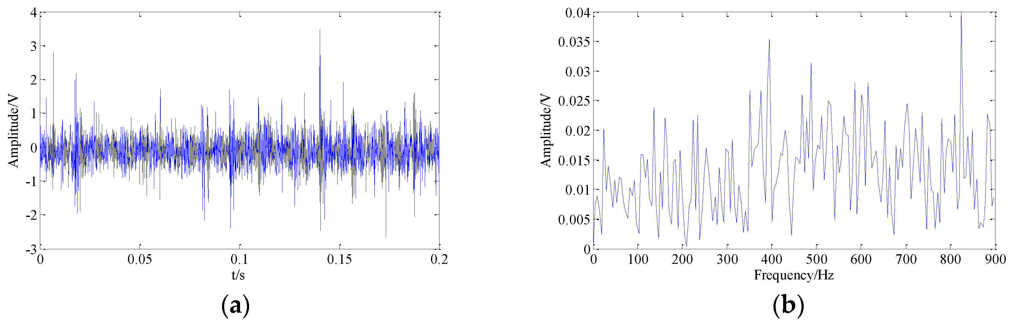
The collected composite original single-channel signals in the time-domain and the frequency-domain are shown in Figure 13a,b, respectively. According to Figure 13a, we notice that the characteristics of original signals in the time domain performance cannot be clearly identified due to the strong background noise, which makes it hard to identify whether the bearing fails and to find the location of the fault.

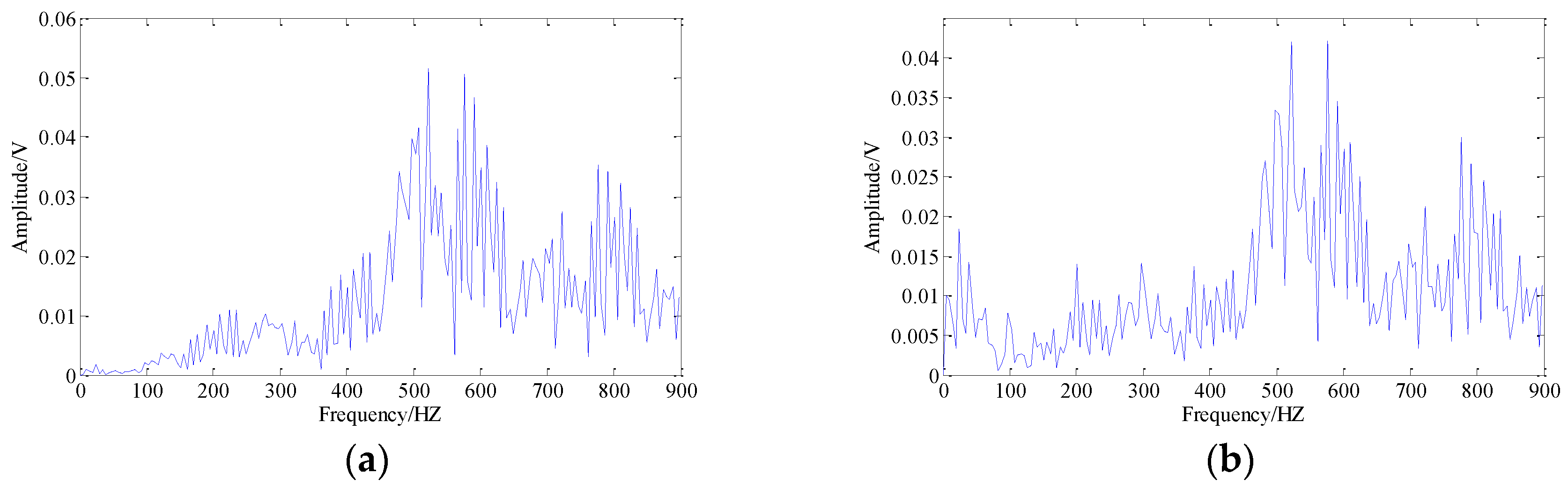
In order to accurately evaluate the effectiveness of proposed method in this paper, the EMD-ICA and the conventional TSSA based on CP-ALS are used in the comparative study. The EMD is used to decompose the composite signal, and pluralities of IMFs are obtained. Then, two IMF_S are chosen according to the maximum correlation coefficient between the IMFs and the composite signal, which can be regarded as the input data of ICA. The results are shown in Figure 14. We can make a conclusion that the recovered signals in frequency are both uncorrelated with fault frequency; therefore, the EMD-ICA is difficult to inspect the multiple faults characteristics.

Then, the conventional TSSA based on CP-ALS is employed to the measured fault signal analysis. The result is plotted in Figure 15. It is indicated that the multi-fault such as inner ring and rolling element faulty still cannot be separately identified by the conventional method.

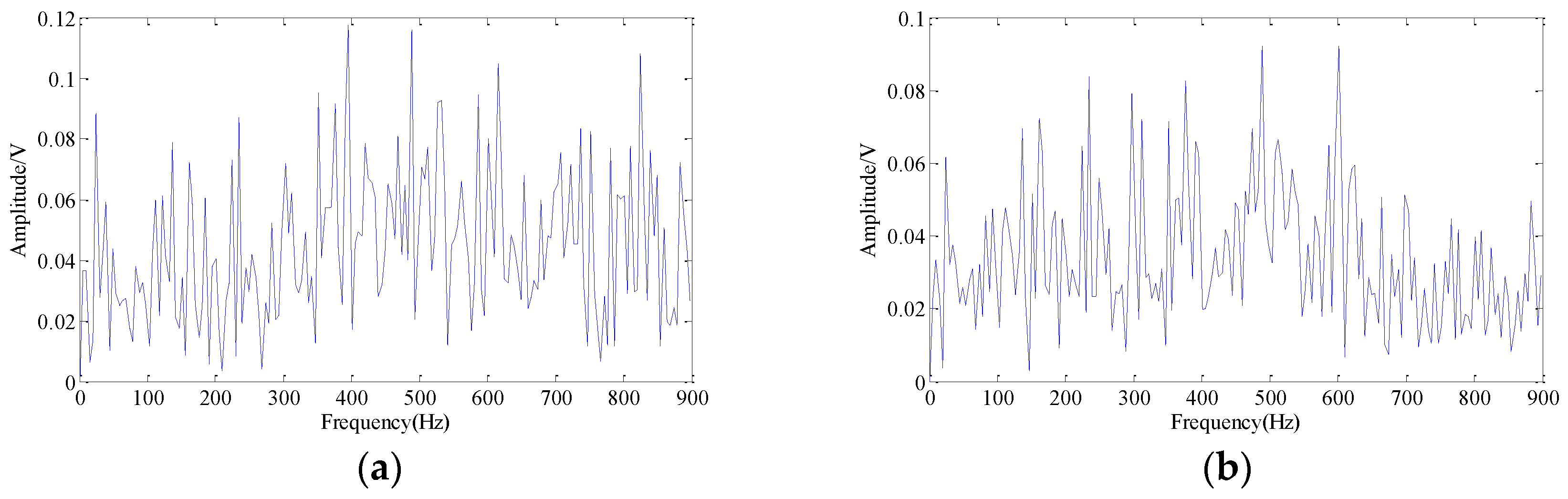
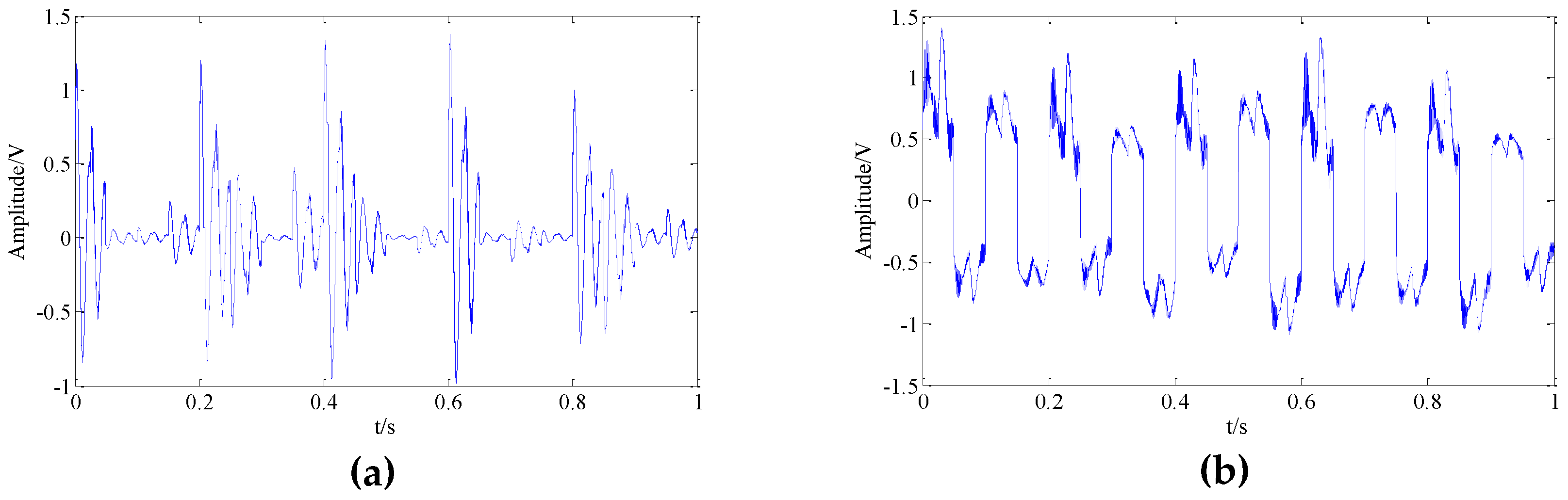
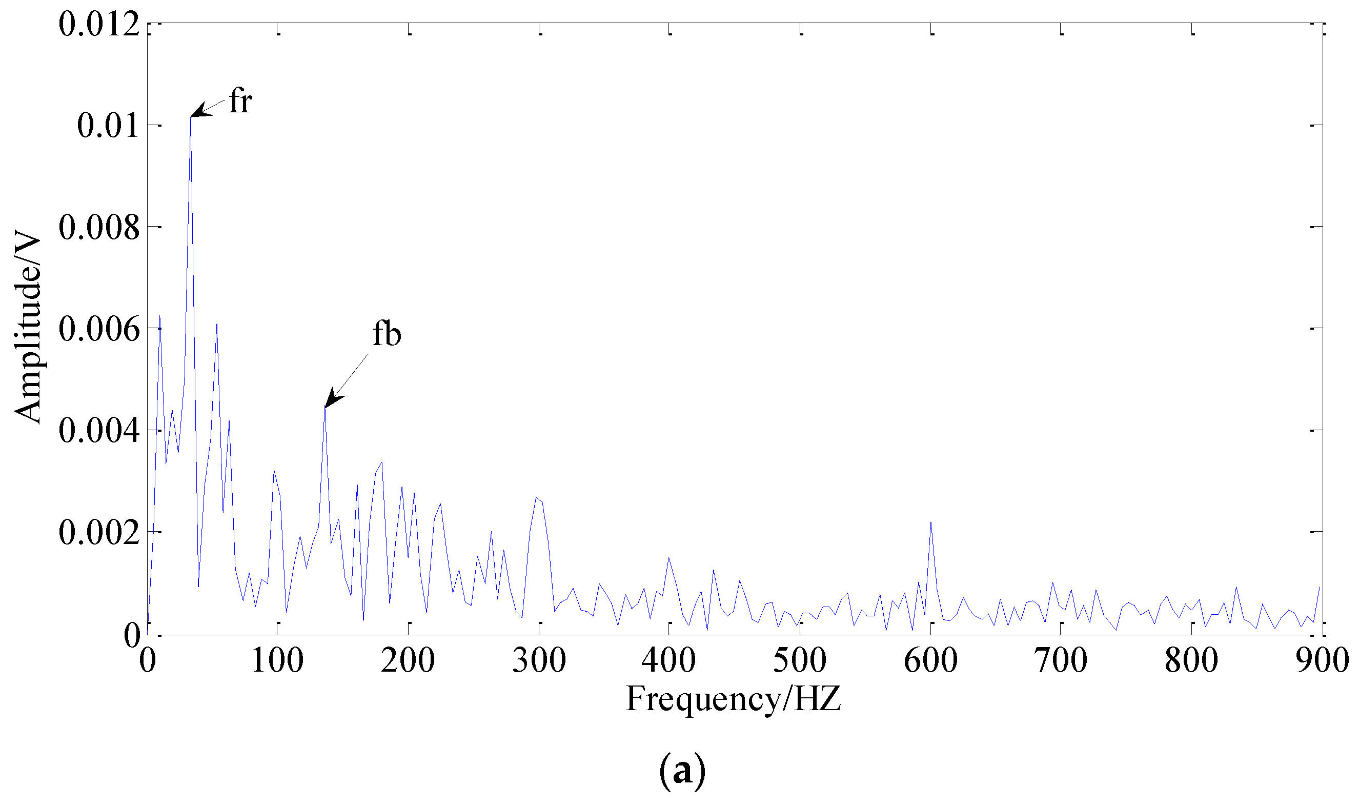
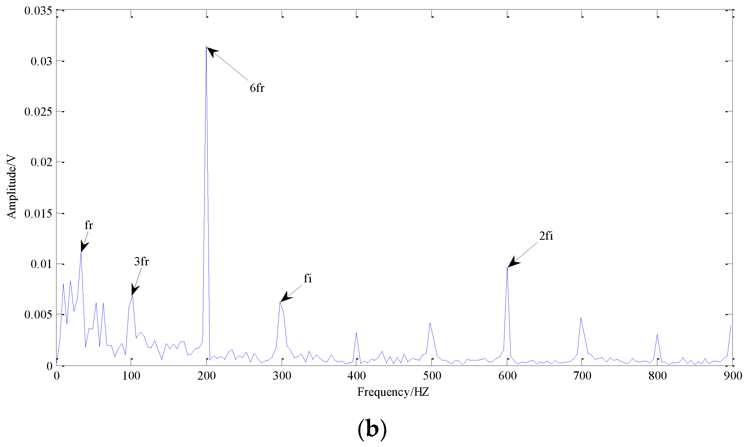
The results of the proposed TSSA method based on CP-WOPT in this paper are shown in Figure 16, where Figure 16a,b, respectively, represents the recovered No. 1 fault signal and the recovered No. 2 fault signal, all in frequency domain.

Fortunately, we can find the rotational frequency $f_r$, and the fault frequency of the rolling element f_b in Figure 16a. In Figure 16b, the rotational frequency and its frequency multiplication, the bearing fault frequency of inner ring f_i, and the twice faulty frequency of inner ring $2f_i$ can be identified. Thus, we can determine that there are two faults in the bearing: the inner ring fault and the rolling element fault. The result is consistent with the theoretical calculation [38]. Therefore, the effectiveness of proposed method for blind source separation is demonstrated, and it has obvious advantages in extracting weak multi-fault features under the strong background noise in a single-channel signal.

5. Conclusions

The blind source separation of single-channel composite signal has important theoretical significance and practical value in the extraction of multi-fault feature for mechanical equipment. The research work reported in this paper has two main contributions: firstly, a novel single channel blind source separation method using tensor-based singular spectrum analysis based on CP-WOPT is proposed, which can obtain a better convergence of tensor decomposition and a higher reliable results. Then, EMD-SVD-BIC method was introduced to estimate the number of source signals in the single-channel blind source separation. Moreover, the method is illustrated by numerical simulation signal and has an application in the analysis of faulty rolling bearing experimental signal, enabling the identification of fault source signal. It is demonstrated that the proposed method has better performance in solving SCBSS problem than the traditional signal processing methods.