A Short-Term Photovoltaic Power Prediction Model Based on an FOS-ELM Algorithm


Key Laboratory of Smart Grid of Ministry of Education, Tianjin University, Tianjin 300072, China
*
Author to whom correspondence should be addressed.
Appl. Sci. 2017, 7(4), 423; https://doi.org/10.3390/app7040423
Submission received: 8 March 2017
/
Revised: 12 April 2017
/
Accepted: 17 April 2017
/
Published: 21 April 2017
(This article belongs to the Special Issue Distribution Power Systems)
Abstract
:With the increasing proportion of photovoltaic (PV) power in power systems, the problem of its fluctuation and intermittency has become more prominent. To reduce the negative influence of the use of PV power, we propose a short-term PV power prediction model based on the online sequential extreme learning machine with forgetting mechanism (FOS-ELM), which can constantly replace outdated data with new data. We use historical weather data and historical PV power data to predict the PV power in the next period of time. The simulation result shows that this model has the advantages of a short training time and high accuracy. This model can help the power dispatch department schedule generation plans as well as support spatial and temporal compensation and coordinated power control, which is important for the security and stability as well as the optimal operation of power systems.
1. Introduction
With the fast-growing consumption of fossil fuels and the resultant environmental deterioration, we are much encouraged to use renewable energy such as solar energy, wind energy, etc. [1]. According to the statistics from the International Energy Agency [2], the global photovoltaic (PV) generation capacity growth from 2010 to 2014 has exceeded that of the last 40 years. China has been taking the lead in the global PV market since 2013, followed by Japan and the United States. Furthermore, a lower PV array price has greatly reduced the costs of building PV systems. Therefore, it is predicted that, by 2050, PV power will contribute 16% to the total energy generation capacity worldwide.
Research on PV systems may provide solutions to the many challenges faced by the environment and the power system itself. Studies have been conducted in related areas of optimizing the energy structure and of improving the performance of a PV system. Despite the advantages mentioned above, a PV system is highly subject to environment pollution, and has been criticized for its unstable, random and intermittent power output [3].
When a PV system is connected to the grid, its power fluctuation may destabilize the grid and pose a threat to network security, which makes it even harder to formulate generation plans. As such, an accurate prediction of PV power output is required to make better generation plans, support the spatial and temporal compensation, and achieve coordinated power control, so that the need for energy storage capacity and operating costs can be reduced [4]. Moreover, better prediction of PV power also helps to enhance system security and stability, as well as optimize the operation of the power system [5]. The prediction methods include physical methods and statistical methods. Usually, a physical method first predicts the factors which directly influence the PV power output (such as solar radiation and ambient temperature) and then uses the forecast result as the input of the physical model to obtain the output power. On the other hand, a statistical method uses historical data to build a statistical model based on some machine learning algorithms, and predicts the PV power output directly without building a specific physical model.
It has been proved that the physical method is superior to the statistical method, given large data sets [6]. Some regression models are also used to figure out the relationship between the input and output variables, such as the random forest model [7] and the support vectors regression model [8]. Researchers have built many kinds of neuron networks to predict the power production of PV systems. For example, Li has proposed an improved gray prediction model [9]. Also, the radial basis function (RBF) network has been applied to this area [10]. In another paper [11], they use a back propagation (BP) neural network to solve the prediction problem.
In recent years, many hybrid methods have been proposed, which combine the advantages of both methods. In reference [12], a hybrid approach was developed to forecast short-term solar PV power based on the combination of the wavelet transform (WT) and radial basis function neural network (RBFNN). Some researchers also combined the seasonal auto-regressive integrated moving average method (SARIMA) and the support vector machines (SVM) method [13]. These models are proved to be effective in PV prediction, although many of them, such as SVM and RBFNN models, are complicated in terms of computation and very data-intensive for the network.
All the models reviewed above ignored the time validation of the data, and assumed the data would not be out-of-date. In actual practice, training data are time sensitive, so the training data need to be updated in real time. Only a few published research papers have considered this fact so far. Among them, an online 24-h prediction model was proposed, which used an RBF network and classified the input variables based on the weather type [14]. Some researchers have described a two-stage method where a statistical normalization of the solar power is first obtained, and then the forecasts of the normalized solar power are calculated to predict the PV power [15].
We chose to employ the extreme learning machine (ELM) algorithm because of the following advantages:
- (1)
- The computation complexion of ELM is much lower than many other machine learning algorithms.
- (2)
- The learning speed of ELM is much faster than most feed forward network learning algorithms.
- (3)
- The generalization performance of ELM is better than many others.
- (4)
- The amount of hidden layer nodes is small and they do not need to be tuned [16].
The aim of our work was to develop a simple and accurate online model for forecasting the power produced by a PV power plant. In order to achieve this goal, we built the prediction model based on the online sequential extreme learning machine with forgetting mechanism (FOS-ELM), which predicts the PV power output for the next 15 min in a rolling manner.
The main contributions of our work are summarized below:
- We introduced an online learning model with a Forgetting Mechanism to the area of photovoltaic prediction, which can update the data in real time.
- We compared the ELM, OS-ELM and FOS-ELM prediction models in predicting PV power in different seasons.
- The simulation results showed that the FOS-ELM model can not only improve the accuracy but also reduce the training time.
2. Prediction Algorithm
2.1. Classical Extreme Learning Machine (ELM)
The ELM is a single hidden-layer artificial neural network. It is assumed that the number of random hidden neurons in the ELM model is L, and the number of different learning samples is N. It is also assumed that , , , , and , and are randomly generated matrices and vectors, respectively. Then, the output function can be rewritten as:
where is the output weight vector, which connects the random hidden neurons with the output. is the active function, which connects the random hidden neuron with all of the input nodes, and can be any infinitely differentiable function, such as the Sigmoid function as shown below:
Equation (1) can be written in the form of matrices, such as:
where
Then, the least-square solution of (1) is:
where the matrix is the hidden layer output matrix, within which the element () is the hidden layer output vector for input . is the vector of the output of the training data. is the only parameter for the training process to determine. The upper bound of the required number of hidden nodes is the number of distinct training samples, in other words, the number of hidden nodes should be less than the number of training samples.
To improve the stability and generalizability of the results, we added the regularization parameter C to (4) to transform it as [18]:
2.2. Online Sequential ELM (OS-ELM)
The classical ELM assumes that all the data (samples) are used for training, but in the prediction model, the data is coming chunk-by-chunk (a block of data) or one-by-one (the latter can be seen as a special condition of the former). Therefore, the classical ELM should be adjusted to such conditions [19]. In the PV power prediction model, historical weather and PV power data are collected from the Supervisory Control And Data Acquisition (SCADA) system periodically. As OS-ELM updates the training data on time, it is more suitable for the PV power prediction. The algorithm is shown as follows.
Step 1: Initialization—use a chunk of training data as initial data.
- (a)
- Randomly generate and where .
- (b)
- Calculate the initial hidden layer output matrix .
- (c)
- Estimate the initial output weight vector:where
- (d)
- Set .
Step 2: Online study.
- (a)
- When the chunk of new data is ready,
- (b)
- Calculate the partial hidden layer output matrix based on the latest data.
- (c)
- Estimate the new and based on (7) and (8).
- (d)
- Set , and then go back to Step 2.
2.3. OS-ELM with Forgetting Mechanism (FOS-ELM)
In practice, training data are time sensitive. In other words, data are only valid within a certain time period. In the process of the FOS-ELM, the data obtained earlier than a certain time can no longer be used under the forgetting mechanism, since the outdated data may make the prediction less accurate [20]. As solar radiation and temperature vary seasonally, the FOS-ELM is more appropriate for the PV power prediction model. The algorithm of FOS-ELM is presented as follows.
Step 1: Initialization, which is the same as Step 1 in the OS-ELM.
Step 2: Online learning with the forgetting mechanism.
When the chunk of new data is ready,
- (a)
- Calculate the partial hidden layer output matrix , which corresponds to the latest data.
- (b)
- Estimate the new and based on (9) and (10).
- (c)
- Set , and then go back to Step 2.
It is obvious that the difference between FOS-ELM and OS-ELM is the addition of the forgetting mechanism, which can not only get rid of the outdated data to avoid their interference in the training networks, but also can reveal the timeliness of the data.
3. Model Architecture
3.1. Physical Model
The output power of a PV array can be calculated by [21]:
where is the transform efficiency; S is the size of the PV array (m2); R is the solar radiation (kW/m2); e is the loss in efficiency of the array for every degree Celsius of cell temperature increase (always equals to 0.005); and is the ambient temperature (°C).
As shown in (11), the output power is affected by several factors, including the transform efficiency, PV array size, solar radiation and ambient temperature.
3.2. Input Vector
Based on the physical model presented in Section 3.1, we identified the factors that influence the output power. For a certain array, the efficiency and the size are fixed, as included in the historical data. However, the solar radiation and ambient temperature change with time periodically. Therefore, we choose time, solar radiation and ambient temperature as the input parameters. The input data is obtained from a numerical weather predilection (NWP) model, which uses mathematical models of the atmosphere and oceans to predict the weather on current weather conditions [22]. The input vector is:
where is the ambient temperature, and is the amount of solar radiation reaching the part of the Earth’s surface near the photovoltaic cells.
3.3. Data Pre-Processing
We then normalize the different variables to adapt to the ELM in the following way:
where is the input or output data, while and are the maximum and minimum of the value.
As the measurement results cannot be exactly accurate, the measured power production and solar radiation data can sometimes be less than zero due to measurement errors, which is impossible in actual practice. In this case, we tune them and the corresponding predicted data to zero. When we calculate the errors, we will eliminate the data set where the measured and predicted values are both equal to zero.
3.4. Error Evaluation
The normalized Root Mean Square Error () and Mean Absolute Percent Error () are used to evaluate the prediction methods, which are calculated as follows:
where is the number of time periods for power generation; is the rated power; is the predicted power in the time period; and is the measured power in the time period. In order to avoid the nighttime data, we disregarded the data set where both the solar radiation and PV generated power data are equal to zero.
3.5. Flowchart of the Model
The prediction process is illustrated in Figure 2.
First, we input the initial historical data for pre-processing, generate the initial hidden layer output matrix , and estimate and . Then, we input the weather forecast data of the next period of time and calculate the prediction value. When the historical data such as the weather and power data arrive, we calculate the prediction error and save the data. After that, we check the time. If it is equal to 1 h, we update the matrices , and ; otherwise, the above process is repeated.
4. Examples and Simulation
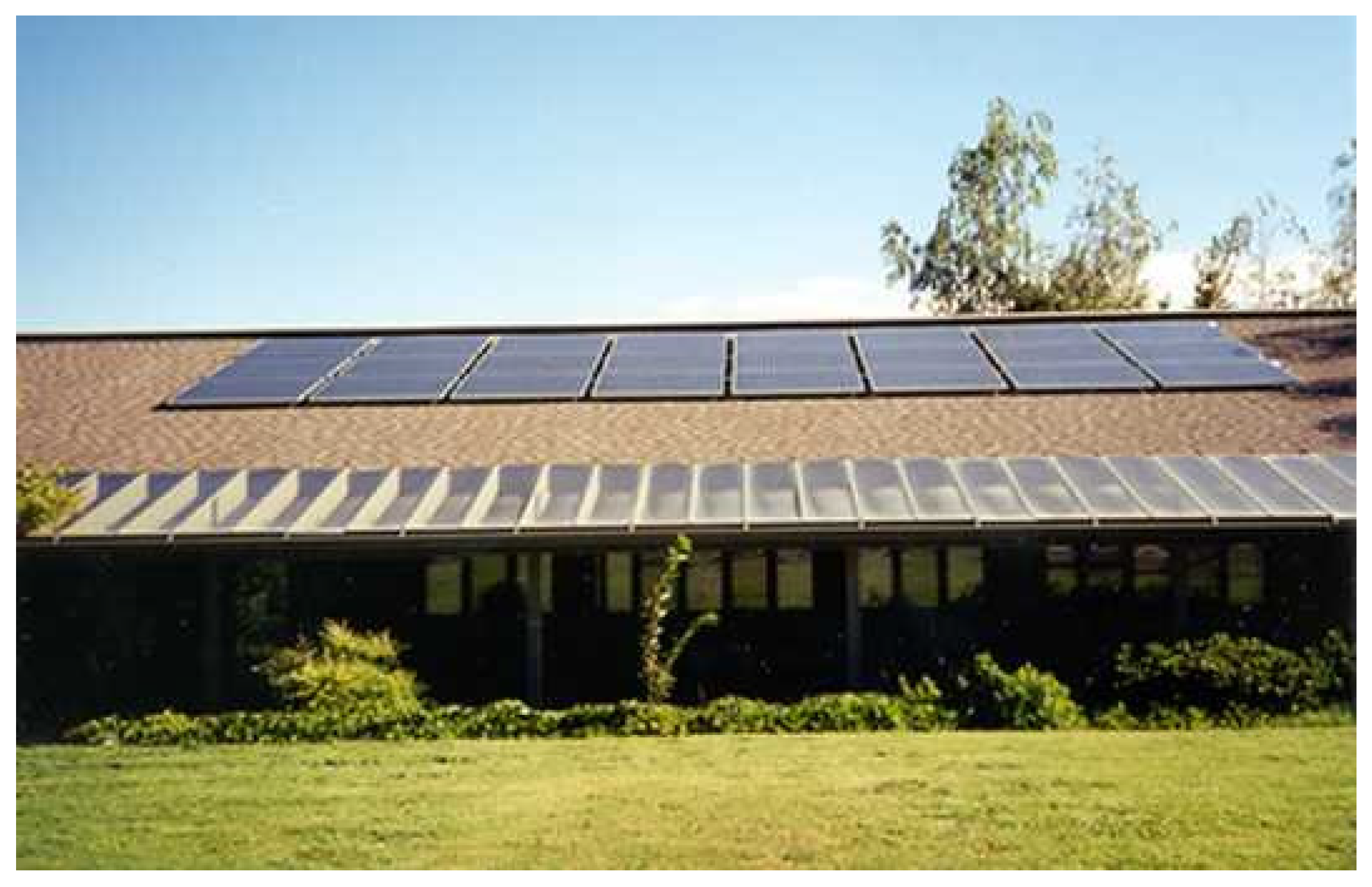
In this paper, we used the data from the solar power plant in Ashland, Oregon, with the capacity of 5 kW, downloaded from the website of [23], to simulate the proposed FOS-ELM-based prediction model and compare it with the OS-ELM and ELM models. The plant faces south, tilted 15 degrees. As the paper has shown, the training time and prediction accuracy (in terms of and ) of the ELM method are better than the BP neural networks [24], so we therefore focus on the comparison of ELM, OS-ELM and FOS-ELM.
The 5 kW solar electric arrays are located on the roof of the Ashland Court House, which is shown in Figure 3.
The details of the three models are presented as follows:
Model 1 (FOS-ELM Algorithm): The sigmoid function was chosen as the active function; the data obtained at 48 h ahead of the current time (from 6:00 to 18:00, every 15 min) was used as the training data to predict the power output; the training sample was updated every one hour and then the data obtained 48 h ago was dropped.
Model 2 (OS-ELM Algorithm): The sigmoid function was chosen as the active function; the data obtained at 48 h ahead of the current time (from 6:00 to 18:00, every 15 min) was used as the training data to predict the power output; the training sample was updated every one hour with the earlier data remaining.
Model 3 (ELM Algorithm): The sigmoid function was chosen as the active function; the data obtained within the last 48 h of the last month (from 6:00 to 18:00, every 15 min) was used as the training data to predict the power output. In other words, the model was retrained every month.
We set the number of hidden layer neurons as 120.
4.1. Accuracy Comparison in a Single Day
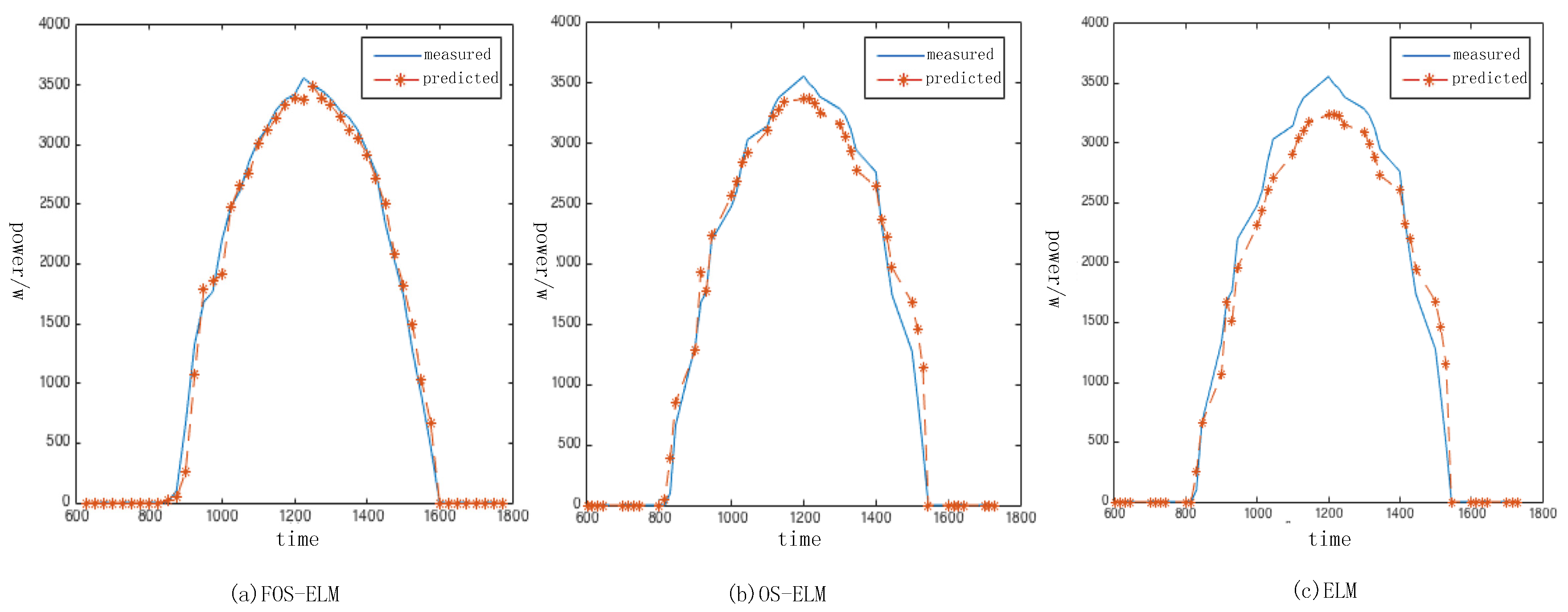
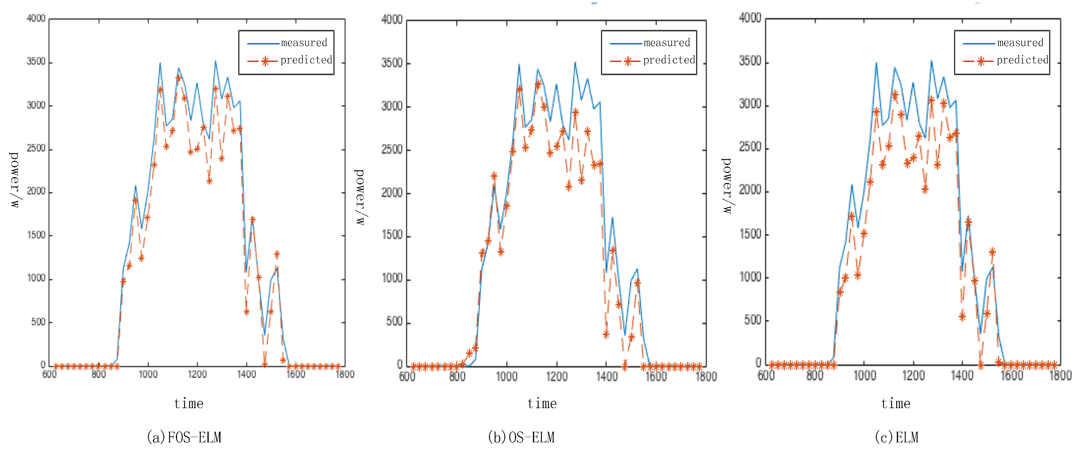
A comparison of the prediction results of the three models during a certain sunny day in January in 2015 is shown in Figure 4, where 600 on the X-axis stands for 6:00.
The of models 1, 2 and 3 are 0.023, 0.035 and 0.053, respectively; the corresponding are 9.707, 10.893 and 12.706. It is obvious that the accuracy of Model 1 is the best among the three models.
A certain cloudy/rainy day in January in 2015 is also used to compare the prediction results of the three models, as shown in Figure 5.
The of models 1, 2 and 3 are 0.067, 0.074 and 0.082, respectively; the corresponding are 13.833, 14.303 and 15.112. It is obvious that the accuracy of Model 1 is still the best among the three models.
4.2. Monthly Average Accuracy Comparison
To compare the accuracy of the three models in different seasons, we choose the data in Spring (from April to June), Summer (from July to September), Autumn (from October to December) and Winter (from January to March) for testing. The results are shown in Table 1.
We can see from Table 1 that, in terms of , the prediction accuracy is higher in Winter and Summer than in Autumn and Spring; among the three models, Model 1 has the highest accuracy while Model 3 is the lowest. In terms of , the prediction accuracy is higher in Summer than in Winter; again, the accuracy of Model 1 is the highest and that of Model 3 the lowest. In a nutshell, the FOS-ELM method proves to have the best performance.
4.3. Comparison of Training Time
The three models were run in MATLAB. In Model 1, it takes 0.095 s for initialization and 0.052 s for online study. In Model 2, it takes the same time as that of Model 1 to initialize, but only 0.049 s for online study. It takes 0.076 s to train each time in Model 3. Therefore, it can be seen that online study can save about 30% of retraining time. However, it takes 6% more time in Model 1 than in Model 3 for every time online study is conducted.
5. Conclusions
In this paper, we proposed a new short-term PV power prediction model based on the FOS-ELM method. First of all, we gave a brief introduction to the theories of ELM, OS-ELM, FOS-ELM, and analyzed the differences between the three models to explain why FOS-ELM is the best one to predict PV power generation, in theory. After that, we built our prediction system that is ready to be applied in practice. Finally, in the simulation part, we used the data provided by the University of Oregon Solar Radiation Monitoring Laboratory to test our models. The proposed FOS-ELM model showed shorter training time and higher accuracy than the classical ELM and OS-ELM models, in all seasons and weather conditions.
Acknowledgments
The authors greatly acknowledge the support from National Natural Science Foundation of China (NSFC) (51477111) and National Key Research and Development Program of China (2016YFB0901102).
Author Contributions
Jidong Wang conceived the idea of the study and conducted the research. Ran Ran analysed most of the data, and wrote the initial draft of the paper. Yue Zhou contributed to refining the ideas, carrying out additional analyses and finalizing this paper.
Conflicts of Interest
The authors declare no conflicts of interest.
References
- Paravalos, C.; Koutroulis, E.; Samoladas, V.; Kerekes, T.; Sera, D.; Teodorescu, R. Optimal Design of Photovoltaic Systems Using High Time-Resolution Meteorological Data. IEEE Trans. Ind. Inform. 2014, 10, 2270–2279. [Google Scholar] [CrossRef]
- IEA. Technology Roadmap, Solar Photovoltaic Energy. Available online: http://www.iea.org/ (accessed on 10 July 2016).
- Paatero, J.V.; Lund, P.D. Effects of large-Scale photovoltaic power integration on electricity distribution networks. Renew. Energy 2007, 32, 216–234. [Google Scholar] [CrossRef]
- Bortolini, M.; Gamberi, M.; Graziani, A. Technical and economic design of photovoltaic and battery energy storage system. Energy Convers. Manag. 2014, 86, 81–92. [Google Scholar] [CrossRef]
- Mohamed, A.; Eltawil, M.A.; Zhengming, Z. Grid-Connected photovoltaic power systems: Technical and potential problems—A review. Renew. Sustain. Energy Rev. 2010, 14, 112–129. [Google Scholar]
- Graditi, G.S.; Ferlito, S.; Adinolfi, G. Comparison of Photovoltaic plant power production prediction methods using a large measured dataset. Renew. Energy 2016, 90, 513–519. [Google Scholar] [CrossRef]
- Zamo, M.; Mestre, O.; Arbogast, P.; Pannekoucke, O. A benchmark of statistical regression methods for short-term forecasting of photovoltaic electricity production. Part II: Probabilistic forecast of daily production. Sol. Energy 2014, 105, 792–803. [Google Scholar] [CrossRef]
- Baharin, K.A.; Abd Rahman, H.; Hassan, M.Y.; Gan, C.K. Hourly Photovoltaics Power Output Prediction for Malaysia Using Support Vector Regression. Appl. Mech. Mater. 2015, 785, 591–595. [Google Scholar] [CrossRef]
- Li, Y.; Zhang, J.; Xiao, J.; Tan, Y. Short-Term prediction of the output power of PV system based on improved gray prediction model. In Proceedings of the IEEE International Conference on Advanced Mechatronic Systems, Kumamoto, Japan, 10–12 August 2014; pp. 547–551. [Google Scholar]
- Al-Amoudi, A.; Zhang, L. Application of radial basis function networks for solar-Array modelling and maximum power-Point prediction. IEE Gener. Transm. Distrib. 2000, 147, 310–316. [Google Scholar] [CrossRef]
- Shang, X.X.; Chen, Q.J.; Han, Z.F.; Qian, X.D. Photovoltaic super-Short term power prediction based on bp-Ann generalization neural network technology research. Adv. Mater. Res. 2013, 791, 1925–1928. [Google Scholar] [CrossRef]
- Mandal, P.; Madhira, S.T.S.; Haque, A.U.; Meng, J.; Pineda, R.L. Forecasting Power Output of Solar Photovoltaic System Using Wavelet Transform and Artificial Intelligence Techniques. Procedia Comput. Sci. 2012, 12, 332–337. [Google Scholar] [CrossRef]
- Bouzerdoum, M.A.; Mellit, A.; Pavan, A.M. A hybrid model (SARIMA–SVM) for short-Term power forecasting of a small-Scale grid-Connected photovoltaic plant. Sol. Energy 2013, 98, 226–235. [Google Scholar] [CrossRef]
- Chen, C.; Duan, S.; Cai, T.; Liu, B. Online 24-h solar power forecasting based on weather type classification using artificial neural network. Sol. Energy 2011, 85, 2856–2870. [Google Scholar] [CrossRef]
- Bacher, P.; Madsen, H.; Nielsen, H.A. Online short-Term solar power forecasting. Sol. Energy 2009, 83, 1772–1783. [Google Scholar] [CrossRef]
- Huang, G.B.; Zhu, Q.Y.; Siew, C.K. Extreme learning machine: A new learning scheme of feed forward neural networks. In Proceedings of the IEEE International Joint Conference on Neural Networks, Budapest, Hungary, 25–29 July 2004; pp. 985–990. [Google Scholar]
- Huang, G.B.; Zhou, H.; Ding, X.; Zhang, R. Extreme learning machine for regression and multiclass classification. IEEE Trans. Syst. Man Cybern. B Cybern. 2012, 42, 513–529. [Google Scholar] [CrossRef] [PubMed]
- Huang, G.B.; Chen, L.; Siew, C.K. Universal approximation using incremental constructive feedforward networks with random hidden. IEEE Trans. Neural Netw. 2006, 17, 879–892. [Google Scholar] [CrossRef] [PubMed]
- Liang, N.Y.; Huang, G.B.; Saratchandran, P.; Sundararajan, N. A fast and accurate online sequential learning algorithm for feed forward networks. IEEE Trans. Neural Netw. 2006, 17, 1411–1423. [Google Scholar] [CrossRef] [PubMed]
- Zhao, J.W.; Wang, Z.; Dong, S.P. Online sequential extreme learning machine with forgetting mechanism. Neurocomputing 2012, 87, 79–89. [Google Scholar] [CrossRef]
- Riffonneau, Y.; Bacha, S.; Barruel, F.; Ploix, S. Optimal Power Flow Management for Grid Connected PV Systems With Batteries. IEEE Trans. Sustain. Energy 2011, 2, 309–320. [Google Scholar] [CrossRef]
- Lynch, P. The origins of computer weather prediction and climate modeling. Comput. Phys. 2008, 227, 3431–3444. [Google Scholar] [CrossRef]
- University of Oregon Solar Radiation Monitoring Laboratory. Available online: http://solardat.uoregon.edu/SelectDailyTotal.html (accessed on 9 May 2016).
- Li, Z.; Zang, C.; Zeng, P.; Yu, H. Day-Ahead hourly photovoltaic generation forecasting using extreme learning machine. In Proceedings of the IEEE International Conference on Cyber Technology in Automation, Control, and Intelligent Systems IEEE, Shenyang, China, 8–12 June 2015; pp. 779–783. [Google Scholar]
Figure 1.
The architecture of Extreme Learning Machine.
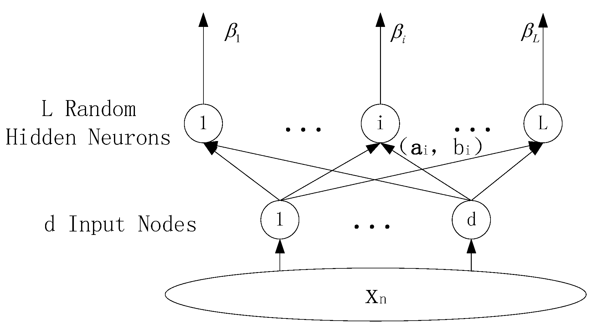
Figure 2.
Flowchart of the online sequential extreme learning machine with forgetting mechanism (FOS-ELM) prediction model.
Figure 2.
Flowchart of the online sequential extreme learning machine with forgetting mechanism (FOS-ELM) prediction model.
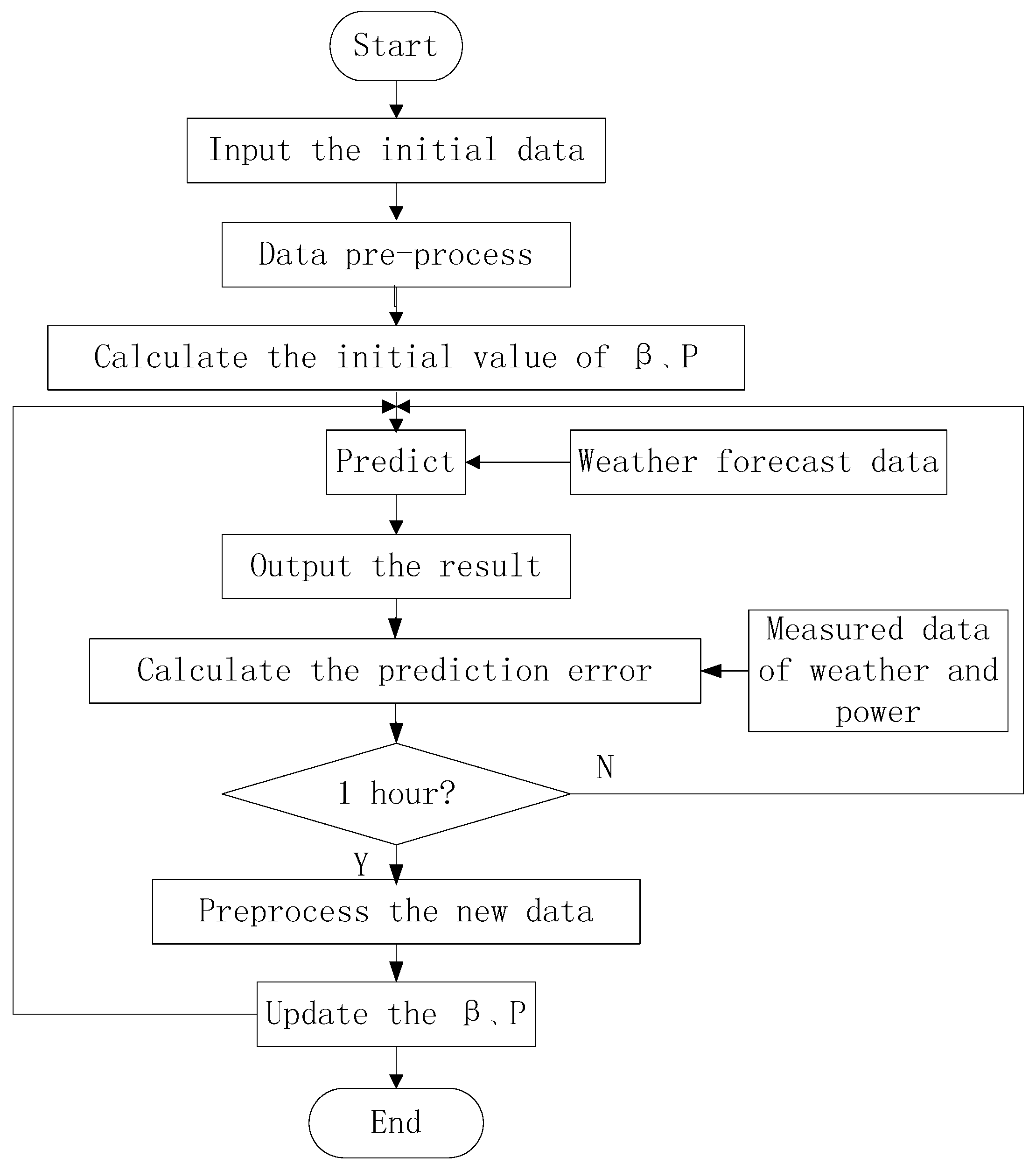
Figure 3.
The 5 kw solar electric arrays on the roof of the Ashland Court House.

Figure 4.
Comparison of three models on a sunny day. (a) FOS-ELM; (b) online sequential extreme learning machine (OS-ELM); (c) extreme learning machine (ELM).
Figure 4.
Comparison of three models on a sunny day. (a) FOS-ELM; (b) online sequential extreme learning machine (OS-ELM); (c) extreme learning machine (ELM).

Figure 5.
Comparison of three models on a cloudy/rainy day. (a) FOS-ELM; (b) OS-ELM; (c) ELM.


Table 1.
Monthly average accuracy comparison.
| Season | Model | /% | |
|---|---|---|---|
| Spring (Apri–June) | FOS-ELM | 0.0953 | 15.492 |
| OS-ELM | 0.1041 | 16.730 | |
| ELM | 0.1126 | 18.483 | |
| Summer (July–September) | FOS-ELM | 0.0892 | 14.329 |
| OS-ELM | 0.0933 | 15.883 | |
| ELM | 0.1083 | 16.032 | |
| Autumn (October–December) | FOS-ELM | 0.0974 | 15.289 |
| OS-ELM | 0.1018 | 16.325 | |
| ELM | 0.1219 | 17.933 | |
| Winter (January–March) | FOS-ELM | 0.0876 | 15.245 |
| OS-ELM | 0.0945 | 16.319 | |
| ELM | 0.0983 | 17.703 |
© 2017 by the authors. Licensee MDPI, Basel, Switzerland. This article is an open access article distributed under the terms and conditions of the Creative Commons Attribution (CC BY) license (http://creativecommons.org/licenses/by/4.0/).
Share and Cite
MDPI and ACS Style
Wang, J.; Ran, R.; Zhou, Y. A Short-Term Photovoltaic Power Prediction Model Based on an FOS-ELM Algorithm. Appl. Sci. 2017, 7, 423. https://doi.org/10.3390/app7040423
AMA Style
Wang J, Ran R, Zhou Y. A Short-Term Photovoltaic Power Prediction Model Based on an FOS-ELM Algorithm. Applied Sciences. 2017; 7(4):423. https://doi.org/10.3390/app7040423
Chicago/Turabian StyleWang, Jidong, Ran Ran, and Yue Zhou. 2017. "A Short-Term Photovoltaic Power Prediction Model Based on an FOS-ELM Algorithm" Applied Sciences 7, no. 4: 423. https://doi.org/10.3390/app7040423
Note that from the first issue of 2016, this journal uses article numbers instead of page numbers. See further details here.