
A New Robust Tracking Control Design for Turbofan Engines: H∞/Leitmann Approach


1
College of Energy and Power Engineering, Nanjing University of Aeronautics and Astronautics, Nanjing 210016, Jiangsu, China
2
The George W. Woodruff School of Mechanical Engineering, Georgia Institute of Technology, Atlanta, GA 30324, USA
*
Author to whom correspondence should be addressed.
Appl. Sci. 2017, 7(5), 439; https://doi.org/10.3390/app7050439
Submission received: 28 December 2016
/
Revised: 10 April 2017
/
Accepted: 19 April 2017
/
Published: 27 April 2017
Abstract
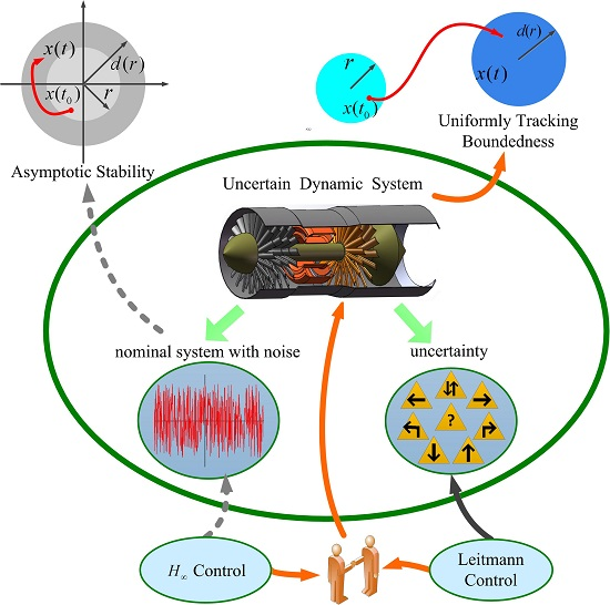
:In this paper, a /Leitmann approach to the robust tracking control design is presented for an uncertain dynamic system. This new method is developed in the following two steps. Firstly, a tracking dynamic system with simultaneous consideration of parameter uncertainty and noise is modeled based on a linear system and a reference model. Accordingly, a “nominal system” from the tracking system is defined and controlled by a control to obtain the asymptotical stability and noise resistance. Secondly, by making use of a Lyapunov function and the norm boundedness, a new robust control with the “Leitmann approach” is designed to cope with the uncertainty. The two controls collaborate with each other to achieve “uniform tracking boundedness” and “uniform ultimate tracking boundedness”. The new approach is then applied to an aircraft turbofan control design, and the numerical simulation results show the prescribed performances of the closed-loop system and the advantage of the developed approach.

1. Introduction
The performance indicators of aircraft, such as thrust weight ratio, economic efficiency and control performance, raise higher requirements for aircraft engines [1,2,3]. These requirements bring the need for more adjustable variables in the engines, which means the engine control system has multi-inputs and multi-outputs. Coupling inherently exists among these inputs and outputs. Moreover, the nonlinear characteristics of aircraft engines is another problem to be solved in its control design. This nonlinearity results from the engine thermodynamic characteristics and the variety of its initial and operating conditions. One can investigate the nonlinearity by a component-level thermodynamic model, what we called the nonlinear model. For the engine control design, most of the researchers build a linear model, such as a state space variable model (SSVM) based on the nonlinear model, which will cause modeling error during the linearization. The parameters in the SSVM may be disturbed by airflow distortion or other devices. At the same time, due to the mechanical manufacture and the assembly, there exists a difference between individual engines, which results in the parameter disturbance of the SSVM. All of these problems—couplings, nonlinearity, modeling errors, parameter perturbation and individual difference—present researchers with challenges on the control design for an aircraft turbofan.
In order to conquer the mentioned problems in the aircraft engine control, researchers have been putting great efforts into the methods of robust control. The linear quadratic regulator (LQR) method has strong robustness and a simple structure, which was applied to the F100 aircraft engine and other linear systems [4,5]. In the multivariable control of the F100, the LQR method was utilized to design the proportional part of the control. While the LQR method relies on a nominal linear system model and needs to know all of its states, if nonlinearity, uncertainty and modeling errors, which cause the remarkable mismatch between the dynamics of real systems and their models, exist, the characteristics of the LQR controller will deteriorate evidently. As was mentioned in [4], if the gain of LQR controller was not in the gain schedule, the system stability was unable to be guaranteed. To solve the problem that the LQR method cannot be utilized with the lack of partial states, the linear quadratic gaussian(LQG) method adopts the Kalman filter as a state observer to estimate the states and realize the state feedback control [6,7]. However, the Kalman filter weakens the robustness. The simulation in [6] shows that since the engine dynamics changes significantly due to the low temperature reaction in the combustion process, the performance of the LQG controller becomes worse. In [7], for the dynamics of homogeneous charge compression ignition (HCCI) engines remains invariant, the robustness of the discrete-time LQG methods cannot be verified sufficiently. To enhance the robustness of the LQG method, the loop transfer recovery (LTR) design is added to achieve the LQG/LTR approach for a linear system [8,9]. In [9], a non-full recovering LQG/LTR approach is applied to a turbofan engine. No uncertainty nor noise are considered in the controller design, and the system is actually a nominal system. The performance of the LQG/LTR controller is only validated at one operating condition, namely, km, . When facing a complicatedly-varying dynamics, such as the dynamics of turbofan engines, the LQG/LTR controller may hardly recover the transfer function desired. The control theory attracts many researchers in robust control design, especially in the noise elimination by setting a disturbance rejection level from noises to outputs. The research works in this field are numerous [10,11,12,13]. The proportion integral derivative (PID) control method is practically applied to turbofan engines; while the three parameters, proportional, integral and differential, need to be adjusted at different operating conditions [14,15]. This brings the drawbacks that the parameters of the controller are numerous and the parameter adjustment lacks a theoretical support.
In this paper, we explore a new robust tracking control design from two points of view. Firstly, the nonlinearity, coupling, modeling error, parameter disturbances and individual differences in turbofan control systems are described as the uncertainty. The new robust control approach is developed for an dynamic system with the uncertainty and the noise. Secondly, the tracking controller design will be based on the new performances, uniform tracking boundedness (UTB) and uniform ultimate tracking boundedness (UUTB). They are actually looser performances than the asymptotical stability achieved by the above-mentioned robust controls and may be more practical for a system with complicated dynamics, such as aircraft engines. The robust controller based on the new performances can ensure that system responses track reference commands and the tracking errors are bounded.
For solving the uncertainty problems, little a priori knowledge of the uncertainty and few performance indicators to constrain the effects of uncertainty were adopted in the aforementioned methods. Taking advantage of the uncertainty characteristics, including the structure matching conditions and the upper-bound of uncertainty, Leitmann and his collaborators defined the uniform boundedness (UB) and uniform ultimate boundedness (UUB), the performances for an uncertain dynamic system, and initiated the efforts of corresponding robust control designs [16,17,18]. Here, we call it the Leitmann approach. This robust control design takes the upper-bound of the uncertainty norm and the principle of the Min-Max Lyapunov function into account and assured the system responses within a certain neighborhood of the zero state. The Leitmann approach was developed into the centralized and decentralized robust control of the uncertain linear or nonlinear system with the time delay, no structure matching conditions or coupling [19,20,21], and it was applied to robust controls of the flexible structures, the switched systems and the robot manipulation [22,23,24,25]. Moreover, researchers attempted the combination between the Leitmann approach and the other control theory to enhance the controller ability and enrich the performance of the closed system. Lu utilized the principle of the Min-Max Lyapunov function and the estimation of the uncertainty bound to obtain the UUB under a slide mode control [26]. The marriage between the Leitmann method and the the fuzzy theory was explored in [27,28,29]. The fuzzy bound of the uncertainty and a delicate defuzzification are considered to obtain a deterministic robust control. We notice that most of the research with the Leitmann approach was on the problem of a state regulator design, and little attempt was made in tracking control research, which is realistic in the real world. For instance, when a pilot pulls/pushes the throttle lever or changes the flight altitude, the commands to a turbofan control system will change continuously. The system measurements need to track the varying commands, and a tracking control with high performances is necessary in this case.
Making good use of the merits of the Leitmann method and the classic robust control theory, an /Leitmann approach for a tracking control is proposed. In Section 2, we establish a linear model with the noise and the uncertainty, as well as a reference model for a uncertain dynamic system. The reference model helps to realize a tracking control system. The new tracking control scheme is presented with two steps in Section 3. First, according to the investigation of the uncertain system, we define a nominal system, which consists of the noise, but the uncertainty. An controller was designed to reduce the influence of noises and guarantees the asymptotical stability of the nominal system. Secondly, we design a robust control with the Leitmann method, which was combined with the control to yield the new performances, uniform tracking boundedness (UTB) and uniform ultimate tracking boundedness (UUTB). In Section 4, the /Leitmann approach is applied to the multi-variable tracking control design of a turbofan. The nominal system is obtained based on its component thermodynamic model [30], and the uncertainty covers the dynamic nonlinearity, the parameter disturbance, the modeling errors and the individual difference. The computer simulation results show that the resulting control can guarantee the desired tracking performances with respect to the noise and the uncertainty.
2. Problem Statement
Consider an uncertain system with uncertainty and noise described by:
Here, is time, is the state, is the control input, is the noise and is the output. , , , , , are known constant real matrices; is a matrix function representing time-varying parameter uncertainties in the system model and proposed by the following assumption.
Assumption .
There exist real matrices and , such that:
for all .
Define:
From (1), can be considered as the whole uncertain element.
Assumption .
Consider that the uncertain system (1) subjected to Assumption 1, for all , satisfies:
where is the maximum value of , is the maximum value of and is a known function.
Consider a reference model described as:
where , and are, respectively, the state, input and the output of the reference model. By (1) and (3), we have a deviation system as:
where , , are the state, control input and output of the uncertain system. For the robust control design, we divide the system (4) into two parts: the nominal system (the system without the uncertainty) and the uncertain portion. Consider System (4); we propose our robust control as:
where is the control for the nominal system and is the control for the uncertain portion. We describe the nominal system as:
where , are the state and output of the nominal system (1).
Assumption .
There is a continuous non-negative function and a continuous strictly-increasing functions , , which satisfy:
that for all , such that:
Now, we propose define our tracking performances as follow.
Definition 1.
Uniform tracking boundedness: Consider a linear dynamic system:
and a reference dynamic system:
where , , , and are known constant real matrices and . The tracking dynamic system is defined as:
where .
If and , is a solution of (15), then:
where:
and:
Furthermore, the solution has a continuation over .
Definition 2.
Uniform ultimate tracking boundedness: Consider the system (15), and is its solution. If , there exist R and , such that:
where:
and:
Remark 1.
In most of the previous research, the state regulation, but the tracking control, was studied, and the main performances are about the state, not the dynamic tracking error. Here, we present Definitions 1 and 2 as the performances for a tracking control system.
3. Controller Design
3.1. Robust Control Design for the Nominal System
For the nominal system (6), we design a controller. Let:
where is the gain of the controller.
Define:
Here, , are constant real matrices. By (23), the system (6) can be rewritten as:
Theorem 1.
Consider System (24); for a given scalar , if the matrices and W exist, such that:
then we can solve , the gain of the controller of System (24) [30], as:
Then, there is a Lyapunov function of System (24) written as:
where:
Remark 2.
It is worth noticing that the determinate of the positive matrix X is greater than zero, which implies that X is invertible.
Proof of Theorem 1.
See Appendix A. ☐
3.2. Design of /Leitmann Control for the Uncertain System
Under the controller (22) and (26) of the nominal System (24), we get a basic performance of the system (8). Then, we further investigate the design of the robust control . By introducing (22) and (23) into (6), we have:
Here, is determined by Theorem 1.
Define:
We present the robust control as:
Here, is a given scalar.
Now, by the preparation given above, we are ready to propose our main result as Theorem 2.
Theorem 2.
Consider the uncertain dynamic system (29) subject to Assumptions 1–3. Under the control (7), (22) and (31), the solution of the resulting controlled system has the performance of uniform tracking boundedness and uniform ultimate tracking boundedness.
Proof of Theorem 2.
See Appendix B. ☐
4. Application to Turbofan Engines
4.1. Control System of Turbofan Engines
Consider an aircraft turbofan engine shown in Figure 1, which consists of the fan, the compressor, the combustor, the high pressure turbine( HPT), the low pressure turbine (LPT), the mixing chamber, the afterburner and the exhaust nozzle. The numbers in Figure 1 denote the main sections of the turbofan, which are taken as the subscript of the related signals, such as the exhaust nozzle area .
As an air-breath engine, the air is inhaled into the inlet of the turbofan and compressed by the fan and the compressor. The high-pressure air flows into the combustor and gets mixed with fuel. The mixed gas is ignited and burned in the combustor. The burned gas with high temperature and pressure drives the HPT and LPT, which connect to the compressor and the fan through the high-pressure rotation spool and the low-pressure rotation spool, respectively. By this mechanical connection, the HPT and LPT transfer the power to the fan and compressor. The thrust of the turbofan is determined by the velocities of the turbofan input air and output gas and the exhausting pressure of nozzle. For the modern aircraft turbofan, the fuel flow rate and are selected to control and , the rotational speeds of the low-pressure spool and the high-pressure spool, and to realize the indirect control of the thrust. By employing perturbation techniques at each equilibrium condition, a set of linear state variable models (SVM) that depict the interactions of the engine states with inputs and outputs is established. Consequently, the turbofan can be described as (4), and:
where is the rotational speed of the low-pressure spool, is the decreasing pressure ratio of the turbine, is the main fuel flow and is the exhaust nozzle area. The reference model (5) can be specified by:
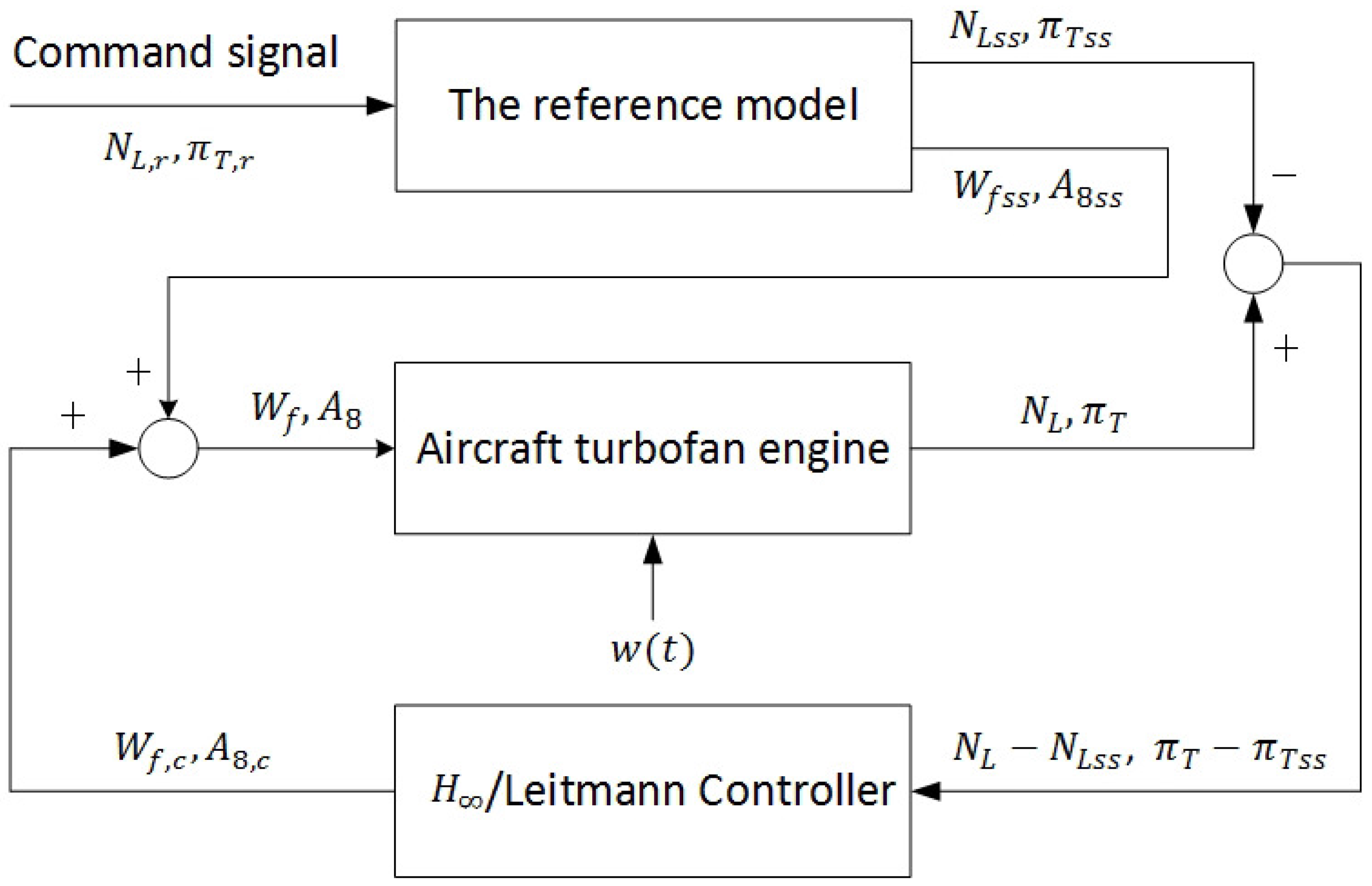
where , , , are corresponding parameters of the reference model. The new control scheme of this turbofan is depicted in Figure 2. In this control scheme, the reference model receives the commands and outputs the reference states and control forces, which combine with the engine states and control forces to form signals of the tracking system, such as . The /Leitmann controller takes the tracking errors as inputs and gives the outputs, which collaborate with the outputs of the reference model, to obtain the final control forces for the engine. It is worth noticing that the reference model has two contributions here. First of all, it provides the reference tracking trajectory for the states of the engine. Secondly, its control forces guarantee the baseline of controls for the engine, which will enhance the stability of the controlled system.
4.2. Numerical Simulation
For the numerical simulation, generally we extract a linear model from a turbofan nonlinear system by the small perturbation method and the fitting method at some operating condition. This nonlinear system is modeled based on the component thermodynamic and experiment data. In this paper, only the linear model will be discussed for the control design, and the more detailed modeling procedure of the turbofan nonlinear system can be seen in [31]. By the above-mentioned methods, we obtained a linear model at km, with:
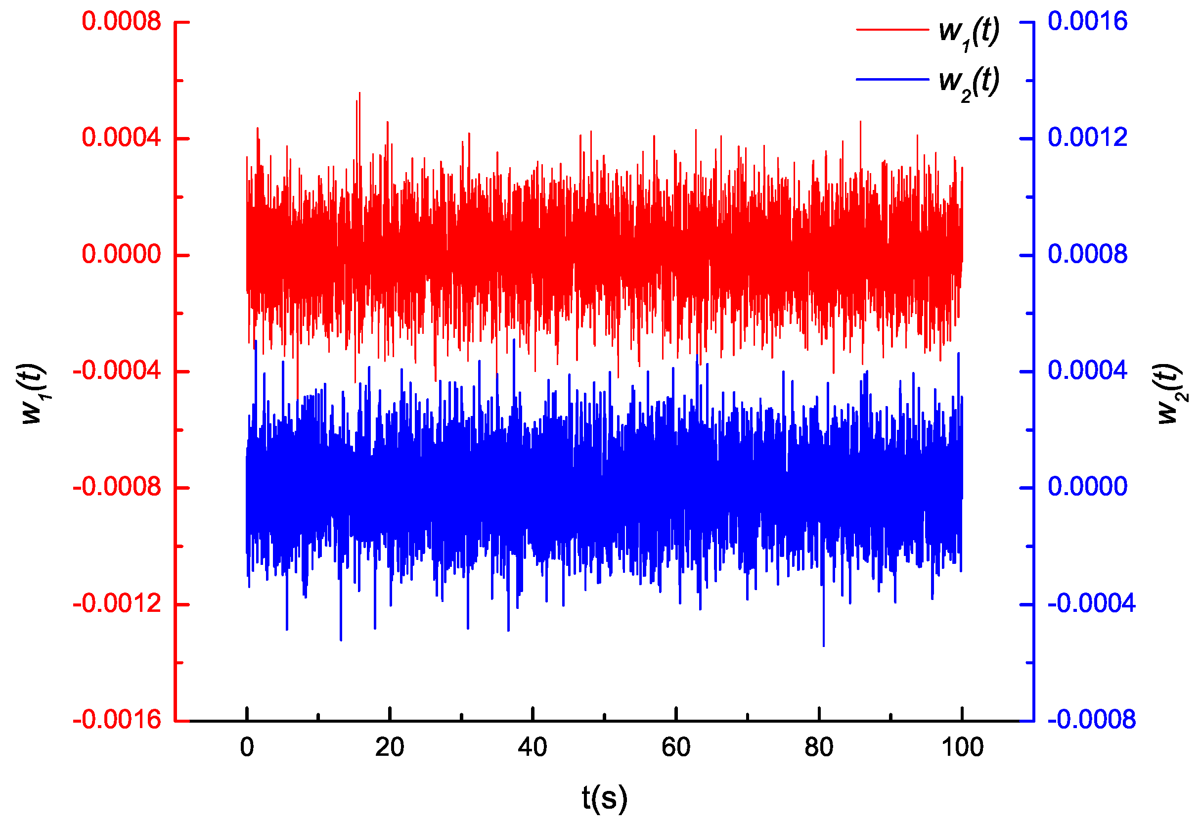
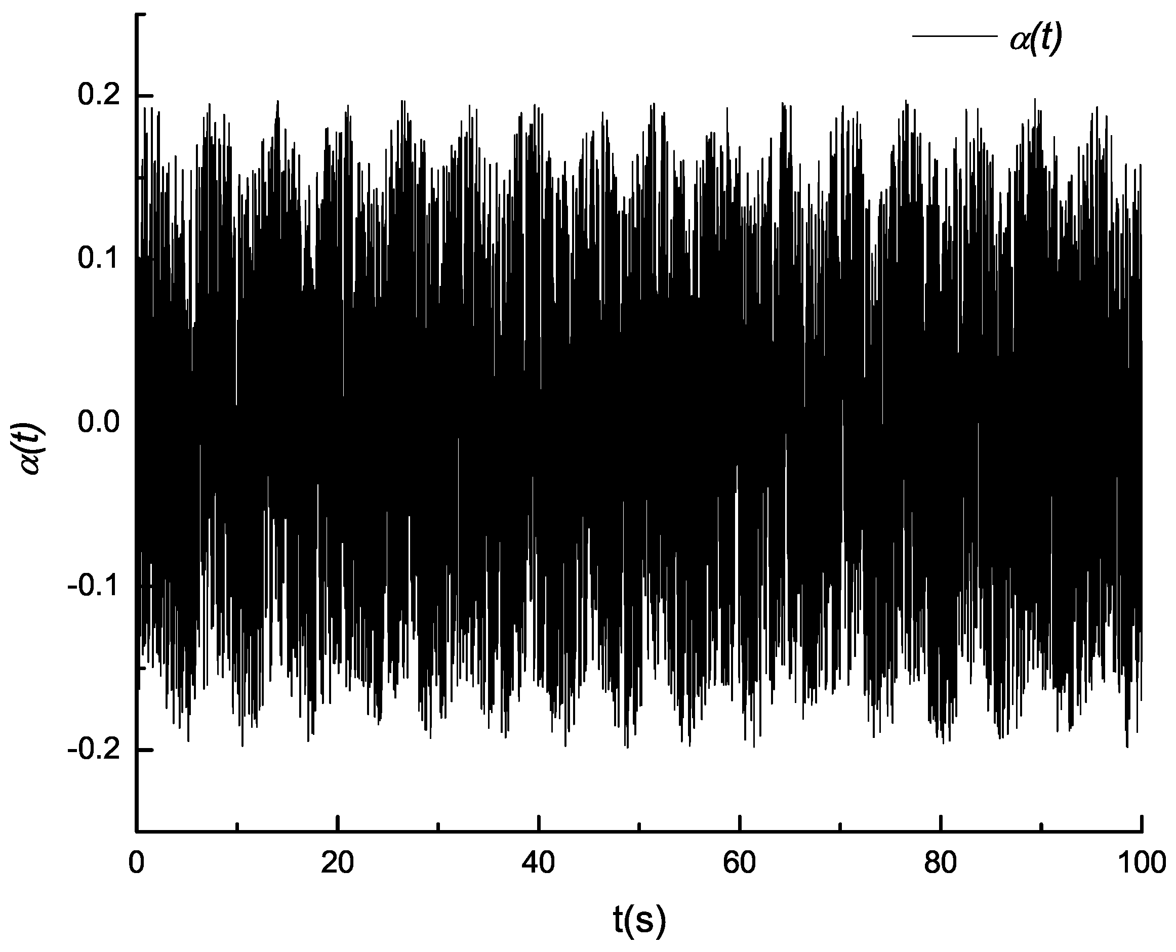
Let and:
where is a random number and is a sine function. By simple calculation, we know . Let , and is a white noise with zero expectation. The noise and the uncertainty are shown in Figure 3 and Figure 4.
For the nominal system of the turbofan, we solve the linear matrix inequations (LMIs) in (25) and obtain the following gain matrices:
Let , and can be written as:
where:
Finally, by (7), (38), (39) and (40), the /Leitmann control is:
Choose:
Here, and are the minimum and maximum eigenvalues of a matrix. By solving the LMIs in (25), we have , and .
At the same time, to compare the robustness between our developed approach and an applied robust control, we designed a controller with the LQR method, which was used to obtain a multivariable control law on an F100 engine system [4]. The LQR control is:
Let , and then, the controller gain matrix is:
Apply the controller (41), controller (38) and LQR controller (42) to the system (4) with (36) and (37). Let and , the commands of and , step in the magnitude of , and , separately, and the responses of states and control inputs are shown in Figure 5, Figure 6, Figure 7, Figure 8, Figure 9, Figure 10, Figure 11, Figure 12, Figure 13 and Figure 14 and in Table 1 and Table 2.
4.3. Analysis and Comparison of the Simulation Results
In this section, we intend to analyze and compare the simulation results of state responses under the above-mentioned controllers.
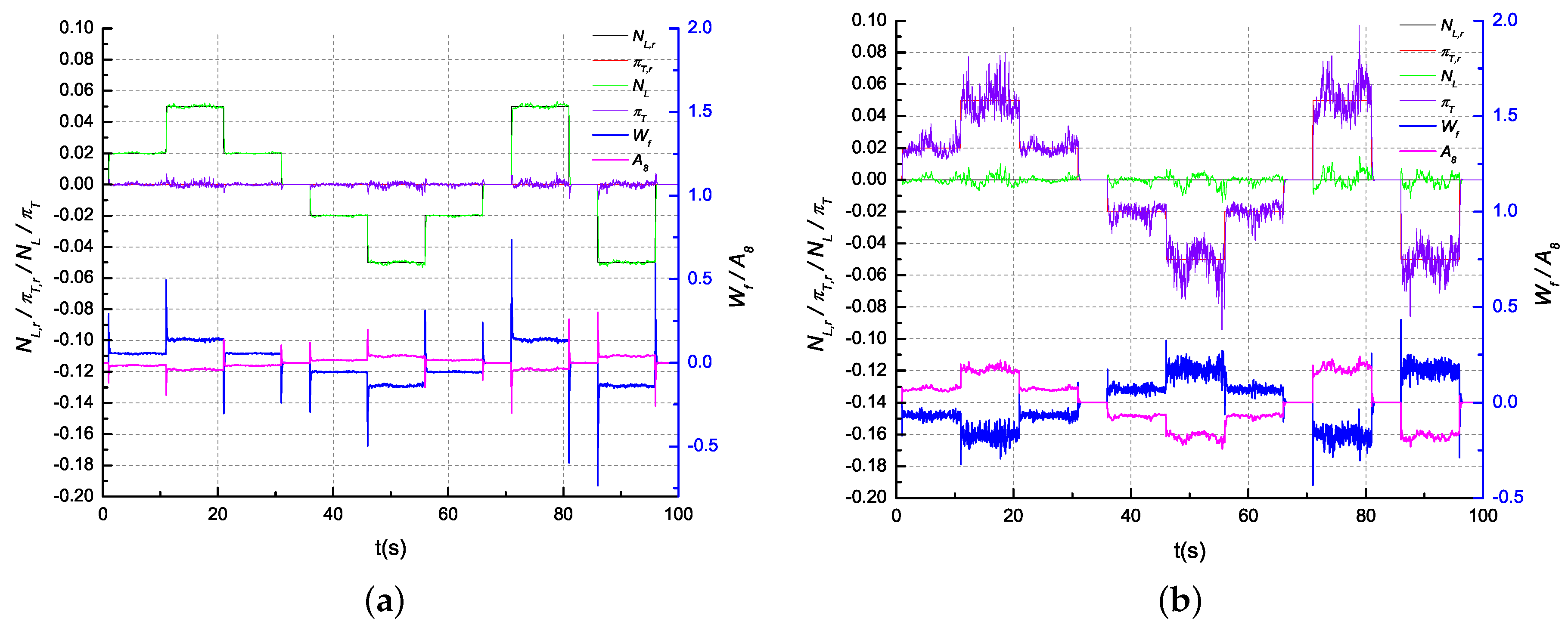
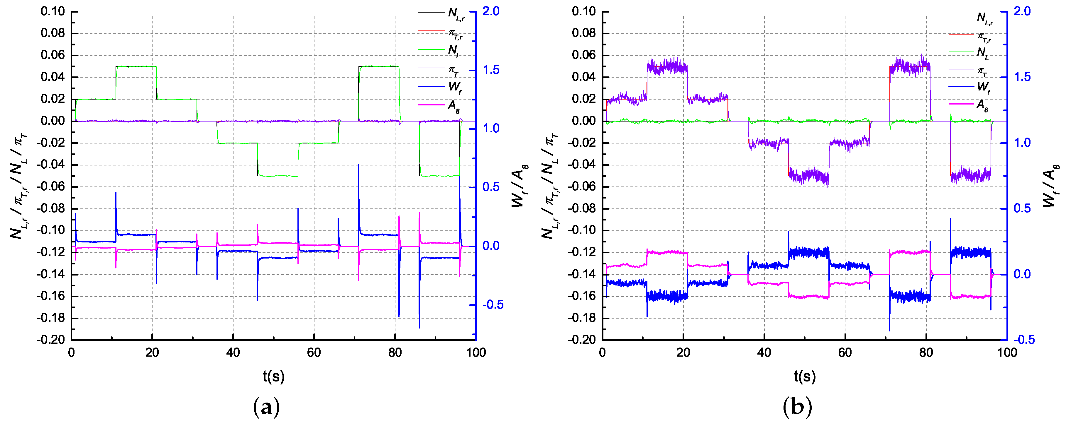
Figure 5 depicts the responses of states and control inputs during the step of and under the control. The responses curves indicate that and can track the references steps in 0.6 s and 0.3 s, respectively. The tracking errors are less than and . For , we know by (A18). Furthermore, by (A19)–(A20) and (A37), we obtain: (1) if , then ; (2) if , then . It is concluded that the tracking error bounds from the simulations’ results are less than those of the designed calculation, which indicates that the /Leitmann control achieves the desired tracking performance and has the satisfied robustness in the resistance of uncertainty and noise.
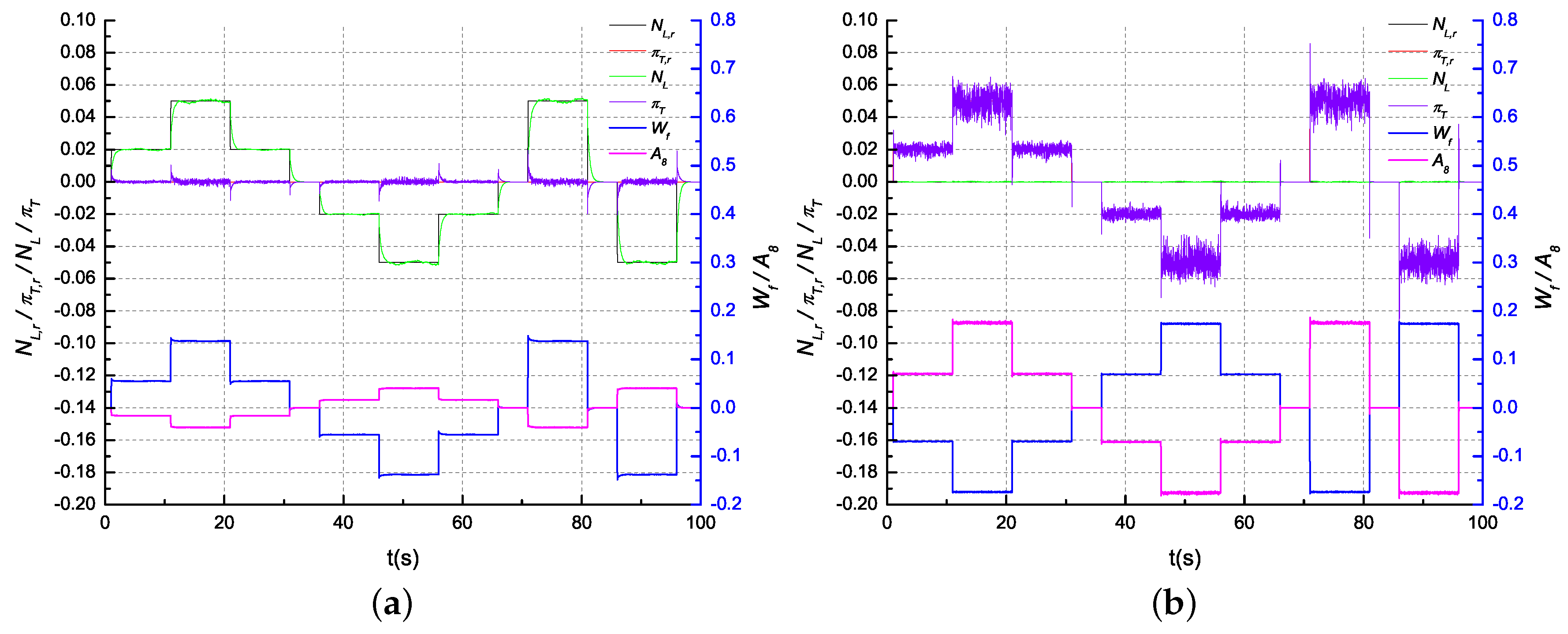
To demonstrate the ability that the control constrains the uncertainty, we conducted the same simulation procedure with only the control, and the controller gain matrix was adopted as in (38). The simulation results are shown in Figure 6. By comparison with Figure 5, the response of in Figure 6 appears as a tiny wave during steps, and the situation is much worse in the response of shown in Figure 5b. We also can see from Figure 5b that the maximal magnitude of perturbations reaches almost , and the curve waves are stronger, while in Figure 6b, this value is around .
We adopt the LQR controller (45) to conduct the same simulation procedure as that in Figure 5. The results are shown in Figure 7. By comparison with Figure 5a,b, respectively, we can find that, in Figure 7a, steps cause around perturbations of , and in Figure 7b, ’s overshoots reach around . Both of these results are greater than those in Figure 5.
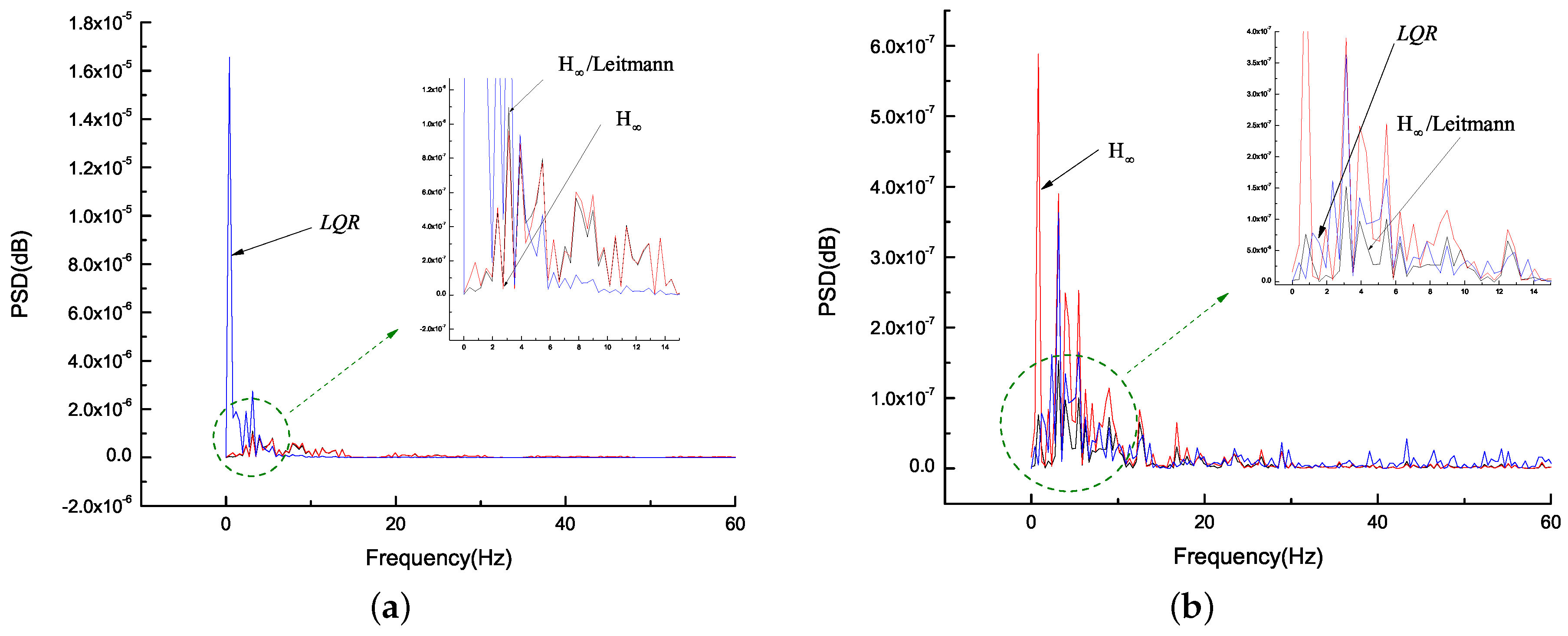
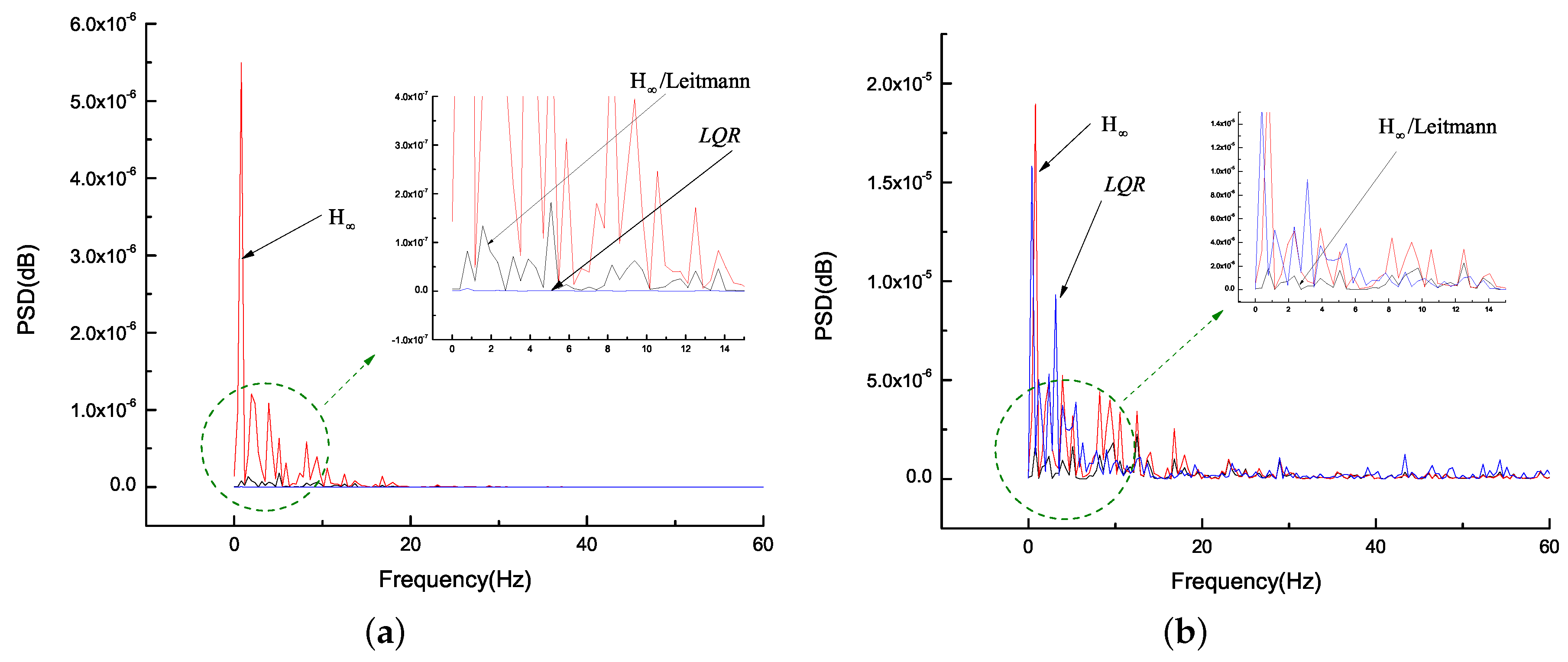
Furthermore, we analyze the power spectral densities (PSDs) of and in Figure 5, Figure 6 and Figure 7, and Figure 8 and Figure 9 show the analysis results. From Figure 8a, it is shown that during the step, the PSD peaks of under the controller (41), controller (38) and LQR controller are , and . It shows that, with respect to uncertainty and noise, the /Leitmann controller has better robustness than the other two controllers, especially in the period of [0, 20 dB]. Figure 8b shows, during the same step, the PSD of under the three controllers. The PSD peaks are, respectively, , and . It demonstrates that the /Leitmann approach has a better decoupling between and . A similar situations exist in Figure 9a,b. It can be concluded from these analysis results that no matter in the step or in step, /Leitmann controller has the best capacity for uncertainty and noise resistance and for and decoupling.
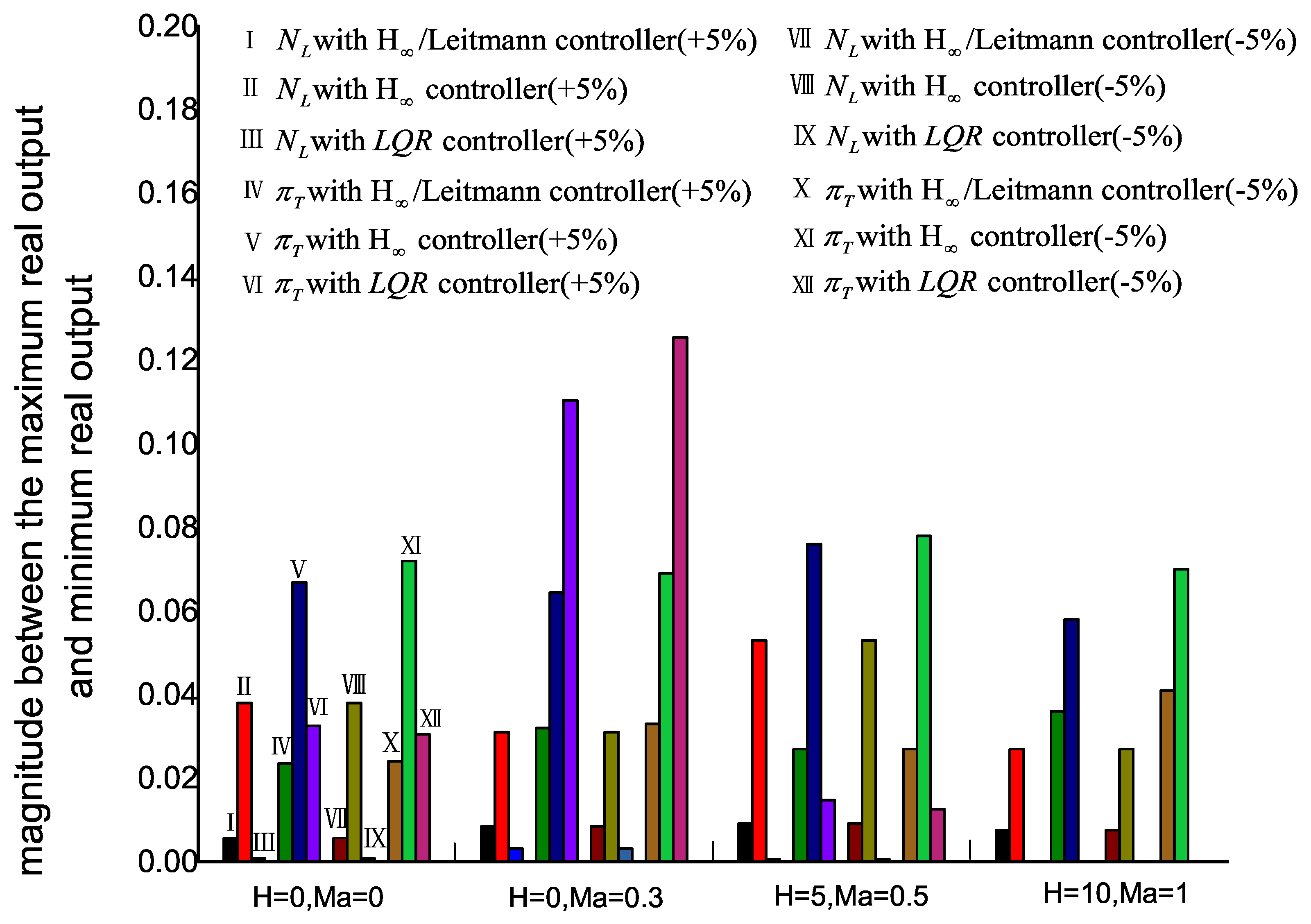
With the varying of the operation point in the flight envelope, the characteristics of the turbofan changes nonlinearly. To validate the robustness of our controller in the flight envelop, we chose three more conditions: km, ; km, ; km, ; applying the same /Leitmann controller to these three operating points and making the same simulation procedure as that at . Figure 10 shows the results of km, . For comparison, the same simulations were performed with the controller and the controller. The corresponding results are shown in Figure 11 and Figure 12, respectively. The statistics of the output extremes under all four operating conditions are listed in Table 1 and Table 2. The magnitude between the maximum and the minimum is drawn in Figure 13 and Figure 14.
Figure 10a,b indicates that, no matter during steps or steps, the /Leitmann control can guarantee the tracking performances and has a better restraining capability of the uncertainty and the noise than that of the control at all three operating points. At km, , the controlled system has a similar tracking performance to that at .
We drew Figure 13 and Figure 14 for further illustrating the data in Table 1 and Table 2. Figure 13 and Figure 14 show the following information: (1) By /Leitmann control, under all four operating conditions, the tracking errors of and are in the bounds and , respectively, which are the smallest during the state steps in the three controllers. Moreover, during the step, the disturbances in are less than 0.01. During the , the disturbances in are less than 0.0007. These indicate that in the different operating conditions, the /Leitmann control has a good capacity of decoupling. (2) By the control, at all four operating conditions, the controlled system can guarantee the tracking performance, but the maximal perturbation of and is 0.0083 and 0.0268. This shows that the perturbation deteriorates with the variety of the operating condition. (3) By the LQR control, at the parts of the operating condition, the controlled system has satisfactory performance, such as at km, and km, . However, the state behaviors of the controlled system get bad at km, and are even worse at km, where the controlled system is unstable.
5. Conclusions
To meet a high quality of tracking requirements, as well as attenuate the uncertainty and noise, of aircraft turbofans, a new tracking control design is developed in this paper. The tracking control system is modeled as three parts: the nominal system, the uncertainty and the reference model. The tracking performances, UTB and UUTB, are built. For this tracking control system, the robust control is proposed based on control and the Leitmann approach. The significance of the work is two-fold. Firstly, the control guarantees the baseline performances, namely the asymptotical stability and the noise suppression of the nominal system. Secondly, in the presence of uncertainty, the performances of UTB and UUTB are further achieved by the collaboration of the Leitmann approach and the control. The new approach is applied to design the multi-variable controller for an aircraft turbofan. The computer simulations validate that: (1) when the dynamics of the controlled system varies in the flight envelope, the new approach could guarantee the robustness of the closed-loop system and the tracking bounds of and are and ; (2) in comparison with the classical robust controls, and , the new approach shows the best performances in the resistance of uncertainty and noise. The control can realize stable robust control in all four operating points of the turbofan, but the bounds of the state responses are around 200% or even more than those of the new approach. The control can only work at the parts of the operating conditions. At these working operating conditions, the state step responses show a limited ability at reducing the influences of uncertainty and noise. The results of this paper might encourage further hardware-in-loop simulations and physical tests of the new designed controlled turbofan system.
Acknowledgments
This work was supported by (1) the National Natural Science Foundation of China (No. 51406084) and (2) the Jiangsu Province Key Laboratory of Aerospace Power System(NJ20160020).
Author Contributions
Muxuan Pan, Ye-hwa Chen and Jinquan Huang conceived the new robust control approach and the control scheme. Muxuan Pan and Kaiwen Zhang designed the new robust controller. Kaiwen Zhang built the linear model of the turbofan engine and conducted the simulation. Muxuan Pan and Kaiwen Zhang analyzed the simulation results and wrote the paper.
Conflicts of Interest
The authors declare no conflict of interest.
Appendix A
For the system (24), we choose the Lyapunov function candidate:
Here, .
For a given scalar , define . Introducing into the matrix inequality (25), it follows:
Multiply (A2) with in the right and left and yield:
By (26) and (28), (A3) can be written as:
Multiply } in the right and left of (A4), and consider (23); we have:
By adopting the Schur complement, (A5) is equivalent to:
For any , consider:
By (A6), we know:
Consider the zero initial condition,
Let T →∞,
By (A10), the transfer function of System (24) satisfies:
Appendix B
For the system (29), we choose the Lyapunov function candidate:
Here, P was decided in (28). The derivative of along any solution of (29) is given by:
As a consequence of (12), (30) and (31), it follows:
From (30) and (31), we know if ,
and if ,
Consequently, for all :
Give a positive scalar r, and let:
Define:
We now prove the uniform tracking boundedness of the system (29) by contradiction. Consider the system (29) subject to Assumptions 1–3. If , we suppose there exists a time , such that:
This suggests that there exists a , such that:
This result contradicts (A23). Hence:
and the system (29) is uniform tracking boundedness. We impose no constraint on the upper limitation of time in (A29), so it can extend to infinity, namely,
Next, we prove the uniform ultimate tracking boundedness of the controlled system (29). Suppose . Consider ; by definition of , we get:
If , then . In view of the proof of uniform tracking boundedness, we can get:
Hence:
If , we also take the contradiction to prove that . We suppose that ,
where:
As a consequence of the tracking uniform boundedness,
Finally,
References
- Ballal, D.R.; Zelina, J. Progress in aero engine technology. J. Aircr. 2004, 41, 43–50. [Google Scholar] [CrossRef]
- Lyantsev, O.D.; Breikin, T.V.; Kulikov, G.G.; Arkov, V.Y. On-line performance optimisation of aero engine control system. Automatica 2003, 39, 2115–2121. [Google Scholar] [CrossRef]
- Roquemore, W.M.; Shouse, D.; Burrus, D.; Johnson, A.; Cooper, C.; Duncan, B.; Vihinen, I. Vortex combustor concept for gas turbine engines. In Proceedings of the 39 th Aerospace Sciences Meeting and Exhibit, Reno, NV, USA, 8–11 January 2001. [Google Scholar]
- Soeder, J. F. F100 Multivariable Control Synthesis Program: Computer Implementation of the F100 Multivariable Control Algorithm; NASA: Cleveland, OH, USA, 1983; 2231.
- Pandey, S.K.; Mohanty, S.R.; Kishor, N.; Catalão, J.P. An Advanced LMI-Based-LQR Design for Load Frequency Control of an Autonomous Hybrid Generation System. In Technological Innovation for the Internet of Things; Springer: Berlin/Heidelberg, Germany, 2013; pp. 371–381. [Google Scholar]
- Pfeiffer, R.; Haraldsson, G.; Olsson, J.O.; TunestAl, P.; Johansson, R.; Johansson, B. System identification and LQG control of variable-compression HCCI engine dynamics. In Proceedings of the 2004 IEEE International Conference on Control Applications, Lund, Sweden, 2–4 September 2004; pp. 1442–1447. [Google Scholar]
- Karlsson, M.; Ekholm, K.; Strandh, P.; Johansson, R.; Tunestal, P. LQG control for minimization of emissions in a diesel engine. In Proceedings of the 2008 IEEE International Conference Control Applications, San Antonio, TX, USA, 3–5 September 2008; pp. 245–250. [Google Scholar]
- Sundararajan, N.; Joshi, S.M.; Armstrong, E.S. Attitude control system synthesis for the Hoop/Column antenna using the LQG/LTR method. Proceedings of Astrodynamics Conference, Williamsburg, VA, USA, 18–20 August 1986; pp. 469–478. [Google Scholar]
- Yuan, X.C.; Guo, Y.Q. Non-fully recovering LQG/LTR method and its application in aeroengine control. In Proceedings of the 43rd AIAA/ASME/SAE/ASEE Joint Propulsion Conference & Exhibition Re-Ston, Cincinnati, OH, USA, 8–11 July 2007; pp. 1–7. [Google Scholar]
- Härefors, M. Application of H∞ robust control to the RM12 jet engine. Control Eng. Pract. 1997, 5, 1189–1201. [Google Scholar] [CrossRef]
- Kar, I.N.; Miyakura, T.; Seto, K. Bending and torsional vibration control of a flexible plate structure using H∞-based robust control law. IEEE Trans. Control Syst. Technol. 2000, 8, 545–553. [Google Scholar] [CrossRef]
- Alikhani, H.R.; Motlagh, M.M. Aero Engine Multivariable Robust Control. TJEAS J. 2016, 5, 228–232. [Google Scholar]
- Lu, L.; Turkoglu, K. H∞ Loop-Shaping Robust Differential Thrust Control Methodology for Lateral/Directional Stability of an Aircraft with a Damaged Vertical Stabilizer. In Proceedings of the AIAA Guidance, Navigation, and Control Conference, San Diego, CA, USA, 4–8 January 2016; p. 1624. [Google Scholar]
- Qian, K.; Pang, X.; Xie, S.; He, X. Aeroengine PID multi-variable decoupling control system based on dynamic NNI. In Proceedings of the 2007 IEEE International Conference on Control and Automation, Guangzhou, China, 30 May–1 June 2007; pp. 2685–2689. [Google Scholar]
- Vesterback, J.; Bochko, V.; Ruohonen, M.; Alander, J.; Bäck, A.; Nylund, M.; Östman, F. Engine parameter outlier detection: Verification by simulating PID controllers generated by genetic algorithm. In International Symposium on Intelligent Data Analysis; Springer: Berlin/Heidelberg, Germany, 2012; pp. 404–415. [Google Scholar]
- Leitmann, G. On the efficacy of nonlinear control in uncertain linear systems. J. Dyn. Syst. Meas. Control 1981, 103, 95–102. [Google Scholar] [CrossRef]
- Leitmann, G. On one approach to the control of uncertain systems. J. Dyn. Syst. Meas. Control 1993, 115, 373–380. [Google Scholar] [CrossRef]
- Corless, M. Control of uncertain nonlinear systems. J. Dyn. Syst. Meas. Control 1993, 115, 362–372. [Google Scholar] [CrossRef]
- Xiong, Z.K.; Leitmann, G.; Garofalo, F. Robustness of uncertain dynamical systems with delay without matching assumptions. IFAC Proc. Ser. 1989, 1, 269–273. [Google Scholar]
- Yu, Y. On stabilizing uncertain linear delay systems. J. Optim. Theory Appl. 1983, 41, 503–508. [Google Scholar] [CrossRef]
- Chen, Y.H.; Leitmann, G.; Kai, X.Z. Robust control design for interconnected systems with time-varying uncertainties. Int. J. Control 1991, 54, 1119–1142. [Google Scholar] [CrossRef]
- Hu, Y.; Ng, A. Active robust vibration control of flexible structures. J. Sound Vib. 2005, 288, 43–56. [Google Scholar] [CrossRef]
- Zhang, X.; Zhao, J. An algorithm of uniform ultimate boundedness for a class of switched linear systems. Int. J. Control 2002, 1, 166–170. [Google Scholar] [CrossRef]
- Aleksandrov, A.Y.; Chen, Y.; Platonov, A.V.; Zhang, L. Stability analysis and design of uniform ultimate boundedness control for a class of nonlinear switched systems. J. Differ. Equ. Appl. 2009, 18, 944–949. [Google Scholar]
- Burkan, R. Modelling of Bound Estimation Laws and Robust Controllers for Robot Manipulators Using Functions and Integration Techniques. J. Intell. Robot. Syst. 2010, 60, 365–394. [Google Scholar] [CrossRef]
- Lu, X.Y.; Spurgeon, S.K. Robust sliding mode control of uncertain nonlinear systems. Syst. Control Lett. 1997, 32, 75–90. [Google Scholar] [CrossRef]
- Chen, Y.H. A new approach to the control design of fuzzy dynamical systems. J. Dyn. Syst. Meas. Control 2011, 133, 061019. [Google Scholar] [CrossRef]
- Huang, J.; Chen, Y.H.; Cheng, A. Robust Control for Fuzzy Dynamical Systems: Uniform Ultimate Boundedness and Optimality. IEEE Trans. Fuzzy Syst. 2012, 20, 1022–1031. [Google Scholar] [CrossRef]
- Xiong, D.; Chen, Y.H.; Zhao, H. Optimal robust decentralized control design for fuzzy complex systems. J. Intell. Fuzzy Syst. 2014, 26, 211–222. [Google Scholar]
- Zhang, R.; Pan, M.; Huang, J. Network-based guaranteed cost tracking control for aero-engine. In Proceedings of the Asia-Pacific International Symposium on Aerospace Technology (APISAT 2015), Canberra, Australia, 25–27 November 2015; pp. 292–301. [Google Scholar]
- Kulikov, G.G.; Thompson, H.A. (Eds.) Dynamic Modelling of Gas Turbines: Identification, Simulation, Condition Monitoring and Optimal Control; Springer Science & Business Media: London, UK, 2004; pp. 89–116. [Google Scholar]
Figure 1.
Structure of a turbofan.
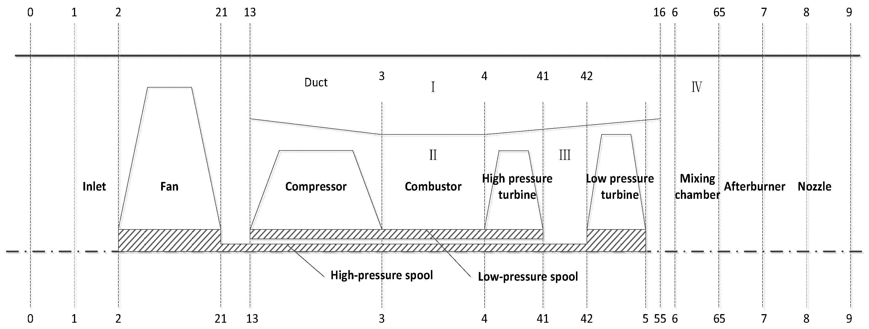
Figure 2.
Scheme of the turbofan tracking control.

Figure 3.
Noise histories, .

Figure 4.
Uncertain parameter history, .

Figure 5.
Histories of states and controls under the /Leitmann control at . (a) Responses of states and controls during steps; (b) responses of states and controls during steps.
Figure 5.
Histories of states and controls under the /Leitmann control at . (a) Responses of states and controls during steps; (b) responses of states and controls during steps.
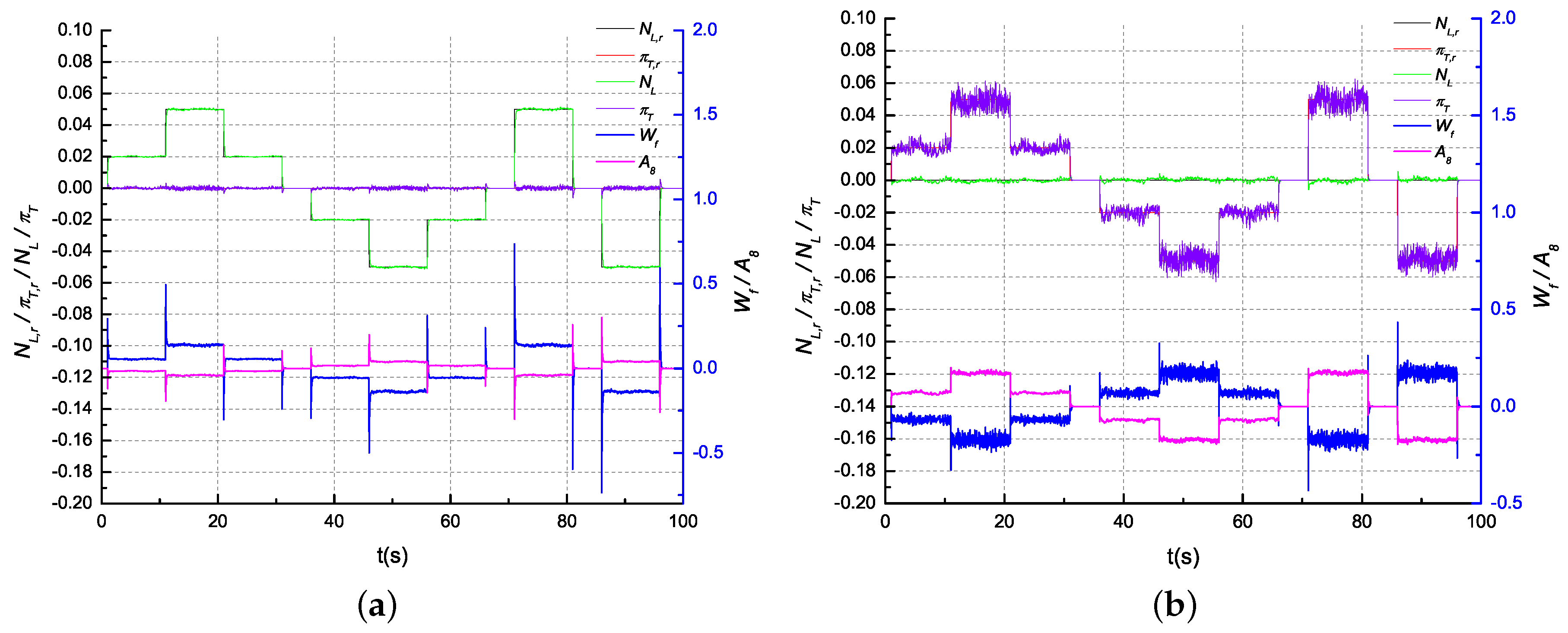
Figure 6.
Histories of states and controls under the control at . (a) Responses of states and controls during steps; (b) responses of states and controls during steps.
Figure 6.
Histories of states and controls under the control at . (a) Responses of states and controls during steps; (b) responses of states and controls during steps.

Figure 7.
Histories of states and controls under the linear quadratic regulator (LQR) control at , . (a) Responses of states and controls during steps; (b) responses of states and controls during steps.
Figure 7.
Histories of states and controls under the linear quadratic regulator (LQR) control at , . (a) Responses of states and controls during steps; (b) responses of states and controls during steps.

Figure 8.
Power spectral densities (PSDs) of the state responses during the steps and under the three different controls. (a) PSDs of ; (b) PSDs of .
Figure 8.
Power spectral densities (PSDs) of the state responses during the steps and under the three different controls. (a) PSDs of ; (b) PSDs of .

Figure 9.
PSDs of the state responses during the steps and under the different controls. (a) PSDs of ; (b) PSDs of .
Figure 9.
PSDs of the state responses during the steps and under the different controls. (a) PSDs of ; (b) PSDs of .

Figure 10.
States histories under the /Leitmann control at km, . (a) State and control response during steps; (b) state response during steps.
Figure 10.
States histories under the /Leitmann control at km, . (a) State and control response during steps; (b) state response during steps.

Figure 11.
States histories under the control at km, . (a) State and control response during steps; (b) state response during steps.
Figure 11.
States histories under the control at km, . (a) State and control response during steps; (b) state response during steps.
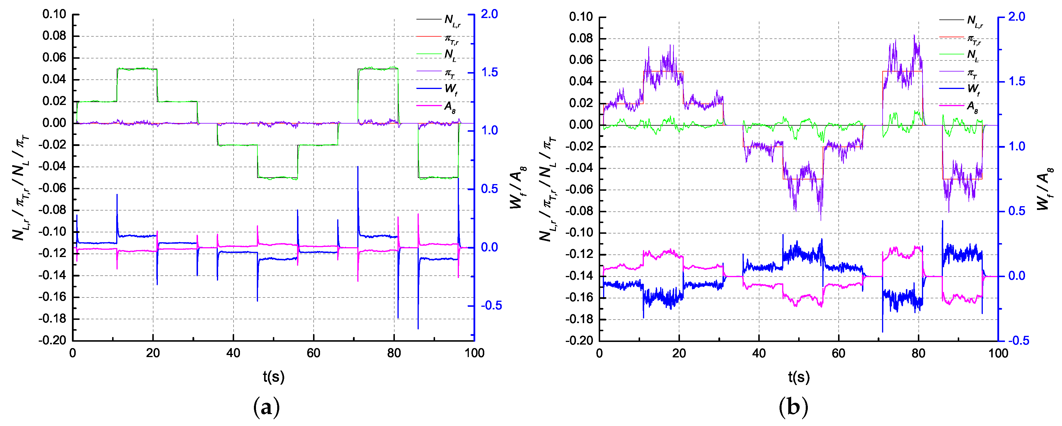
Figure 12.
States histories under the LQR control at km, . (a) State and control response during steps; (b) state response during steps.
Figure 12.
States histories under the LQR control at km, . (a) State and control response during steps; (b) state response during steps.
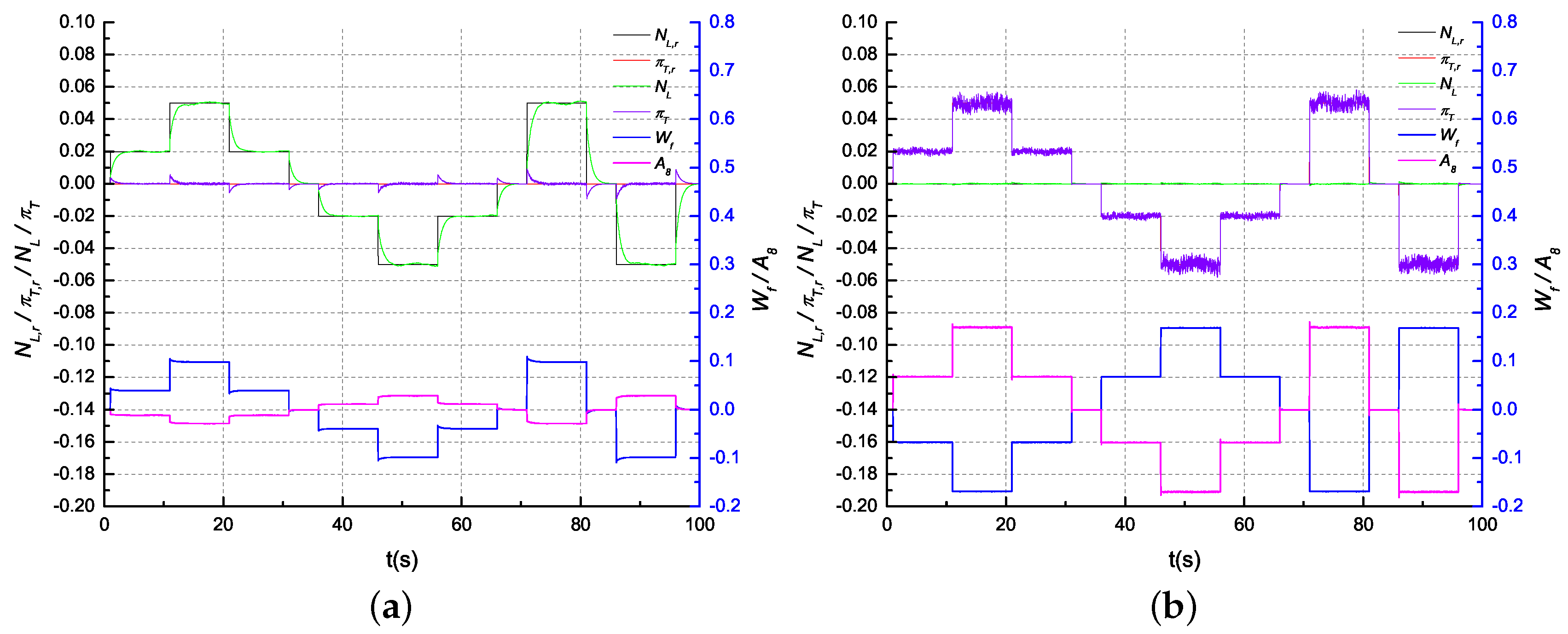
Figure 13.
Magnitudes in different conditions during steps.
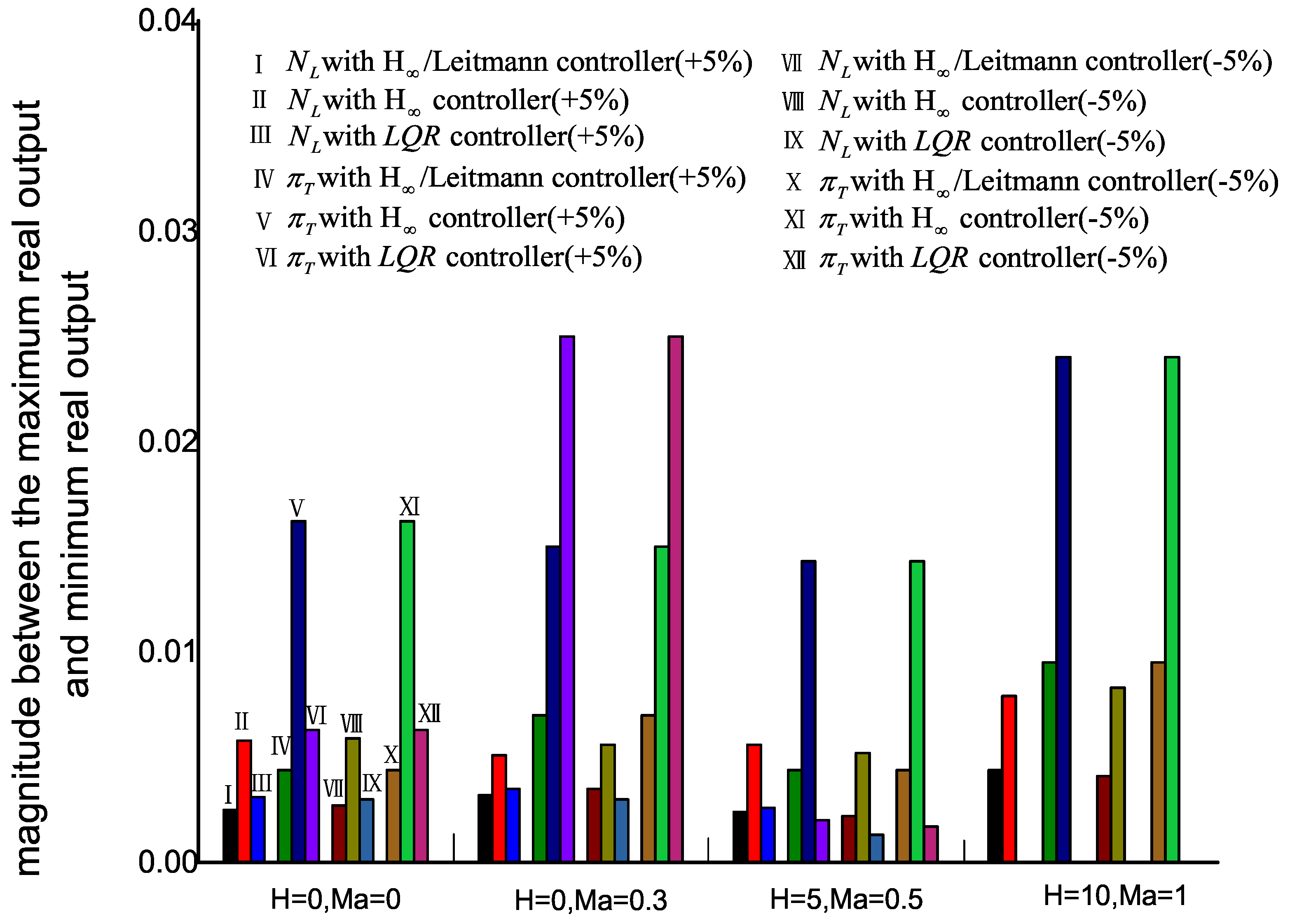
Figure 14.
Magnitudes in different conditions during steps.

Table 1.
extremes at different conditions. NaN—Not a Number.
| Operating Condition | Step | (Min/Max) | ||
|---|---|---|---|---|
| /Leitmann | LQR | |||
| km | (5%) | 0.0512/0.0487 | 0.0536/0.0478 | 0.0516/0.0485 |
| (−5%) | −0.0488/−0.0515 | −0.0481/−0.0540 | −0.0487/−0.0517 | |
| (5%) | 0.0026/−0.0030 | 0.0180/−0.0198 | 0.0004/−0.0004 | |
| (−5%) | 0.0024/−0.0031 | 0.0178/−0.0200 | 0.0004/−0.0004 | |
| km | (5%) | 0.0517/0.0485 | 0.0531/0.0480 | 0.0518/0.0483 |
| (−5%) | −0.0485/−0.0520 | −0.0481/−0.0537 | −0.0484/−0.0514 | |
| (5%) | 0.0039/−0.0043 | 0.0140/−0.0168 | 0.0016/−0.0017 | |
| (−5%) | 0.0037/−0.0045 | 0.0138/−0.0170 | 0.0015/−0.0018 | |
| km | (5%) | 0.0513/0.0489 | 0.0538/0.0482 | 0.0515/0.0489 |
| (−5%) | −0.0491/−0.0513 | −0.0485/−0.0537 | −0.0489/−0.0502 | |
| (5%) | 0.0042/−0.0048 | 0.0270/−0.0258 | 0.0002/−0.0004 | |
| (−5%) | 0.0040/−0.0050 | 0.0269/−0.0260 | 0.0002/−0.0004 | |
| km | (5%) | 0.0523/0.0479 | 0.0548/0.0469 | −NaN/−NaN |
| (−5%) | −0.0482/−0.0523 | −0.0472/−0.0555 | −NaN/−NaN | |
| (5%) | 0.0035/−0.0038 | 0.0125/−0.0143 | −NaN/−NaN | |
| (−5%) | 0.0033/−0.0040 | 0.0123/−0.0145 | −NaN/−NaN | |
Table 2.
The output extremes at different conditions. (NaN—Not a Number)
| Operating Condition | Step | (Min/Max) | ||
|---|---|---|---|---|
| /Leitmann | LQR | |||
| km | (5%) | 0.0021/−0.0020 | 0.0076/−0.0083 | 0.0031/−0.0032 |
| (−5%) | 0.0020/−0.0023 | 0.0073/−0.0086 | 0.0031/−0.0033 | |
| (5%) | 0.0617/0.0381 | 0.0980/0.0311 | 0.0640/0.0315 | |
| (−5%) | −0.0380/−0.0620 | −0.0320/−0.1040 | −0.0340/−0.0645 | |
| km | (5%) | 0.0035/−0.0033 | 0.0070/−0.0078 | 0.0125/−0.0125 |
| (−5%) | 0.0032/−0.0035 | 0.0068/−0.0080 | 0.0125/−0.0125 | |
| (5%) | 0.0670/0.0350 | 0.0962/0.0318 | 0.0955/−0.0149 | |
| (−5%) | −0.0350/−0.0680 | −0.0330/−0.1020 | 0.0140/−0.1115 | |
| km | (5%) | 0.0019/−0.0023 | 0.0070/−0.0071 | 0.0010/−0.0010 |
| (−5%) | 0.0018/−0.0025 | 0.0069/−0.0073 | 0.0008/−0.0009 | |
| (5%) | 0.0640/0.0370 | 0.1050/0.0290 | 0.0582/0.0434 | |
| (−5%) | −0.0380/−0.0650 | −0.0310/−0.1090 | −0.0435/−0.0561 | |
| km | (5%) | 0.0045/−0.0048 | 0.0100/−0.0139 | −NaN/−NaN |
| (−5%) | 0.0044/−0.0050 | 0.0098/−0.0140 | −NaN/−NaN | |
| (5%) | 0.0670/0.0310 | 0.0870/0.0290 | −NaN/−NaN | |
| (−5%) | −0.0280/−0.0690 | −0.0310/−0.1010 | −NaN/−NaN | |
© 2017 by the authors. Licensee MDPI, Basel, Switzerland. This article is an open access article distributed under the terms and conditions of the Creative Commons Attribution (CC BY) license (http://creativecommons.org/licenses/by/4.0/).
Share and Cite
MDPI and ACS Style
Pan, M.; Zhang, K.; Chen, Y.-H.; Huang, J. A New Robust Tracking Control Design for Turbofan Engines: H∞/Leitmann Approach. Appl. Sci. 2017, 7, 439. https://doi.org/10.3390/app7050439
AMA Style
Pan M, Zhang K, Chen Y-H, Huang J. A New Robust Tracking Control Design for Turbofan Engines: H∞/Leitmann Approach. Applied Sciences. 2017; 7(5):439. https://doi.org/10.3390/app7050439
Chicago/Turabian StylePan, Muxuan, Kaiwen Zhang, Ye-Hwa Chen, and Jinquan Huang. 2017. "A New Robust Tracking Control Design for Turbofan Engines: H∞/Leitmann Approach" Applied Sciences 7, no. 5: 439. https://doi.org/10.3390/app7050439
Note that from the first issue of 2016, this journal uses article numbers instead of page numbers. See further details here.