
A Multi-View Stereo Algorithm Based on Homogeneous Direct Spatial Expansion with Improved Reconstruction Accuracy and Completeness

1
College of Physical Science and Technology, Central China Normal University, Wuhan 430079, China
2
School of Electronic Information and Electrical Engineering, Xiangnan University, Chenzhou 423000, China
*
Author to whom correspondence should be addressed.
Appl. Sci. 2017, 7(5), 446; https://doi.org/10.3390/app7050446
Submission received: 12 February 2017
/
Revised: 14 April 2017
/
Accepted: 21 April 2017
/
Published: 29 April 2017
Abstract
:Reconstruction of 3D structures from multiple 2D images has wide applications in such fields as computer vision, cultural heritage preservation, etc. This paper presents a novel multi-view stereo algorithm based on homogeneous direct spatial expansion (MVS-HDSE) with high reconstruction accuracy and completeness. It adopts many unique measures in each step of reconstruction, including initial seed point extraction using the DAISY descriptor to increase the number of initial sparse seed points, homogeneous direct spatial expansion to enhance efficiency, initial value modification via a conditional-double-surface-fitting method before optimization and adaptive consistency filtering after optimization to ensure high accuracy, processing using a multi-level image pyramid to further improve completeness and efficiency, etc. As demonstrated by experiments, owing to above measures the proposed algorithm attained much improved reconstruction completeness and accuracy.
1. Introduction
3D reconstruction software, which takes in digital photos or videos and outputs 3D models, has been the goal of many researchers for past decades. When such software becomes available, 3D modeling might become a routine practice even for ordinary people using digital devices like digital cameras and smart phones, rather than a privilege enjoyed by those with professional equipment like laser-based scanners, structure light scanners, etc., not to mention the building of 3D models at city scale, where photo-based methods seem the most suitable choice. It’s possible to produce long list of existing research aimed at this ultimate goal. Table 1 provides a short list of such work, identified by their technical features. For more work in this field, we refer readers to the review articles presented in [1,2,3].
Multi-view 3D reconstruction can be traced back to binocular stereopsis based on window matching and triangulation. However, this window-based matching produces reliable results only for texture-rich regions. When it was extended to multi-view situations, it was adapted to feature-matching and triangulation, giving rise to Structure From Motion (SFM) [4], which is widely used today for extraction of sparse seed points and camera calibration. To reconstruct the remaining regions and cope with difficulties like occlusion, non-Lambert illumination, photo noise, etc., many kinds of algorithm have been developed. They could be roughly classified into volume-based algorithms, depth-map fusion algorithms and feature-expansion algorithms.
Volume-based algorithms represent the space occupied by an object with voxels or a surrounding surface. Take the algorithm of Seitz et al. [5] in Table 1, for example, which discretizes a 3D scene into voxels and assigns colors to them, so as to achieve consistency with all the input images. To solve the occlusion problem, it decomposes the 3D scene into layers and sweeps them outward from the camera volume (the convex hull formed by the camera centers) in a single pass, with the constraint that no scene point is contained within the camera volume. This constraint on camera position was avoided by using a multi-sweep method, as suggested by Kutulakos et al. [6]. The multi-sweep approach takes place in six principle directions. For each voxel, the activated cameras are located on one side of the sweep plane. Vogiatzis et al. [8] explored another approach based on the idea that all potential causes of mismatches, like occlusion, image noise, lack of texture, or highlights, can be uniformly treated as outliers in the matching process. Matching is then seen as a process of robust model fitting to data that contains outliers. In [8], the model was represented using a cost functional solved via global optimization using Graph-cuts. In [7] the cost functional took into consideration the non-Lambertian appearance of the scene, and was minimized using the level set method. Volume-based algorithms reconstruct the entire object completely. However, many of them need a good initial estimation of the object to avoid converging into local minima. Their accuracy is usually limited by voxel size. As the size of the voxels becomes smaller, the number of voxels increases cubically, implying ahuge consumption of CPU time and memory. So volume-based algorithms have been demonstrated in the reconstruction of relatively small objects, as shown in Table 1.
Depth-map fusion algorithms, in principle, are capable of dealing with both small objects and large scenes. Many of them make use of a two-stage approach that estimates a depth map for each image and then merges all the depth maps to extract a final surface [17,18]. Early multi-view depth-map fusion algorithms were simple extensions of window-based binocular stereo matchers, which often contained a large amount of noise. Many more advanced depth-map fusion algorithms were subsequently developed utilizing powerful optimization methods like graph cut [9], expectation maximization [19], sequential tree-reweighted message passing [11], etc. These global optimization methods were either used in extraction of each depth map or in the final merging of all the depth maps. Goesele et al. [10] and Tola et al. [12] went back to find the depth locally. Goesele simply discarded the bad matches in texture-weak regions to avoid noise. Tola went much further by introducing a DAISY descriptor [20]. The DAISY descriptor outperforms NCC, since it contains much more information than plain intensity distributions in small windows. For the selection of the best points instantiated from several different image pairs [12], preference was given to the points obtained by larger focal length, larger baseline and closer camera. To the best of our knowledge, Tola attained the highest reconstruction accuracy [1,2]. More importantly, this accuracy was obtained on large-scale, high-resolution data sets with high efficiency, which is of great significance, since millions of high-resolution photos are produced everyday around the world. City-scale [21] and civil-infrastructure [22,23,24] reconstructions have been receiving a lot of attention recently.
Feature expansion algorithms provide another efficient way of producing dense 3D clouds. The basic idea of feature expansion or region growing was demonstrated as early as 1989 by Otto et al. [13] for the processing of satellite photos. They started from a few seed points and performed area-based matching using Gruen’s adaptive least-squares correlation algorithm [25]. Following successful matching, the distortion parameters were applied to nearby pixels as initial parameters, and the growing process was repeated for the remaining regions. Habbecke et al. [15] provided a surface-growing approach in the form of disk expansion based on the discrepancy induced by the sum of squared differences (SSD). New disks were expanded by user-specified fractions of the parent disk’s minimal radius. Goesele et al. [14] developed a feature expansion algorithm to find high-quality depth maps. They suppressed outliers through a combination of intelligent image selection at per-view and per-pixel levels, and a sequential expansion strategy based on a priority queue. Their algorithm was capable of addressing the extreme changes in lighting, scale, clutter, and other effects in large online-community photo collections. Furukawa et al. [16] arrived at a patch-based feature expansion algorithm, Patch-based Multi-View Stereopsis (PMVS), which consisted of three key steps: match, expand, and filter. In the first step, sparse features were matched using Harris and difference-of-Gaussians operators. The last two steps iterate n times to spread the initial matches to nearby pixels and obtain a dense set of patches. From Otto et al. to Furukawa et al., in addition to the improvements in performance, the three key steps in the feature expansion algorithm framework became increasingly clear. The last step—the filtering of outliers—was not fully implemented until Furukawa et al. As a result, [14,15] had to adopt greedy or best-first sequential strategies, as shown in Table 1, to suppress outliers. With the filtering of outliers based on visibility and weak neighborhood regulation, [16] was able to expand all the patches with the same priority. PMVS is now regarded as a state-of-the-art MVS algorithm. Nevertheless, there is still a lot of room for improvement in the framework and in the key steps of the feature expansion algorithm. For example, the assignment of the next expanding point still relies on a reference image, i.e., the assignment is conducted in a local coordinate system, rather than occurring directly in a fixed-world coordinate system.
This paper presents a novel MVS algorithm based on homogeneous direct spatial expansion (MVS-HDSE). It extends the framework of the feature expansion algorithm by introducing an additional step for initial value modification utilizing already-expanded neighbor points. It also makes important improvements to existing steps in order to attain high accuracy and completeness while maintaining high efficiency. Briefly, the proposed algorithm adopts many unique measures, including:
- Initial seed point extraction by the DAISY descriptor: in the seed point extraction step, the high-performance DAISY descriptor was introduced to increase the number and accuracy of seed points. Like Multi-View Reconstruction Environment (MVE) systems [26] and Visual Structure From Motion (VSFM) systems [27], the proposed algorithm can also get initial sparse seed points via SFM [4], which first detects Scale-Invariant Feature Transform (SIFT) [28] feature points in images and then matches the points between pairs of images. Seed points result from successfully-matched points following triangulation principles. However, the accuracy and number of seed points might reduce greatly due to mismatches or match failure. When the high-performance DAISY descriptor is used, the number of initial seed points might be increased multiple times, which is very helpful for reconstruction completeness and efficiency. This is because feature matching is now replaced by the DAISY descriptor’s similarity searching. The former is conducted between limited pairs of existing feature points, whereas the latter is performed along epipolar lines.
- Homogeneous direct spatial expansion: in the expansion step, all 3D seed points are given with the same priority, i.e., every seed point is simultaneously expanded to nearby 3D points. This strategy is especially suitable for parallel computation, since it is neither necessary to keep a seed priority queue for sequential growth [14], nor to grow a new seed point until it cannot grow anymore [15]. Instead, every seed point is directly expanded in 3D space with a small step along its tangent plane, and the world coordinates of the expanded 3D points are recorded directly. In other words, it does not rely on images to find the initial positions of expanded points before optimization [16]. Furthermore, it is not necessary to always update the record in all images which pixels have been optimized during optimization [16], or to merge all the depth maps estimated from a number of images after optimization [10,11]. The expanding process ends automatically when a sufficient density of 3D points is achieved.
- Conditional initial value modification: in the initial value modification step, modification is conducted when certain conditions are met. In theory, each point can be reconstructed independently via optimization, regardless of whether or not other points have been reconstructed. In reality, the initial position and normal of an expanding point are provided by adjacent seed points. If the initial values are far away from the true values, the optimization process might fail or result in a local minimum with low accuracy. So, it is important to modify the initial values to make them as close to the true values as possible. To do this, the proposed algorithm provides a so-called conditional-double-surface-fitting method. It is conditional because the fitted surface is only able to approximate the local variation of nearby real surfaces on the condition that the neighbor points of the expanding point are dense enough and centered around it. The surface fitting is conducted twice, since the second fitting becomes closer to the real surface after excluding those points with large residual errors in the first fitting. Then the point is projected back onto the fitted surface and the position and normal of the foot will be used as new initial values.
- Adaptive consistency filtering: in the filtering step, adaptive consistency filtering is conducted. Points within a small area of an object’s surface are usually consistent. If one point is inconsistent with its neighbor points, it might be an outlier. We check the consistency of every point with regard to three aspects: smoothness, depth and normal. However, as will be explained latter, factors such as the real object’s surface curvature, neighbor point density, and occlusion might greatly influence the filtering process and even lead to wrong results. So, at first, a decision needs to be made for each point as to whether to carry out filtering and, if so, the thresholds for filtering are then adaptively adjusted.
- Processing on multi-level image pyramid: in both the seed point extraction step and the expansion step, the algorithm is performed on a multi-level image pyramid. As a result, not only is the computation time reduced due to the small image size, also the number of both initial seed points and the successfully expanded points is increased considerably. Some points, which fail to expand on low-level images, may succeed on high-level images, resulting in much higher reconstruction completeness.
As can be seen in the later experiments, with the help of the above measures, our algorithm provides both high reconstruction accuracy and completeness.
The rest of the paper is organized as follows. Section 2 presents the workflow of the proposed algorithm. Then it elaborates on the four key steps of the proposed algorithm. Section 3 provides the experimental results and a comparison with other algorithms. Finally, Section 4 gives a short conclusion.
2. The Algorithm
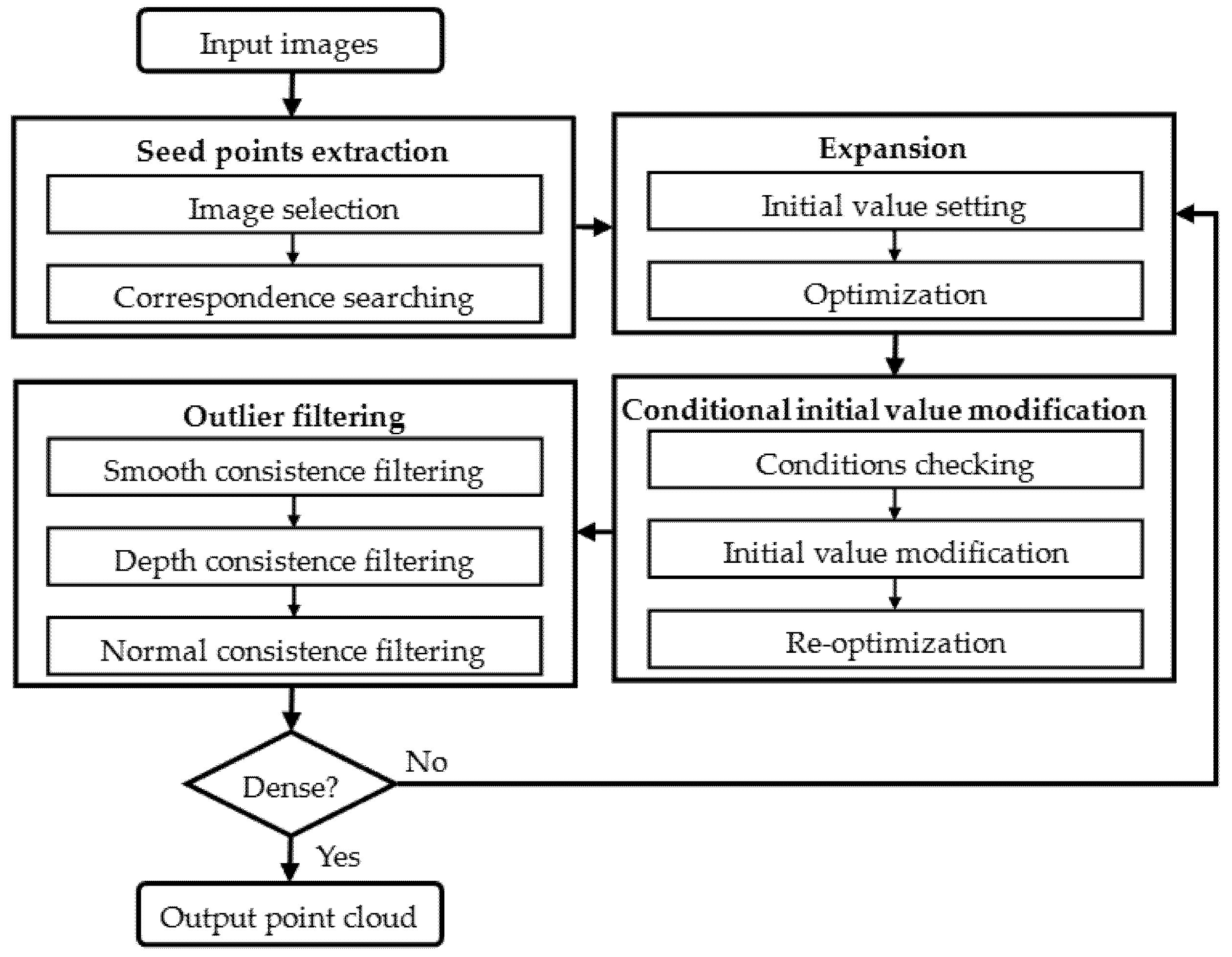
As shown in Figure 1, the proposed algorithm contains four key steps, namely seed point extraction, expansion, conditional initial value modification and outlier filtering. Firstly, sparse initial seed points are extracted from input images through a process of image selection, followed by a correspondence-search along epipolar lines; Secondly, new points are expanded on the basis of the initial positions and normals set from the seed points, and optimized for a potential increase in accuracy; Thirdly, the expanded points are modified and re-optimized on the condition that their neighbor points are sufficiently dense and centered on them. Note that once a point has been successfully modified and re-optimized, it will not be modified again; Fourthly, the outliers are deleted via consistency filtering with regard to smoothness, depth and normal. The successfully-expanded points are then used as new seeds and the last three key steps loop again and again until the final 3D point cloud becomes dense enough. More detailed descriptions are as follows.
2.1. Sparse Seed Point Extraction
Tola [12] successfully used the high-performance DAISY descriptor in a depth-map fusion algorithm. Here we try to use the DAISY descriptor in our feature expansion algorithm to extract initially sparse seed points. When feature points in a reference image are described by the DAISY descriptors, their correspondences in another image can be searched along epipolar lines. However, several peaks might be encountered in the search, and the maximum peak does not always produce the right correspondence [11]. To solve this ambiguity, the proposed algorithm searches the correspondences of one feature point in several images. Only if all correspondences are successfully found—in other words, the feature point and all its correspondences are related to a single 3D point—is the 3D point regarded as a potential seed point. The detailed process is as follows.
Firstly, each image is selected in turn as a reference image. For each reference image, at least three auxiliary images around it are selected. The parallax between any two selected images (including reference image) should be in the proper range; otherwise, matching accuracy might be reduced due to too small a parallax, and matching might even fail due to too few common regions caused by a large parallax. To ensure proper selection, scores for all candidate images can be calculated by Equation (1), and the image with highest score selected.
In Equation (1), si is the score of ith image, A is the set of all selected images (including the reference image). In our experiment, u = 15. θi,j is the angle between the optical axis of the ith camera and the jth camera. Usually, Ci = Ci,j = 1. If the ith and the jth cameras are on the same side of the camera for the reference image, Ci,j = 0.5. If the ith camera is far away from the camera for the reference image, Ci = 0.5. σ1 is defined as follows:
Secondly, correspondences for one feature point are searched in the selected images. For every feature point d in the reference image, the epiploar line l in an auxiliary image can be calculated by l = F × d, where the fundamental matrix F can be determined by at least 7 or more known matched feature points, since it contains a degree of freedom (DOF) of 7 DOF. Once enough matched feature points have been found, F can be computed using a random sample consensus (RANSAC) algorithm [29]. Then the correspondence of point d is searched at one pixel intervals along l based on the angles between DAISY descriptors. The angles are sorted in ascending order, with smaller angles indicating higher similarity. If the similarity at one point is obviously larger than that at other points as required by Expression (3) in all auxiliary images, a candidate 3D seed point can be calculated using triangulation principles and the Single Value Decomposition (SVD) method. To ensure that the found correspondences and the feature point d are related to a single 3D point, the mean reprojection error of a candidate 3D seed point in the reference and auxiliary images is calculated. A candidate 3D point becomes a true 3D seed point if its mean reprojection error is less than a threshold therr.
In Expression (3), r should be smaller than one. θi is the angle between DAISY descriptors of the feature point d and its candidate correspondences.
Since seed point extraction is performed on a multi-level image pyramid, different levels should have different thresholds therr. In our experiments for the first three levels in the image pyramid, therr = 1, 0.5 and 0.25 pixels, and r = 0.9, 0.8 and 0.7, respectively. This is because higher-level images have lower resolutions, so the threshold values become gradually stricter. Once a feature point is successfully matched, it is marked in the reference and auxiliary images to avoid repeated matching.
Finally, the normal of sparse seed points is estimated by a so-called conditional-double-surface-fitting method. This relies on the fact that the local object surface around a 3D seed point can be represented by a quadratic surface fitted over its neighboring seed points. Therefore, the normal of a 3D seed point can be estimated from the normal of the fitted surface. This works well on the condition that the surrounding seed points are sufficiently dense, and the 3D seed point is not far from the center of the surrounding points. Details of the conditional-double-surface-fitting method will be discussed a little later in Section 2.3. If the above conditions are not satisfied for a 3D seed point, its normal will simply be set as the line from itself through the optical center of the reference image.
2.2. Expansion
2.2.1. Homogeneous Direct Spatial Expansion
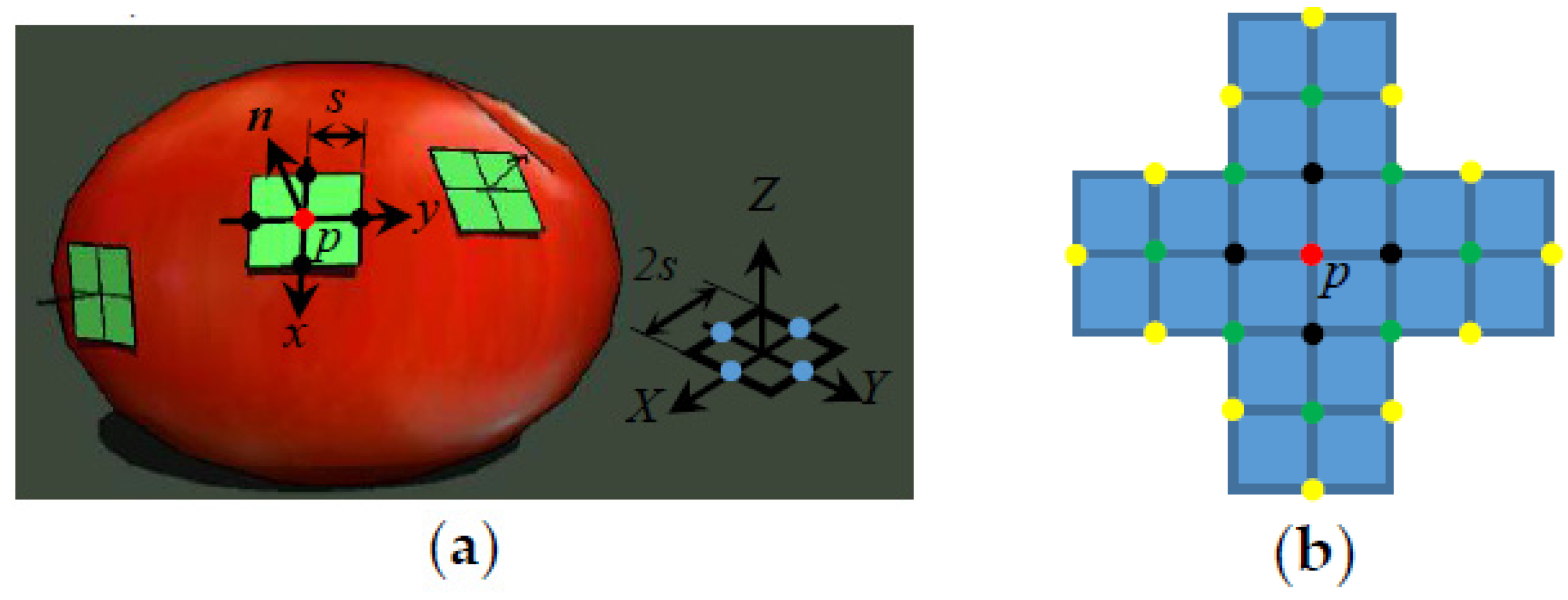
When the initial sparse seed points are extracted, they will be expanded simultaneously with a predefined small step s to nearby 3D points along two perpendicular directions, as illustrated in Figure 2. Each seed, taking the red point p in Figure 2a as an example, is expanded directly in 3D space along its tangent plane to four (black) points for later optimization. After the first iteration of expansion, the newly expanded (black) points are used as new seed points and expanded in a similar way to nearby (green) points in Figure 2b. This process repeats until the density of the 3D points is sufficient. To avoid overlap, any point that appears close to an existing point will be deleted either before or after optimization, which ensures that the final points are distributed evenly and with proper density.
The initial normal of a newly-expanded point is set the same as that of the seed point, whereas its initial world coordinate is calculated as follows. As shown in Figure 2a, first a square with a side length of 2s is drawn on the XY plane of the world coordinate system, with the centers of the four sides (blue points) placed symmetrically on the X- and Y-axis, respectively. The world coordinates of the four blue points are denoted as B. Next, the square is moved until its center coincides with point p and its normal (Z-axis positive direction) coincides with the normal of point p. The corresponding rotation matrix R can then be computed using the method in [30]. Then the new positions of the centers of the four sides (now marked black) of the square represent the initial positions of the four expanding points. Their world coordinates E can be computed by
where px, py, pz are the world coordinates of point p.
2.2.2. Optimization
As the initial position and normal are not accurate, iterative optimization based on photo-consistency is conducted to get the final accurate position and normal. Yet before the iterative optimization, a reference image and some auxiliary images need to be selected for each expanding point. For image selection, we mainly follow the methods in [14]. What we emphasize here is that only the best reference image is selected, which poses a view direction (i.e., one leading from the point to the optical center) as close as possible to the normal of the point and at a relatively shorter view distance as well. This is because only such an image can provide a relatively high resolution and relatively complete information of the region around the expanding point. After the selection of a reference image R, several auxiliary images around it are selected, which provide view direction changes usually from 15 to 40 degrees. The former is selected to guarantee the highest possible reconstruction accuracy of the position of the expanding point on its tangent plane, whereas the later mainly serve to determine its position along its normal. After each iteration of optimization, auxiliary images with low similarity will be replaced and never be selected again if the reference image remains the same. After every four iterations, the position and normal of the point may increase in accuracy, and a new reference image with a view angle θr2 (the angle between the normal of the point and the vector from the point to the center of the camera) smaller than the previous view angle θr1 by an amount larger than thp, as indicated by Expression (5), will be considered to replace the previous one. The threshold thp is set to prevent the frequent replacement of reference images. As the experiment shows, if the view angle is not large (θr2 < 30), a small change of view angle (θr1 − θr2 < 10) will produce little difference, even if the reference image is changed. However, a very small change of view angle (θr1 − θr2 > 5) may result in significant improvement if the view angle is relatively large (θr2 > 30). Once the reference image has been replaced, auxiliary images are reselected with all previously-replaced images reactivated.
In Expression (5), θr1 and θr2 are the view angles in degree.
After the selection of reference and auxiliary images, the iterative optimization based on photo-consistency can be conducted following [14]. When the final position and normal of an expanding point become accurate, the two m × m windows centered at its projections, one in the reference image and one in the auxiliary image, would have a similar intensity distribution to Equation (6)
where IR and IK are the intensities in the reference image R and auxiliary image K, respectively. (s, t) is the pixel coordinate of the expanding point in the reference image. (s + i, t + j) and (s + i, t + j)K are the (i, j)th pixel coordinates in the reference image and auxiliary image K. i, j = (m − 1)/2, …, (m + 1)/2. cK is a constant. K = 1, …, n, with n being the number of auxiliary images.
The relation between pixel coordinates (s + i, t + j) and (s + i, t + j)K can be found based on the fact that they correspond to the same 3D point X(s + i, t + j). Along the line from the optical center OR of the reference image through the (s + i, t + j) pixel in the reference image, one can find the world coordinate of a 3D point X(s + i, t + j) using Equation (7)
where rR(s + i, t + j) is the normalized vector from the optical center OR of reference image to (s + i, t + j) pixel in the reference image. The term (h + ihs + jht) represents the depth at the (s + i, t + j) pixel in the reference image, where h is the depth of the (s, t) pixel in the reference image, hs and ht are the rates of depth-change per pixel along row and column directions in the reference image.
Projecting 3D point X(s + i, t + j) back on an auxiliary image K, we get
where PK is the camera matrix of image K.
Substituting Equations (7) and (8) into Equation (6) and expand it in Taylor’s series with only linear terms, we get
where dh, dhs and dht are increments of h, hs and ht. As the initial values of h, hs and ht are not accurate, the values of h, hs and ht are updated with dh, dhs and dht and solved iteratively. When dh, dhs and dht approach zero, Equation (9) approximates Equation (6) well and h, hs and ht attain their final accurate values. Substituting the final h, hs and ht in Equation (7), the final 3D position and normal (encoded by hs and ht) can be determined.
In the above optimization, some parameters are adjusted automatically to cope with various situations. For example, in the case of texture weak areas, the window size should be increased following expression (10) to include enough textures to improve accuracy.
In Expression (10), σ22 is the intensity variance of the m × m window in the reference image (m should not be large than 21) and thσ2 is a threshold value.
In case of a smaller number of images and/or big view angles, the required number of auxiliary images and the similarity for convergence are decreased to make the reconstruction as successful as possible. In any case the view angle of the reference image should be within 80 degrees after reconstruction, or else the reconstructed point might be inaccurate and should be deleted.
It was discovered in experiments that some points, which had failed to optimize based on the original high-resolution image, might succeed based on the same image at a reduced resolution. So, a multi-level image pyramid is established, and the optimization of a point commences at a lower-level image, until it ends successfully or images of all levels have been tested.
2.3. Conditional Initial Value Modification
As mentioned above, the optimization of a 3D point p is sensitive to its initial position and normal. When 3D points become dense enough after some iterations of expansion, it is possible to predicate the local variation of a surface by quadratic fitting over a number of neighboring 3D points. The fitted surface is used to modify the initial value. This is done following a so-called conditional-double-surface-fitting method, as described below.
Before each fitting, an average distance from N1 neighbor points to point p is calculated to check whether the neighbor points are dense enough. Only on the condition that < thd is a quadratic fitting performed, since at this time the fitted surface might approximate the local surface well.
Then the center and average normal of its neighbor points are computed. The fitting will be carried out in a new coordinate system which take as the origin and as the Z-axis. The new coordinates of point p and its neighbor points can be computed by
where is the transposition of the rotation matrix, which rotates the Z-axis of the world coordinate system to . Pn and P are the coordinates of point p and its neighbor points in the new and old coordinate systems, respectively.
Next, edge points are removed from neighbor points to find a more accurate center. To do this, the x and y components of Pn are sorted and the new center is computed by averaging over 80% of the central points, using Equation (12)
where , are the x and y components of . Ns ≈ 0.1 × (N1 + 1). Ne ≈ 0.9 × (N1 + 1). Psnx and Psny are the sorted x and y components of Pn. Since the fitted surface usually matches well with the true surface only near the center, if point p is far away from the new center, the fitting and the modification procedure will be stopped. The point p is regarded as near the new center if it satisfies
where pnx and pny are the x and y components of points p in new coordinate system. thc is a fixed threshold.
If the above two conditions are satisfied, quadratic surface fitting will be conducted twice following Equation (14)
where c1 to c6 are coefficients.
As illustrated in Figure 3, the surface after the first fitting (dotted line) might lay a little away from the true surface (solid line) due to the existence of some irregular points p1~3. In our experiments, we sort the distances of point p and its neighbors to the fitted surface in descending order. Instead of identifying each irregular point using a threshold, we simply discarded the first 15% of points and used the rest of the points for the second fitting.
The fitted surface after the second fitting (dashed line) might lay much closer to the true surface, in which case point p is projected onto the fitted surface and the position and normal of the foot ps are used to modify the initial value. The position of the foot ps can be estimated by Equation (15)
where psx, psy, psz are the coordinates of ps in the new coordinate system. The normal ns of the fitted surface at ps can be computed by Equation (16)
where stands for the cross-product.
Right after the modification of the initial values of point p, an optimization process is conducted and the result is recorded only when NCC is higher than before and both its distance to the fitted surface and the angle between its normal and ns is not large.
2.4. Adaptive Consistency Filtering
After optimization, the outliers are filtered away based on consistency. The neighbor points within a small area are usually consistent. Filters for checking the consistency of the smoothness, depth and normal of neighbor points are introduced below.
2.4.1. Smoothness Consistency Filter
The object surface within a small area is usually smooth. Using the above conditional-double-surface-fitting method, it is possible to approximate a local surface by quadratic fitting and identify an outlier based on its distance from the fitted surface. If a point p sits at a distance larger than a threshold thr from the fitted surface, then it is filtered out. The threshold thr is set adaptively, in consideration of the density of neighbor points and the curvature of the true surface. It adopts a larger value in cases of sparse neighbor points or high curvature, as described by Equation (17)
where a1, a2 and a3 are fixed constants. The surface curvature is represented by δn, which is the variance of the normal of N1 neighbor points computed by Equation (18). As indicated by Equation (17), the threshold thr becomes bigger as and/or δn increase to deal with sparse neighbor points and high local curvature of the surface.
In Equation (18), ni is the normal of the ith neighbor point when i = 0, n0 being the normal of point p.
2.4.2. Depth Consistency Filter
A small area of an object surface can usually be approximated by a plane. This assumes that the depth difference between point p and its neighbor points is small.
The average depth difference between point p and all its neighbor points whose projections on the same selected image are inside a 5 × 5 pixel window centered at the projection of p can be computed by Equation (19)
where h and hj are the depths of point p and its neighbor points. N2 is the number of its neighbor points in the 5 × 5 pixel-window.
On the other hand, the depth difference between point p and a neighbor point pt can be estimated as s × tan θ, θ being the view angle defined above. When the object surface is in parallel with the image plane, i.e., θ = 0, the distance between p and pt is roughly s (the expansion step s is approximately preset as the space resolution on the object surface related to a one pixel interval), and the depth difference between p and pt is nearly zero. When the object surface inclines by an angle θ, the depth difference between p and pt increases to approximately s × tan θ. So we can roughly set a threshold value thdh for by
where thdh is simply fixed as 1.8s or 10s to avoid an extremely small or extremely large threshold when θ < 30 or > 70. Since thdh increases with θ, so the allowable depth difference between neighbor points adapts automatically to larger values at larger view angles. The depth of point p is regarded as discontinuous if the average depth difference is bigger than thdh.
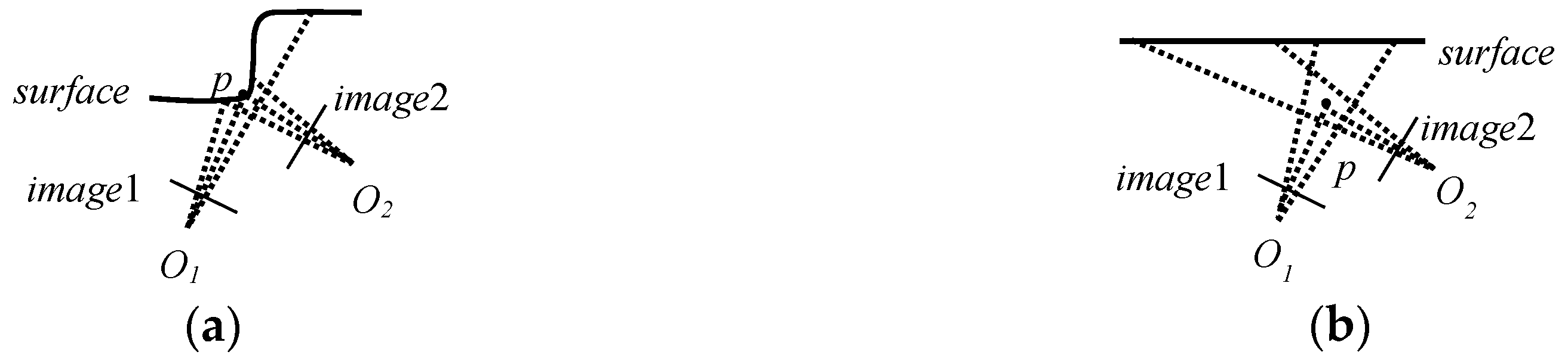
Besides outliers, occlusion can also lead to depth discontinuity. As illustrated in Figure 4a, when observed from a camera with an optical center O1, the depth around point p is discontinuous due to occlusion. When observed from another camera with an optical center O2, the discontinuity disappears. By contrast, in the case of an outlier, the depth discontinuity will always exist, regardless of viewpoints, as illustrated in Figure 4b. To distinguish these two situations, we checked the depth discontinuity of point p in every selected image. If the depth is discontinuous in the majority of the selected images (i.e., in more than sixty percent of total selected images), the point is identified as an outlier and filtered out.
2.4.3. Normal Consistency Filter
3D points within a very small region usually point in a direction with small deviation. If the normal n0 of point p is far away from the average of its neighbor points’ normal ni, as judged by dot production in Expression (21), then it should be filtered out.
In expression (21), N3 is the number of neighbor points within 3 s from point p. thdp is a threshold value.
3. Results and Discussion
3.1. Typical Results
We have tried our algorithm with good results for the reconstruction of various kinds of scenes, featuring small and big sizes, simple and complicate structures, strong and weak textures, changing illuminations, moving obstacles, occlusion, etc. The data sets were from Technical University of Denmark (DTU) benchmarks [1,2], Middlebury benchmarks [3], or captured by ourselves. Figure 5 presents some typical images from the data sets used in the experiments. The parameters for the data sets are listed in Table 2. Figure 6 gives the corresponding reconstructed color 3D point clouds observed from different viewpoints. In our experiments the reconstruction parameters were set as N1 = 150, thσ2 = 36, thd = 8s, thc = 0.3, thdp = 0.342, a1 = s, a2= 1.5s, a3 = 2s. These parameters, which were mostly for thresholds, were either fixed or changed with step s in all our experiments and worked well. The reason might be that the framework of the proposed algorithm made the reconstruction of each point relatively independent. An outlier, even if it was created and escaped exclusion by one filter in a particular situation, might hardly escape notice by another filter and subsequent initial value modification and re-optimization. In other words, it could hardly spread to other regions. Our experiments were performed on a 2.4 GHz Pentium computer. The proposed algorithm was coded in Matlab without careful optimization of the loops, the reading and writing of data files, etc. So, it took a longer time than some other state-of-the-art algorithms do, which have usually been implemented in the C language. For example, the volleyball and house model took about 4 h and 6 h, respectively. However, significant acceleration on speed is expected when the algorithm is carefully optimized and transformed into C language and further aided by parallel computation, which is our next goal.
As shown in Figure 5, the dino and volleyball were smooth with a weak texture. Yet they were reconstructed successfully as shown in Figure 6. The temple and house model bore many regions with high curvature, e.g., the pillar in the red rectangle and the antenna (about one millimeter [1,2]) in a green rectangle in Figure 5. Yet all these highly-curved surfaces and thin structures were reconstructed clearly, as can be seen in Figure 6. The lion and quadripod in Figure 6 gave examples of the reconstruction of scenes with moving pedestrians and different illumination. For example, the lion was shot in two days with different environmental light, as can be seen in the third row of Figure 5. Science hall in Figure 6 provided an example of the reconstruction of big and complicated scenes. There were moving pedestrians and moving cars, fixed cars, working LED screen and so on, as shown in the second row of Figure 5. Besides, all the images have a looking-up view direction since they were shot from the ground. The reconstructed science hall was generally complete without many error points, as can be seen in Figure 6. The good performance of our algorithm in the above examples verifies its robustness and ability to deal with different kinds of scenes.
3.2. Quantitative Evaluation and Comparison
3.2.1. Comparison of Two Initial Sparse Seed Point Extraction Methods
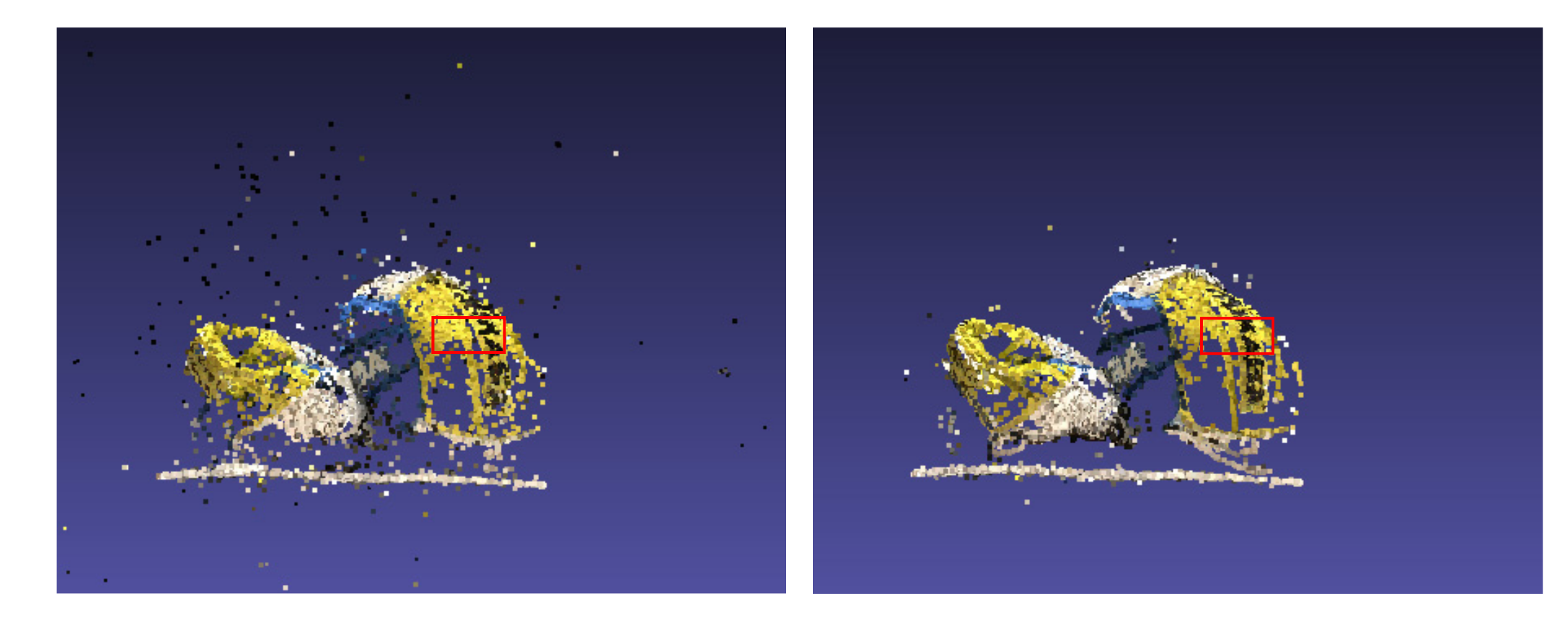
First, we compared two initial sparse seed points extraction methods. The sparse seed points for volleyball were extracted using SFM (based on SIFT) and our proposed method based on DAISY and are shown in Figure 7. The first row provides the entire view and the second row gives enlarged details of the corresponding red rectangles in the first row. From the first row, one can see that the errors in seed points when using the proposed method were much fewer. From the second row, one can see that the seed points extracted using proposed method were much denser (the number of sparse seed points extracted by the SFM method was 19,058, compared to 104,688 by the proposed method). In short, the initial sparse seed points produced by the proposed method were much denser, yet with much fewer error seed points. As a result, the reconstructed dense 3D points became more complete, which can easily be seen in Figure 8.
The quantitative evaluation results for accuracy and completeness of reconstructed dense 3D points of volleyball are listed in Table 3. As suggested by the DTU benchmarks, when evaluating accuracy, for each point p of reconstructed dense points, the nearest point is found in ground truth and its distance to the point p is calculated and marked as di. The average of all di is called mean accuracy. When all di is sorted, the middle di is called median accuracy. When evaluating completeness, for each point g of ground truth, a nearest point is found in reconstructed dense points and its distance to point g is calculated and marked as Di. The average of all the Di is called mean complete. When all Di is sorted, the middle Di is called median complete. Since an incomplete ground truth would lead to a biased evaluation, we manually cut out the same volumes from the ground truth and all dense reconstructed points where the ground truth was complete (the regions in the red rectangles in the first row of Figure 8). From Table 3, it can be seen that the mean accuracy/mean complete, 0.28/1.00 mm, of the dense 3D points expanded from sparse seed points extracted by the proposed method were significantly better than the 0.36/1.12 mm achieved by the SFM method.
3.2.2. Comparison with Other MVS Algorithms
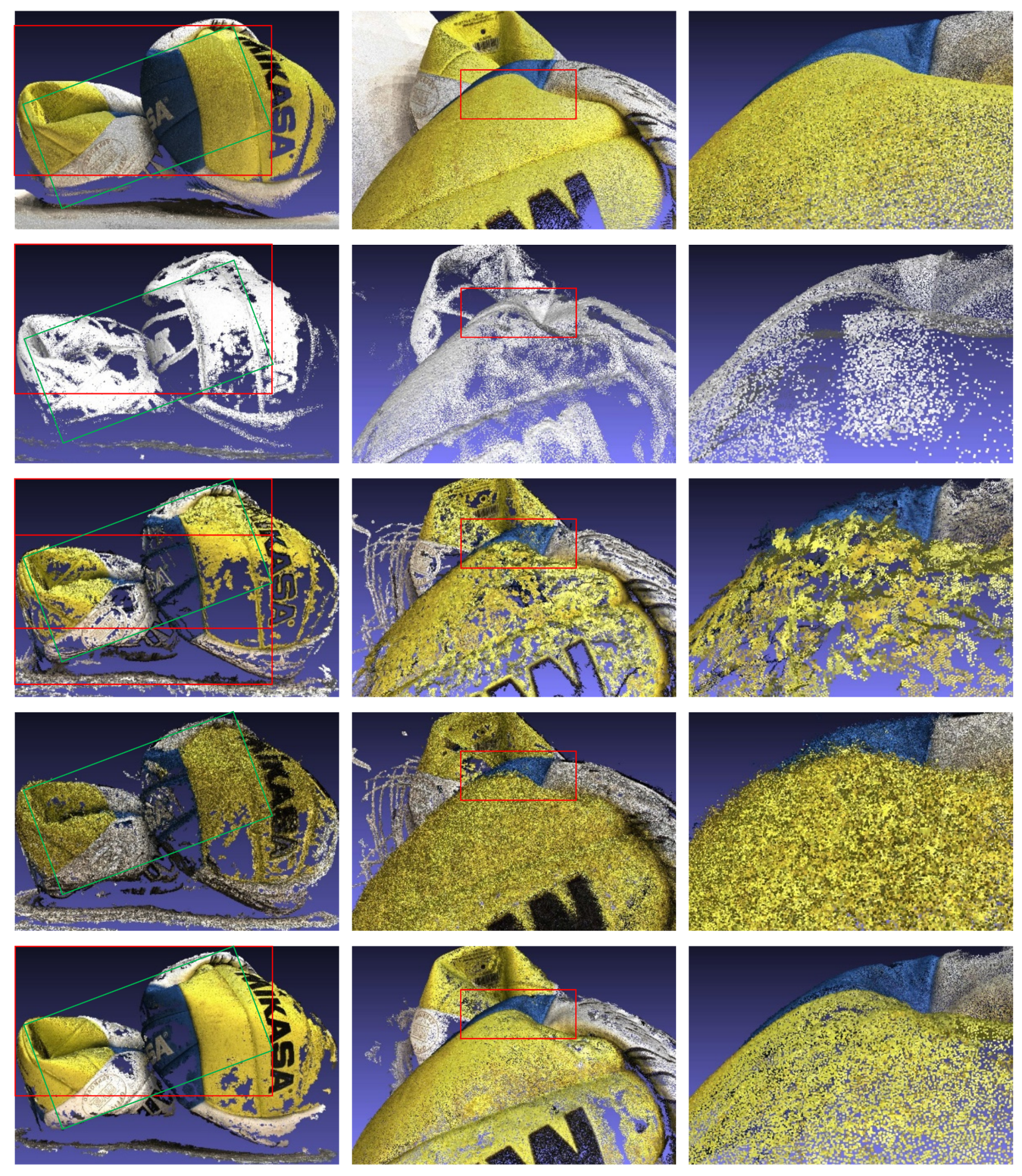
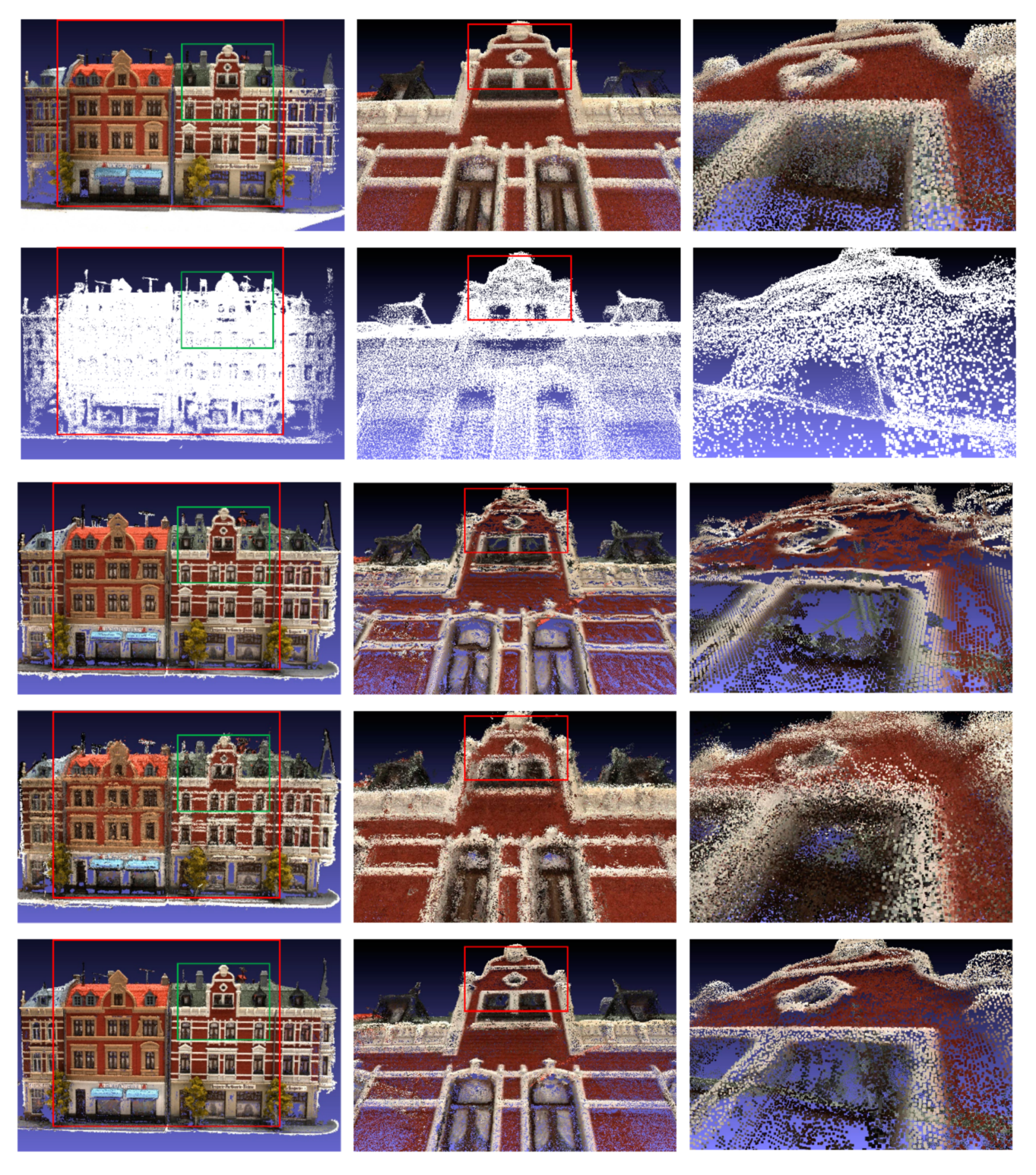
Next, we quantitatively compare the proposed algorithm with other MVS algorithms. The data sets of house model and volleyball were selected for this purpose, since their ground truths and reconstructed 3D point clouds by the DAISY algorithm [12], PMVS algorithm [16], and MRF algorithm [10] are provided by the DTU benchmarks [1,2]. As shown in the first column of Figure 9, the point cloud reconstructed by the proposed algorithm looks clean and complete. Tiny structures such as the small antenna and chimney on the roof were clearly reconstructed. Even in the enlarged views shown in the second and third columns, the proposed algorithm provided rich details with high quality, very close to the ground truth. In contrast, as can be seen from the enlarged views in the second and the third columns, the 3D point clouds reconstructed by DAISY lost some distinctive structures; 3D point clouds reconstructed by PMVS contained many tiny faults; and 3D point clouds reconstructed by MRF consisted of extremely dense points deviating obviously away from the ground truth, resulting in low accuracy.
The quantitative evaluation results for accuracy and completeness of house model are listed in Table 4. The evaluation was performed for the same volumes, manually cut out from the ground truth and all reconstructed dense points where the ground truth was complete (the regions in the red rectangles in the first column in Figure 9). From Table 4, it can be seen that, for house model, the mean accuracy of the proposed algorithm, 0.28 mm, was the same as that of the DAISY algorithm and the mean complete of the proposed algorithm, 0.41 mm, was much better than the 0.54 mm of the DAISY algorithm and 0.45 mm of the PMVS algorithm. Although the MRF algorithm had the highest completeness, its accuracy was very low. The numbers of 3D points for house model produced by DAISY, PMVS, MRF and the proposed algorithm were 1,000,782, 2,490,988, 21,918,711 and 2,029,048, respectively. These numbers reflect in some way the completeness of the algorithms.
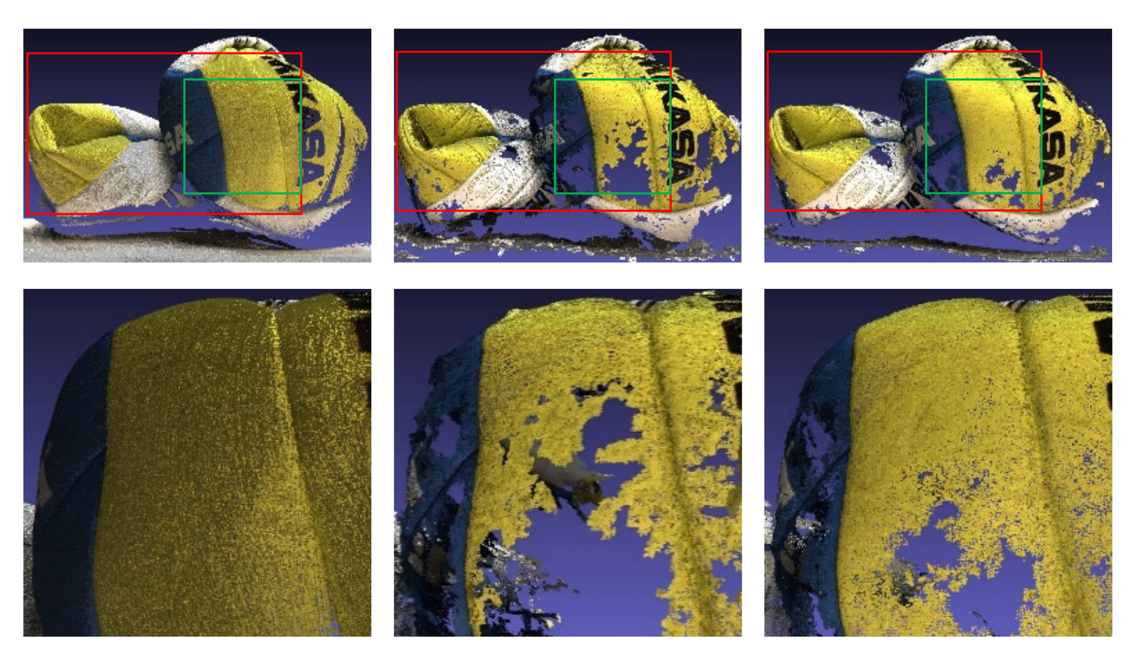
The ground truth and reconstructed 3D point clouds of volleyball are shown in Figure 10. As shown in the first column, the 3D point cloud reconstructed by the proposed algorithm appears most complete. Even in the enlarged views in the second and the third columns, it still looks smooth and continuous, very close to the ground truth. In contrast, as can be seen from enlarged views in the second and third columns, the 3D point clouds reconstructed by the DAISY algorithm has some hollow places; the 3D point clouds reconstructed by the PMVS algorithm contained many discontinuous warped pieces; the 3D point clouds reconstructed by MRF algorithm were too dense to provide good accuracy.
The quantitative evaluation results for volleyball are listed in Table 5. The evaluation was performed for the same volumes, manually cut out from the ground truth and all reconstructed dense points where the ground truth was complete (the regions in the red rectangles in the first column in Figure 10). From Table 5, it can be seen that the mean accuracy of the reconstructed 3D point cloud by the proposed algorithm, 0.28 mm, was very close to the highest, 0.27 mm by the DAISY algorithm and the mean complete of the proposed algorithm, 0.99 mm, was much better than the 2.19 mm of the DAISY algorithm and the 1.52 mm of the PMVS algorithm. The number of 3D points, 7,451,571, produced by the MRF algorithm was much higher than the number, 4,444,883, of the ground truth. Due to this redundancy, the completeness of the MRF algorithm was the highest, although its accuracy was low. The number of 3D points produced by DAISY, PMVS and the proposed algorithm were 469,749, 1,383,713 and 1,356,621, respectively.
As can be seen from the enlarged views of reconstructed 3D point clouds, our algorithm provided fine reconstruction quality. According to the quantitative evaluation results, the DAISY algorithm attained the highest accuracy at the cost of a reduced completeness. We guess that the reason for it producing the smallest number of 3D points is that it keeps only reliable 3D points. These points are usually at regions with enough texture. In contrast, the MRF algorithm generated the highest completeness at the cost of a much-reduced accuracy. We guess that the reason for it producing the largest number of 3D points is that it integrates the depths without careful selection. In addition, it uses NCC for window-based matching, which is inferior to the DAISY descriptor. We extended the framework of feature expansion algorithm by an additional step for initial value modification and made important improvements to other existing steps, which is why our algorithm outperforms PMVS in terms of both accuracy and completeness. We demonstrated that through feature expansion, many places with weak texture might be reconstructed with high accuracy. The accuracy averaged over the entire reconstructed area is still on par with the highest one of Tola.
4. Conclusions
This paper presented a novel multi-view stereo algorithm via homogeneous direct spatial expansion. To attain high accuracy and completeness, the proposed algorithm extended the framework of feature expansion algorithm by an additional step for initial value modification and improved other existing steps by many unique measures. For example, to improve reconstruction completeness it extracted initially sparse seed points using the high-performance DAISY descriptor, which increased the number of initial sparse seed by a number of times; to ensure reconstruction accuracy it conducted initial value modification via the conditional-double-surface-fitting method before optimization, and adaptive consistency filtering of outliers after optimization; to enhance efficiency it adopted an expansion strategy of homogeneous direct spatial expansion and a processing strategy based on a multi-level image pyramid. As demonstrated by experiments, owing to the above measures, the proposed algorithm attained very high reconstruction completeness and accuracy. The local and parallel processing nature of the proposed algorithm makes it suitable for dealing with various kinds of scenes, featuring small and big sizes, simple and complicated structures, strong and weak textures, changing illuminations, moving obstacles, occlusion, etc.
Acknowledgments
This work was supported in part by the National Natural Science Foundation of China under Grant No. 11605071 and in part by the Aid program for Science and Technology Innovative Research Team in Higher Educational Institutions of Hunan Province, China.
Author Contributions
Zhiyang Li and Yalan Li conceived the experiments; Yalan Li designed and performed the experiments; Zhiyang Li and Yalan Li analyzed the data and prepared the paper.
Conflicts of Interest
The authors declare no conflict of interest.
References
- Aanæs, H.; Jensen, R.R.; Vogiatzis, G.; Tola, E.; Dahl, A.B. Large-scale data for multiple-view stereopsis. Int. J. Comput. Vis. 2016, 120, 153–168. [Google Scholar] [CrossRef]
- Jensen, R.; Dahl, A.; Vogiatzis, G.; Tola, E.; Aanaes, H. Large Scale Multi-view Stereopsis Evaluation. In Proceedings of the 27th IEEE Conference on Computer Vision and Pattern Recognition, Columbus, OH, USA, 23–28 June 2014; pp. 406–413. [Google Scholar]
- Seitz, S.M.; Curless, B.; Diebel, J.; Scharstein, D.; Szeliski, R. A Comparison and Evaluation of Multi-view Stereo Reconstruction Algorithms. In Proceedings of the 2006 IEEE Computer Society Conference on Computer Vision and Pattern Recognition, New York, NY, USA, 17–22 June 2006; pp. 519–528. [Google Scholar]
- Snavely, N.; Seitz, S.M.; Szeliski, R. Photo tourism: exploring photo collections in 3D. ACM Trans. Graph. 2006, 25, 835–846. [Google Scholar] [CrossRef]
- Seitz, S.M.; Dyer, C.R. Photorealistic scene reconstruction by voxel coloring. Int. J. Comput. Vis. 1999, 35, 151–173. [Google Scholar] [CrossRef]
- Kutulakos, K.N.; Seitz, S.M. A theory of shape by space carving. Int. J. Comput. Vis. 2000, 38, 199–218. [Google Scholar] [CrossRef]
- Jin, H.; Soatto, S.; Yezzi, A.J. Multi-view stereo reconstruction of dense shape and complex appearance. Int. J. Comput. Vis. 2005, 63, 175–189. [Google Scholar] [CrossRef]
- Vogiatzis, G.; Hernandez, C.; Torr, P.H.; Cipolla, R. Multiview stereo via volumetric graph-cuts and occlusion robust photo-consistency. IEEE Trans. Pattern Anal. Mach. Intell. 2007, 29, 2241–2246. [Google Scholar] [CrossRef] [PubMed]
- Kolmogorov, V.; Zabih, R. Multi-camera Scene Reconstruction via Graph Cuts. In Proceedings of the 7th European Conference on Computer Vision, Copenhagen, Denmark, 28–31 May 2002; pp. 82–96. [Google Scholar]
- Goesele, M.; Curless, B.; Seitz, S.M. Multi-view Stereo Revisited. In Proceedings of the 2006 IEEE Computer Society Conference on Computer Vision and Pattern Recognition, New York, NY, USA, 17–22 June 2006; pp. 2402–2409. [Google Scholar]
- Campbell, N.D.; Vogiatzis, G.; Hernandez, C.; Cipolla, R. Using Multiple Hypotheses to Improve Depth-maps for Multi-view Stereo. In Proceedings of the 10th European Conference on Computer Vision, Marseille, France, 12–18 October 2008; pp. 766–779. [Google Scholar]
- Tola, E.; Strecha, C.; Fua, P. Efficient large-scale multi-view stereo for ultra high-resolution image sets. Mach. Vis. Appl. 2012, 23, 903–920. [Google Scholar] [CrossRef]
- Otto, G.P.; Chau, T. “Region-growing” algorithm for matching of terrain images. Image Vis. Comput. 1989, 7, 83–94. [Google Scholar] [CrossRef]
- Goesele, M.; Snavely, N.; Curless, B.; Hoppe, H.; Seitz, S.M. Multiview Stereo for Community Photo Collections. In Proceedings of the 11th International Conference on Computer Vision, Rio de Janeiro, Brazil, 14–20 October 2007. [Google Scholar] [CrossRef]
- Habbecke, M.; Kobbelt, L. A Surface-growing Approach to Multi-view Stereo Reconstruction. Proceedings of 2007 IEEE Computer Society Conference on Computer Vision and Pattern Recognition, Minneapolis, MN, USA, 17–22 June 2007; pp. 1–6. [Google Scholar]
- Furukawa, Y.; Ponce, J. Accurate, dense, and robust multiview stereopsis. IEEE Trans. Pattern Anal. Mach. Intell. 2010, 32, 1362–1376. [Google Scholar] [CrossRef] [PubMed]
- Kazhdan, M.; Bolitho, M.; Hoppe, H. Poisson Surface Reconstruction. In Proceedings of the fourth Eurographics Symposium on Geometry Processing, Cagliari, Italy, 26–28 June 2006; pp. 61–70. [Google Scholar]
- Chen, L.C.; Hoang, D.C.; Lin, H.I.; Nguyen, T.H. Innovative methodology for multi-view point cloud registration in robotic 3D object scanning and reconstruction. Appl. Sci. 2016, 6, 132. [Google Scholar] [CrossRef]
- Strecha, C.; Fransens, R.; Gool, L.V. Combined depth and outlier estimation in multi-view stereo. In Proceedings of the 2006 IEEE Computer Society Conference on Computer Vision and Pattern Recognition, New York, NY, USA, 17–22 June 2006; pp. 2394–2401. [Google Scholar]
- Tola, E.; Lepetit, V.; Fua, P. DAISY: An efficient dense descriptor applied to wide-baseline stereo. IEEE Trans. Pattern Anal. Mach. Intell. 2010, 32, 815–830. [Google Scholar] [CrossRef] [PubMed]
- Frahm, J.M.; George, P.; Gallup, D.; Johnson, T.; Raguram, R.; Wu, C.; Jen, Y.H.; Dunn, E.; Clipp, B.; Lazebnik, S.; et al. Building Rome on A Cloudless Day. In Proceedings of the 11th European Conference on Computer Vision, Heraklion, Crete, Greece, 5–11 September 2010; pp. 368–381. [Google Scholar]
- Rashidi, A.; Brilakis, I.; Vela, P. Generating Absolute-Scale Point Cloud Data of Built Infrastructure Scenes Using a Monocular Camera Setting. J. Comput. Civ. Eng. 2015, 29, 04014089. [Google Scholar] [CrossRef]
- Rashidi, A.; Fathi, H.; Brilakis, I. Innovative Stereo Vision-Based Approach to Generate Dense Depth Map of Transportation Infrastructure. Transp. Res. Rec.: J. Transp. Res. Board 2011, 2215, 93–99. [Google Scholar] [CrossRef]
- Brilakis, I.; Fathi, H.; Rashidi, A. Progressive 3D Reconstruction of Infrastructure with Videogrammetry. J. Autom. Constr. 2011, 20, 884–895. [Google Scholar] [CrossRef]
- Gruen, A.W. Adaptive least squares correlation: A powerful image matching technique. S. Afr. J. Photogramm. Remote Sens. Cartogr. 1985, 14, 175–187. [Google Scholar]
- Fuhrmann, S.; Langguth, F.; Moehrle, N.; Waechter, M.; Goesele, M. Mve-an image-based reconstruction environment. Comput. Gr. 2015, 53, 44–53. [Google Scholar] [CrossRef]
- Wu, C. Towards Linear-time Incremental Structure From Motion. Proceedings of 2013 International Conference on 3D Vision, Seattle, WA, USA, 29 June–1 July 2013; pp. 127–134. [Google Scholar]
- Lowe, D.G. Distinctive image features from scale-invariant keypoints. Int. J. Comput. Vis. 2004, 60, 91–110. [Google Scholar] [CrossRef]
- Fischler, M.A.; Bolles, R.C. Random sample consensus: A paradigm for model fitting with applications to image analysis and automated cartography. Commun. ACM 1981, 24, 381–395. [Google Scholar] [CrossRef]
- Möller, T.; Hughes, J.F. Efficiently building a matrix to rotate one vector to another. J. Gr. Tools 1999, 4, 1–4. [Google Scholar] [CrossRef]
Figure 1.
Workflow diagram of the proposed algorithm.

Figure 2.
Illustration of the principle of homogeneous direct spatial expansion: (a) Direct expansion of seed points in 3D space along tangent planes; (b) The initial positions of points for the first three iterations of expansion. Black, green and yellow points stand for the first, second and third iteration, respectively. For convenience, these points are drawn on the same plane with equal separation; actually, after optimization, they would sit on different planes with slightly different separations.

Figure 3.
Double surface fitting. Solid line: object surface. Dotted line: fitted surface on the first iteration. Dashed line: fitted surface on the second iteration. Solid black points: reconstructed 3D points. p1~3: 3D points with large residual error.
Figure 3.
Double surface fitting. Solid line: object surface. Dotted line: fitted surface on the first iteration. Dashed line: fitted surface on the second iteration. Solid black points: reconstructed 3D points. p1~3: 3D points with large residual error.
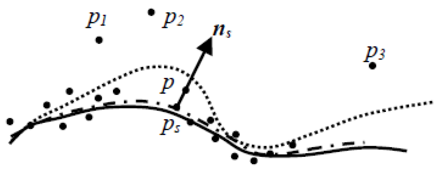
Figure 4.
Two kinds of depth discontinuities: (a) Depth discontinuity caused by occlusion; (b) Depth discontinuity caused by an outlier.
Figure 4.
Two kinds of depth discontinuities: (a) Depth discontinuity caused by occlusion; (b) Depth discontinuity caused by an outlier.

Figure 5.
Typical images for data sets used in experiments. Data sets in the first row from left to right are dino (one image), temple (one image), volleyball (two images) and house model (two images). The data set in the second row is science hall. Data sets in the third row from left to right are lion and quadripod, each with three images.
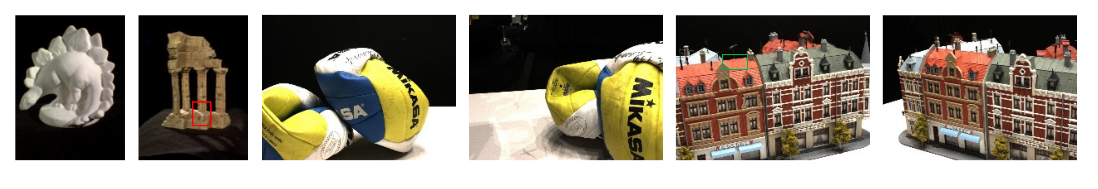
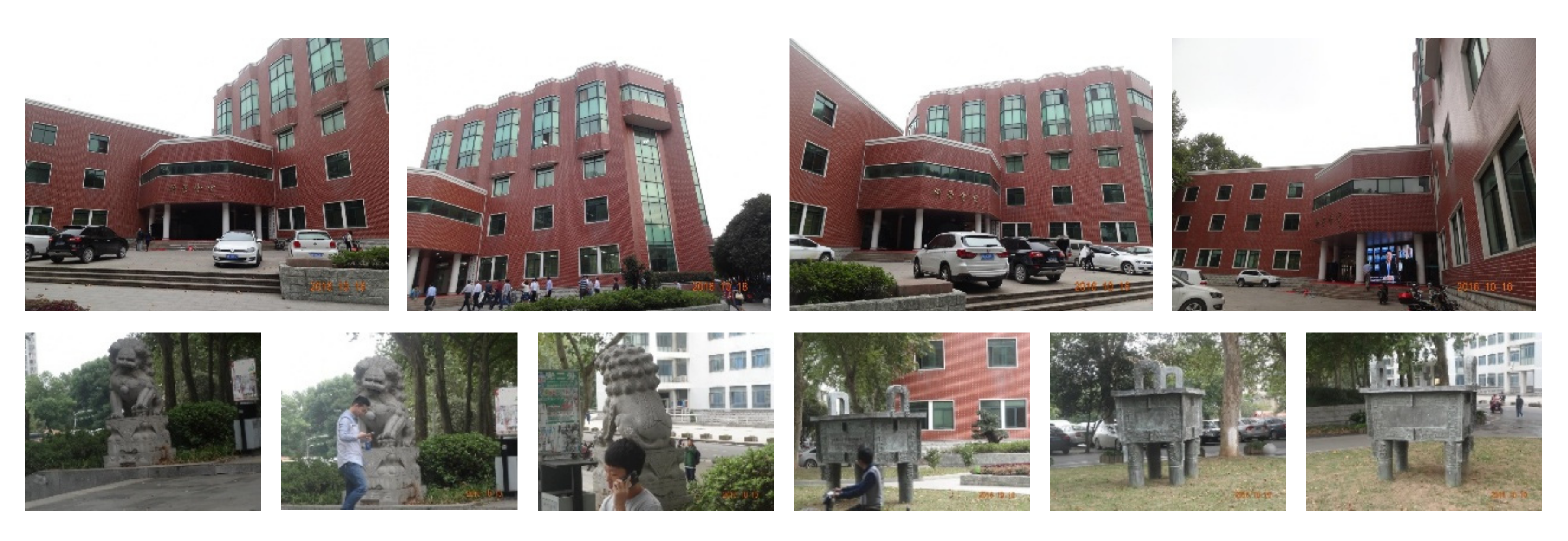
Figure 6.
Some reconstructed 3D colored point clouds with different viewpoints. In the first row from left to right: dino (two views), temple (two views), and volleyball (one view). In the second row from left to right are house model and science hall. In the third row from left to right are lion and quadripod each with two views.
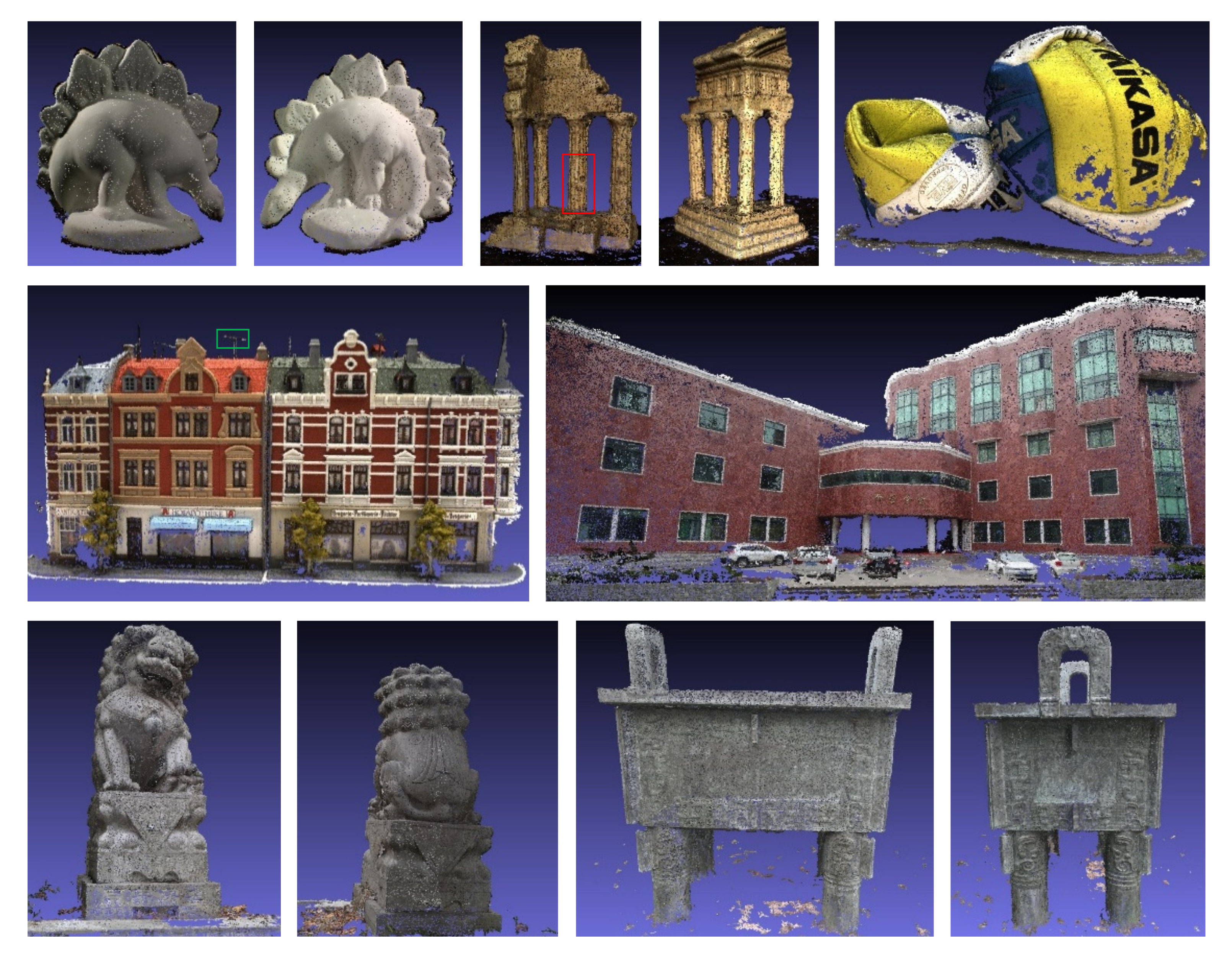
Figure 7.
Sparse seed points of volleball extracted by the SFM method and the proposed method. Each row from left to right: sparse seed points extracted by the SFM method, sparse seed points extracted by the proposed method. The second row presents the enlarged details of the corresponding red rectangles in the first row.

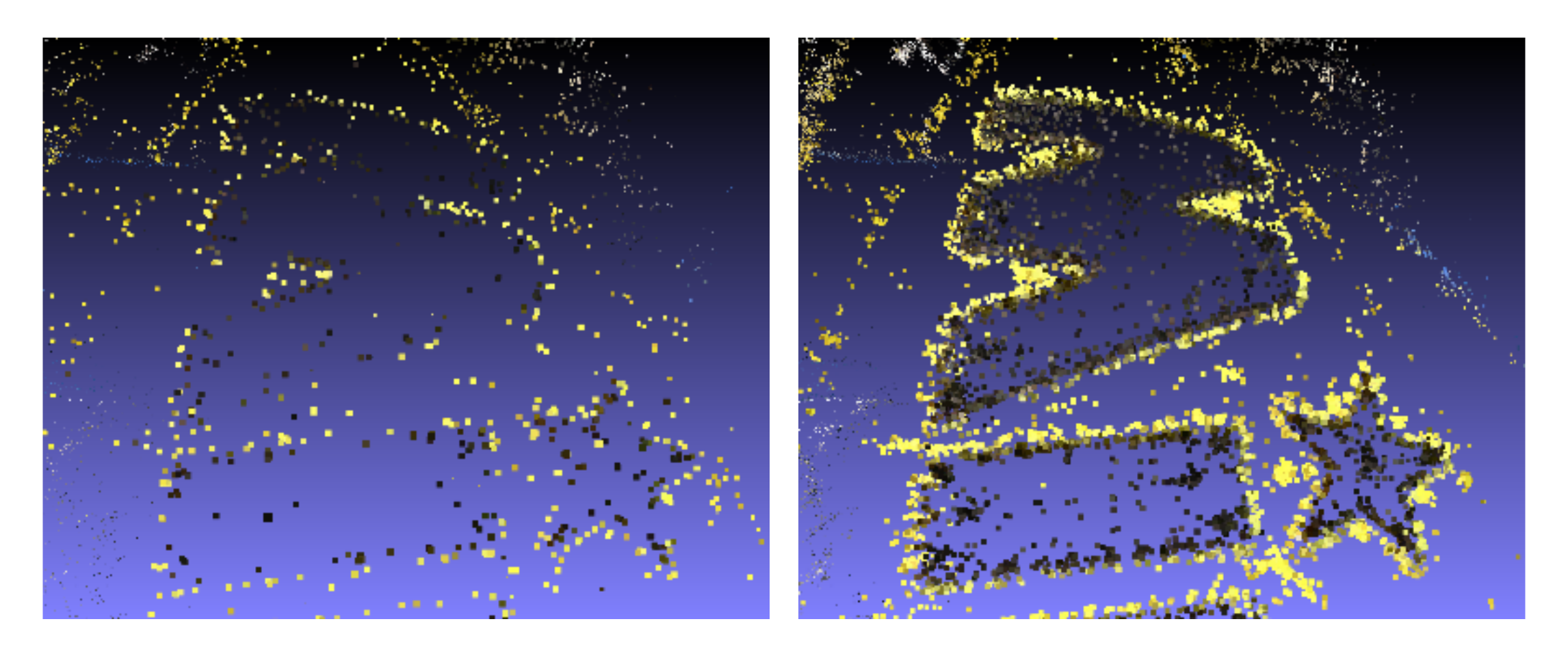
Figure 8.
Dense 3D point clouds of volleyball expanded from sparse seed points extracted by the SFM and proposed methods. Each row from left to right: ground truth, dense points following the SFM method, dense points following the proposed method. The first row presents the entire images and the second row presents enlarged details within the green rectangles of the first row.

Figure 9.
The ground truth and reconstructed 3D point clouds of house model. From top row to bottom row: ground truth, 3D points as reconstructed by DAISY, PMVS, MRF, and the proposed algorithm. The second column shows enlarged views of the corresponding green rectangles in the same row of the first column, whereas the third column shows enlarged views of the corresponding red rectangles in the same row of the second column.

Figure 10.
The ground truth and reconstructed 3D point clouds of volleyball. From top row to bottom row: ground truth, reconstructed 3D points by DAISY, PMVS, MRF, and the proposed algorithm. The second column shows enlarged views of the corresponding green rectangles in the same row of the first column, whereas the third column shows enlarged views of the corresponding red rectangles in the same row of the second column.

Table 1.
A few selected works on 3D reconstruction based on photometry.
| Methods | Authors-Year | Technical Features and Sample Result |
|---|---|---|
| Volume based algorithms | Seitz et al., 1999 [5] | Voxel coloring. Camera positions were constrained to handle occlusion problem. A dinosaur toy was reconstructed with 71,841 grids out of 166 × 199 × 233 initial grids. |
| Kutulakos et al., 2000 [6] | Space carving. Camera positions are not constrained. Occlusion problem was solved by multi-pass plane sweep. A hand with 112k voxels was reconstructed. | |
| Jin et al., 2005 [7] | Shape evolution. Discrepancy function was minimized by level set method. A highly specular statue was reconstructed. | |
| Vogiatzis et al., 2007 [8] | Volumetric graph-cut. Global cost functional is minimized to obtain shape and avoid occlusion. Temple data set was reconstructed. | |
| Depth-map fusion algorithms | Kolmogorov et al., 2002 [9] | Energy minimization by graph cut. An energy formulation was given to model photo-consistency, smoothness and visibility at the same time. Four 384 × 288 depth maps for Tsukuba data were computed. |
| Goesele et al., 2006 [10] | Window-based matching. A depth map was reconstructed for each image and only those points with high confidence based on Normalized Cross Correlation (NCC) were selected. The nskulla dataset was reconstructed. | |
| Campbell1 et al., 2008 [11] | Markov Random Field (MRF ) optimization. A reliable depth was selected from one of NCC peaks and unknown labels were attached to outliers so that small matching window can be used to gain high accuracy. Depth maps for the Cones data set were computed. | |
| Tola et al., 2012 [12] | DAISY descriptor matching. Dense point clouds were found from image pairs and only those points with the highest expected precision were retained. EPFL campus was reconstructed using 31 40-Megapixel images in 14.2 min and the final point cloud contains 11.3 million points. | |
| Feature expansion algorithms | Otto et al., 1989 [13] | Area-based matching and expansion. A “best-first” strategy was adopted. 30 m Digital Elevation Model (DEM ) was computed from a pair of 240 × 240 terrain images with a mean difference of −3.716 m corresponding to matching accuracy possibly as low as 0.1 pixels. |
| Goesele et al., 2007 [14] | Window-based matching and expansion. A sequential expansion was performed based on a priority queue. Images were intelligently chosen at a per-view and per-pixel level. St. Peter’s cathedral was reconstructed from 151 Internet images by 50 photographers. | |
| Habbecke et al., 2007 [15] | Disk-based matching and expansion. New planar disks were expanded at a fraction (20%) of the parent disk’s minimal radius (100 pixel). A statue of a Chinese warrior was reconstructed with 264k disks. | |
| Furukawa et al., 2010 [16] | Patch-based matching and expansion. All the patches were expanded with the same priority. Outliers were filtered out based on visibility and weak neighborhood regulation. Many small objects and large scenes were reconstructed. |
Table 2.
Parameters of datasets and expansion step s.
| Dataset Name | Image Number | Image Size | s |
|---|---|---|---|
| dino | 48 | 640 × 480 | 0.006 |
| temple | 47 | 640 × 480 | 0.003 |
| volleyball | 49 | 1600 × 1200 | 0.01 |
| house model | 49 | 1600 × 1200 | 0.0085 |
| science hall | 65 | 1152 × 864 | 0.06 |
| lion | 42 | 1152 × 864 | 0.009 |
| quadripod | 45 | 1152 × 864 | 0.01 |
Table 3.
Evaluation results (mm) for volleyball with different initial sparse seed extraction methods.
Table 3.
Evaluation results (mm) for volleyball with different initial sparse seed extraction methods.
| Method | Mean Complete | Mean Accuracy | Med Complete | Med Accuracy |
|---|---|---|---|---|
| SFM | 1.12 | 0.36 | 0.29 | 0.18 |
| Proposed | 1.00 | 0.28 | 0.28 | 0.16 |
Table 4.
Evaluation results (mm) for house model by different MVS algorithms.
| Method | Mean Complete | Mean Accuracy | Med Complete | Med Accuracy | Point Number |
|---|---|---|---|---|---|
| DAISY | 0.54 | 0.28 | 0.40 | 0.20 | 1,000,782 |
| PMVS | 0.45 | 0.37 | 0.37 | 0.25 | 2,490,988 |
| MRF | 0.17 | 0.63 | 0.15 | 0.41 | 21,918,711 |
| Proposed | 0.41 | 0.28 | 0.33 | 0.19 | 2,029,048 |
Table 5.
Evaluation results (mm) for volleyball by different MVS algorithms.
| Method | Mean Complete | Mean Accuracy | Med Complete | Med Accuracy | Point Number |
|---|---|---|---|---|---|
| DAISY | 2.19 | 0.27 | 0.51 | 0.15 | 469,749 |
| PMVS | 1.52 | 0.51 | 0.41 | 0.35 | 1,383,713 |
| MRF | 0.93 | 0.66 | 0.19 | 0.47 | 7,451,571 |
| Proposed | 0.99 | 0.28 | 0.28 | 0.16 | 1,356,621 |
© 2017 by the authors. Licensee MDPI, Basel, Switzerland. This article is an open access article distributed under the terms and conditions of the Creative Commons Attribution (CC BY) license (http://creativecommons.org/licenses/by/4.0/).
Share and Cite
MDPI and ACS Style
Li, Y.; Li, Z. A Multi-View Stereo Algorithm Based on Homogeneous Direct Spatial Expansion with Improved Reconstruction Accuracy and Completeness. Appl. Sci. 2017, 7, 446. https://doi.org/10.3390/app7050446
AMA Style
Li Y, Li Z. A Multi-View Stereo Algorithm Based on Homogeneous Direct Spatial Expansion with Improved Reconstruction Accuracy and Completeness. Applied Sciences. 2017; 7(5):446. https://doi.org/10.3390/app7050446
Chicago/Turabian StyleLi, Yalan, and Zhiyang Li. 2017. "A Multi-View Stereo Algorithm Based on Homogeneous Direct Spatial Expansion with Improved Reconstruction Accuracy and Completeness" Applied Sciences 7, no. 5: 446. https://doi.org/10.3390/app7050446
Note that from the first issue of 2016, this journal uses article numbers instead of page numbers. See further details here.