
Jointly Production and Correlated Maintenance Optimization for Parallel Leased Machines

1
Laboratory of Industrial Engineering Production and Maintenance, University of Lorraine, UFR MIM, île du Saulcy-BP 50128, 57045 Metz, France
2
ICN Business School, 54003 Nancy-Metz, France
*
Author to whom correspondence should be addressed.
Appl. Sci. 2017, 7(5), 461; https://doi.org/10.3390/app7050461
Submission received: 8 March 2017
/
Revised: 23 April 2017
/
Accepted: 25 April 2017
/
Published: 30 April 2017
Abstract
:This paper deals with a preventive maintenance strategy optimization correlated to production for a manufacturing system made by several parallel machines under lease contract. In order to minimize the total cost of production and maintenance by reducing the production system interruptions due to maintenance activities, a correlated group preventive maintenance policy is developed using the gravity center approach (GCA). The aim of this study is to determine an economical production plan and an optimal group preventive maintenance interval Tn at which all machines are maintained simultaneously. An analytical correlation between failure rate of machines and production level is considered and the impact of the preventive maintenance policy on the production plan is studied. Finally, the proposed maintenance policy GPM is compared with an individual simple strategy approach IPM in order to illustrate its efficiency.
1. Introduction
In classical scheduling strategies, it is generally assumed that the system is available to produce at all times, which is wrong since machines are subject to failures and breakdowns. Finding the optimal production plan taking into account the maintenance strategy is then necessary to increase the economic returns of a firm and to handle backorders. In the frame of production and maintenance optimization, Mohamed-Salah et al. [1] presented a simultaneous optimization model of production flow and preventive maintenance actions taking into account the interaction between both services. The authors considered a system composed by a single unit producing one type of product in order to satisfy a constant demand. They proposed a model for the maintenance strategy based on the level of the inventory and the age of the machine. They minimized firstly the total maintenance cost in order to obtain the optimal age of preventive maintenance actions and then established the expression of the total costs associated with the holding stock and unsatisfied demands. The combination between both costs allows minimizing a global cost function integrating simultaneously the maintenance, the inventory as well as the unsatisfied demands costs in order to obtain an optimal security stock.
So many works have treated the joint optimization of production and maintenance strategies. Some of these works were devoted to study the case of restricted and simple systems composed by only one machine while others were interested in more complex systems composed by several machines whose number is fixed and known during the production horizon. Finding the optimal production and maintenance policies, by minimizing the total costs, becomes then more complex when the number of machines is variable. Chelbi et al. [2] developed an optimization model for a production system composed by one machine producing with a constant cadence in order to satisfy the demand. Since the machine is prone to random failures, corrective and preventive maintenance actions are performed at periodically dates T, 2T... They proposed the construction of a security stock S to meet the demand during the period of machine shutdown. The objective of this work is to determine simultaneously the optimal periodicity of preventive maintenance actions T* as well as the optimal stock level S* which minimize the average total cost of maintenance, inventory and unsatisfied demands. Rezg et al. [3] presented an analytical model for a production line composed by n machines which have an identical production rate to satisfy a constant demand. Simulation and genetic algorithms are the approaches used to determine the optimal preventive maintenance dates and stock levels. Some authors treated the coupling between production and maintenance considering new constraints like subcontracting ([4] and [5]). Dellagi et al. [4] developed new maintenance policies while coupling maintenance and production under subcontracting constraint. To satisfy the customer demand, subcontracting is sometimes needed in order to hedge against shortage. Concerning reliability, the authors considered a constant failure rate for the subcontractor’s machine and an optimal maintenance planning for the principal machine by proposing an improved maintenance policy which takes into account the constraint of subcontracting. Zhao et al. [6] considered an order-dependent failure and developed an iterative method to solve the problem for a single-machine system. The model developed by Li et al. [7] optimizes jointly the production and the maintenance schedules for a single machine system taking into account both the quality robustness and the solution robustness. An approach based on a three-phase heuristic is used in order to find the optimal solution. Cui et al. [8] considered the quality aspect of the system in order to integrate the lot-sizing problem to the preventive maintenance scheduling. A system composed by M defined machines was considered and the production and maintenance schedules were determined using a genetic algorithm. The system undergoes quality inspections which are accompanied with adjustment and calibration activities to confirm that the machine will start the next production interval in its normal state. If inspection detected that a shift has occurred (the machine is in a degraded state), all items produced on the related machine interval need to be checked, and defective items should be separated. Fakher et al. [9] studied a production system with a decreasing production capacity over time and determined its production and maintenance plans. Yalaoui et al. [10] studied a multi-product single machine system, which is subject to random failures. They minimized the sum of the total production and maintenance costs related to inventory, backorder, production, set-up, preventive maintenance, and minimal repair under demand satisfaction and machine capacities constraints.
Some works have dealt with the group maintenance scheduling optimization; we can mention Hnaien et al. [11] which is one of the first works to deal with this type of problem. The authors considered a system composed by n independent identical machines which fail separately and developed a nomograph for all machines which allows determining the time for repair as well as the total maintenance cost. The group maintenance activity is performed when a certain time interval elapsed. Okumoto et al. [12] considered two time-intervals (0, T) and (T, T + W) during which failures are either removed by minimal repairs or removed by replacement or are left idle. During the first interval (0, T), if a unit fails at age y it is either replaced by a new one with a probability p(y) or it undergoes a minimal repair with a probability 1-p(y). During the second interval (T, T + W), no replacement is performed until the group maintenance; failures, when occurred, are either removed by minimal repairs or are left idle. The group maintenance strategy in this work is performed at time T + W or upon the kth idle whichever comes first. More recent works have also dealt with the group maintenance optimization problem; Sheu et al. [13] studied the impact of opportunistic maintenance on the effectiveness of condition-based maintenance. They considered a system composed by three components mounted in series and varied few elements such as the number of components, the length of the opportunistic zone and used a dynamic grouping in which group maintenance activity is carried out only for the non-failed components that are in the opportunistic zone. Koochaki et al. [14] developed a group maintenance policy for parallel machines. Their model allows determining jointly the optimal maintenance frequencies, the optimal positions of the maintenance activities and the optimal job sequence. An algorithm in which the authors fixed the maintenance frequencies is provided in order to solve the problem. In the work of Yang et al. [15], the authors used a genetic algorithm in order to develop an optimum group maintenance schedule of a water-distributed network. A judgment matrix based on the adjacent geographical distribution of the pipelines is used to control the searching space of the maintenance grouping optimization model. Do et al. [16] developed a dynamic maintenance grouping approach for a multi-components system using two optimization algorithms (genetic and multifit). The developed approach allows obtaining an optimal maintenance schedule taking into account the availability of repairmen constraints. Shafiee et al. [17] studied the case of a multi-components system and proposed an age-based group maintenance policy that provides an optimal group maintenance time T* by minimizing the average long-run maintenance cost. Concerning joint optimization of production and group maintenance policies, Xiao et al. [18] considered a series system of machines processing different types of jobs. They used a genetic algorithm in order to find the optimal group preventive maintenance policy (the optimal preventive maintenance interval) as well as the assignment of jobs on machines. Results are compared to an individual preventive maintenance policy in order to show the effectiveness of the used approach. In the work of Renna et al. [19], the author considered a manufacturing system composed by a given number of cells consisting of a given number of machines which have to satisfy a random demand. The impact of preventive maintenance on the manufacturing system’s performance is investigated. Static and dynamic environments were also taken into account in order to study the performance of the manufacturing system. The author used a multi-agents architecture to illustrate the scheduling problem. A discrete event simulation using Arena platform was used in order to simulate the manufacturing environment. The results found by the author show that changes and working time uncertainty have a significant effect on the performance of the manufacturing system since they lead to major benefits when a preventive maintenance policy is used. Zhang et al. [20] proposed a model for a group preventive maintenance optimization using the failure effects analysis. The authors considered a workshop composed by several machines which have two types of state: either good or failure state. For each state, they determined the average of failure effect using the Monte-Carlo simulation taking into account the different considered variables. The authors have considered a non-negligeable time for repair which leads to production losses.
All aforementioned works in the frame of group maintenance strategy considered either a series system where failed equipment leads to a whole system breakdown or a fixed number of components (machines) in order to solve this kind of problem. However, and in the case of leased equipment, the number of machines to use can vary from a period to another according to the customers’ demand. Also, few works have studied the case of a parallel machines system, in which, even if a machine fails, the system continues to perform its production process, unlike the case of a series system where a failed machine leads to the whole system breakdown. The problem becomes harder to resolve when the number of machines and the customer’s demands are dynamic from a production period to another and depend on each other. This paper shows that it has a novelty and originality relative to this type of problem since it investigates the case study of a production system composed by a variable number of identical parallel machines under lease contract. can vary from a period to another according to a random customer’s demand. Each machine has a unique processing time in regular work time; if any machine achieves certain duration in regular work time, then it can perform an extra work time in order to satisfy the random demand. The degradation rate of these machines is correlated with the production during a finite horizon. The other added value of this study consists of the establishment of a new method of correlated group preventive maintenance policy based on the gravity center approach (GCA). We put emphasis on the originality of this work since it is characterized by the use of new approaches and an analytical study taking into consideration the influence of the production rates on the system’s degradation degree. Minimizing the cost of production and correlated preventive maintenance provides the optimal number of machines to be leased, the quantity to produce by each one and the optimal interval of group preventive maintenance.
The remainder of this paper is as follows: Section 2 is devoted to describe the problem. In Section 3, we formulate the joint optimization problem and give the objective function. The different approaches, techniques and steps used to solve the problem are shown in Section 4. Section 5 deals with a numerical example in which we compare our results to an individual maintenance strategy for the same studied system. Finally, the conclusion of the paper is given in Section 6.
2. Problem Description and Industrial Context
As mentioned above, in the present work we focus on a parallel manufacturing system composed by several identical machines. We referred, in this study, to a real case of a company specialized in metal and steel parts manufacturing. When the pieces ordered by customers are of a complex shape, the technology used by this firm is based on laser machining tools used to cut materials (steel in most cases) with extreme precision in order to obtain a high-quality product. Due to the expensiveness of laser tools, and since the company does not use this type of equipment regularly, the managers use to lease these machines in order to satisfy some customers’ orders. Given the fluctuation of demand, the number of the leased machines does not remain constant and may vary from one period to another. Also, given the complexity of the technology used by these machines, maintenance activities are performed by specialists, generally from the lessor company. Leasing contracts are generally concluded for one year, or more, depending on the use of the equipment. The leasing fees are paid monthly at the debut of each period. Group maintenance activity for this kind of systems is then of a huge importance since it allows the lessee to avoid unavailability of repairmen, which is most frequently encountered in the case of an individual maintenance strategy.
Inspired from Hajej et al. [21], and in order to take into account production planning while minimizing maintenance cost, we put emphasis on degradation function of each available machine according to its production rate.
We consider the production system that has to satisfy a random demand of one type of product. This demand fluctuates according to a normal distribution with mean and variance given respectively by and . The number of machines to be leased depends on the customer’s demand and varies from one production period to another. Processing time for each machine is also variable: in fact a machine can operate for a maximum duration in regular work time denoted by , once exceeded this value, a machine can operate up to of extra time work (overtime). A periodic group maintenance strategy is performed to all machines in order to reduce the probability of failure. We put emphasis on the complexity of jointly determining production and maintenance plans for this kind of systems in which many variables are stochastic and strongly dependent. We do make the following assumptions:
- -
- All machines are considered new at the beginning of the time horizon.
- -
- All machines have the same production rate per time unit (same quantity of product for a same period of processing).
- -
- The number of machines per period is bounded as follows: m ≤ Mk ≤ M.
- -
- Products are purchased by the customers through an inventory. The inventory level is calculated at the end of each production period.
- -
- Maintenance activities are not included in the lease contract. The lessor has to pay experts in order to perform preventive and corrective maintenance actions.
- -
- All machines are preventively maintained at every preventive maintenance interval and preventive maintenance activity renews the system (after each preventive maintenance action, the equipment is in “as good as new” state). If any machine fails within the preventive maintenance interval, corrective action with minimal repair is done and the machine is restored to the as-bad-as-old state.
- -
- Repair time (preventive activity) is constant and is the same for all machines.
- -
- Corrective maintenance activities’ duration (minimal repair) is negligible compared to preventive maintenances.
- -
- Since production is off during preventive activities, the time taken for repair will be incremented to processing time of any machine that did not work for extra time, if any, or to the machine that worked the less otherwise in order to hedge against inventory shortage.
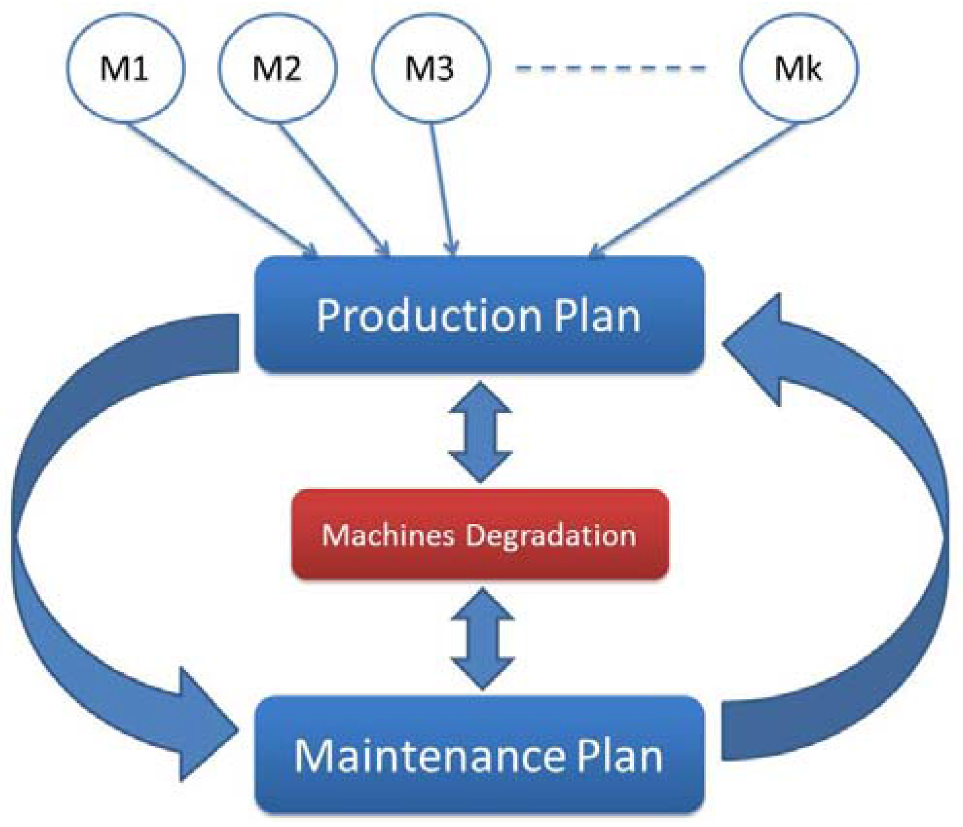
Figure 1 is illustrated in order to simplify understanding the case study.
3. Production and Maintenance Problem Formulation
In what follows, we develop a mathematical model expressing the total cost including leasing, manufacturing, inventory holding, and maintenance costs over the considered finite horizon H. We give at first the expressions of the different costs separately:
- Cost of leasing the machines
Leasing facility has the advantage of low costs comparing to purchasing equipment. Once the number of machines to be leased is established, the company has to pay the fees of leasing per production period as well as a fixed cost of administration settled by the lessor. The cost of leasing the machines for a period k is given by:
- Cost of installation/removal of the machines
Inspired from Holt et al. [22], where the authors considered a variable level of workforce, we can express the cost of setup and removal of machines as follows:
This equation includes the costs due to variation in the number of the machines required for period k (e.g,: costs of installation/ uninstallation, mobilization/demobilization). The constant term c4 describes the asymmetry in costs of adding and eliminating machines. As in HMMS model, we use here a quadratic formulation for the problem since it allows for a more realistic cost structure in the planning process as explained by Hax et al. [23].
- Manufacturing cost
where , and are binary variables expressed as follows:
- Inventory holding cost per period
We assume that the manufacturer should always maintain an optimal level for inventory as safety stock to hedge against shortages and which is equal to × , where are two constants chosen by manufacturer.
The inventory cost is calculated as below:
Otherwise, two cases may take place:
- -
- If × : the manufacturer should bear more costs due to over-stock (e.g., more space to be rented to hold this stock, more personnel costs, etc.)
- -
- If × : the manufacturer may pay costs of holding a stock that he is not really holding (e.g., rented space for stocking without using it, etc.)
- Total Maintenance cost
The global maintenance cost includes group preventive maintenance and corrective maintenance activities costs. It can be expressed as follows:
with
The average number of failures is given by the following expression:
where the failure rate in a period k for each machine is given by the following equation:
The objective function of the total cost for our production system can now be expressed as follows:
Subject to:
4. Optimization Approach
In order to find the different optimal values of the decision variables, i.e., number of group preventive maintenance actions over the horizon, number of machines to be leased and quantities to produce in order to satisfy the random demand, we use an algorithm based on branch and bound and random exploration methods combined with gravity center approach (GCA).
4.1. Random Exploration
This method consists in generating randomly a solution Si and then evaluating the objective function F considering solution Si. These two steps should be repeated until a fixed number of iterations is reached. We find few references in literature dealing with this method, which can be due to the randomness that characterizes it. This method has been criticized by specialists, it is worth mentioning that while dealing with big sized problems or those with multi-modal objective function, the random exploration may help to reduce the problem size before exploring it, using another method based on global or local neighborhoods and many specialists confirm this point.
Moreover, this method may be useful to have an idea about the “response surface” of the objective function and that can be achieved mainly by considering a three-dimensional representation. If the surface points out few irregularities, an extrapolation can be performed saying that the problem is not complex. But, if there are a lot of irregularities and with important amplitude, the problem is certainly considered as a complex one.
4.2. Branch and Bound
Branch and Bound is a method used to find the optimal solutions to problems, typically discrete problems. It is an algorithm that explores almost the entire space of candidate solutions, and throws out large parts of the search space by using previous estimates on the quantity being optimized. A branch-and-bound algorithm can be described as a tree search. At any node of the tree, the algorithm must make a finite decision and set one of the unbound variables. This method consists in two steps:
- Branching/Separation
This step consists in dividing the original problem into a number of sub-problems, which have each one its feasible solutions. So that, by resolving all these sub-problems and considering the best obtained solution, we are sure about resolving the initial problem. The set of solutions and the correspondent sub-problems have a natural hierarchy of a tree always called tree of research or tree of decision.
- Bounding/Evaluation
After constructing the tree of decision, the second step aims at selecting the leaf, which should be studied. Otherwise, this step consists in determining the optimum between the feasible solutions associated to a particular node or proving mathematically that this set of feasible solutions does not contain an interesting solution for the problem resolution. If such a node is identified in the tree, it is useless to perform the separation step on its solutions space.
4.3. Gravity Center Approach
In the literature, the GCA is frequently used in logistics systems in order to study the location selection of single distribution center [24,25]. It is used to minimize the sum of depot operating cost and routing costs [26].
We adopt this approach in the following part and apply it to our manufacturing system in order to find an optimal preventive maintenance plan. Our methodology consists of determining an optimal maintenance interval at which we can group several preventive maintenances so that . In order to find the value of , we use the following expression used to find the center-of-gravity of different points:
with is the weight factor assigned to each machine i and it corresponds in our case study to the average number of failures for each machine i; is the maintenance interval of each machine for an individual maintenance strategy; and is the distance (in time unit) between the group maintenance location (interval) and the individual maintenance location for each machine i. can be described as follows:
The choice of the average number of failures as the weight factor is justified by the fact that the degradation of each machine i is strongly correlated to its production rate (the quantity produced): more the machine works ( is important), more its degradation is high (average number of failures). So, it would be preferable to bring its maintenance closer to an optimal new date (or to bring it further otherwise). The expression of is as follows:
where the average number or failures for each machine i can be expressed as follows:
In order to find the optimal value of , we find at first a value using the following expression:
Once found, is replaced in Formula (11) in order to calculate . Then, a new value is found which will be replaced in the same formula in order to find another value , and so on, repeated until the two identical results show up within iterations. The value found corresponds to the optimal interval of group maintenance activity for the leased system.
Figure 2 describes the difference between individual and group preventive maintenance strategies for parallel leased machines system
4.4. Steps of the Resolution Method
- -
- Step 1: Generate randomly a solution Si for production plan: vector of number of machines to be leased and matrix and ;
- -
- Step 2: Calculate the total production cost and check if the service rate constraint is verified for the current solution;
- -
- Step 3: Evaluate the number of preventive maintenance activities for each machine for the current solution by minimizing the total maintenance cost;
- -
- Step 4: Group several maintenance activities using the center of gravity method and save the new interval of maintenance;
- -
- Step 5: Increment the time of repair to the minimal processing time of any machine for the current combination and update the new configuration of production and maintenance plans;
- Step 5.1: If the sum of processing times of machines in regular time is less than the maximal processing time for this equivalent work pattern, then browse through matrix Xn and find the minimum value;
- Step 5.2: If Step 5.1 is not verified and the sum of processing times of machines in overtime is less than the maximal processing time for this equivalent work pattern, then browse matrix Xs and find the minimum value;
- -
- Step 6: Repeat the same steps until founding the optimal solution Sn (return to Step 2);
- -
- Step 7: Save the optimal values of , , and ;
Figure 3 shows the algorithm of the resolution method.
4.5. Deterministic Transformation
Since our model is a stochastic one, to facilitate its resolution, we aim to transform it into a deterministic equivalent one. The certainty equivalent principle is the approach used among this transformation: thanks to the linearity of the model and assuming that the demand’s variation can be described by a Gaussian Process, we set the variables equal to their means ([27,28]). We remind that the inventory variable is strongly affected by the demand, which made it a stochastic variable. The different transformations are made in Appendix A and Appendix B.
Making all these deterministic transformations, we can now describe the model as follows:
Our constraints are as follows:
5. Numerical Example
In order to prove the efficiency of the proposed model, a numerical example is hereinafter studied. We put emphasis on the importance of group maintenance policy for a parallel leased machines system by comparing its results to an individual maintenance strategy. A case study of a company specialized in steel parts production using laser-machining tools is investigated. The laser machines are leased by the company in order to produce some products and satisfy some customers’ demand over the time horizon. The number of leased machines in each production period varies with the variation of customers’ demand. The processing time for each machine in regular time and overtime is variable. The failure rate of each machine depends strongly on the processing time (quantity produced) of each one. The study consists in minimizing the total production and maintenance costs expressed in monetary unit (mu) in order to find the optimal combination of number of machines to lease in each production period, the quantity to produce to satisfy the customers demand and the maintenance plan, consisting of the number of preventive maintenance activities to be performed, firstly in the case of an individual preventive maintenance policy and secondly for a group preventive strategy. As the firm receives a random demand, we vary hereinafter the dispersion of the ordered quantity of products in order to study its impact in the production and maintenance plans and to prove the efficiency of the developed group preventive maintenance policy. Two case studies are considered: in the first case, the random demand is characterized by a low standard deviation which gives nearly equal quantities produced by each machine in each production period. In the second case, we consider a random demand with a high standard deviation; the quantities of goods produced by each machine are then widely different from each other’s. The obtained results are shown in Table 1, Table 2, Table 3, Table 4, Table 5, Table 6, Table 7 and Table 8.
5.1. Case 1: Low Standard Deviation
We consider the following input data and present the corresponding results.
Temporal data: ∆k = 1; H = 20; ;
Cost coefficients: = 500; = 10; = 50; ; = 15; = 20; = 30; ;
Bounders: m = 4; M = 6; u = 40; ; ;
Service rate: β = 0.95 and initial inventory level: I0 =300;
Random Demand: = 25 and = 1000;
To compute the degradation function of each machine, we assume that the nominal degradation follows a Weibull distribution given by:
This quantity corresponds to a nominal processing rate when machines perform at their maximum level.
with: ; ;
5.1.1. Individual Maintenance Policy Results

Table 1.
Case 1: Production plan for individual maintenance policy.
| Period | dk | pk | Mk |
|---|---|---|---|
| Period 1 | 962 | 1000 | 5 |
| Period 2 | 1005 | 840 | 5 |
| Period 3 | 1001 | 920 | 6 |
| Period 4 | 1044 | 1040 | 6 |
| Period 5 | 994 | 1320 | 5 |
| Period 6 | 1022 | 760 | 5 |
| Period 7 | 935 | 920 | 6 |
| Period 8 | 998 | 1240 | 5 |
| Period 9 | 992 | 800 | 5 |
| Period 10 | 1004 | 1000 | 5 |
| Period 11 | 1013 | 1360 | 6 |
| Period 12 | 1007 | 1360 | 5 |
| Period 13 | 1010 | 1200 | 6 |
| Period 14 | 1026 | 840 | 6 |
| Period 15 | 1005 | 1240 | 5 |
| Period 16 | 1002 | 1520 | 6 |
| Period 17 | 1018 | 1200 | 6 |
| Period 18 | 986 | 1240 | 5 |
| Period 19 | 973 | 1400 | 5 |
| Period 20 | 989 | 1080 | 6 |
| Total cost | 1.1613 × 10⁷ mu | ||
Table 2.
Case 1: Maintenance plan for individual maintenance policy.
| Machine | Ni | Ti |
|---|---|---|
| Machine 1 | 4 | 5 |
| Machine 2 | 3 | 6.66 |
| Machine 3 | 3 | 6.66 |
| Machine 4 | 4 | 5 |
| Machine 5 | 3 | 6.66 |
| Machine 6 | 3 | 6.66 |
| Total cost | 5179.42 mu | |
5.1.2. Group Maintenance Policy Results
Table 3.
Case 1: Production plan for group maintenance policy.
| Period | dk | pk | Mk |
|---|---|---|---|
| Period 1 | 962 | 1000 | 5 |
| Period 2 | 1005 | 840 | 5 |
| Period 3 | 1001 | 920 | 6 |
| Period 4 | 1044 | 1040 | 6 |
| Period 5 | 994 | 1320 | 5 |
| Period 6 | 1022 | 780 | 5 |
| Period 7 | 935 | 920 | 6 |
| Period 8 | 998 | 1240 | 5 |
| Period 9 | 992 | 800 | 5 |
| Period 10 | 1004 | 1000 | 5 |
| Period 11 | 1013 | 1360 | 6 |
| Period 12 | 1007 | 1380 | 5 |
| Period 13 | 1010 | 1200 | 6 |
| Period 14 | 1026 | 840 | 6 |
| Period 15 | 1005 | 1240 | 5 |
| Period 16 | 1002 | 1520 | 6 |
| Period 17 | 1018 | 1200 | 6 |
| Period 18 | 986 | 1260 | 5 |
| Period 19 | 973 | 1400 | 5 |
| Period 20 | 989 | 1080 | 6 |
| Total cost | 1.1614 × 10⁷ mu | ||
Table 4.
Case 1: Maintenance plan for GPM policy.
| Total Maintenance Cost | ||
|---|---|---|
| 6.018 | 3 | 2636.7 mu |
5.1.3. Interpretations
Regarding the solution given in Table 1, we remark that the quantities produced by machines in each production period are nearly the same. This is due to the barely constant demand generated randomly by a relatively low standard deviation (). Given the correlation between failure rate and production rate for each machine, such a constant production plan leads to similar failure rates and automatically to similar number of failures; Table 2 shows clearly that the intervals of maintenance for machines are very close to each other in the case of an individual maintenance strategy (, , , , , ). When group maintenance policy is planned, we can remark through Table 3 that the production cost increases. This can be explained by the fact that an additional quantity of goods must be planned in order to hedge against shortages since all machines are maintained at the same interval. However, the maintenance cost thanks to group maintenance strategy decreases considerably, as shown in Table 4 (from 5179.42 mu to 2636.7 mu) and all machines are maintained at which proves the consistency of the proposed approach.
5.2. Case 2: High Standard Deviation
We consider the following input data and present the corresponding results.
Temporal data: ∆k = 1; H = 20; ;
Cost coefficients: = 500; = 10; = 50; ; = 15; = 20; = 30; ;
Bounders: m = 4; M = 6; u = 40; ; ;
Service rate: β = 0.95 and initial inventory level: I0 =300;
Random Demand: = 350 and = 1000;
5.2.1. Individual Maintenance Policy Results
Table 5.
Case 2: Production plan for individual maintenance policy.
| Period | dk | pk | Mk |
|---|---|---|---|
| Period 1 | 762 | 1840 | 6 |
| Period 2 | 762 | 960 | 5 |
| Period 3 | 1313 | 920 | 5 |
| Period 4 | 761 | 1400 | 5 |
| Period 5 | 431 | 1200 | 6 |
| Period 6 | 1095 | 960 | 5 |
| Period 7 | 1007 | 1080 | 5 |
| Period 8 | 925 | 1040 | 6 |
| Period 9 | 1006 | 960 | 5 |
| Period 10 | 1030 | 960 | 5 |
| Period 11 | 448 | 1400 | 6 |
| Period 12 | 897 | 1080 | 6 |
| Period 13 | 67 | 1360 | 6 |
| Period 14 | 682 | 2240 | 6 |
| Period 15 | 1358 | 1200 | 6 |
| Period 16 | 1125 | 1760 | 6 |
| Period 17 | 933 | 720 | 5 |
| Period 18 | 991 | 960 | 6 |
| Period 19 | 1211 | 1360 | 5 |
| Period 20 | 1111 | 1120 | 6 |
| Total cost | 2.8739 × 10⁷ mu | ||
Table 6.
Case 2: Maintenance plan for individual maintenance policy.
| Machine | Ni | Ti |
|---|---|---|
| Machine 1 | 3 | 6.66 |
| Machine 2 | 3 | 6.66 |
| Machine 3 | 5 | 4 |
| Machine 4 | 7 | 2.85 |
| Machine 5 | 3 | 6.66 |
| Machine 6 | 3 | 6.66 |
| Total cost | 5246.09 mu | |
5.2.2. Group Maintenance Policy Results
Table 7.
Case 2: Production plan for individual maintenance policy.
| Period | dk | pk | Mk |
|---|---|---|---|
| Period 1 | 762 | 1840 | 6 |
| Period 2 | 762 | 960 | 5 |
| Period 3 | 1313 | 920 | 5 |
| Period 4 | 761 | 1400 | 5 |
| Period 5 | 431 | 1200 | 6 |
| Period 6 | 1095 | 980 | 5 |
| Period 7 | 1007 | 1080 | 5 |
| Period 8 | 925 | 1040 | 6 |
| Period 9 | 1006 | 960 | 5 |
| Period 10 | 1030 | 960 | 5 |
| Period 11 | 448 | 1400 | 6 |
| Period 12 | 897 | 1100 | 6 |
| Period 13 | 67 | 1360 | 6 |
| Period 14 | 682 | 2240 | 6 |
| Period 15 | 1358 | 1200 | 6 |
| Period 16 | 1125 | 1760 | 6 |
| Period 17 | 933 | 720 | 5 |
| Period 18 | 991 | 980 | 6 |
| Period 19 | 1211 | 1360 | 5 |
| Period 20 | 1111 | 1120 | 6 |
| Total cost | 2.8741 × 10⁷ mu | ||
Table 8.
Case 2: Maintenance plan for individual maintenance policy.
| Total Maintenance Cost | ||
|---|---|---|
| 6.41 | 3 | 2593.3 mu |
5.2.3. Interpretations
Regarding the solution given in Table 5, we remark that the quantities produced by machines in each production period are widely different. This is due to the huge fluctuation of customers’ demand generated randomly by a relatively high standard deviation (). Such a difference in production rates leads to disparate failure rates and has a huge impact in number of failures; the difference between the intervals of maintenance for machines is relevant in the case of an individual maintenance strategy as shown in Table 6 (, and ). As well as in the first case, we can clearly remark through Table 7 and Table 8 that a group maintenance policy leads to an increase in production cost and a decrease in total maintenance cost (Total maintenance cost goes from 5246.09 mu to 2593.3 mu) which proves furthermore the consistency and robustness of the proposed approach.
5.3. Interpretation and Comments
Regarding the results shown in tables above, we can clearly remark that the group maintenance strategy is interesting for both cases (low and high standard deviation for the random demand) since it leads the firm to minimize the total costs of production and maintenance. The difference in maintenance costs between individual maintenance policy and group maintenance policy is more important in the second case. This can be explained by the fact that unlike the second case, the first case is characterized by a barely constant demand, the production rates of machines in each production period are then nearly similar which leads to very close failure rates. The intervals of maintenance are then close to each other and also close to the new interval of maintenance. Obviously, the total maintenance cost is minimized by adopting the group maintenance approach for both cases, but it is recommended to adopt it when production rates of machines are widely different. Concerning production costs, we can remark that in both cases, group preventive maintenance policy (GPM) leads to an increase in production costs. This can be explained by the fact that for the individual preventive maintenance policy (IPM), there is no need to interrupt production during maintenance activities since, even if few machines are under repair, other machines are still operating, unlike in the case of GPM where all machines are shut down for repair. The duration of preventive maintenance activity was taken into account in the production plan in order to satisfy customers’ demand and hedge against shortages. Table 9 recapitulates and shows a comparison of the performance of IPM and GPM strategies in term of costs for both cases.
6. Conclusions
Based on an industrial case study, this paper deals with a new developed approach in the frame of group preventive maintenance policy for parallel leased machines. Production and maintenance plans are studied taking into account new constraints related to leasing machines which have to work during regular and overtime work in order to satisfy a random demand over a finite time horizon and considering a given service rate.
Thus, to deal with this issue, and opting for a sequential resolution method, we start at first by proposing an approximate solution which minimizes the production costs under constraints related especially to service rate and equipment availability. Secondly, the obtained optimal production plan was considered as input data to perform the individual maintenance plan. To do this, we proposed an algorithm which allows organizing maintenance actions over the finite time horizon taking into account the degradation of each leased machine according to its production rate. A correlated group preventive maintenance policy based on the Center-of-Gravity approach is then developed and integrated to the algorithm in order to find a new optimal interval of group maintenance which allows the firm minimizing both maintenance and total costs. To further validate the model, a sensitivity analysis has been performed considering two case studies in which we vary the distribution of the random demand in order to study its impact in the developed approach.
Author Contributions
Tarek ASKRI and Zied HAJEJ conceived and designed the mathematical models; Tarek ASKRI developed the approaches and the algorithms; Zied HAJEJ and Nidhal REZG evaluated the results; Nidhal REZG supervised the work and Tarek ASKRI wrote the paper.
Conflicts of Interest
The authors declare no conflict of interest.
Used Notations
The following notations are used throughout the paper:
| Parameter | Explanation |
| H | Number of production periods |
| Δk | Duration of each production period (months) |
| dk | Random demand for period k (k = 1, 2, …, H); |
| Mean of the Gaussian demand during period k (k = 1, 2, …, H); | |
| Variance of the Gaussian demand | |
| Ik | Inventory at the end of period k (k = 1, 2, …, H) |
| β | Service level to be satisfied at each period |
| pik | Quantity produced by machine i (i = 1, …, Mt) in period k (k = 1, 2, …, H) |
| pk | Total production quantity during period k (k = 1, 2, …, H) |
| Failure rate of a machine i during a production period k | |
| Nominal failure rate for maximal production level | |
| Average number of failures of the system | |
| Average number of failures of a machine i | |
| Tr | Repair time (preventive maintenance) (hours) |
| Decision Variables | |
| Mk | Number of machines during period k (k = 1, 2, …, H) |
| Number of time units (hours) that machine i (i = 1, …, Mk) works during period k (as normal time) (k = 1, 2, …, H) | |
| Number of time units (hours) that machine i (i = 1, …, Mk) works during period k (as overtime) (k = 1, 2, …, H) | |
| Ni | Number of individual preventive maintenances to be performed in a machine i |
| N | Number of group preventive maintenance actions during time horizon |
| Ti | Interval between two successive individual preventive maintenances |
| Tn | Interval between two successive group preventive maintenances |
| Boundaries Variables | |
| M | Upper boundary of machines number |
| m | Lower boundary of machines number |
| u | Number of pieces that a machine can produce per time unit (hour); (the same for all machines) |
| Maximum of time units (hours) that a machine could be operated during a period as regular time | |
| Maximum of time units (hours) that a machine could be operated during a period as overtime | |
| Production Costs | |
| Average cost of leasing a machine | |
| Fixed costs of leasing (e.g,: administration costs) | |
| Cost of installation/removal of a machine from period k − 1 to period k | |
| Constant of asymmetry in costs | |
| Operating cost per overtime hour | |
| Operating cost per normal hour | |
| Cost to be paid to hold a produced unit in stock | |
| Optimal net stock | |
| Maintenance costs | |
| Total maintenance cost | |
| Unit preventive maintenance cost | |
| Unit corrective maintenance cost | |
Appendix A
Net Inventory Transformation
We recall that:
We have:
Since:
Thus, using the variance expression, we obtain:
Assuming that and using this equality and by iterations, we can easily proof that:
Since the variance expression of Ik can be written as follows:
So, we obtain:
On the other hand, we have
So,
And
Using both equalities above, we can conclude the following expected expression:
Also, we can write:
Regarding the two above equations, we obtain:
We assume that V(I0) = 0, therefore in the objective function we can make the following transformation:
Appendix B
Service rate Constraint Transformation
From the previous proof, the variance of inventory variable is defined by . This inventory variable depends linearly on the random demand variation. It is possible to consider the inventory variable as a random variable following a normal distribution defined by:
with is a standard Gaussian deviate.
Assuming that is the repartition function of this variable X.
is strictly increasing, indefinitely differentiable and therefore we conclude that is invertible:
References
- Mohamed-Salah, O.; Rezg, N.; Xie, X. Maintenance préventive et optimisation des flux d’un système de production. J. Eur. Syst. Autom. 2002, 36, 97–116. [Google Scholar]
- Chelbi, A.; Ait-Kadi, D. Analysis of a production/inventory system with randomly failing production unit submitted to regular preventive maintenance. Eur. J. Oper. Res. 2004, 156, 712–718. [Google Scholar] [CrossRef]
- Rezg, N.; Mati, Y.; Xie, X. Joint optimization of preventive maintenance and inventory control in a production line using simulation. Int. J. Prod. Res. 2004, 44, 2029–2046. [Google Scholar] [CrossRef]
- Dellagi, S.; Rezg, N.; Xie, X. Preventive maintenance of manufacturing systems under environmental constraints. Int. J. Prod. Res. 2007, 45, 1233. [Google Scholar] [CrossRef]
- Dahane, M.; Clementz, C.; Rezg, N. Effects of extension of subcontracting on a production system in a joint maintenance and production context. Comput. Ind. Eng. 2010, 58, 88–96. [Google Scholar] [CrossRef]
- Zhao, S.; Wang, L.; Zheng, Y. Integrating production planning and maintenance: An iterative method. Ind. Manag. Data Syst. 2014, 114, 162–182. [Google Scholar] [CrossRef]
- Li, F.; Ma, L.; Sun, Y.; Mathew, J. Group maintenance scheduling: A case study for a pipeline network. In Engineering Asset Management 2011: Proceedings of the Sixth Annual World Congress on Engineering Asset Management, Cincinnati, OH, USA, 3–5 October 2013; Springer: New York, NY, USA, 2013; pp. 163–177. [Google Scholar]
- Cui, W.W.; Lu, Z.; Pan, Z. Integrated production scheduling and maintenance policy for robustness in a single machine. Comput. Oper. Res. 2014, 47, 81–91. [Google Scholar] [CrossRef]
- Fakher, H.B.; Nourelfath, M.; Gendreau, M. Joint production-maintenance planning in an imperfect system with quality degradation. In Proceedings of the 6th IESM Conference, Seville, Spain, 21–23 October 2015. [Google Scholar]
- Yalaoui, A.; Chaabi, K.; Yalaoui, F. Integrated production planning and preventive maintenance in deteriorating production systems. Inf. Sci. 2014, 278, 841–861. [Google Scholar] [CrossRef]
- Hnaien, F.; Yalaoui, F.; Mhadhbi, A.; Nourelfath, M. A mixed-integer programming model for integrated production and maintenance. IFAC-PapersOnLine 2016, 49, 556–561. [Google Scholar] [CrossRef]
- Okumoto, K.; Elsayed, E.A. An Optimum Group Maintenance Policy. Nav. Res. Logist. Q. 1983, 30, 667–674. [Google Scholar] [CrossRef]
- Sheu, S.-H.; Jhang, J.-P. A generalized group maintenance policy. Eur. J. Oper. Res. 1996, 96, 232–247. [Google Scholar] [CrossRef]
- Koochaki, J.; Bokhorst, J.A.C.; Wortmann, H.; Klingenberg, W. Condition based maintenance in the context of opportunistic maintenance. Int. J. Prod. Res. 2012, 50, 6918–6929. [Google Scholar] [CrossRef]
- Yang, D.-L.; Cheng, T.C.E.; Yang, S.-J.; Hsu, C.-J. Unrelated parallel-machine scheduling with aging effects and multi-maintenance activities. Comput. Oper. Res. 2012, 39, 1458–1464. [Google Scholar] [CrossRef]
- Do, P.; Vu, H.C.; Barros, A.; Bérenguer, C. Maintenance grouping for multi-component systems with availability constraints and limited maintenance teams. Reliab. Eng. Syst. Saf. 2015, 142, 56–67. [Google Scholar] [CrossRef]
- Shafiee, M.; Finkelstein, M. An optimal age-based group maintenance policy for multi-unit degrading systems. Reliab. Eng. Syst. Saf. 2015, 134, 230–238. [Google Scholar] [CrossRef]
- Xiao, L.; Song, S.; Chen, X.; Coit, D.W. Joint optimization of production scheduling and machine group preventive maintenance. Reliab. Eng. Syst. Saf. 2016, 146, 68–78. [Google Scholar] [CrossRef]
- Renna, P. Influence of maintenance policies on multi-stage manufacturing systems in dynamic conditions. Int. J. Prod. Res. 2010, 50, 345–357. [Google Scholar] [CrossRef]
- Zhang, D.; Zhang, Y. Dynamic decision-making for reliability and maintenance analysis of manufacturing systems based on failure effects. Enterp. Inf. Syst. 2016, 1–15. [Google Scholar] [CrossRef]
- Hajej, Z.; Rezg, N.; Askri, T. A production planning optimization for multi parallel machine under withdrawal right. In Proceedings of the 6th International Conference on Industrial Engineering and Operations Management (IEOM), Dubai, United Arab Emirates, 3–5 March 2015; pp. 1–5. [Google Scholar]
- Holt, C.C.; Modigliani, F.; Muth, J.F.; Simon, H.A. Planning Production, Inventory and Work Force; Prentice-Hall: Englewood Cliffs, NJ, USA, 1960. [Google Scholar]
- Hax, A.C.; Candea, D. Production and Inventory Management; Prentice-Hall: Englewood Cliffs, NJ, USA, 1984. [Google Scholar]
- Chen, Z.; Wei, H. Study and Application of Center-of-Gravity on the Location Selection of Distribution Center. In Proceedings of the 2010 International Conference on Logistics Systems and Intelligent Management, Harbin, China, 9–10 January 2010; pp. 981–984. [Google Scholar]
- Watson-Gandy, C.D.T. A Note on the Centre of Gravity in Depot Location. Manag. Sci. 1972, 18, B478–B481. [Google Scholar] [CrossRef]
- Laporte, G.; Nobert, Y. An exact algorithm for minimizing routing and operating costs in depot location. Eur. J. Oper. Res. 1981, 6, 224–226. [Google Scholar] [CrossRef]
- Silva Filho, O. Linear quadratic gaussian probelm with constraints applied to aggregated production planning. In Proceedings of the 2001 American Control Conference, Arlington, VA, USA, 25–27 June 2001. [Google Scholar]
- Silva Filho, O.S.; Ventura, S.D. Optimal feedback control scheme helping managers to adjust aggregate industrial resources. Control Eng. Pract. 1999, 7, 555–563. [Google Scholar] [CrossRef]
Figure 1.
Problem Description.

Figure 2.
Comparison between IPM and GPM policies.
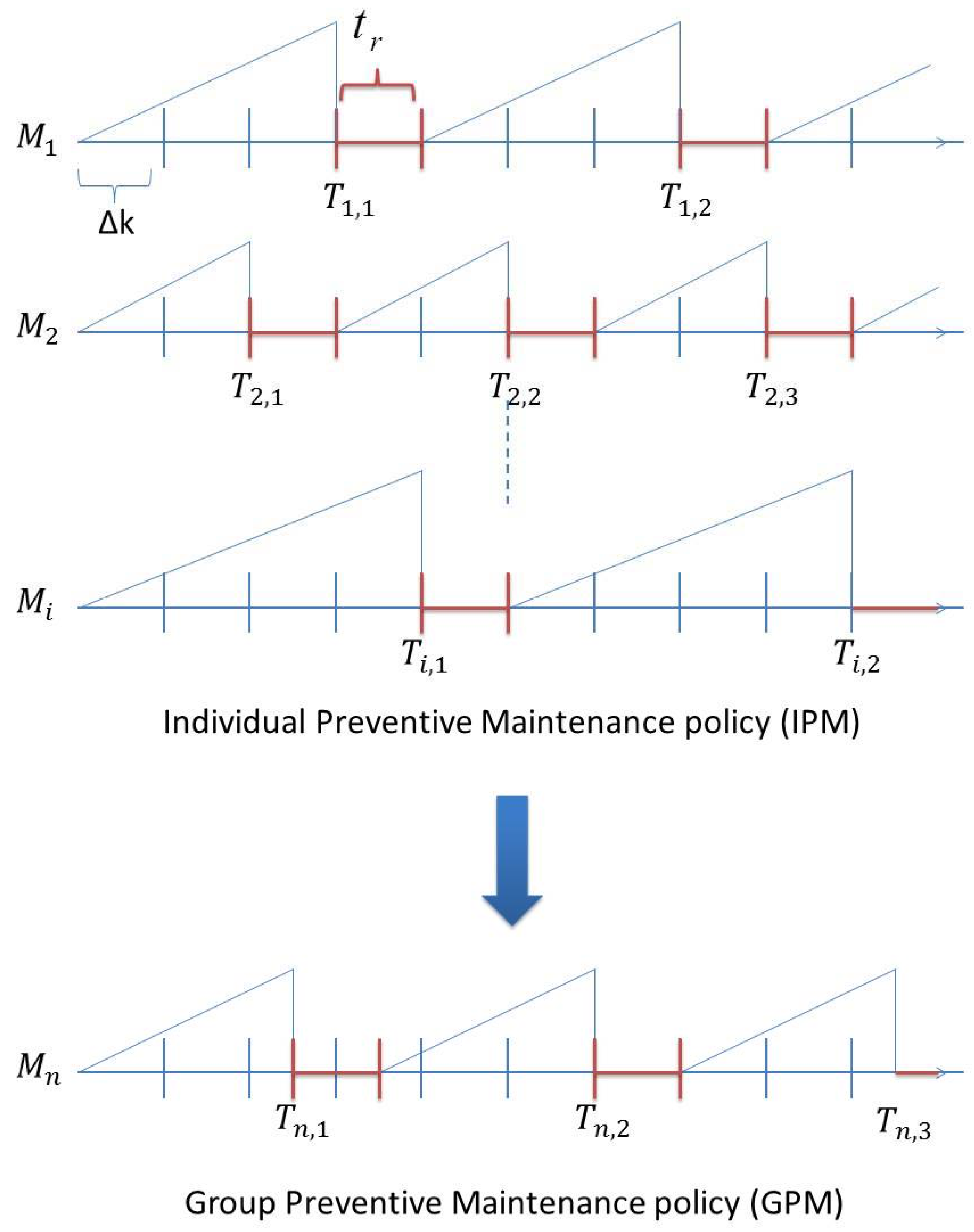
Figure 3.
Steps of the resolution approach.
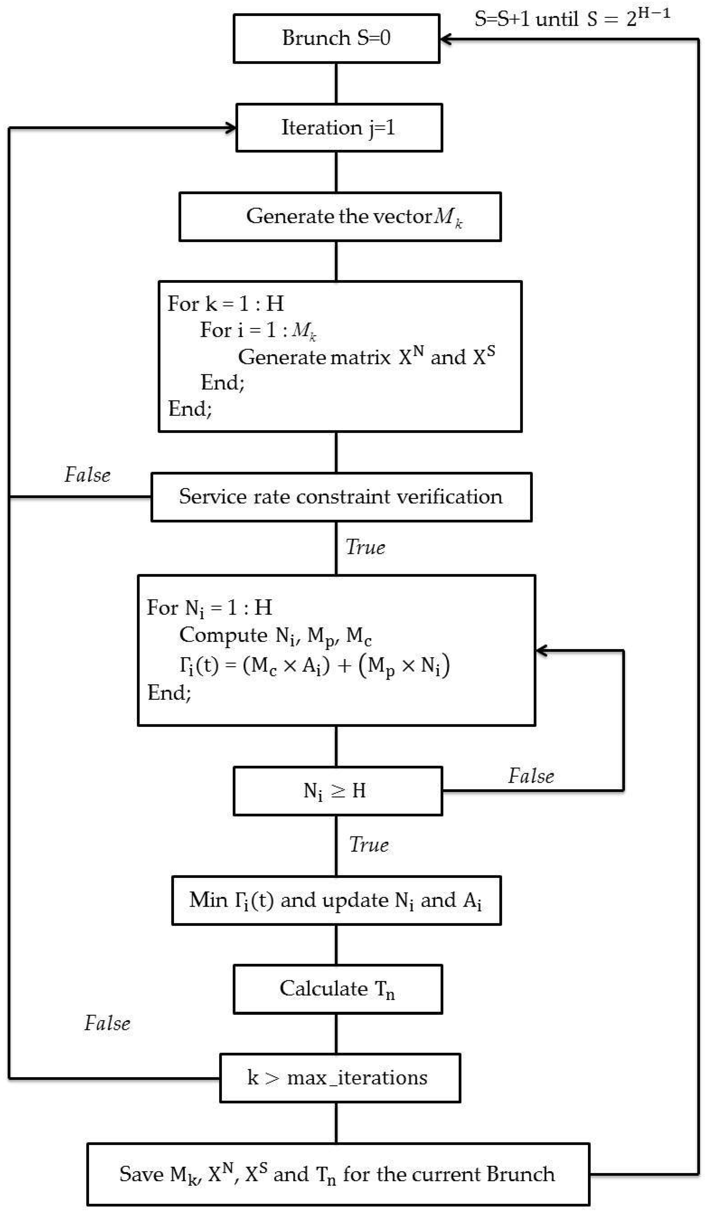
Table 9.
Comparison of the performance of the considered approaches for both cases.
| Case I | Case II | |
|---|---|---|
| Production Cost (IPM) | 1.1613 × 10⁷ mu | 2.8739 × 10⁷ mu |
| Production Cost (GPM) | 1.1614 × 10⁷ mu | 2.8741 × 10⁷ mu |
| Individual Maintenance Cost | 5179.42 mu | 5246.09 mu |
| Group Maintenance Cost | 2636.7 mu | 2593.3 mu |
| Total Cost for IPM | 1.16181 × 10⁷ mu | 2.87441 × 10⁷ mu |
| Total Cost for GPM | 1.16166 × 10⁷ mu | 2.87435 × 10⁷ mu |
© 2017 by the authors. Licensee MDPI, Basel, Switzerland. This article is an open access article distributed under the terms and conditions of the Creative Commons Attribution (CC BY) license (http://creativecommons.org/licenses/by/4.0/).
Share and Cite
MDPI and ACS Style
ASKRI, T.; HAJEJ, Z.; REZG, N. Jointly Production and Correlated Maintenance Optimization for Parallel Leased Machines. Appl. Sci. 2017, 7, 461. https://doi.org/10.3390/app7050461
AMA Style
ASKRI T, HAJEJ Z, REZG N. Jointly Production and Correlated Maintenance Optimization for Parallel Leased Machines. Applied Sciences. 2017; 7(5):461. https://doi.org/10.3390/app7050461
Chicago/Turabian StyleASKRI, Tarek, Zied HAJEJ, and Nidhal REZG. 2017. "Jointly Production and Correlated Maintenance Optimization for Parallel Leased Machines" Applied Sciences 7, no. 5: 461. https://doi.org/10.3390/app7050461
Note that from the first issue of 2016, this journal uses article numbers instead of page numbers. See further details here.