
Subsidence Evolution of the Leizhou Peninsula, China, Based on InSAR Observation from 1992 to 2010


1
School of Geosciences and Info-Physics, Central South University, Changsha 410083, China
2
*Correspondence: [email protected]
*
Author to whom correspondence should be addressed.
Appl. Sci. 2017, 7(5), 466; https://doi.org/10.3390/app7050466
Submission received: 2 March 2017
/
Revised: 21 April 2017
/
Accepted: 26 April 2017
/
Published: 29 April 2017
Abstract
:Over the past two decades, the Leizhou Peninsula has suffered from many geological hazards and great property losses caused by land subsidence. However, the absence of a deformation map of the whole peninsula has impeded the government in making the necessary decisions concerning hazard prevention and mitigation. This study aims to provide the evolution of land deformation (subsidence and uplift) in the whole peninsula from 1992 to 2010. A modified stacking procedure is proposed to map the surface deformation with JERS, ENVISAT, and ALOS1 images. The map shows that the land subsidence mainly occurs along the coastline with a maximum velocity of 32 mm/year and in a wide range of inland arable lands with a velocity between 10 and 19 mm/year. Our study suggests that there is a direct correlation between the subsidence and the surface geology. Besides, the observed subsidence in urban areas, caused by groundwater overexploitation for domestic and industrial use, is moving from urban areas to suburban areas. In nonurban areas, groundwater extraction for aquaculture and arable land irrigation are the main reason for land subsidence, which accelerates saltwater intrusion and coastline erosion if regular surface deformation measurements and appropriate management measures are not taken.
1. Introduction
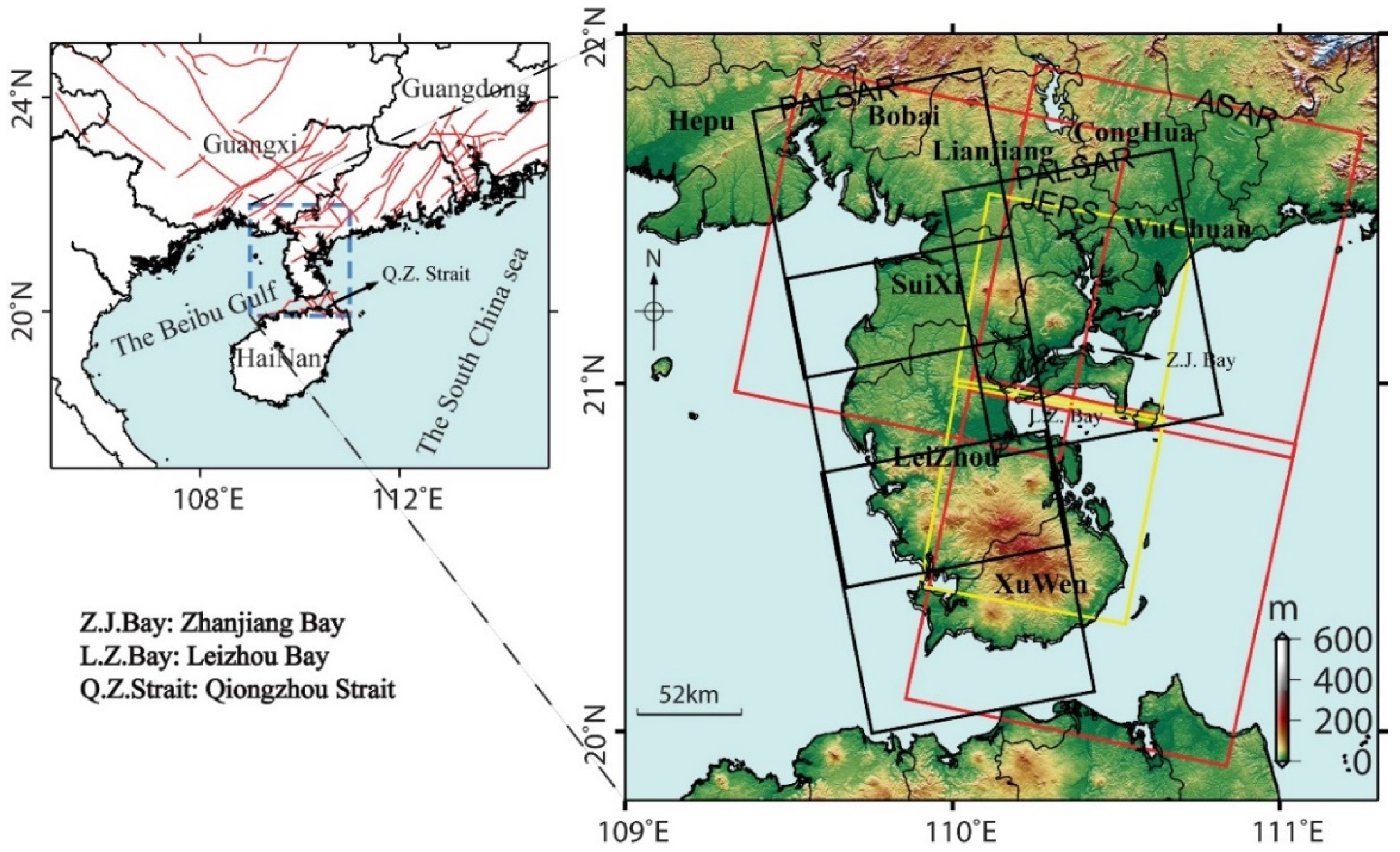
The Leizhou Peninsula (LZP), one of the three largest peninsulas in China, is located in the southwest of Guangdong province, China, covering an area of 8500 km² [1] (see Figure 1). It plays an important role in the economic development of Guangdong province with its considerable agriculture contributions. However, over the past two decades the fast growing economy has accelerated groundwater over-pumping, causing large scale land subsidence and other geological hazards. Until 2001, the subsidence area in Zhanjiang city reached 220 km², with the maximum cumulative subsidence up to 17.9 cm [2]. Subsidence induced geological hazards have resulted in substantial property damage every year. For example, in 2006 only, the loss in Zhanjiang city was greater than 90 million RMB [3]. However, large-scale land subsidence measurement is still scarce in the LZP apart from a few leveling measurements carried out in the urban area of Zhanjiang city in 1984, 1989, 1999, and 2001, whose results indicated that the surface subsidence increased by >10 mm/year [2,4]. A surface deformation map presenting the temporal-spatial pattern of land subsidence of the whole peninsula is urgently needed to help the government make the right decisions in geological disaster prevention and mitigation, as well as to understand the mechanism of land subsidence caused by over-pumping groundwater.
Interferometric Synthetic Aperture Radar (InSAR), a satellite based technique, offers high precision (cm even to mm), high spatial resolution, and wide coverage measurements of surface deformation, reducing the use of in-situ traditional techniques [5,6]. Furthermore, with the development of the SAR satellite missions, more and more newly acquired TerraSAR, COSMO-SkyMed, Sentinel-1, ALOS-2 and archived SAR data (ERS1/2, JERS-1, ENVISAT, ALOS1) can be used to analyze the spatial-temporal characteristics of large area surface deformation with the temporal InSAR technique [7]. Therefore, the InSAR technique can serve as a good option in mapping the surface deformation of a large-scale area. Actually, it has been widely used and its superiorities shown in detecting time-series surface deformation over many peninsulas and delta areas, such as the Mexico City [8], Shanghai [9], and Indonesia [10]. Traditional temporal InSAR methods, such as Persistent Scatterer Interferometry (PS-InSAR), IPTA (Interferometric Point Target Analysis), and Small Baseline Subset (SBAS-InSAR) have been applied in detecting surface deformation, but they need abundant SAR images in data processing [11,12,13]. As the datasets are very limited in our study area, we used a modified stacking method to measure the surface deformation evolution over the whole LZP with three kinds of SAR images (JERS, ENVISAT and ALOS1) acquired from 1992 to 2010. Based on those results, the reasons and mechanisms of land subsidence can be explained and are investigated in this study.
Here, we map the surface deformation of three different sensor platforms and illustrate the spatial-temporal evolution patterns in urban and agriculture areas. Based on the surface hydrogeological and land use, we analyze the reason for land subsidence. The consequences and implications of our land subsidence measurement are discussed in the last section.
2. Hydrogeological Setting
The study area is the most southerly tip of China, with Qiongzhou Strait to the south, separating the peninsula from Hainan Island. The elevation of this area ranges from a few meters along the coast to 275 m in the south of this peninsula, see Figure 1. The Suixi Fault borders the area in the north, see Figure 2a. Terranes of Cambrian age and Cretaceous age constitute the basement rocks of this peninsula. Tertiary semi-consolidated sandy clay and Quaternary unconsolidated sediments, such as alluvial and lacustrine, overlie the basement rocks. The unconsolidated sediments include (1) Zhanjiang Group of Lower Pleistocene age with an upper layer of clay and a lower layer of scattered lenses of clay and coarse sand with gravel (Qlz), (2) Beihai group of middle Pleistocene age with a surface layer of clayey sand and a lower layer of sand with gravel (Q2b), (3) Recent sediments of Quaternary age with silty sand and clayey coarse sand (Q4), (4) basalt of Himalayan Period occurs in Quaternary sediments (β) with lots of dead craters [14], as shown in Figure 2a. In order to obtain the relationship between land subsidence and unconsolidated sediments, the soft soil thickness derived from 22 boreholes with an ordinary Kriging interpolation were generated (see Figure 2b). The soft soil thickness for each borehole was calculated as the total thickness of silt, sand and gray-clay which overlaid the upper layer of gravels above the basement [15,16].
The aquifer system in this peninsula can be grouped into three subsystems, shallow aquifer, middle aquifer, and deep aquifer [4,14]. The shallow aquifer is an unconfined aquifer and mainly located at Q2b, Qlz, and Q4. Its maximum depth is 30 m. The middle aquifer occurs approximately from 30 to 200 m. The depth of the deep aquifer ranges from 200 to 500 m. The latter two kinds are confined aquifers, extending laterally to the coast. The recharge of the unconfined aquifer is mainly derived from precipitation with an annual rainfall of 1500 mm [4,14], and infiltration of canal and reservoir. Besides the leakage recharge of confined aquifer, the deep aquifer can also be recharged directly from unconfined aquifer [14]. This is because the wide range distribution of β and dead craters (3694 km2), as shown in Figure 2a, has a high water content up to a depth of 310 m, deep enough to connect to the deep aquifer [14]. The discharge of the aquifer system is of two types, one is subterranean discharge into the sea and the other is artificial pumping. Groundwater is extracted from aquifers through production wells for water supply, such as agricultural irrigation, together with industrial and residential water [2,4]. In addition, we also collected the land use map, see Figure 2c, to better interpret the relationship between land subsidence and land use in the following discussion [3].
3. Data Coverage and Method
3.1. Data Coverage and InSAR Processing
Here we use the SAR data from the L-band JERS, ALOS, and the C-band ENVISAT satellites to map the line-of-sight (LOS) surface deformation. There are three kinds of SAR images, including 42 ALOS1 images acquired from two parallel ascending-orbit tracks from December 2006 to July 2010, 22 JERS images acquired from October1992 to September 1998, and 23 ENVISAT images acquired from October 2003 to May 2007 (See Figure 1 and Table S1–S3). Those InSAR datasets provide deformation of a 200 × 100 km area covering the whole peninsula (see Figure 1). Detailed SAR data information is shown in Table S1–S3.
These SAR data are processed by the conventional two-pass differential interferometry methods of GAMMA software package [17]. We applied a multilook operation of 6 × 16 pixels for the ALOS1, JERS data and 4 × 20 for the ENVISAT data in the range and azimuth directions to reduce the phase noise as well as calculation burdens before the phase unwrapping. Using the 90-m resolution SRTM v4.2 digital elevation model, we removed the phase relating to topography. The refined ESA VOR orbits were used to remove the phase ramps for the ENVISAT acquisitions. However, there was no precise orbit for the JERS or ALOS1 data. So we adopted a refined method based on fringe frequency to correct the phase ramp in differential interferograms [18]. Before phase unwrapping, a modified Goldstein filter was used to reduce noise phases [19] and a manual mask applied to eliminate its impact on phase unwrapping from some low coherence areas such as isolated islands and sea areas. In some studies, ionospheric disturbance error of SAR interferogram also needed to be considered [20,21], but we did not find any SAR images contaminated by ionospheric disturbances in this study. Finally, we used minimum cost flow algorithm to unwrap pixels whose coherence value was over a threshold (0.7).
Combination of ascending and descending modes can be used to separate vertical and horizontal ground motions. However, here only the ascending ALOS1 or the descending JERS and ENVISAT acquisitions can be used in every time span. Thus vertical and horizontal components of the deformation are impossible to be retrieved independently [22]. Our results show that most ground displacement rates are <30 mm/year and the vertical subsidence is the main deformation component [23]. Thus, we assumed that the horizontal ground displacement is negligible and projected the results in LOS direction to vertical direction by dividing by the cosine of the incidence angles of each platform.
3.2. Modified Stacking Method
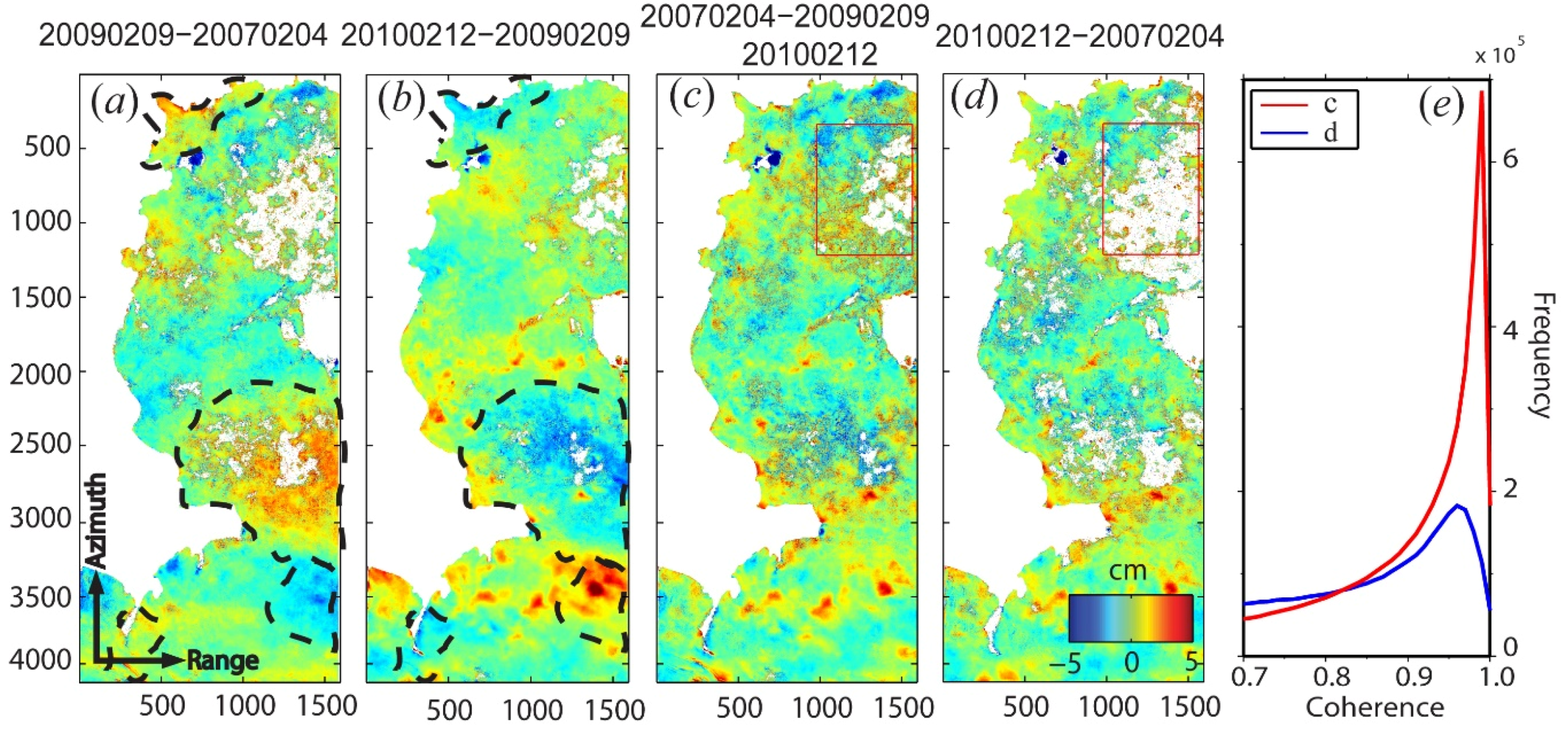
The stacking technique can mitigate atmospheric delays and measure uniform surface deformation by averaging data with multiple interferograms [24]. However, there are very limited images for every frame (≤11 images) in this study (see Table S1–S3). What is worse, lots of SAR images have significant atmospheric delays due to strong evaporation in the LZP, especially in summer. For example, four of the 10 observations have serious atmospheric effects for track466/frame400 of ALOS1 acquisitions (see Figure S1 and Table S1). In order to make full use of all available images in the stacking process, we firstly obtained unwrapped differential interferogram pairs frame by frame. Secondly, we manually identified the images with serious atmospheric delays and then used pair wise logic instead of the traditional stacking method which combine pairs in a chronological order. It means every identified image should be treated as master and slave in turn for the final differential pairs used, see Figure S2. This process can not only reduce the atmospheric effect but also strengthen the effective value decided by mean coherence in the combined interferogram. Figure 3 shows the differential interferogram of ALOS1 before and after using this strategy and the coherence histograms of Figure 3c,d are also calculated in Figure 3e. We can find that the mean coherence of stacking in Figure 3c is obviously better than that of Figure 2d obtained by direct interferometry (see Figure 3e). The atmosphere effects of image 20090209 represented by black dashed lines in Figure 3a,b are also mitigated in Figure 3c by the combination of Figure 3a,b. Moreover, the cumulative perpendicular baseline of each frame should be close to zero to reduce topography error in the final stacking results. Finally, we calculated the linear displacement rate with the ratio between the cumulative unwrapped phase and cumulative time. It should be noted that the method above is different from the one proposed by Biggs [25], in which every SAR acquisition can be used only twice through the chain stacking. We used SAR images with atmosphere contaminated twice only if the frequency of master and slave were the same. In addition, to analyze the development of subsidence in urban areas more scientifically, we also used a traditional SBAS-InSAR to calculate the deformation time-series in the capital city of LZP, Zhanjiang city [12].
3.3. Uncertainty Estimation
The cumulative phase is the sum of phases, including surface deformation , topography errors , atmospheric delays , satellite orbit errors , and thermal noise in the stacking process:
where is the unwrapped phase, K is the number of differential interferograms, and are the time span and perpendicular baseline of one interferogram, is the wavelength of SAR images, is the distance between satellite and ground and is the residue DEM error. In order to obtain the precise surface deformation, the potential spurious phase, i.e., orbital errors, topographic errors, and atmospheric delays, should be taken into account and minimized. The orbital error can be corrected by a 2-D linear or quadratic model in unwrapped interferograms [15] The atmospheric delays relating to topography can be neglected in this study due to the flat terrain, and the variance of neutral atmospheric delay has been mitigated by our modified stacking method. The topographic error also can be neglected here because the cumulative perpendicular baseline is close to 0 m [26], which can cause an error of 0.6 mm, 1.5 mm, and 3.5 mm with a 5 m DEM error for JERS, ENVISAT and ALOS1 respectively. We used several reference points to calibrate the results of three different platforms, assuming these points are stable with respect to the main movement areas. So we obtained the mean velocity () after considering the source errors listed above.
We calculated the variances of residual error in each selected interferogram and these results (up to 99, 183 and 140 mm² for ENVISAT, JERS and ALOS1) indicated that the atmospheric delay is sensitive in this study (see Figure S3). So we adopted a 1-D exponential covariance function to estimate the uncertainty of mean velocity [27], where is the variance, is the covariance, is the distance between pixels, and is a variable window size of each acquisition named e-folding wavelength. Figure 4 shows the 1-D covariance function of deformation velocity in three different sensors and their variance for JERS, ENVISAT, and ALOS1 are 3.0, 5.1, and 4.1 mm²/year² with the e-folding wavelengths as 2.0, 2.5, and 8.8 km respectively. Furthermore, we also utilized the residual error between the estimated velocity and the single interferograms to estimate velocity uncertainty and found that both methods gave very similar results. So the uncertainty we estimated in this study is considered to be reliable.
4. Results: Spatial—Temporal Evolution of Subsidence
4.1. Rates of Land Subsidence
The average vertical velocity map of the LZP was generated by the processes described in Section 3 with three kinds of SAR images acquired from 1992 to 2010. They are shown in Figure 5 with the order of their acquisition times. Figure 5a shows the velocity map of JERS. The main subsidence areas distribute along the coastline (the black dashed elongated lines). The peak land subsidence occurred in the southeast of Zhanjiang with a maximum velocity 26 mm/year. In urban areas the land subsidence occurred mainly in Zhanjiang city, with a velocity of 6–15 mm/year. Figure 5b is the velocity map of ENVISAT. Compared with the JERS data, the ENVISAT data has a much larger coverage but with comparatively poorer coherence due to the serious temporal decorrelation of the C-band satellite. There are three obvious subsidence areas shown in Figure 5b, such as the Zhanjiang city represented by red dashed rectangle, and two insets named ‘Nansan Island’ and ‘ZhaoZiLin’. The maximum subsidence rate (19 mm/year) appears in the coastal areas of Nansan Island. In addition to the land subsidence, there are also 1 to 2 mm/year uplifts in the southwest of the LZP. For the land subsidence from 2006 to 2010, we collected the ALOS1 images to map. As shown in Figure 5c, the main subsidence zones also distribute along the coastline (about 19 mm/year) defined by a black dashed line. Another feature of the subsidence is its discrete distribution in agricultural areas, see Figure 2c, such as farmlands in Leizhou and Suixi. Land uplift was observed in the southwest of the peninsula ranging from 1–3 mm/year, in accordance with results of ENVISAT data.
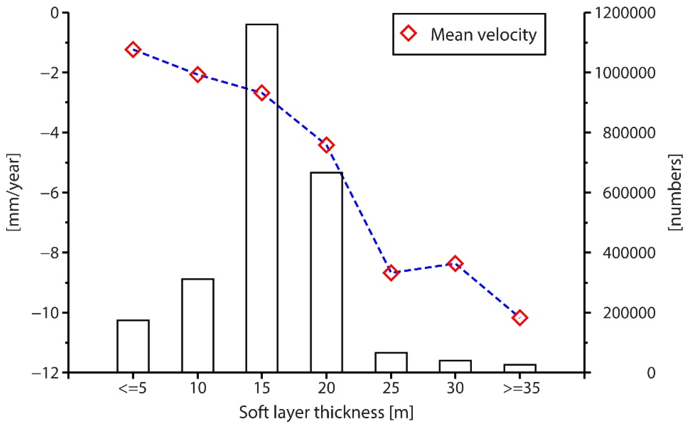
Based on the results in Figure 5, we can conclude that the major area of the LZP was stable during the period from 1992 to 2010, in spite of a small scale land subsidence in the urban and agricultural areas along the coastline. The subsidence in agricultural areas was moderate with a rate of ~19 mm/year. Furthermore, the subsidence area was spreading instead of being still during the image coverage time. For example, the subsidence center in the overlapped coverage area of JERS and ALOS1 was moving from the northeast of Xuwen to the junction areas of Leizhou and Xuwen. Also, the subsidence rate and range in urban areas were changing. This is further discussed in Section 4.2. The subsidence in coastal areas, increased both in rate and range, especially the area marked with black dashed lines (from 8–24 to 12–32 mm/year) in Figure 4a,c. This subsidence area is general consistent with that of the compressible deposit (Q4) distribution in Figure 2a. In order to quantitatively analyze the relationship between the depth of compressible sediments and land subsidence [28], we generated the distribution of recent soft soil thickness of the Holocene age with 22 boreholes by the method of [29], see Figure 2b. The statistical results of mean subsidence rate and pixel numbers of ALOS1 are shown in Figure 6 due to a more complete coverage compared with the other two satellites. We can see that the majority of the area is underlain by soft-soil thicknesses of 15–20 m, and the mean vertical velocity is growing with the increase of thickness, which agrees with the results of [30], i.e., maximum average deformation velocities are found on the thickest soft soils (>35 m), conversely, the mean velocity values calculated for the thinnest soft soils are satisfactorily within the precision range. The relationship between these two factors can help to interpret the mechanism of land subsidence.
4.2. Land Subsidence in the Urban Areas
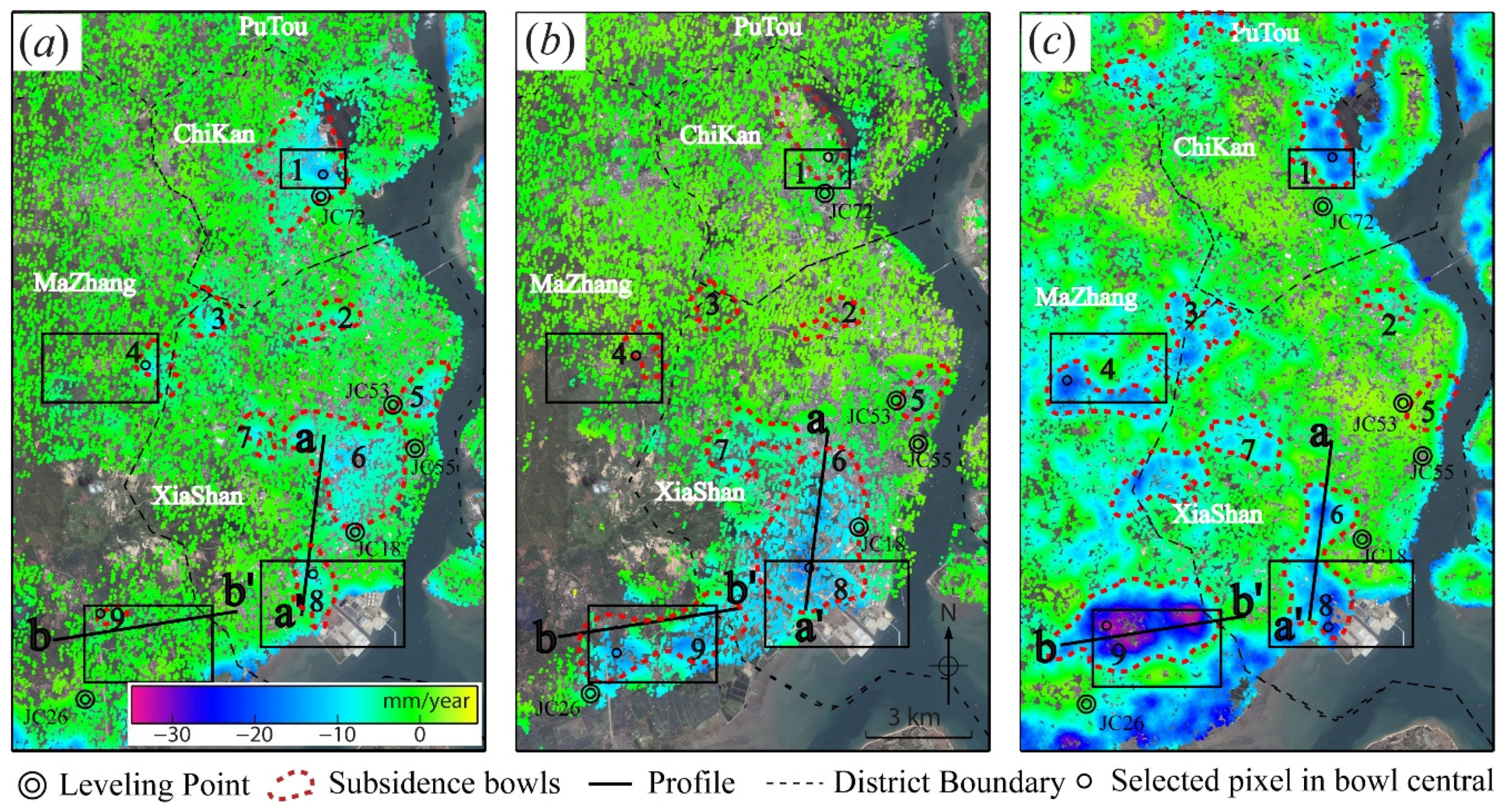
Zhanjiang is the largest city, the political and economic center of the LZP, with a population of 7.45 million until 2009. It has a long history of land subsidence, but only a few leveling measurements in the LZP from 1984 to 2001, which can help validate the InSAR measurement. Hence, we selected the area (latitude: 21.105°–21.330°, longitude: 110.281°–110.435°) with historic leveling measurements as the experiment area. The surface deformation of the chosen area is shown in Figure 7a–c. We chose nine representative subsidence bowls with a segmentation based on a threshold of mean velocity (0.9 mm/year), marked by red dashed lines in Figure 7, to demonstrate the spatial-temporal features of land subsidence. The land use of this city is showed by the inset in Figure 2c, where we can see that six bowls (bowl 1, 2, 5, 6, 7, and 8) are in the urban areas, and two bowls (bowl 3 and 4) are in the nearby agricultural area of Xiashan and Mazhang. Bowl 9 appeared in the suburb area. The subsidence areas of these nine bowls are calculated and shown in Table 1.
In addition to the average subsidence rate, we used SBAS-InSAR to generate the deformation time-series of these bowls. Four bowls with large subsidence rates, i.e., bowls 1, 4, 8, and 9, were selected to analyze the development of subsidence in the city, see Figure 8. Pixels located at or near the central of the bowl observed by each satellite were selected and plotted in Figure 7. In urban areas, such as bowl 1 and bowl 8, the deformation time-series approximates to linear, as observed in other areas [10]. The continual groundwater extraction will change the stress between confined aquifers and lead to the compaction of the compressible sediments, resulting finally in the land subsidence. However, the magnitudes of subsidence rate in these two bowls are different. Bowl 1 experienced two major changes, the subsidence rate first slowed down from 13 (Figure 8e) to 4 mm/year (Figure 8i) and then increased from 4 (Figure 8e) to 29 mm/year (Figure 8m), whereas bowl 8 increased during the periods (Figure 8g,k,o). Unlike the results of bowls 1 and 8, the subsidence of bowl 9 is complicated. In the first stage (Figure 8h), the deformation time-series trend is nonlinear, which is mainly caused by the seasonal groundwater pumping for irrigation or aquaculture along the coastline. For example, the uplift trends occur at summer (May 1995, July 1995, and August 1998) while the fall trends occur at spring (February 1997 and March 1998). The fall trends occurring at non-irrigation periods in this case may be caused by the delay from aquifer compaction to deformation. During the second stage (Figure 8l,p), the deformation time-series is close to linear. The main reason for this phenomenon is the exploitation of groundwater from the deep aquifer of the new waterworks named Lindong from 1999 [31], aiming to mitigate the over-pumping groundwater in urban areas. More details about bowl 9 are depicted by the profile bb' in Figure 9b showing the continued development of subsidence rates. Similarly, bowl 4 in the agricultural area experienced a nonlinear deformation. More importantly, the periodic deformation time-series of Figure 8f,j,n are observed, indicating the seasonal groundwater pumping for irrigation.
We also calculated the spatial-temporal evolution of land subsidence area showed in Table 1. Five bowls (Bowl 1, 2, 3, 4, and 5) of ENVISAT data are excluded due to their unclear boundaries. The subsidence area of bowls decreased with time in the urban area, for instance it decreased from 3.3 to 3.0 km² in bowl 1, from 1.9 to 0.8 km² in bowl 2, from 10.8 to 6.1 km² in the new bowl merged from bowl 6 and bowl 8. Conversely, in suburb and agricultural areas, the subsidence area increased continuously: from 0.9 to 4.3 and then to 12.2 km² in bowl 9, from 1.8 to 4.8 km² in bowl 3 and from 1.6 to 6.1 km² in bowl 4 (see Table 1). In order to analyze the spatial evolution of bowl 6 and bowl 8, another profile aa’ is plotted in Figure 9. We can see that the two separated bowls (red line in Figure 9a) merged into one bowl (green line in Figure 9a), and then became two connected bowls (blue line in Figure 9a) from a to a’, which can also be visually observed in Figure 7a–c. In addition to the subsidence area, the central bowl selected for bowls 1, 4, 8, and 9 aforementioned is regarded as the movement indication in this study. The results are shown in Figure 8a–d with red arrows, we can see that the surface subsidence extends from urban areas to suburban and agricultural areas.
It is known that subsidence in Zhanjiang city is the result of over-extraction of groundwater for domestic and industrial use [4,32]. Groundwater exploitation from middle and deep aquifers started in the1980s and accelerated in the 1990s with the development of the economy and urbanization. However, as our InSAR measurements suggest from 1992 to 2010 the subsidence rate decreased after the government prohibited pumping groundwater in the urban areas [32] (see Figure 7). Meanwhile, the subsidence rate started increasing in the suburban areas as the groundwater was extracted to supply the growing population and expanding industries in the urban areas accompanied by the moving of the waterworks. Besides, we take three small cities of the LZP into measurement, Leizhou city, Xuwen County, and Suixi County. Unlike Zhanjiang city, the subsidence in these cities is comparatively small with the average subsidence rate 0.6, 0.7, and 1.5 mm/year, respectively.
4.3. Land Subsidence in Agriculture Areas
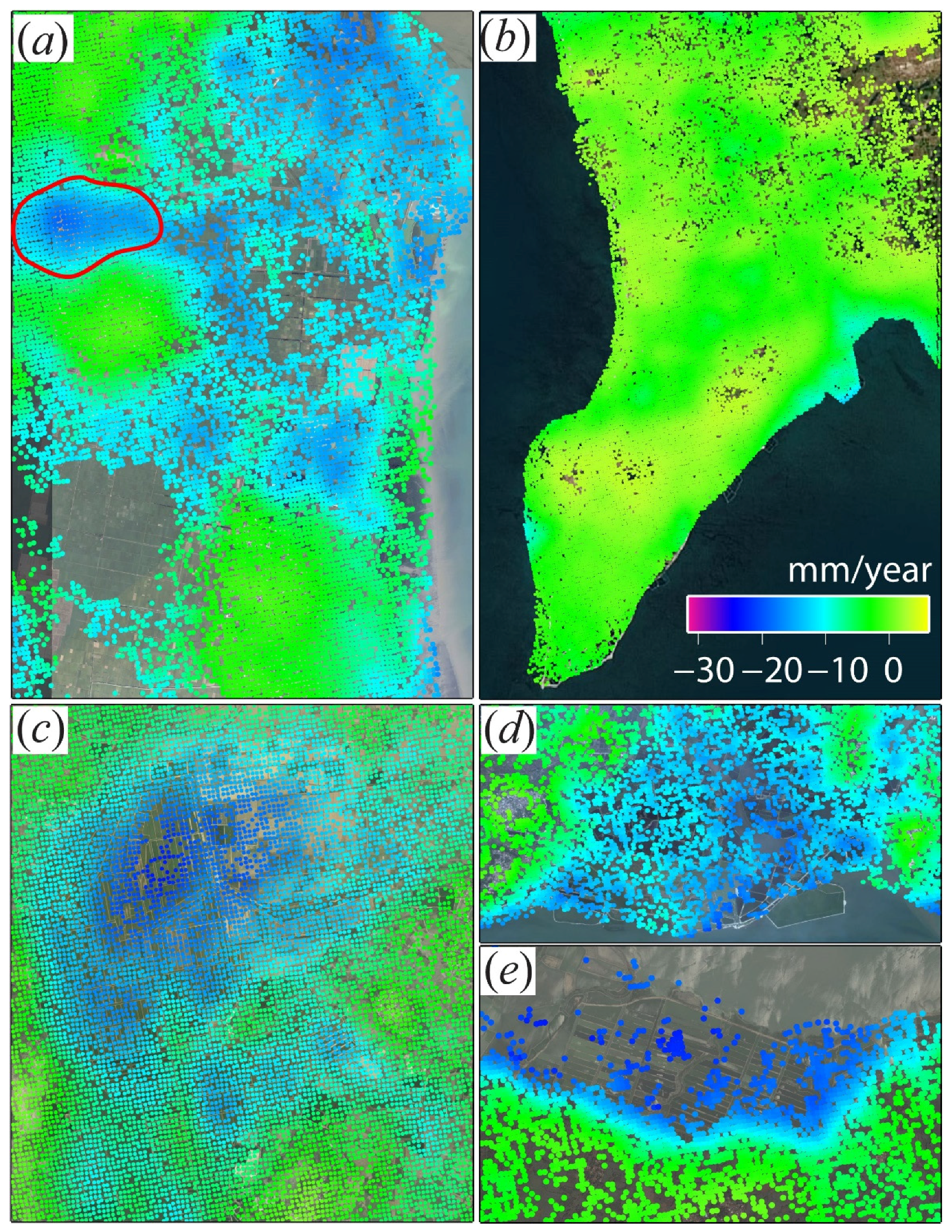
Besides urban areas, there is also some subsidence in agricultural areas caused by natural and anthropogenic processes. Here we only analyze the result of ALOS1 data because of the decorrelation and uncompleted coverage of ENVISAT and JERS data in those areas. From Figure 5c, we find that: (1) there is a wide range of discrete subsidence in the arable land with the rate of 10–19 mm/year, such as the junction area between Xuwen and Leizhou, the southwest of Leizhou; (2) rapid subsidence occurred along the coastline as shown by the black dashed elongated circles. The peak maximum subsidence in this area is up to 32 mm/year. In order to get more details, we chose five representative regions denoted by red rectangles (A–E) in Figure 5c to analyze the characteristics and causes of subsidence (see Figure 10).
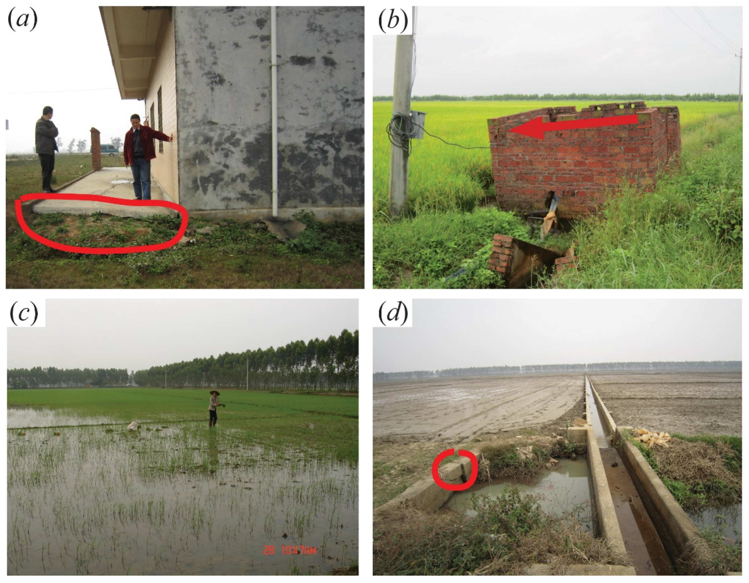
Subsiding areas shown in Figure 10a are farmlands characterized with highly compressible deposits, consisted of clay, silt, and silty sand (see Figure 2a), which is vulnerable to land subsidence due to sediment loading [8,33,34]. Shallow aquifers are the main supplier of these agricultural areas, which can be recharged seasonally from surface runoff, such as reservoirs and canals. However, during the observation period, the LZP experienced lots of droughts, resulting in the continuous declining of the shallow aquifers’ level [35]. Moreover, unguided drilling, such as mixed exploitation of water from shallow- and deep-aquifers [35], and illegal drilling both accelerated the shrinking of groundwater level and caused a wide range of land subsidence. The bowl in Figure 10a (marked with a red solid line) has an average velocity of 13 mm/year over an area of 2.2 km². Coincidently, a collapse happened in this area in March 2008 [35]. Figure 11a,b,d show the differential subsidence of a building and a pumping facility resulting from over-exploitation of groundwater in this area. A wide range of crops were soaking in the flood because of the rapid subsidence in the farmland (see Figure 11c). In addition, the bowl 4 in Figure 7c of ALOS1 is also located in the agricultural area, see the optical image of Figure 8b, whose deformation time-series (Figure 8n) trend presents an obvious seasonality. The seasonal deformation is mainly caused by irrigation for agricultural use.
Some uplift areas on the southwest coast of the LZP are shown in Figure 10b. These uplifts may be caused by the intermittent tectonic movement. The uplift rate is about 3 mm/year, bigger than the results (~2 mm/year) obtained from the tide station [23]. This uncertain level is consistent with the uncertainty of ALOS1 measurement in this study (~2.0 mm/year). Figure 10c–e represent land subsidence areas, such as tidal flats and marshes, distributed along the coastline of the peninsula which are covered with compressible deposits of the Quaternary age (see Figure 2a). These areas are dominated by aquaculture facilities, such as shrimp ponds and sunfish ponds and a few farmlands, greatly dependent on fresh water, see the insets of Figure 5c. The coast zone in the LZP is the most important aquaculture base, providing aquatic products to the Pearl River Delta markets and many countries in America and Europe [1]. The great exploitation of groundwater has led to the groundwater level drop below the sea level, which in turn has caused shoreline erosion and saltwater intrusion [1,32,36].
4.4. Validations
The leveling was conducted only in Zhanjiang city from 1989 to 2001 [2]. We collected five stations’ leveling data with the uncertainty of 1 mm/year (JC18, JC72, JC53, JC26, and JC55) from 1989 to 1999 in Figure 7. We compare the results of leveling and InSAR (JERS) data in the overlap time span. Because of their different resolution, we calculated the rate of leveling points by estimating the mean value of a small square around them. The difference between leveling and InSAR observation displayed in Table 2 are 2, 1.8, 2.4, 1.5, and 1.9 mm/year respectively, which is also consistent with our uncertainty estimated. In order to assess the relative precision among overlapped InSAR data, we selected points in the overlapped area at adjacent paths uniformly and calculated the root mean square (RMS) value of these misfits. The relative precision of JERS was not estimated due to the deficiency of the adjacent path. The relative precision of the ALOS1 and ENVISAT are 0.8 mm/year and 0.9 mm/year, which again confirmed the accuracy of our modified stacking method.
5. Discussion
Before this study, land subsidence measurements were almost absent in the LZP. With three kinds of SAR images acquired from 1992 to 2010, we achieved the first deformation map of the whole peninsula with a modified stacking method. The InSAR measurement indicates that the land subsidence is mainly distributed along the coastline and the arable lands with the maximum velocity as 32 and 19 mm/year, respectively. The land subsidence evolution in Zhanjiang city moved from urban areas to suburban areas with an increasing trend along the coastal areas. We can say with proper evidence that the land subsidence in the LZP will continue if the groundwater extraction is not regulated. Similarly, land subsidence caused by over-extraction of groundwater occurs in many delta areas in China, such as the Yellow River Delta and the Yangtze River Delta [37,38]. Thus regular land subsidence monitoring using the InSAR technique is very necessary to regulate groundwater extraction and land subsidence.
Land subsidence is a common problem in most peninsulas and delta areas over the world [39]. Similar to the LZP, over-exploitation of groundwater is also the main reason for land subsidence in the Chalco basin located southeast of Mexico City and Jakarta in Indonesia (see Table 3). The obvious difference is the speed of groundwater extraction and the water level declining in the urban areas, although the use of groundwater in these cities is similar. The extraction speed and drawdown velocity of groundwater in the three cities are 7.8 m³/s, 1.5 m/year, 1.5 m³/s, 0.1–1.9 m/year and 6.7 m³/s, 0.1–0.8 m/year, respectively [4,8,10,40,41,42]. So we can see that the groundwater level in LZP is comparatively steady although the groundwater extraction speed is high. Interestingly, the maximum velocity of Mexico City and Jakarta exceeds that of the LZP by an order of magnitude (see Table 3). Based on these differences, we can conclude that the following two factors will help understand the mechanism of surface deformation: (1) Geology and aquifers. The LZP has a wide range (~3694 km²) of a mixture of confined basalt and volcanic, which has stronger water storage capacity. The strong water storage capacity can promote leakage between aquifers. More importantly, lots of dead craters located at these areas with local depth up to 310 m, can directly reach to the deep aquifer and help leakage between the shallow and deep aquifers directly as described in Section 2. Furthermore, the LZP has much thicker aquifer (500 m) than the other two places. (2) Compressible sediments determine the land subsidence velocity in agricultural areas. The subsidence of agricultural area in the LZP (<25 mm/year) is much smaller than that of the other two places (>100 mm/year), although the former has a larger agriculture area (see Table 3). In Mexico City and Jakarta, the agricultural lands are mainly located above the highly compressible sediments, which leads to the compaction of aquifers and finally causes land subsidence. In the LZP, the compressible sediments are mainly distributed along the coastline with large thickness, whereas in agricultural lands, especially in Xuwen, the thickness is less than 10 m, see Figure 2b. Furthermore, wide range arable lands overlie the thick basalt and volcanic whose compressibility is low. Because of this, the LZP has luckily enjoyed comparatively slow subsidence.
Whether the location of maximum subsidence corresponds to the location of lowest groundwater level is an interesting question and it can help us understand the mechanism of land subsidence caused by groundwater pumping. The rapid declining level of the middle and deep aquifers can result in land subsidence due to the damage to the balance of the hydraulic structure [33,34]. In Zhanjiang city, the water level of middle-deep and deep aquifers started declining in the late 1980s and resulted in two obvious subsidence zones centered on XiaShan district [2,32] until 2001. The lowest point of groundwater of the first subsidence zone is generally consistent with the center of subsidence bowl 5 and 6 in Figure 7a. For the second subsidence zone, the cone of bowl 1 in Figure 7 is located within the place whose drawdown depth is less than 10 m during the observation time span [4], but not in the center. So we can conclude that the location of maximum land subsidence is often, though not always, associated with maximum decline of the groundwater level, whereas sometimes it may be located away from the center of the groundwater depression.
The rapid land subsidence along the coastline reveals the potential disaster. The coastline of the LZP is long enough (1180 km) to support complex ecosystems, including mangroves, coral reefs, bedrocks, and fluvial deltas [1]. However, the rapid land subsidence caused by aquaculture facilities near the coastline not only leads to intrusion of the saltwater and coastline erosion but also damages the ecosystems [35,36]. Fortunately, owing to the slow tectonic uplift of the peninsula, until now only a small part of the coastline has undergone intrusion [23,32]. However, the land subsidence may spread to the rest of the coastal areas in future if not addressed. Furthermore the sea level of the South China Sea rises 2.6 mm/year [1] and it may aggravate the pollution of shallow-water near the coast. Taking no action, the land subsidence (32 mm/year) of coastline will reach 64 cm and the sea level will rise 5.2 cm in 20 years, which will lead to an area disappearance of 55,000 m² for every 100 km coastline, and will devastate the ecosystem along the coastline as well as the aquaculture economy. Therefore, grasping the spatial patterns, e.g., the deformation time-series in a wide coverage, and progress of these hazards caused by natural and anthropogenic process, is particularly important to help the government plan aquaculture scientifically and mitigate hazards caused by groundwater over-exploitation. This is particularly important in China as it has a great national territory area, varied relief, complex climate, and rapid development of urbanization which will cause many kinds of hazards.
6. Conclusions
We obtained the average subsidence rate map of the LZP from 1992 to 2010 with a modified stacking technology. A relationship between land subsidence and thickness of soft soil of the Holocene age was found. The main cause of land subsidence in this peninsula is the overexploitation of groundwater for different usages, domestic and industrial use in urban areas and agricultural use in arable and coastal areas. Land subsidence with a velocity up to 32 mm/year in Zhanjiang city is propagating from urban areas to suburban areas which is coincident with the variation of groundwater level. The subsidence velocity of a wide range of inland arable lands is mainly between 10 and 19 mm/year. In addition, continuous increasing land subsidence is observed in coastal areas between the Leizhou Bay and the Zhanjiang Bay with an average velocity over 19 mm/year, caused by rapid exploitation of groundwater for aquaculture. If not addressed, the subsidence will spread and evolve into more serious disasters such as saltwater intrusion. Our work can help guide the rational exploitation of groundwater, and urban planning as well as offer technical suggestions for government decision making.
Supplementary Materials
The following are available online at www.mdpi.com/2076-3417/7/5/466/s1, Figure S1: The atmospheric phase of ALOS1, track466 and frame400 in SAR coordination. The coverage of these images is represented by a black rectangle on the right-hand side in Figure 1. The wrapped phase of the differential interferogram whose master and slave images are the same SAR image with serious atmospheric delay. For example, 20070905, 20080723, 20090910 and 2010313 for (a–d) respectively. The red dashed lines in (a–d) represent the obvious atmospheric delay of each SAR image, Figure S2: Perpendicular baselines and temporal intervals of the selected InSAR image pairs from three different sensors, JERS (a), ENVISAT (b) and ALOS-1 (c). The black dots and diamond represent SAR image contaminated with serious atmospheric delay used as a master and a slave, respectively, Figure S3: 1-D exponential covariance function of residual errors between the estimated displacement phase, calculated by the multiplication between velocity and time, and the single differential interferometric phase for each platform. The primary component in residual errors is caused by atmosphere, which can be estimated with 1-D exponential covariance function. a–c Show statistical results of the frame covered Zhanjiang city with JERS, ENVISAT and ALOS1, respectively. Every black curve in (a–c) represents a statistical result of residual error for a selected pair, Table S1: The parameters of the ascending ALOS-1 images selected, Table S2: The parameters of the descending JERS images selected, Table S3: The parameters of the descending ENVISAT images selected.
Acknowledgments
The ENVISAT data were obtained through the ESA project (No. C1P.14838 and C1P.16734). The ALOS data and JERS data were provided by the Japan Aerospace Exploration Agency (JAXA) through projects P1229002 and P1390002. This work was supported by the National Natural Science Foundation of China [41574005], [41474007] and Shenghua Yuying fund of Central South University and The National Research Foundation for the Doctoral Program of Higher Education of China under Grant No. 20130162110015.
Author Contributions
Yanan Du and Guangcai Feng performed the experiments and produced the results. Yanan Du drafted the manuscript. Xing Peng and Zhiwei Li contributed to the discussion of the results. All authors conceived the study and reviewed and approved the manuscript.
Conflicts of Interest
The authors declare no conflict of interest.
References
- Li, Z.Q. Vulnerability of Ecological Environment in Leizhou Peninsula Coastal Zone and Counterneasures. In Proceedings of the 2012 2nd International Conference on IEEE Remote Sensing, Environment and Transportation Engineering (RSETE), Nanjing, China, 1–3 June 2012. [Google Scholar]
- Li, G.Q. Analysis of regional subsidence of Zhanjiang city. West-China Explor. Eng. 2009, 12, 108–110. (In Chinese) [Google Scholar]
- Zhanjiang Municipal Bureau of Land and Resources (ZMBLR). Available online: http://www.zjlr.gov.cn/newDetail-2000-20111204.htm (accessed on 17 January 2013).
- Zhou, X.; Yan, X.; Li, J.; Yao, J.M.; Dai, W.Y. Evolution of the groundwater environment under a long-term exploitation in the coastal area near Zhanjiang, China. Environ. Geol. 2007, 51, 847–856. [Google Scholar]
- Zhang, L.; Lu, Z.; Ding, X.L.; Jung, H.S.; Feng, G.C.; Lee, C.W. Mapping ground surface deformation using temporarily coherent point SAR interferometry: Application to Los Angeles Basin. Remote. Sens. Environ. 2012, 117, 429–439. [Google Scholar] [CrossRef]
- Yang, Z.; Li, Z.; Zhu, J.; Yi, H.; Hu, J.; Feng, G. Deriving dynamic subsidence of coal mining areas using InSAR and logistic model. Remote Sens. 2017, 9, 125. [Google Scholar] [CrossRef]
- Du, Y.N.; Zhang, L.; Feng, G.C.; Lu, Z.; Sun, Q. On the Accuracy of Topographic Residuals Retrieved by MTInSAR. IEEE Trans. Geosci. Remote Sens. 2017, 55, 1053–1065. [Google Scholar] [CrossRef]
- Chaussard, E.; Wdowins, S.; Cabral-Cano, E.; Amelung, F. Land subsidence in central Mexico detected by ALOS InSAR time-series. Remote Sens. Environ. 2014, 140, 94–106. [Google Scholar] [CrossRef]
- Chen, J.; Wu, J.C.; Zhang, L.N.; Zou, G.X.; Liu, G.X.; Zhang, R.; Yu, B. Deformation Trend Extraction Based on Multi-Temporal InSAR in Shanghai. Remote Sens. 2013, 5, 1774–1786. [Google Scholar] [CrossRef]
- Chaussard, E.; Amelung, F.; Abidin, H.; Hong, S.H. Sinking cities in Indonesia: ALOS PALSAR detects rapid subsidence due to groundwater and gas extraction. Remote Sens. Environ. 2013, 128, 150–161. [Google Scholar] [CrossRef]
- Ferretti, A.; Prati, C.; Rocca, F. Permanent scatterers in SAR interferometry. IEEE Trans. Geosci. Remote Sens. 2001, 39, 8–20. [Google Scholar] [CrossRef]
- Berardino, P.; Fornaro, G.; Lanari, R.; Sansoto, E. A new algorithm for surface deformation monitoring based on small baseline differential SAR interferograms. IEEE Trans. Geosci. Remote Sens. 2002, 40, 2375–2383. [Google Scholar] [CrossRef]
- Xu, B.; Feng, G.C.; Li, Z.W.; Wang, Q.J.; Wang, C.C.; Xie, R.A. Coastal Subsidence Monitoring Associated with Land Reclamation Using the Point Target Based SBAS-InSAR Method: A Case Study of Shenzhen, China. Remote Sens. 2016, 8, 652. [Google Scholar] [CrossRef]
- Wen, H.H. Study on Circulation Pattern and Numerical Modeling of Groundwater Flow in Leizhou Peninsula. Ph.D. Thesis, China University of Geosciences, Beijing, China, 2013. (In Chinese). [Google Scholar]
- Zhou, X.; Chen, M.; Liang, C. Optimal schemes of groundwater exploitation for prevention of seawater intrusion in the Leizhou Peninsula in southern China. Environ. Geol. 2003, 43, 978–985. [Google Scholar]
- Shen, J.H.; Wang, R.; Zhu, C.Q. Research on spatial distribution law of gray clays of Zhanjiang Formation. Rock Soil Mech. 2013, 34, 331–339. (In Chinese) [Google Scholar]
- Wegmuller, U.; Werner, C.L. Gamma SAR processor and interferometry software. In Proceedings of the 3rd ERS Symposium Europe Space Agency Special, Florence, Italy, 14–21 March 1997; ESA SP-414: Auckland, New Zealand; pp. 1686–1692. [Google Scholar]
- Ding, C.; Feng, G.C.; Li, Z.W.; Shan, X.J.; Du, Y.N.; Wang, H.Q. Spatio-Temporal Error Sources Analysis and Accuracy Improvement in Landsat 8 Image Ground Displacement Measurements. Remote Sens. 2016, 8, 937. [Google Scholar] [CrossRef]
- Du, Y.N.; Xu, Q.; Zhang, L.; Feng, G.C.; Li, Z.W.; Chen, R.F.; Lin, C.W. Recent Landslide Movement in Tsaoling, Taiwan Tracked by TerraSAR-X/TanDEM-X DEM Time Series. Remote Sens. 2017, 9, 353. [Google Scholar] [CrossRef]
- Feng, G.C.; Li, Z.W.; Xu, B.; Shan, X.J.; Zhang, L.; Zhu, J.J. Coseismic Deformation of the 2015 Mw 6.4 Pishan, China, Earthquake, Estimated from Sentinel1 and ALOS2 Data. Seismol. Res. Lett. 2016, 87, 800–806. [Google Scholar] [CrossRef]
- Feng, G.C.; Li, Z.W.; Shan, X.J. Geodetic Model of the April 25, 2015 Mw 7.8 Gorkha Nepal Earthquake and Mw 7.3 Aftershock Estimated from InSAR and GPS Data. Geophys. J. Int. 2015, 203, 896–900. [Google Scholar] [CrossRef]
- Wright, T.J.; Parsons, B.E.; Lu, Z. Toward mapping surface deformation in three dimensions using InSAR. Geophys. Res. Lett. 2004, 31, L07607. [Google Scholar] [CrossRef]
- Xu, Q.H. A ground crack long itudinally penetrating the holocene sand dyke in Gangzi, Leizhou Peninsula is discovered. Quaty. Sci. 2008, 28, 712–720. (in Chinese). [Google Scholar]
- Strozzi, T.; Wegmuller, U.; Werner, C.; Wiesmann, A. Measurement of slow uniform surface displacement with mm/year accuracy. In Proceedings of the IEEE 2000 International Geoscience and Remote Sensing Symposium, Honolulu, HI, USA, 24–28 July 2000; pp. 2239–2241. [Google Scholar]
- Biggs, J.; Wright, T.; Lu, Z.; Parsons, B. Multi-interferogram method for measuring interseismic deformation: Denali Fault, Alaska. Geophys. J. Int. 2007, 170, 1165–1179. [Google Scholar] [CrossRef]
- Du, Y.N.; Feng, G.C.; Li, Z.W.; Zhu, J.J.; Peng, X. Generation of high precision DEM from TerraSAR-X/TanDEM-X. Chin. J. Geophys. 2015, 58, 1634–1644. [Google Scholar]
- Parsons, B.; Wright, T.; Rowe, P.; Andrews, J.; Jackson, J. The 1994 Sefidabeh (eastern Iran) earthquake revisited: New evidence from satellite radar interferometry and carbonatedating about the growth of an active fold above a blind thrust fault. Geophys. J. Int. 2006, 164, 202–217. [Google Scholar] [CrossRef]
- Cigna, F.; Osmanoğlu, B.; Cabral-Cano, E.; Dixon, T.H.; Ávila-Olivera, J.A.; Garduño-Monroy, V.H.; Wdowinski, S. Monitoring land subsidence and its induced geological hazard with Synthetic Aperture Radar Interferometry: A case study in Morelia, Mexico. Remote Sens. Environ. 2012, 117, 146–161. [Google Scholar] [CrossRef]
- Bonì, R.; Herrera, G.; Meisina, C.; Notti, D.; Béjar-Pizarro, M.; Zucca, F.; Fernández-Merodo, J.A. Twenty-year advanced DInSAR analysis of severe land subsidence: The Alto Guadalentín Basin (Spain) case study. Eng. Geol. 2015, 198, 40–52. [Google Scholar] [CrossRef]
- Herrera, G.; Fernández, J.A.; Tomás, R.; Cooksley, G.; Mulas, J. Advanced interpretation of subsidence in Murcia (SE Spain) using A-DInSAR data-modelling and validation. Nat. Hazard. Earth Sys. 2009, 9, 647. [Google Scholar] [CrossRef]
- Yu, J.; Ding, L.G.; Li, W.H.; Lu, W.F.; Cai, L.X. Characteristics of the evolution of groundwater flow field in Zhanjiang. Hydrogeol. Eng. Geol. 2006, 33, 95–98. (In Chinese) [Google Scholar]
- Luo, Q.; Su, Z.H. The characteristic analysis and the prevention and control methods from the sea water invasion in Naozhou island. J. Geol. Hazards Environ. Preserv. 2007, 18, 28–32. (In Chinese) [Google Scholar]
- Terzaghi, K. Erdbaumechanik auf Bodenphysikalischer Grundlage; Franz Deuticke: Wien, Austria, 1925; p. 399. [Google Scholar]
- Hoffmann, J.; Howard, A.Z. Seasonal subsidence and rebound in Las Vegas Valley, Nevada, observed by synthetic aperture radar interferometry. Water Resour. Res. 2001, 37, 1551–1566. [Google Scholar] [CrossRef]
- Li, W.H. Causes and prevention of ground subsidence in Shaoshan village, Leizhou city. West-China Explor. Eng. 2011, 5, 121–124. (In Chinese) [Google Scholar]
- Zhou, P.P.; Li, G.M.; Li, M.; Dong, Y.H. Numerical modeling of tidal effects on groundwater in the coastal aquifer of Donghai Island. New Front. Eng. Geol. Environ. Springer Geol. 2013, 9, 131–134. [Google Scholar]
- Higgins, S.; Overeem, I.; Tanaka, A.; Syvitski, J.P.M. Land subsidence at aquaculture facilities in the Yellow River delta, China. Geophys. Res. Lett. 2013, 40, 3898–3902. [Google Scholar] [CrossRef]
- Shi, X.Q.; Xue, Y.Q.; Wu, J.C.; Ye, S.J.; Zhang, Y.; Wei, Z.X.; Yu, J. Characterization of regional land subsidence in Yangtze delta, China: The example of Su-Xi-Chang area and the city of Shanghai. Hydrogeol. J. 2008, 16, 593–607. [Google Scholar] [CrossRef]
- Syvitski James, P.M. Sinking deltas due to human activities. Nat. Geosci. 2009, 2, 681–686. [Google Scholar] [CrossRef]
- Carrera-Hernandez, J.J.; Gaskin, S.J. The basin of Mexico aquifer system: Regional groundwater level dynamics and database development. Hydrogol. J. 2007, 15, 1577–1590. [Google Scholar] [CrossRef]
- Abidin, H.Z.; Andreas, H.; Gumilar, I.; Fukuda, Y.; Pohan, Y.E.; Deguchi, T. Land subsidence of Jakarta (Indonesia) and its relation with urban development. Nat. Hazards 2011, 59, 1753–1771. [Google Scholar] [CrossRef]
- Ortega-Guerrero, A.; Rudolph, D.L.; Cherry, J.A. Analysis of long-term land subsidence near Mexico City: Field investigations and predictive modeling. Water Resour. Res. 2010, 35, 3327–3341. [Google Scholar] [CrossRef]
Figure 1.
Background setting (left) and Synthetic Aperture Radar (SAR) coverages (right) of the Leizhou Peninsula. The yellow, red, and black rectangles represent the coverage of JERS, ENVISAT, and ALOS1 respectively.
Figure 1.
Background setting (left) and Synthetic Aperture Radar (SAR) coverages (right) of the Leizhou Peninsula. The yellow, red, and black rectangles represent the coverage of JERS, ENVISAT, and ALOS1 respectively.

Figure 2.
Geology and land use maps of the Leizhou Peninsula (LZP) (modified from [3,15,16]). (a) is the geology map with four kinds of compressible deposits: Beihai group of middle Pleistocene age (Q2b); basalt of Himalayan Period (β) with lots of dead craters represented by black dots; Zhanjiang group of Lower Pleistocene age (Qlz); recent sediments of Quaternary age (Q4); the black dots represent the dead craters in LZP; (b) is the distribution of soft soil thickness derived from the interpolation of 22 boreholes represented by black dots [16]; (c) is the land use map derived from Zhanjiang Municipal Bureau of Land and Resources (ZMBLR) [3], the inset is an enlarged view of Zhanjiang city.
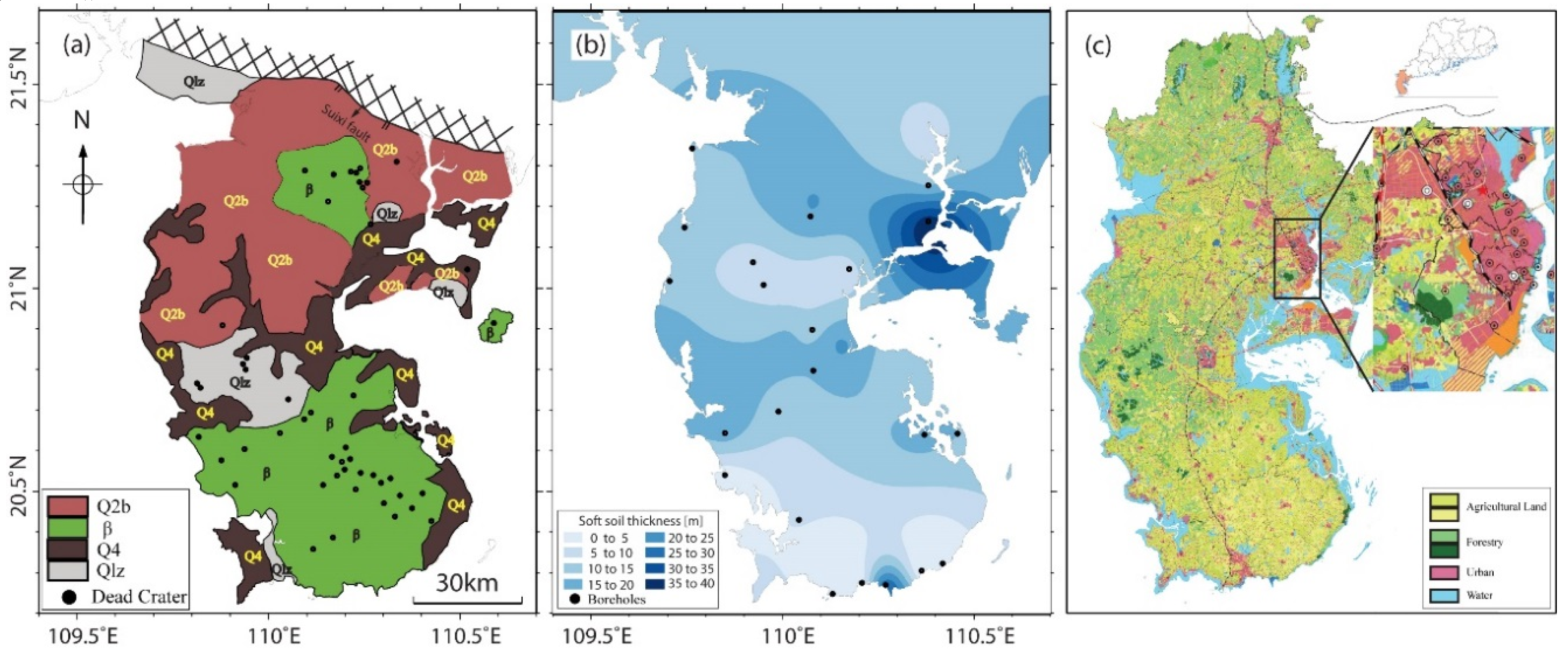
Figure 3.
Atmospheric delay and differential interferograms before and after pair wise logic calculation. (a) interferogram between image 20090209 and 20070204; (b) interferogram between image 20100212 and 20090209; (c) stacking interferogram after summing Figure 3a,b, aiming to reduce the atmosphere effects of image 20090209; (d) interferogram between image 20100212 and 2070204 after using direct interferometry; (e) the coherence histogram of Figure 3c,d. Black dashed lines in Figure 3a,b show areas with serious atmospheric delays and red rectangles in Figure 3c,d represent zones selected for coherence comparison. Red and blue solid lines in Figure 3e represent the coherence histogram of Figure 3c,d. (Date format: yyyymmdd).

Figure 4.
Exponential covariance function of velocity of each interferogram before (black) and after (red) atmosphere phase screen (APS) correction with our modified stacking method. (a–c) show results of the frame covering Zhanjiang city with JERS, ENVISAT, and ALOS1, respectively. Every black curve represents the statistical result of an interferogram in the stacking for each platform.
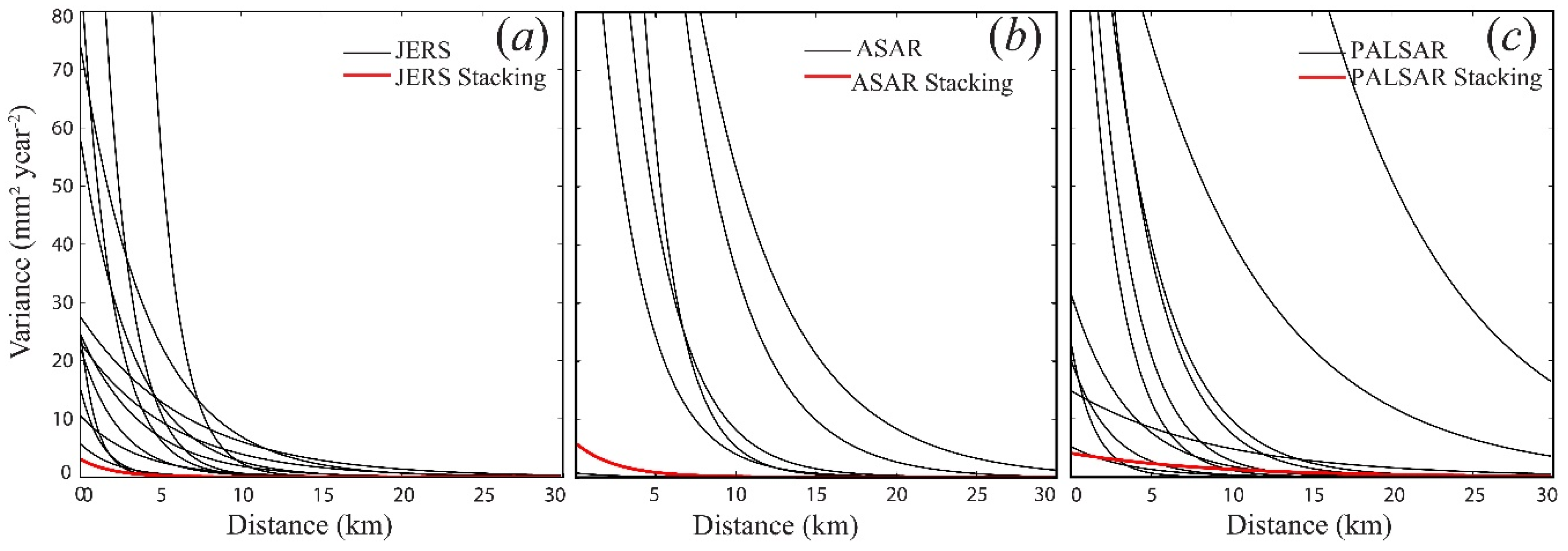
Figure 5.
Average subsidence velocity of the LZP from 1992 to 2010. (a) Mean velocity map of JERS from October 1992 to September 1998; (b) mean velocity map of ENVISAT from October 2003 to May 2007; (c) mean velocity map of ALOS1 from December 2006 to July 2010. Positive velocities (yellow) represent uplift, while the negative values (purple) indicate subsidence. Brown squares are representative of city’s locations. The red dashed rectangle is the representative subsidence area covering Zhanjiang city shown in Figure 7. Rectangle A, B, C, D, and E in Figure 5c are five representative areas in Figure 10. The locations are abbreviated as follows: the Leizhou Bay (L.Z.Bay), the Zhanjiang Bay (Z.J.Bay).
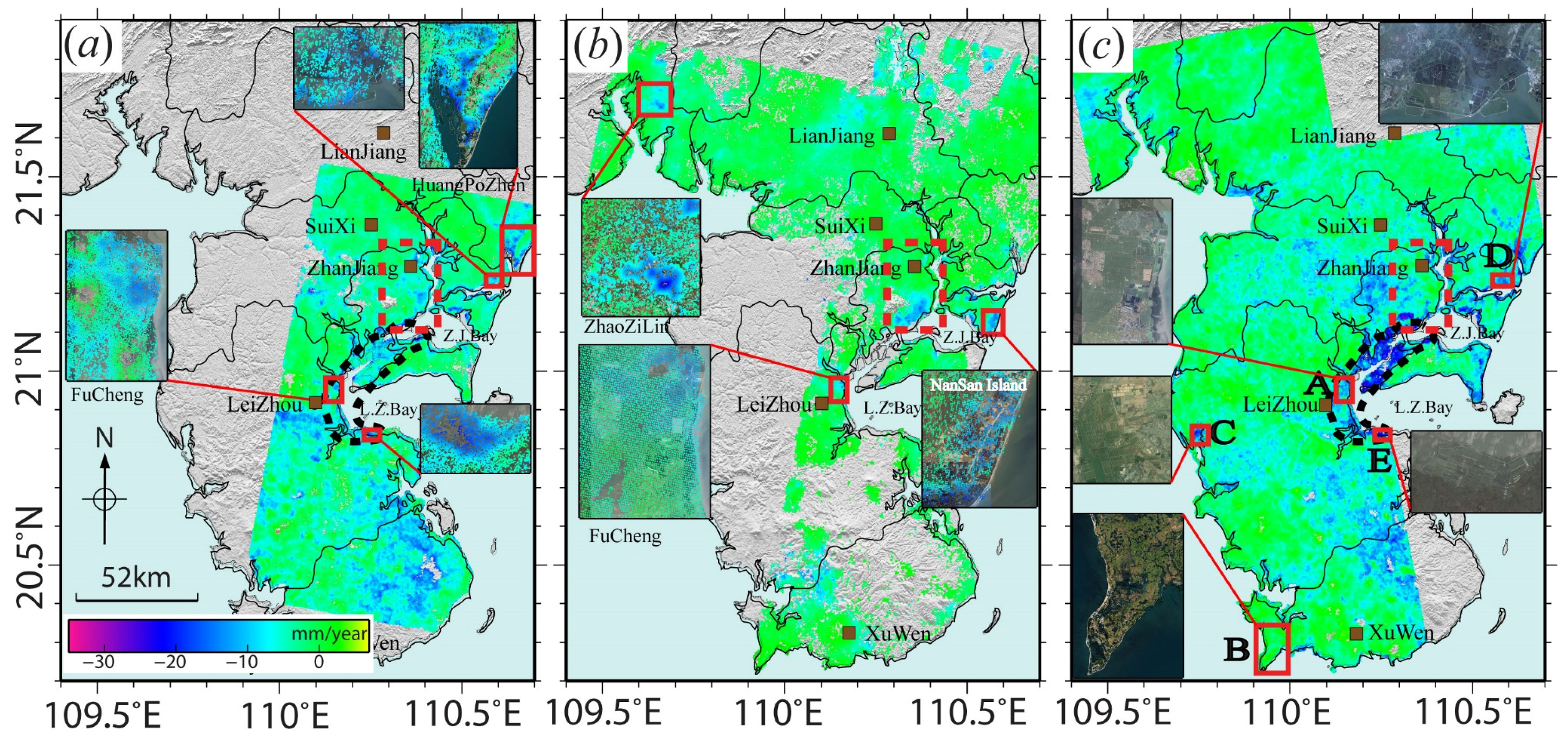
Figure 6.
Relationship between soft soil thickness and mean vertical velocity. The white bars represent the number of pixels and the red diamonds represent the calculated mean velocity for each soft soil thickness interval.
Figure 6.
Relationship between soft soil thickness and mean vertical velocity. The white bars represent the number of pixels and the red diamonds represent the calculated mean velocity for each soft soil thickness interval.

Figure 7.
The spatial-temporal evolution of land subsidence in Zhanjiang city. (a) Average subsidence rate of JERS from Octorber 1992 to September 1998; (b) average subsidence rate of ENVISAT from October 2003 to May 2007; (c) average subsidence rate of ALOS1 from December 2006 to July 2010. Zhanjiang city consists of four districts, namely Chikan, Xiashan, Potou, and Mazhang. Black dashed lines indicate the district border. Areas marked with red dashed lines are land subsidence bowls; Black circles are the leveling stations and two black solid lines are selected profiles of the subsidence bowl by aa’ and bb’.

Figure 8.
Deformation time-series of central points in four selected bowls, i.e., bowl 1, 4, 8, and 9, for each platform. The first row (a–d) represents the location of central points with optical backgrounds derived from GoogleEarth. The circles, diamonds, and triangles represent the location of JERS, ENVISAT, and ALOS1 respectively. Black words around the optical images are the adjacent land classes. The red star in (d) is a waterworks named Lindong started in 1999; The second to fourth rows represent the deformation time-series of four points for JERS, ENVISAT, and ALOS1. The red arrows represent the movement direction of land subsidence. The dashed lines in (e–p) are the results of linear fitting of the deformation time-series. The word ‘V=’ in (e–p) is the mean velocity in the vertical direction.
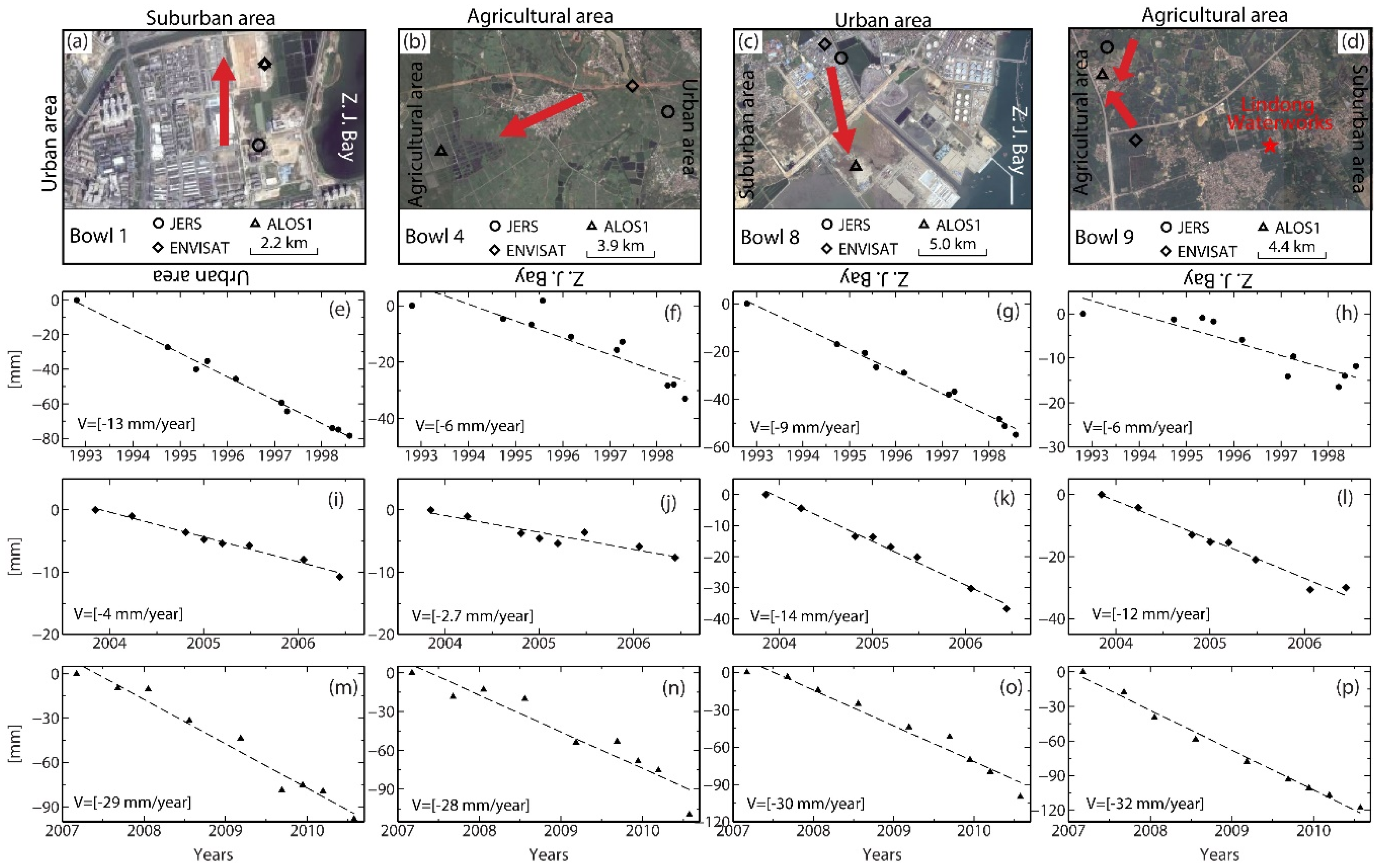
Figure 9.
Two bowl subsidence profiles (aa’ and bb’) in Figure 7. (a) aa’ profile going through subsidence bowl 6 and bowl 8 in the urban area. Two separated bowls, i.e., Bowl 6 and Bowl 8, represented by red merged into one bowl represented by green, and then became two connected bowls represented by blue; (b) bb’ profile going through subsidence bowl 9 in the suburban area, the mean velocity grows with increase of time. The red, green and blue solid lines represent the mean velocity of JERS, ENVISAT and ALOS1 datasets.
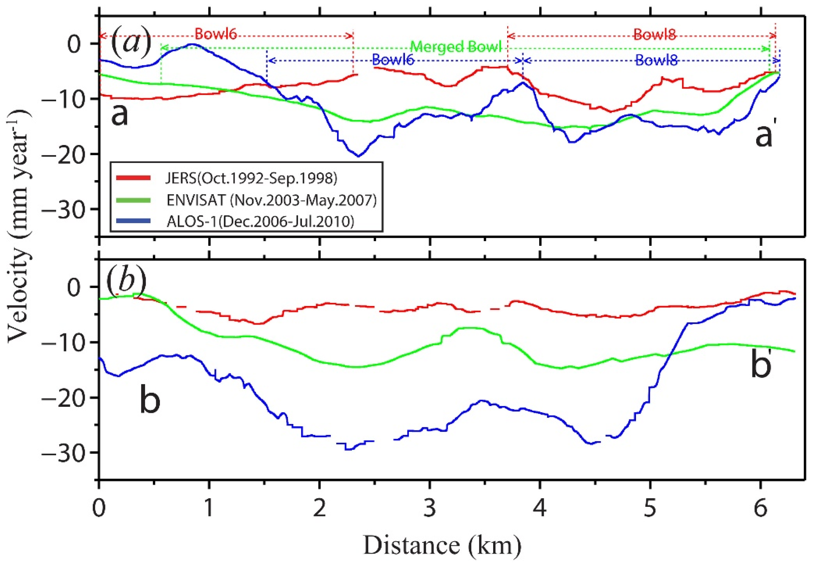
Figure 10.
Average deformation rate of the five representative coastal areas for ALOS1 dataset from December 2006 to July 2010. (a–e) are enlarged views of the red rectangles in Figure 4c. (a) is an area covered with large-scale farmlands, the maximum subsidence rate is 18 mm/year; (b) is located at the south of LZP with a maximum subsidence rate of 13 mm/year and a uplift rate of 3 mm/year; (c–e) are areas with large-scale aquaculture, the maximum subsidence rates are 23, 20, and 23 mm/year, respectively.

Figure 11.
Field photos of non-uniform subsidence of a building (a) and a pump facility (b), cracking and settlement of a channel (d) caused by over-exploiting groundwater in Fucheng town. (c) Flooded crops caused by rapid subsidence.
Figure 11.
Field photos of non-uniform subsidence of a building (a) and a pump facility (b), cracking and settlement of a channel (d) caused by over-exploiting groundwater in Fucheng town. (c) Flooded crops caused by rapid subsidence.

Table 1.
Area of subsidence bowls in Figure 7.
Table 1.
Area of subsidence bowls in Figure 7.
| Data | B1 (U) | B2 (U) | B3 (A) | B4 (A) | B5 (U) | B6 (U) | B7 (U) | B8 (U) | B9 (S) |
|---|---|---|---|---|---|---|---|---|---|
| Areas: km² (Bowl: B, Urban area: U, Agricultural area: A, Suburban area; S) | |||||||||
| JERS | 3.3 | 1.9 | 1.8 | 1.6 | 2.3 | 9.7 | 1.4 | 2.1 | 0.9 |
| ENVISAT | - | - | - | - | - | 10.7 | 2.8 | 10.8 | 4.3 |
| ALOS1 | 3.0 | 0.8 | 4.8 | 6.1 | 2.0 | 6.1 | 2.7 | 6.1 | 12.2 |
Table 2.
Comparison between Interferometric Synthetic Aperture Radar (InSAR) and leveling results.
| Comparison (mm/year) | JC18 | JC72 | JC53 | JC26 | JC55 |
|---|---|---|---|---|---|
| Leveling1989~1999 | −5 | −3.2 | −3.6 | −2.5 | −3.1 |
| InSAR_JERS1992~1998 | −7 | −5 | −6 | −4 | −5 |
| Difference | 2 | 1.8 | 2.4 | 1.5 | 1.9 |
Table 3.
Comparison of subsidence parameters in Mexico City [8,40,42], Jakarta of Indonesia [10,41], and the Leizhou Peninsula (LZP) [4].
| Urban areas | Mexico City (Chalco) | Jakarta of Indonesia | LZP |
|---|---|---|---|
| Aquifers | Lacustrine aquitard Granular aquifer Volcanic aquitard (0 < d < 300m) | Upper aquifer (<40 m) Middle aquifer (40 < d < 140 m) Lower aquifer (140 < d < 250 m) | Shallow aquifer (<30 m) Middle aquifer (30 < d < 200 m) Deep aquifer (200 < d < 500 m) |
| Sediments | Lacustrine deposits and Alluvial deposits of Quaternary | Quaternary sediments overlying Tertiary sediments | Unconsolidated alluvial and lacustrine overlaying the basement rocks of Neogene and Quaternary age. |
| Ava. extraction speed | 1990s: 7.8 m³/s | 1995: 1.5 m³/s | Until 2001: 6.7 m³/s |
| Max. velocity | <40 cm/year | <22 cm/year | <3.2 cm/year |
| Water level decline speed | 1.5 m/year | 0.1–1.9 m/year | 0.1–0.8 m/year |
| Correlation with surface geology | Thickness of deposits | Land use | Thickness of soft soil/Land use |
| Agricultural areas | Mexico City(Chalco) | Jakarta of Indonesia | LZP |
| Max. velocity | <18.4 cm/year | 15.1 cm/year | <2.5 cm/year |
| Surface geology | Compressible deposits | Surficial deposits | Volcanic basalt |
| Correlation with geology | Type of compressible deposits | Correlate with land use | Thickness of soft soil |
© 2017 by the authors. Licensee MDPI, Basel, Switzerland. This article is an open access article distributed under the terms and conditions of the Creative Commons Attribution (CC BY) license (http://creativecommons.org/licenses/by/4.0/).
Share and Cite
MDPI and ACS Style
Du, Y.; Feng, G.; Peng, X.; Li, Z. Subsidence Evolution of the Leizhou Peninsula, China, Based on InSAR Observation from 1992 to 2010. Appl. Sci. 2017, 7, 466. https://doi.org/10.3390/app7050466
AMA Style
Du Y, Feng G, Peng X, Li Z. Subsidence Evolution of the Leizhou Peninsula, China, Based on InSAR Observation from 1992 to 2010. Applied Sciences. 2017; 7(5):466. https://doi.org/10.3390/app7050466
Chicago/Turabian StyleDu, Yanan, Guangcai Feng, Xing Peng, and Zhiwei Li. 2017. "Subsidence Evolution of the Leizhou Peninsula, China, Based on InSAR Observation from 1992 to 2010" Applied Sciences 7, no. 5: 466. https://doi.org/10.3390/app7050466
Note that from the first issue of 2016, this journal uses article numbers instead of page numbers. See further details here.