Article

A Study of the Transient Response of Duct Junctions: Measurements and Gas-Dynamic Modeling with a Staggered Mesh Finite Volume Approach

by
Antonio J. Torregrosa
*,
Alberto Broatch
,
Luis M. García-Cuevas
and
Manuel Hernández
CMT–Motores Térmicos, Universitat Politècnica de València, 46022 Valencia, Spain
*
Author to whom correspondence should be addressed.
Appl. Sci. 2017, 7(5), 480; https://doi.org/10.3390/app7050480
Submission received: 20 March 2017 / Revised: 28 April 2017 / Accepted: 2 May 2017 / Published: 8 May 2017
(This article belongs to the Special Issue Internal Combustion Engines (ICE) for Ground Transport)

Abstract

:
Duct junctions play a major role in the operation and design of most piping systems. The objective of this paper is to establish the potential of a staggered mesh finite volume model as a way to improve the description of the effect of simple duct junctions on an otherwise one-dimensional flow system, such as the intake or exhaust of an internal combustion engine. Specific experiments have been performed in which different junctions have been characterized as a multi-port, and that have provided precise and reliable results on the propagation of pressure pulses across junctions. The results obtained have been compared to simulations performed with a staggered mesh finite volume method with different flux limiters and different meshes and, as a reference, have also been compared with the results of a more conventional pressure loss-based model. The results indicate that the staggered mesh finite volume model provides a closer description of wave dynamics, even if further work is needed to establish the optimal calculation settings.

1. Introduction

Duct junctions are essential elements of numerous piping systems, including the intake and exhaust systems of reciprocating internal combustion engines. The use of one-dimensional time domain gas-dynamic codes has become commonplace in the numerical study of unsteady flows in such systems, both in terms of their effect on engine performance and on intake and exhaust orifice noise [1]. While assuming one-dimensional wave action may be acceptable when duct diameters are relatively small, as is the case in the majority of the ducts present in engine intake and exhaust systems of passenger car engines, in certain elements, and most notably in duct junctions, complex three-dimensional flow structures may occur [2]. Consideration of the effects of such structures on the one-dimensional flow in the adjacent ducts requires the definition of suitable boundary conditions at the junction, usually involving empirical information.
The effects of a junction on the flow in the neighboring ducts arise in different ways. From the point of view of the passive propagation of small amplitude pressure waves (i.e., in the acoustic range) the effect can be characterized in terms of length corrections, which have been reported to depend on the type of side-branch and the branch width and length [3], and with a rapid increase in the duct length corrections being associated with the excitation of non-planar higher order modes, which also results in lower sound transmission. This sort of representation has been quite successfully applied to the prediction of the effect on intake noise of a multi-pipe junction in the intake manifold [4]. It has also been reported [5] that for low Strouhal numbers based on the duct diameter, the acoustic transmission properties of T-junctions can be acceptably described by using an incompressible quasi-steady model, the upper limit of the Strouhal number being defined by flow-acoustic interaction effects, which differ significantly between different flow configurations: waves incident on the junction at the downstream side are attenuated, whereas waves incident at the other branches may be either amplified or attenuated, depending on the Strouhal number [6]. Such flow-acoustic interactions due to the coupling of the flow and the geometry are common to all intake and exhaust system elements [7].
When the focus is on the effect of the junction on the propagation of finite amplitude pressure waves and the resulting influence on engine performance, different approaches are found in the literature, most of them inspired by the seminal work of Benson [8]. The simplest approach is given by constant pressure models, in which is it assumed that the pressure at the end of all branches of the junction is the same at any time, so that the pressure is assumed to be uniform across the junction. The most comprehensive description of these models is given in [9], where it was shown that, besides the assumption of uniform pressure, additional closing equations must be added. While the choice of those equations is arbitrary, it was also shown in [9] that assuming that the total enthalpy for all the outgoing flows is the same provides suitable results.
More elaborated approaches are based on the consideration of the pressure differences existing between the different branches, which are incorporated in a quasi-steady manner, i.e., steady pressure loss coefficients (or more properly, as discussed in detail in [10], energy change coefficients accounting partly for losses and partly to a mutual energy transfer between the partial flows) are applied at each time step. The solutions proposed differ mainly in the origin of the pressure loss coefficients, in the hypotheses underlying their determination, and in the precise implementation of the solution method.
Regarding the origin of the coefficients, while there have been some attempts to obtain them from computational fluid dynamics (CFD) simulations [11,12,13], it appears that the results are strongly dependent on the numerical method used, both in the details of the flow and in the overall values of the coefficients obtained [14]. Therefore, usually the coefficients are either obtained from simple and robust models, or specific measurements are performed in order to characterize the junction under consideration. The most successful example of the first option is probably that presented in [15], where a remarkable agreement with experimental results was obtained from a model that extended the previous work performed in [16] and neglected any effects of mixing losses, compressibility and wall friction. Regarding the experimental characterization, it is usual to consider steady incompressible flow, as in [17], but more recently, specific studies accounting for the flow compressibility have been reported [18,19] that suggest that the total pressure loss coefficient is mainly dependent on the Mach number, mass flow rate ratio, and area ratio, and is almost independent of the Reynolds number.
Numerous implementations of the pressure loss model for multi-pipe junctions have been proposed in the literature, comprising implicit time formulations [20] and different explicit solutions, such as the supplier–collector strategy [21], the branch superposition method [22] and the generalization of the classical approach of Benson presented in [23]. The limitations of these approaches lie mainly in the fact that, even if steady flow coefficients contain information on three-dimensional separation effects around the junction, the results will be significant only if quasi-steady flow can be assumed, which requires that mass and energy storage at the junction are very small, which may not be the case in real manifold flows. Additionally, any information regarding the wave refraction characteristics of the junction is lost in the quasi-steady approximation.
Overcoming these limitations requires accounting for the unsteady and multi-dimensional character of the flow at the junction, but without incurring in an excessive computational cost. A suitable solution is thus to include a local multi-dimensional region within an otherwise one-dimensional wave-action engine simulation, as first suggested in [24]. In this first approach, an inviscid two-dimensional model was applied to the simulation of shock-wave propagation through different junctions, and the observed evolution of the wave fronts through the junctions and the measured high frequency pressure oscillations induced by the transverse reflections were successfully predicted. However, even if the increase in the computational cost was reasonable, it did not appear to be justified when compared with a conventional quasi-steady pressure loss model [25].
It appears, thus, that a full three-dimensional description of the junction should be used in order to describe its unsteady behavior. Such a description was presented in [26,27], successfully reproducing the flow field and the associated non-plane-wave motion. However, even if coarse 3D grids were used in the first simulation cycles that were switched to more refined grids during the last simulation cycles, the computational cost and time may still be regarded as excessive for the practical design and evaluation of full intake and exhaust systems.
A possible alternative to 1D–3D coupling, which could provide some accountancy for the three-dimensional effects at the junction and to the authors’ knowledge has not been explored in some detail, would be the use in this context of a staggered mesh finite volume method [28]. Such methods have become standard in commercial codes, either as the core solver [29,30], or used locally for elements exhibiting significant three-dimensional features, such as plenums and mufflers [31]. Typically, when these methods are applied to simple duct junctions, a single volume is used for the junction with appropriate effective areas and characteristic lengths at each connection with the adjacent ducts. As these connections contain information on vector quantities (including the orientation of the branch duct) the momentum equation can be solved, even in an approximate way, so that all the effects of the junction of the flow need not be included through the pressure loss coefficients. Additionally, it would be possible to use a refined mesh locally at the junction, so that a first-order estimate of any three-dimensional features could be obtained.
The objective of this paper is precisely to establish the potential of these ideas as a way to improve the description of the effect of simple duct junctions on an otherwise one-dimensional flow system, as the intake or exhaust of an internal combustion engine. Specific experiments have been performed in order to obtain precise and reliable results on the propagation of pressure pulses across junctions. The results obtained have been compared to simulations performed with different versions of a staggered mesh finite volume method and different meshes and, as a reference, also with the results of a more conventional pressure loss-based model.

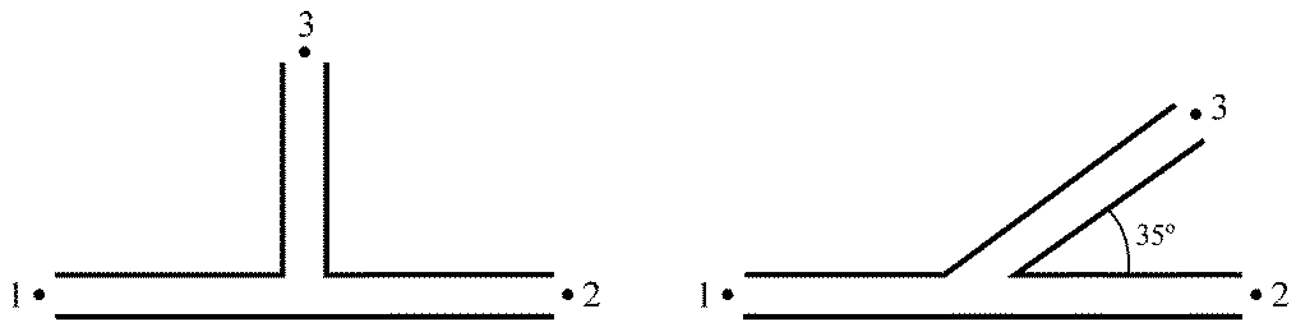
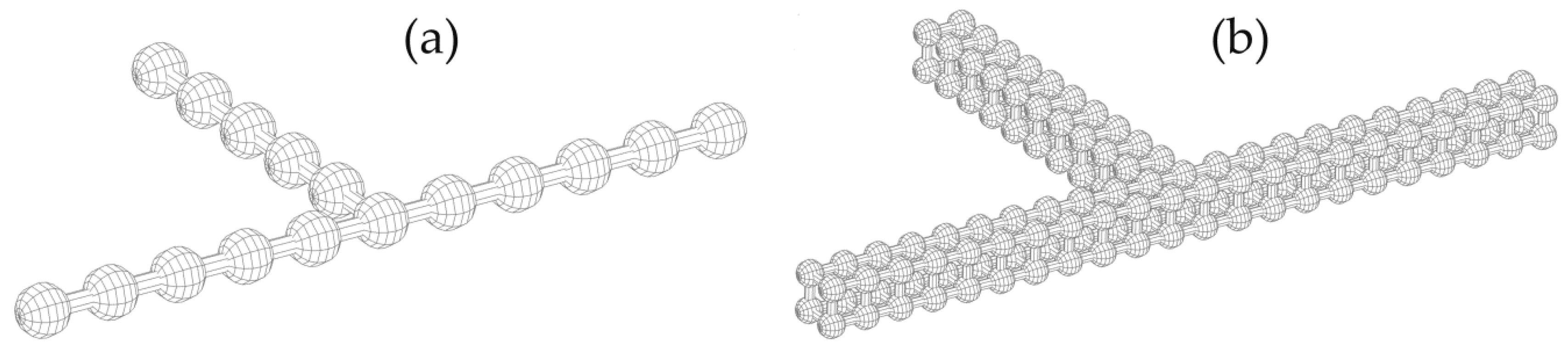
2. Materials and Methods

Two junctions, shown schematically in Figure 1, were manufactured. A T-junction and a Y-junction were considered, in order to allow the analysis of the effect of the angle of the side branch. An internal diameter of 51 mm was used in all the branches of the junctions.
While several formalisms may be used for the representation of the transient response of a system, the most intuitive one for the present case of a junction is that based on the consideration of wave components, so that the junction is actually regarded as a multi-port. In this framework, for a junction such as that represented in Figure 2, one has three excitations and three responses, and writing the relations between them directly in matrix form in the frequency domain, one has:
[ B 1 B 2 B 3 ] = [ R 1 T 21 T 31 T 12 R 2 T 32 T 13 T 23 R 3 ] [ A 1 A 2 A 3 ] .
where, as indicated in Figure 2, A i represents the wave component moving towards the junction in port i and B j represents the wave component moving away from the junction in port j . Regarding the matrix elements,   R i denotes the reflection coefficient as seen from port i whereas T i j denotes the transmission coefficient between ports i and j . All these magnitudes are functions of the frequency f .
In this way, one has a reflection coefficient for each of the pipes arriving at the junction, and transmission coefficients for all the possible transmission paths, indicated by the corresponding subscripts. The experimental setup and the corresponding measurement procedure are described in detail in [32,33], and here only a brief overview is given in Appendix A.
Two different modeling approaches were evaluated: a staggered mesh finite volume method and, as a reference, a more conventional pressure loss-based model. The staggered mesh finite volume method used is described in detail in [34], where a flux-corrected transport (FCT) technique was used in order to suppress the spurious oscillations that these numerical methods exhibit in the vicinity of discontinuities in the flow variables. It was found that satisfactory results were obtained through the combination of dissipation via damping together with the phoenical form of the anti-diffusion term. As an alternative, the momentum diffusion term described in [35] was also used. A brief summary is given in Appendix B.
The pressure loss-based model uses a conventional one-dimensional finite volume model with a collocated mesh, derived from the code available in [36]. The junction is modeled as a small volume with three connections to which different pressure loss coefficients are assigned, and in which the mass and energy conservation equations are solved. For the connection to the duct where the incident pressure pulse propagates it has been assumed that the total pressure loss is zero, whereas for the other two connections their corresponding pressure loss coefficients are computed following the expressions given in [15,16]. The procedure is summarized in Appendix C.

3. Results and Discussion

In this section, first the experimental results obtained will be analyzed, both in the time ( t ) and the frequency ( f ) domains. Then, the performance of the different modeling approaches will be discussed, first in the case in which the junction itself is represented by a zero-dimensional element, and secondly in the case in which the staggered mesh method is used to provide a quasi-3D description of the junction.

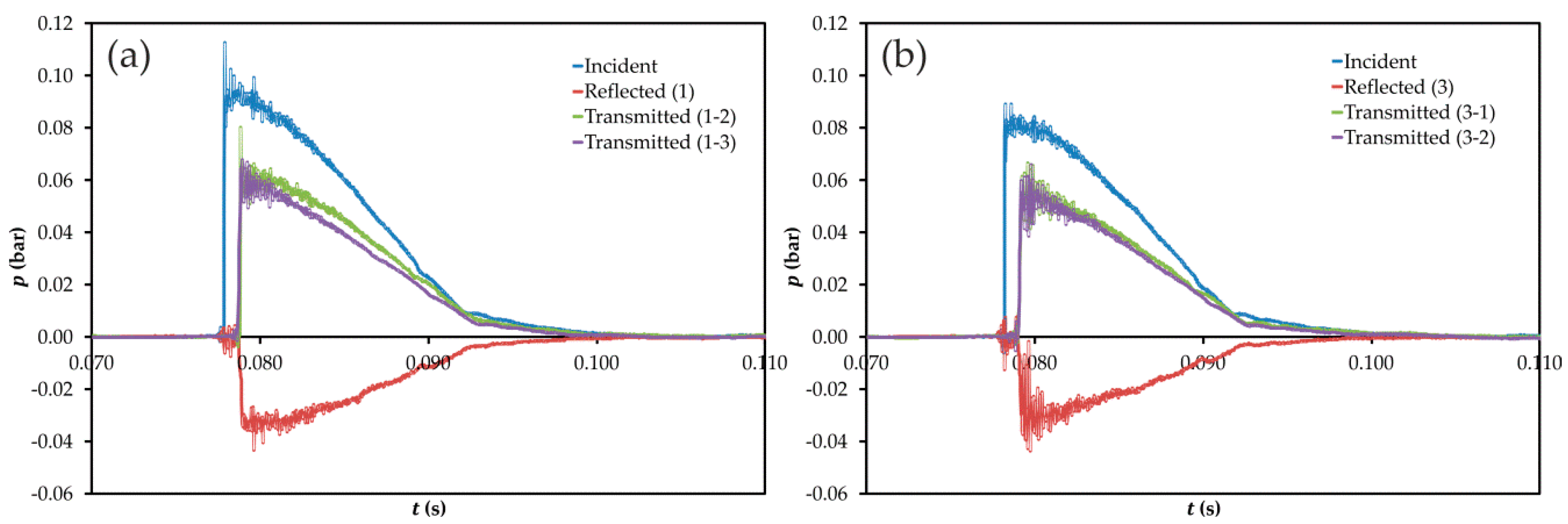
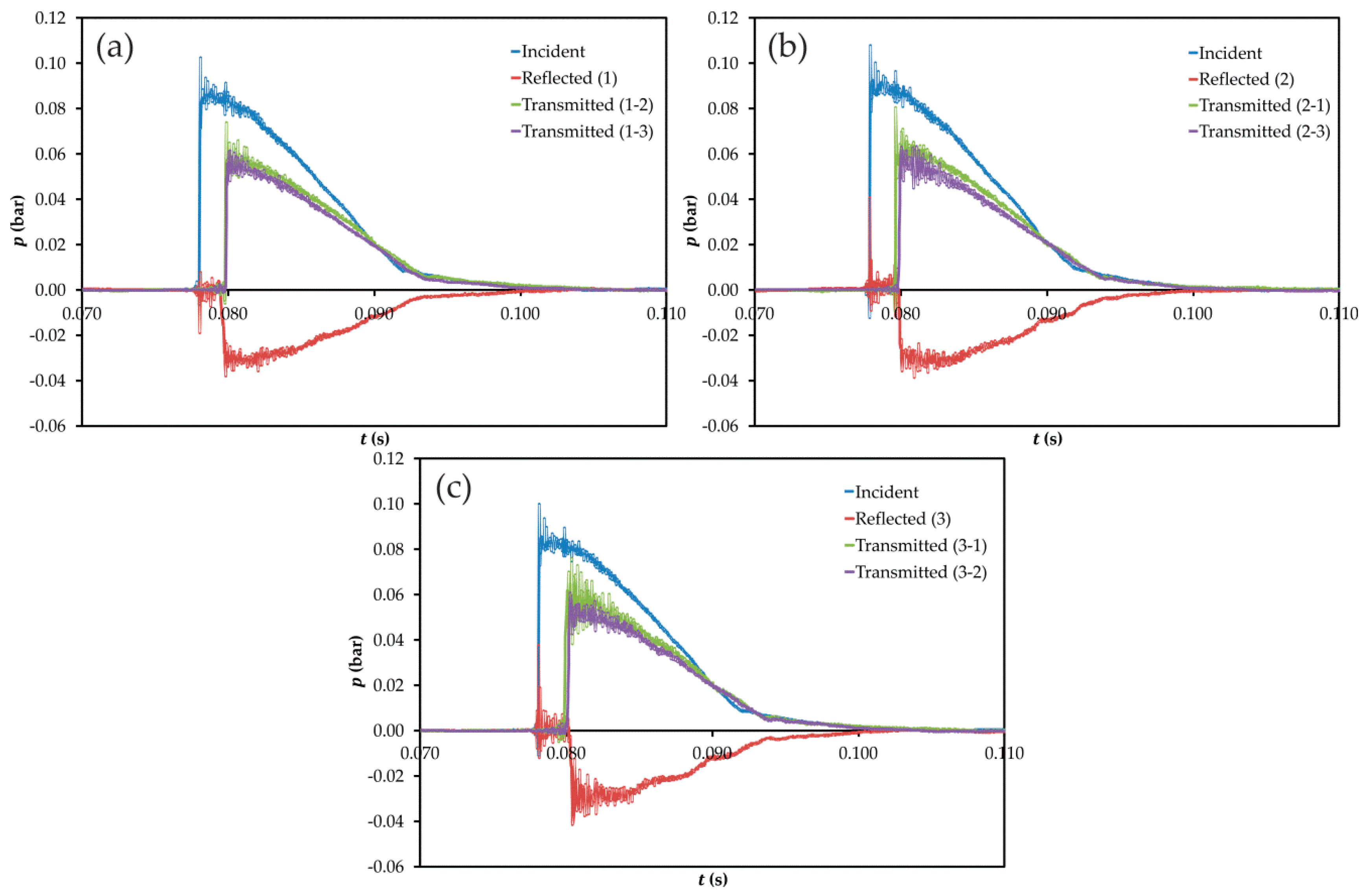
3.1. Experimental Results

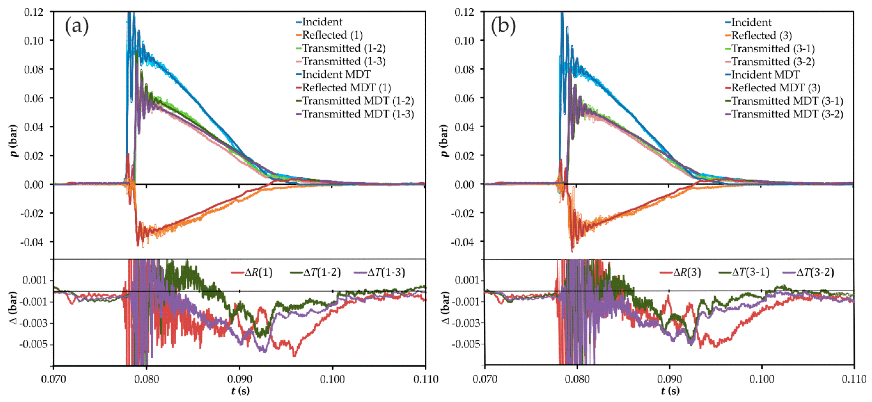
3.1.1. Time Domain Analysis

The results for the T-junction and shown in Figure 3. Ports are denoted as in Figure 1, and it is apparent that when the junction is excited at port 1 the pulse transmitted through port 2 (i.e., in the main propagation direction) has a higher amplitude than that transmitted through port 3 (the branched duct), as could be intuitively expected. It is also apparent, and equally expectable, that when the junction is excited at port 3, the pulses transmitted through ports 1 and 2 are very similar, the small differences observed being attributable to manufacturing issues.
Differences in the reflected pulses recorded at ports 1 and 3 are also apparent, even if the incident pulses do not have the same amplitude. The reflected pulse recorded at port 3 is noisier, and its amplitude is comparable to that of the reflected pulse recorded at port 1, while the corresponding incident pulse has a lower amplitude. This indicates that reflection is more intense when the junction is excited at the branch duct, as it is also intuitively reasonable in terms of the interaction of the incident pulse with the wall of the main duct. Of course, none of these effects, regarding both transmission and reflection, can be accounted for by a constant pressure model, and this is the reason why such a model will not be considered in the subsequent discussion.
The results for the Y-junction are shown in Figure 4. Here the trends observed confirm those found for the T-junction regarding the difference between the main duct and the branch duct, but with additional issues related with the branch angle. Comparison of Figure 4a,b indicates that the difference in amplitude between the two pulses transmitted is more important when the branch direction is against that of the incident pulse (i.e., when the junction is excited at port 2), in which case the results are rather similar to those shown in Figure 3a for the T-junction. Regarding the reflected pulses recorded at ports 1 and 2, some differences may be observed mostly in the last part of the pulse, which suggests some difference in the dynamic behavior of the junction.
These statements are supported by the results obtained with the excitation at port 3, shown in Figure 4c. Here, it appears that again the amplitude of the transmitted pulse is higher when there is no significant change in direction along the transmission path (in this case, from port 3 to port 1). However, the differences are not as apparent as those seen in Figure 4b, which is reasonable considering that here there is some change in direction in the two transmission paths. It is also worth noticing the clear differences observed between the reflected pulse recorded at port 3 and those recorded at the other two ports. A much more complex time evolution can be observed in the case of port 3, which again suggests that wave dynamics inside the junction depend significantly on the port at which the junction is excited.

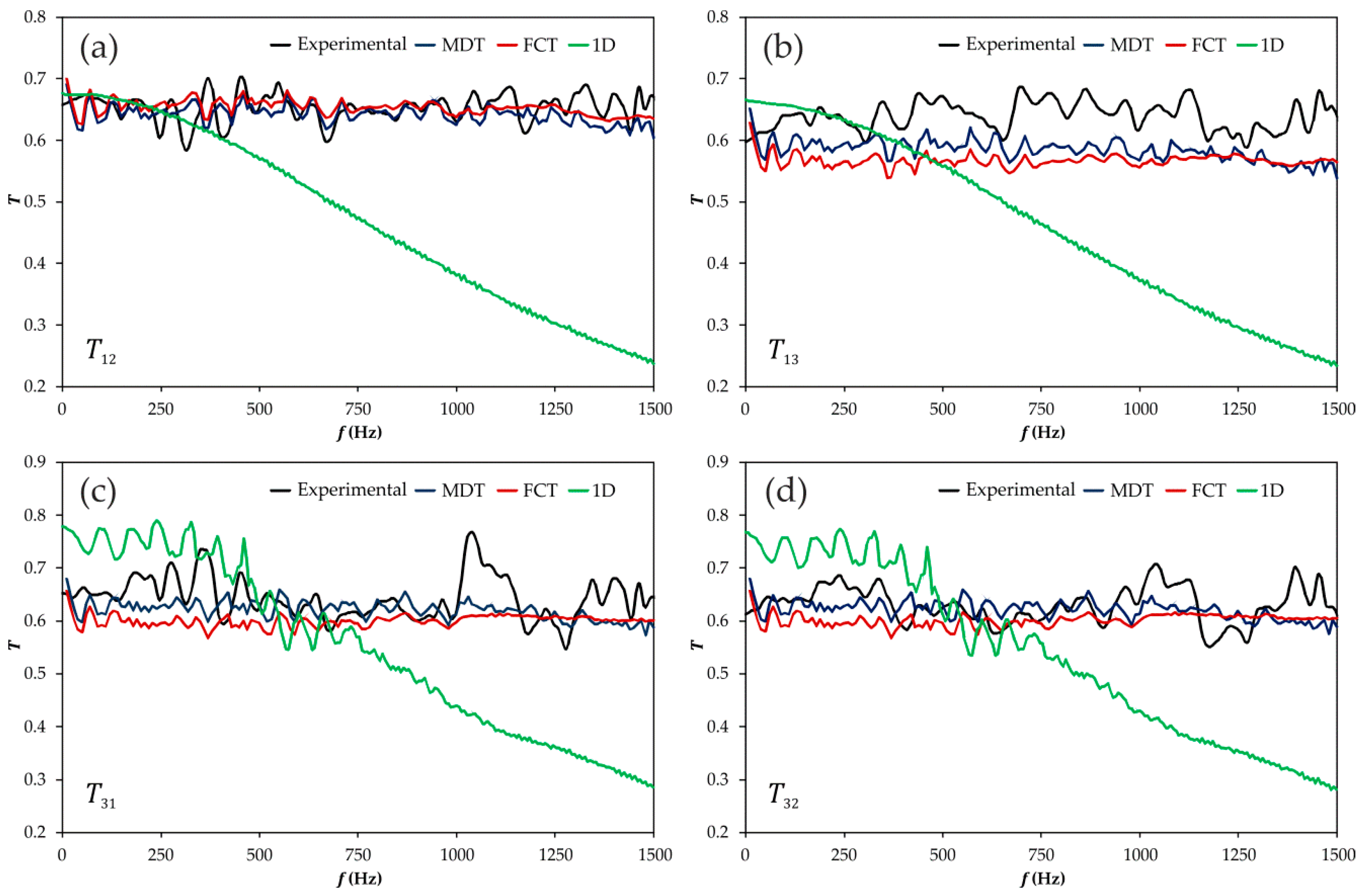
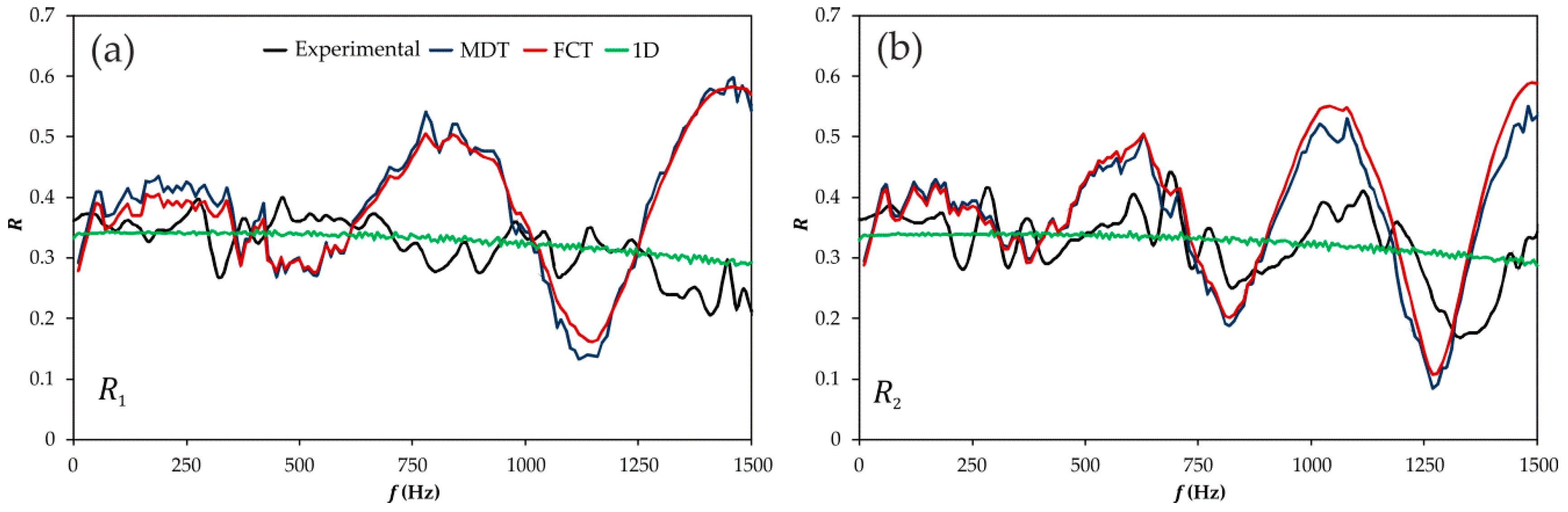
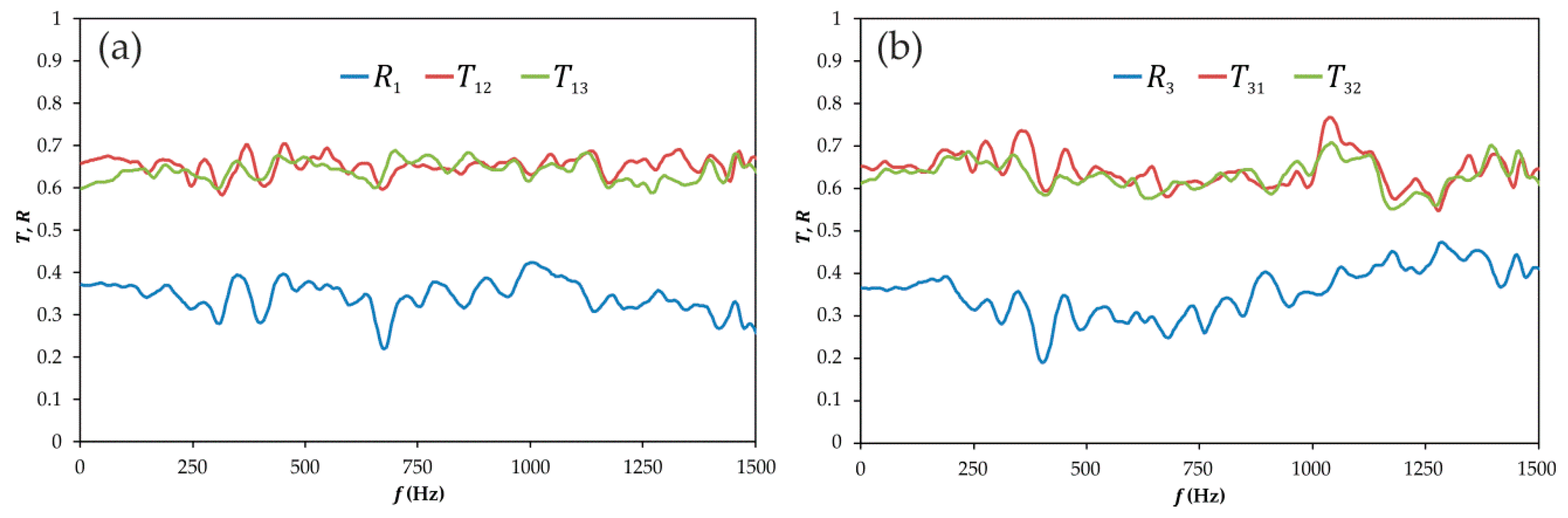
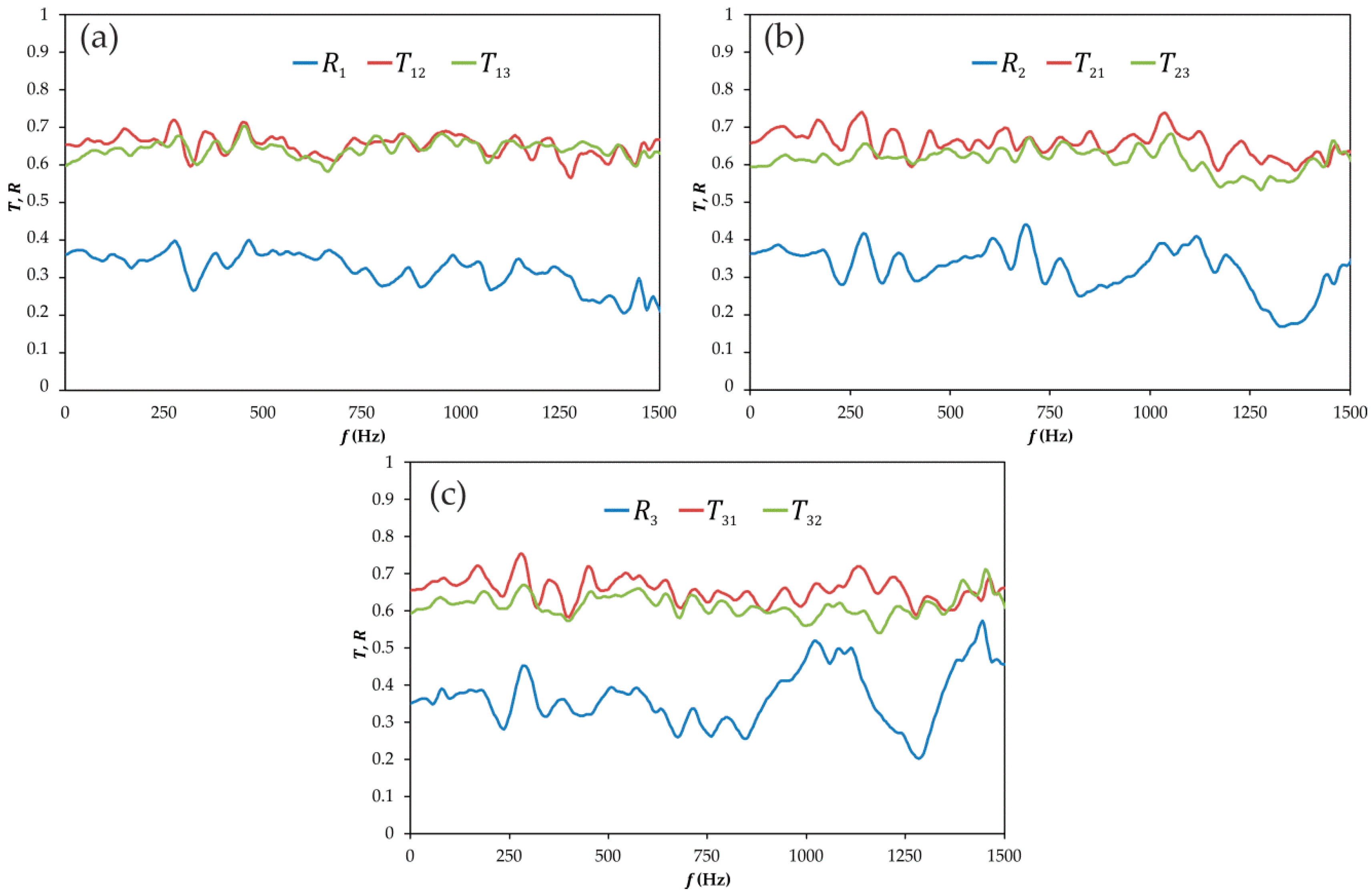
3.1.2. Frequency Domain Analysis

Here, the results obtained for the transmission and reflection coefficients defined in Equation (1) are analyzed. For brevity, only the modulus of these coefficients will be considered, as this contains significant information about the overall energetic behavior of the junction. The results for the T-junction are shown in Figure 5, where it can be observed that the values obtained in the very low frequency range (below 200 Hz) are fully consistent with the time domain results shown above in Figure 3: when exciting the junction at port 1, it is seen that | T 12 | is systematically larger than | T 13 | in this frequency range, whereas when the excitation is at port 3 the differences between | T 31 | and | T 32 | are significantly smaller.
At higher frequencies, above 200 Hz, it can be seen that the behavior of | T 12 | and | T 13 | is essentially flat around mean values of 0.65 and 0.64, respectively, with a maximum deviation from the mean of 0.065 in | T 12 | and of 0.05 in | T 13 | . On the contrary, in the case of | T 31 | and | T 32 | their mean values are very similar to those of | T 12 | and | T 13 | (0.64 and 0.63, respectively) but some relevant acoustic features can be detected in both coefficients between 1000 and 1250 Hz, mostly in the case of | T 31 | where the deviation from the mean value reaches a maximum of 0.125, while | T 32 | follows the same trend but with a maximum deviation from the mean of 0.08 . This confirms, on one hand, that when the junction is excited at port 3 the two propagation paths are substantially equivalent and, on the other hand, that their behavior is different from that obtained when exciting the junction at port 1.
This second statement is fully supported by the spectra of the reflection coefficients | R 1 | and | R 3 | : it is apparent that | R 3 | is overall larger than | R 1 | for frequencies below 200 Hz, as suggested by the results shown in Figure 4, but now without any uncertainty due to the difference in amplitude between the incident pulses used in each test. Additionally, the trend observed is rather different for frequencies above 200 Hz, and most notably above 1000 Hz, where | R 1 | shows a certain decreasing tendency whereas | R 2 | increases with frequency.
The corresponding results for the Y-junction are shown in Figure 6. Again, results below 200 Hz confirm the time domain tendencies observed in Figure 4. In this frequency range, it is seen that while | T 12 | is only slightly higher than | T 13 | , when exciting at ports 2 or 3 one finds that the transmission coefficient corresponding to a smaller change in direction (that is, | T 21 | when exciting at port 1 and | T 31 | when exciting at port 3) is significantly larger than the other one, and that this effect is more noticeable the larger is the change in direction.
When considering frequencies above 200 Hz, noticeable differences are also observed between the case with excitation at port 1, for which results very similar to those shown in Figure 5a are obtained, with small differences between | T 12 | and | T 13 | and an almost flat behavior with little dependency on frequency, and the other two cases, in which the transmission coefficients corresponding to the propagation path with the smallest change in direction ( | T 21 | and | T 31 | ) are significantly and systematically higher than those implying an important change ( | T 23 | and | T 32 | , respectively) except at the highest frequencies represented.
However, it is in the reflection coefficients where the effect of the change in the excitation port is more apparent. In fact, the results for | R 1 | do not differ substantially from those obtained for the T-junction and shown in Figure 5a, neither in the low frequency values nor in the high frequency trend. On the contrary, the high frequency behavior seen in | R 2 | and | R 3 | is a clear indication of the change produced in the dynamic characteristics of the junction when the excitation port is changed, an effect that could be guessed from the time domain results of Figure 4 but now is fully confirmed. Actually, a well-defined trend of picks and troughs can be observed in both cases, with similar shape but a clear frequency shift, which provides a sort of acoustic signature of the dynamic behavior of the junction. The fact that such a behavior is not apparent in the spectrum of | R 3 | for the T-junction shown in Figure 5b indicates that such dynamic issues are suppressed by the symmetric nature of the excitation through a perpendicular branch.

3.2. Assessment of Modelling Approaches Considering a 0D Description of the Junction

Here, modeling approaches in which the junction itself is regarded as a 0-dimensional element, while the flow in the adjacent ducts is assumed to be one-dimensional, will be evaluated. In the context of the staggered mesh finite volume method, this corresponds to the case in which the junction is regarded as a single volume and the adjacent ducts are meshed only in the axial direction. The pressure loss-based model used here falls also within this category since, as commented in Appendix C, the junction branches are connected through an auxiliary 0D element.
Again, separate analyses for the time and the frequency domains are presented.

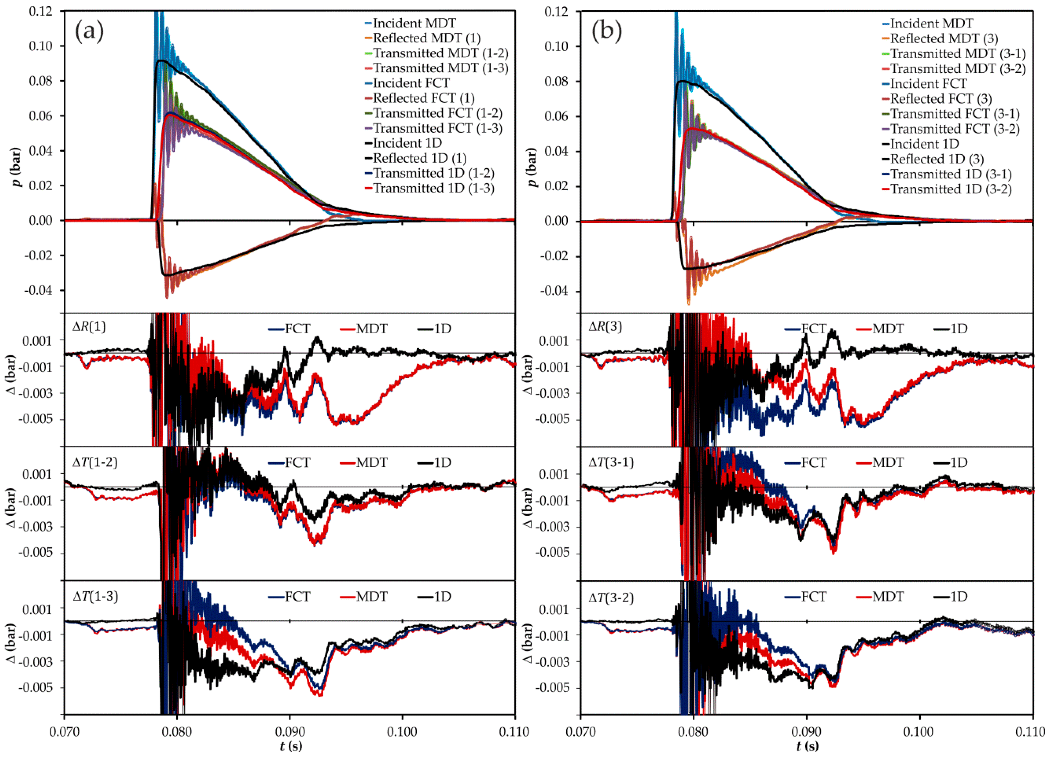
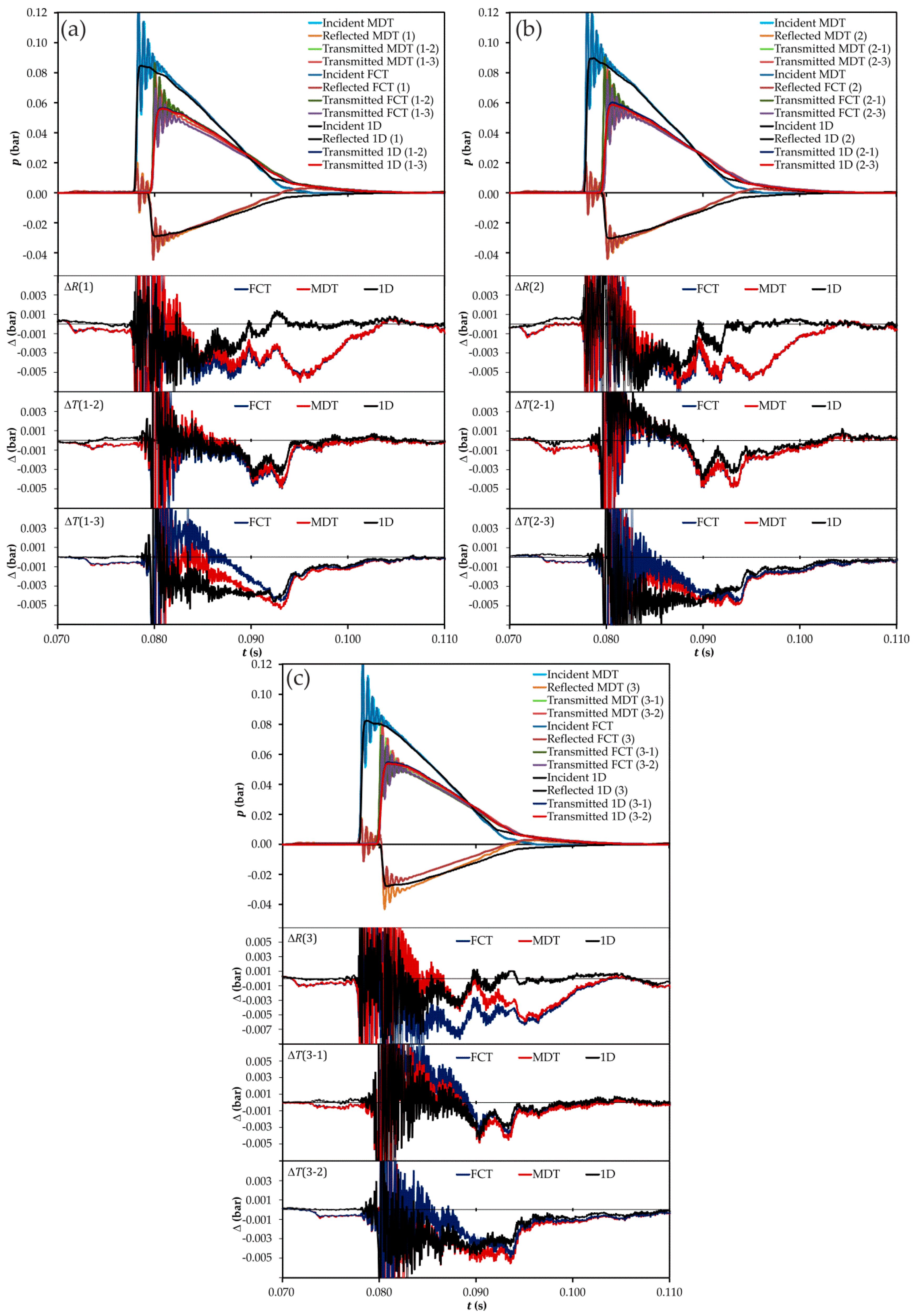
3.2.1. Time Domain Assessment

First, in Figure 7, direct comparison between the experiments and the method with the momentum diffusion term (MDT) as flux limiter is given for the case of the T-junction. The figures at the top provide a direct representation of the results obtained, whereas in the figures at the bottom the differences between the experimental and numerical results are represented (these are labeled Δ R and Δ T for reflected and transmitted pulses, respectively). In general, the model reproduces the experimental results within reasonable limits, but with a superimposed oscillation due to the development of the pulse from station 0 to station 1 (refer to Figure A1) and which is a consequence of the way in which the inlet boundary condition has been set. The scale of the vertical axis in the differences plots has thus been chosen so as to allow proper comparison for the times not affected by those oscillations.
From the differences plots, it is apparent that the numerical results tend to underestimate the actual measured values in the trailing part of the pulses, for t > 0.85 s, the differences being larger in general for the case of the reflected pulse. The situation is rather more complex for the previous instants, with different trends observed for the transmitted and reflected pulses, and with a noticeable influence of the port at which the junction is excited.
The results obtained for the rest of the modeling approaches considered are compared in Figure 8, where for clarity the experimental results are not shown in the top figures, but the bottom figures have been expanded to allow proper analysis of the behavior observed in each of the propagation paths. It is apparent that the conventional pressure loss method (labeled 1D in the figure) is much less dispersive than any of the staggered-grid methods, and thus better suited for this particular calculation setting. This is particularly true in the case of the reflected pulses, where the conventional method approaches the measured values considerably earlier. It is also apparent that while no significant differences can be found between the MDT and the FCT methods in the reflection seen from port 1, this is not the case when the junction is excited at port 3: the FCT method exhibits larger differences, except in the last part of the reflected pulse.
Regarding the different transmission paths, it can be observed that, while relatively small differences between all the methods are seen in the case of transmission from port 1 to port 2 (the performance of the conventional method being slightly better), significant differences appear at intermediate times in all the cases in which port 3 is involved. There is a clear trend in the results obtained in these cases, in the sense that the conventional method produces the lowest values, the FCT method the highest values, and those produced by the MDT method lie in between. However, the maximum differences are observed at time instants in which the amplitude of the transmitted pulses is relatively high.
As an additional criterion for the comparison of the performance of the different modeling approaches, the mean quadratic error corresponding to the differences shown in Figure 8 was computed. A time window with 0.82 < t < 0.95 was chosen to avoid the large oscillations and to focus on those times for which the differences between the methods are more apparent.
The values obtained for the mean quadratic errors are summarized in Table 1, where it is confirmed that the best values for the reflection coefficients are those provided by the conventional method, while the FCT method gives the best approach to the transmission coefficients.
Similar comments can be made about the comparison shown in Figure 9 for the case of the Y-junction. Again, the conventional method reproduces better the behavior of the reflected pulses, regardless of the excitation port, and the MDT and the FCT methods exhibit significant differences only when the junction is excited at port 3, following the same trend as for the T-junction.
The trend is also very similar for the different transmission paths. Transmission between ports 1 and 2 is acceptably reproduced by all the modeling approaches, regardless of the exciting port, again with a slightly better performance of the conventional model. In those cases in which port 3 is included in the transmission path, the tendency observed is again the same when the junction is excited at port 1 or 2, with a small difference with respect to the T-junction when the excitation comes from port 3: in this case, the lowest values are those provided by the MDT method, most notably in the transmission from port 3 to port 2.
Again, the mean quadratic errors were calculated, and the corresponding results shown in Table 2 confirm the previous comments.
From these results, it is apparent that the conventional pressure loss model, while is not able to account for all the differences observed between the two transmission paths studied in each test, could still provide a sufficient approximation to the real situation if the focus of the problem is on the reflection properties of the junction and only time domain issues are relevant for the problem under study (for instance, the eventual influence of a reflection at an intake junction on the volumetric efficiency on the engine). The staggered mesh finite volume method appears to be more sensitive to the relative directions of the different branches, mostly when the excitation comes from the side branch (port 3), as should be expected since the momentum equation is actually solved, albeit in an approximate way, at the junction, whereas in the conventional model such effects are included only through their influence on the pressure loss coefficients.

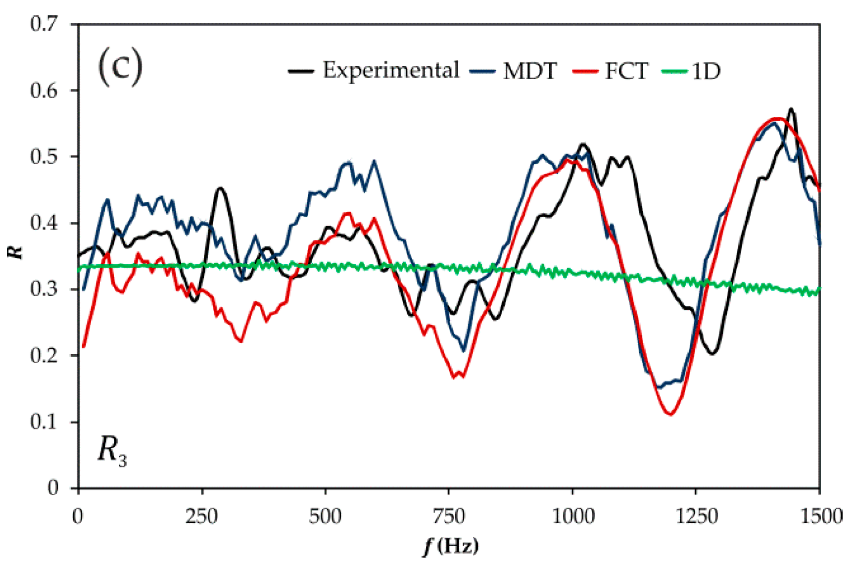
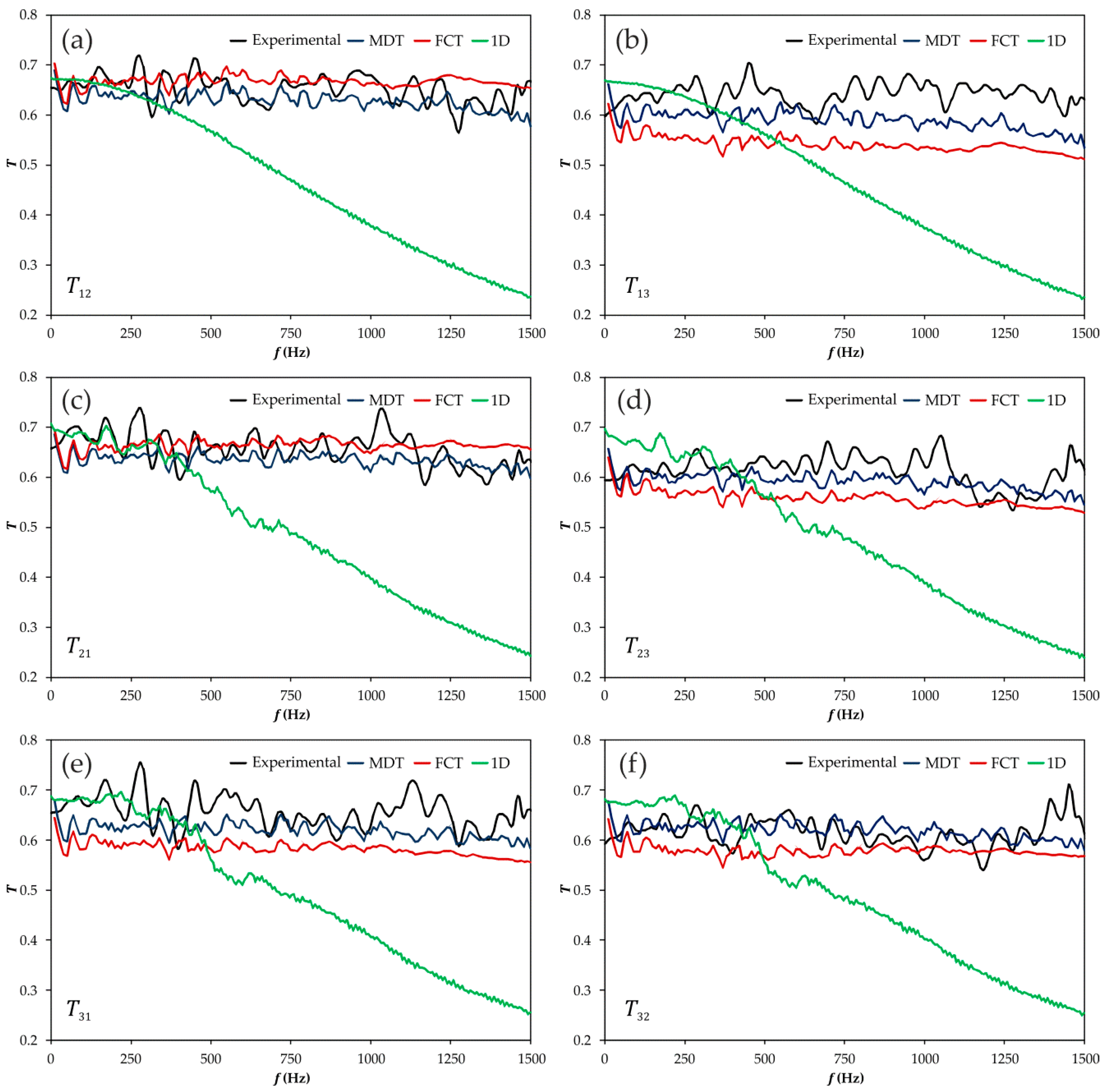
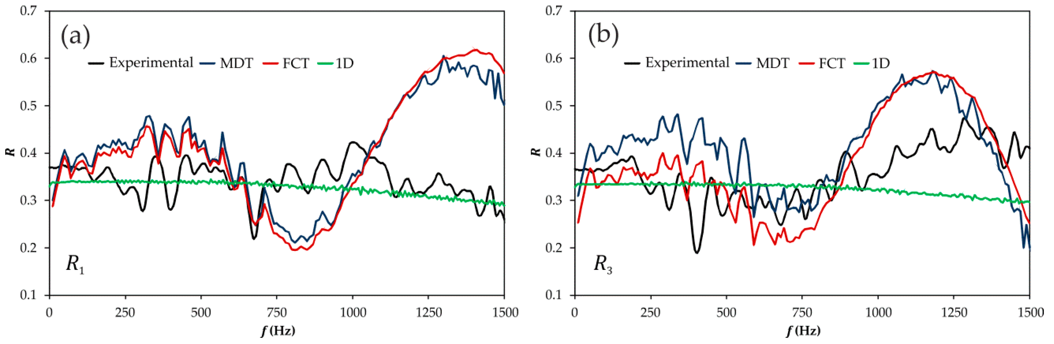
3.2.2. Frequency Domain Assessment

As already detected when describing the experimental results, it is in the frequency domain where the benefits of the staggered mesh finite volume method are more apparent. Consider first the results corresponding to the T-junction, shown in Figure 10 in the case of the reflection coefficients. Here, using either MDT or FCT as flux limiter, the staggered mesh finite volume method produces results for the reflection coefficients which overestimate dynamic effects when the excitation is at port 1, but produces a suitable approximation up to 1000 Hz when the excitation is at port 3 and the FCT flux limiter is used. In comparison with this, it is apparent that the conventional pressure loss model (again labeled as 1D in the figure) is unable to fully capture the dynamic features of the results, while still providing a sort of suitable average value, even if all the dynamic issues are lost, as an unavoidable consequence of the quasi-steady assumption underlying the calculation.
The corresponding transmission coefficients are shown in Figure 11, where it can be observed that the staggered mesh finite volume method produces results that follow the overall trend of the experimental results, with two exceptions: when the excitation is at port 1 the method underestimates the transmission to port 3, and when the excitation is at port 3 the method is unable to capture the behavior observed between 1000 and 1250 Hz. In the case of the conventional model, it is apparent that in this case it is fully unable to reproduce neither the level nor the dynamic features of the measured data, the only acceptable results being produced when the excitation is at port 1 and that only for very low frequencies.
This essential difference between the two modeling approaches considered is even more apparent in the case of the Y-junction, whose results are shown in Figure 12 and Figure 13 for the reflection and transmission coefficients, respectively. In this case, the results provided by the conventional model are rather similar regardless of the port at which the junction is excited. In all the cases, an acceptable value of the transmission coefficient in the very low frequencies is produced in those propagation paths with smaller change in direction, and also a suitable average value for the reflection coefficient as seen from any of the exciting ports. However, differences in transmission between the two propagation paths are not reproduced in any case and, moreover, the results start to decrease monotonically at about 200 Hz and reach totally unrealistic values for frequencies above 750 Hz in all the cases.
On the contrary, the staggered mesh finite volume method reproduces quite fairly the overall dependency with frequency, but tends to overestimate the influence of the change in direction of the propagation path on the transmission coefficients (and thus to underestimate the value of the corresponding coefficient). With this geometry, this effect is especially evident in the results obtained with the FCT flux limiter for | T 13 | , | T 23 | , | T 31 | and | T 32 | , i.e., all the cases in which the side branch (port 3) is involved. On the contrary, the results of the FCT method are affected by a certain overestimation when transmission through the main branch is considered ( | T 12 | and | T 21 | ). Accordingly, with the description given in Appendix B, this difference in behavior between the FCT and the MDT methods can only be due to the effect of the application to the junction itself of the different ways used to handle the information of the neighboring volumes when limiting the flow.
In the case of the reflection coefficients, the overestimation of the junction dynamics already observed in the T-junction is also present here when the junction is excited at port 1, but the measured dynamics are quite successfully reproduced when the junction is excited at ports 2 and 3. The characteristic frequencies governing the reflection coefficient are not exactly captured, but the overall amplitude and the influence of the exciting port are reproduced by the numerical results.

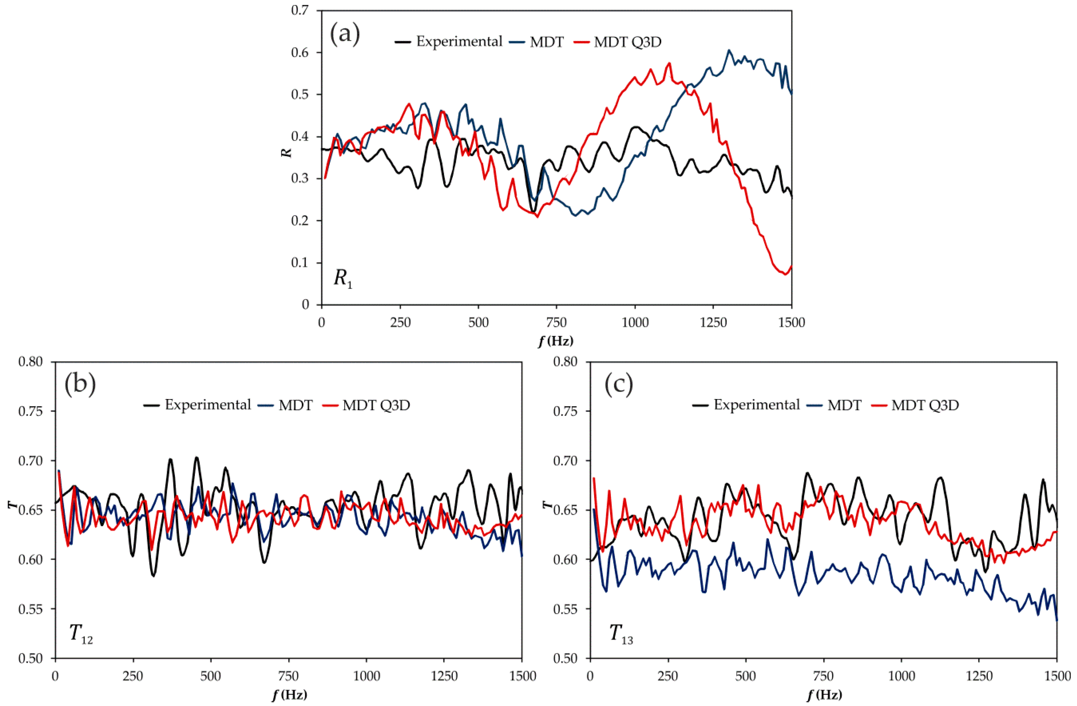
3.3. Assessment of a Modelling Approach with a Quasi-3D Description of the Junction

In order to explore the additional potential offered by the staggered mesh method regarding the approximate solution of the three-dimensional flow field inside the junction, such an approach (commonly referred to in the literature as quasi-3D) was finally considered. In Figure 14 the mesh used is shown together, for reference, with that used in the previous subsections. The four volumes at the endpoints of the part shown are then connected to a single volume, thus providing the connection with the one-dimensional computation at the ducts. The mesh chosen is relatively modest, in order to keep the computation time at reasonable values, but sufficient to show any potential advantages of this description.
Additionally, in view of the previous results, only the MDT method will be used as a flow limiter, since overall it has appeared to be more robust and consistent, and only the case of the T-junction will be analyzed in the following, as no new qualitative issues have been identified in the Y-junction that were not present also in the T-junction.

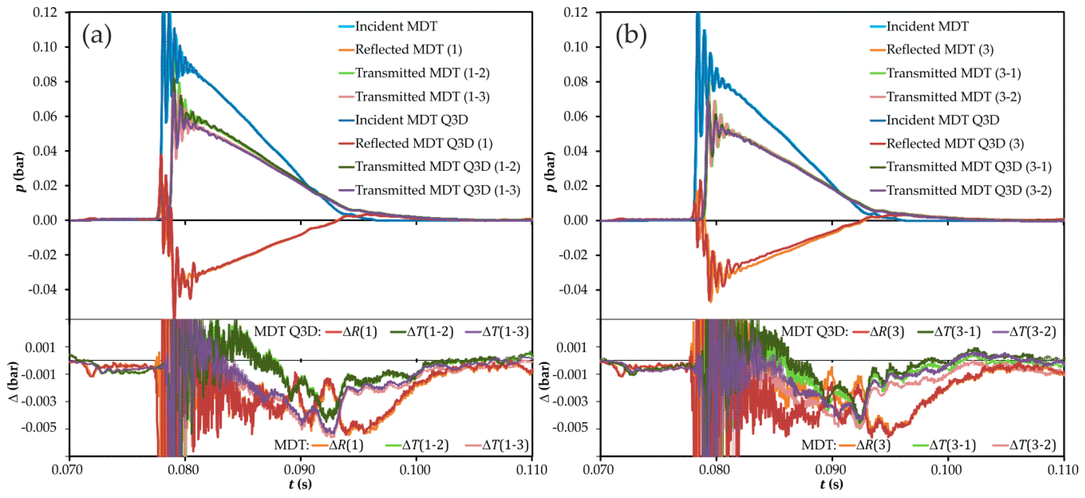
3.3.1. Time Domain Assessment

In Figure 15 the results obtained with the quasi-3D description of the junction (labeled MDT Q3D) are compared with those previously shown in Figure 7 corresponding to the MDT with 0D description of the junction. Again the plots on top represent the raw results, whereas the bottom plots show the differences with respect to the experimental values. It can be seen that, in all the cases, a certain improvement is achieved when using the quasi-3D junction, improvement which is more apparent when the junction is excited at port 3, this is, at the side branch, which is intuitively reasonable.
Again, the mean quadratic errors were computed, as shown in Table 3.
These results indicate that, while the reflection coefficients exhibit a similar mean error, there is a substantial improvement in the transmission coefficients, thus confirming the previous analysis.
However, the improvement achieved is not sufficient to produce results comparable to those shown in Figure 8 for the conventional model in the case of the reflection coefficient, and the differences in the transmission coefficients are clearly significant only when the junction is excited at the side branch. Therefore, while it appears that further refinement of the mesh at the junction should improve further the quality of the results, this might produce in turn an unacceptable increase in the computation time.

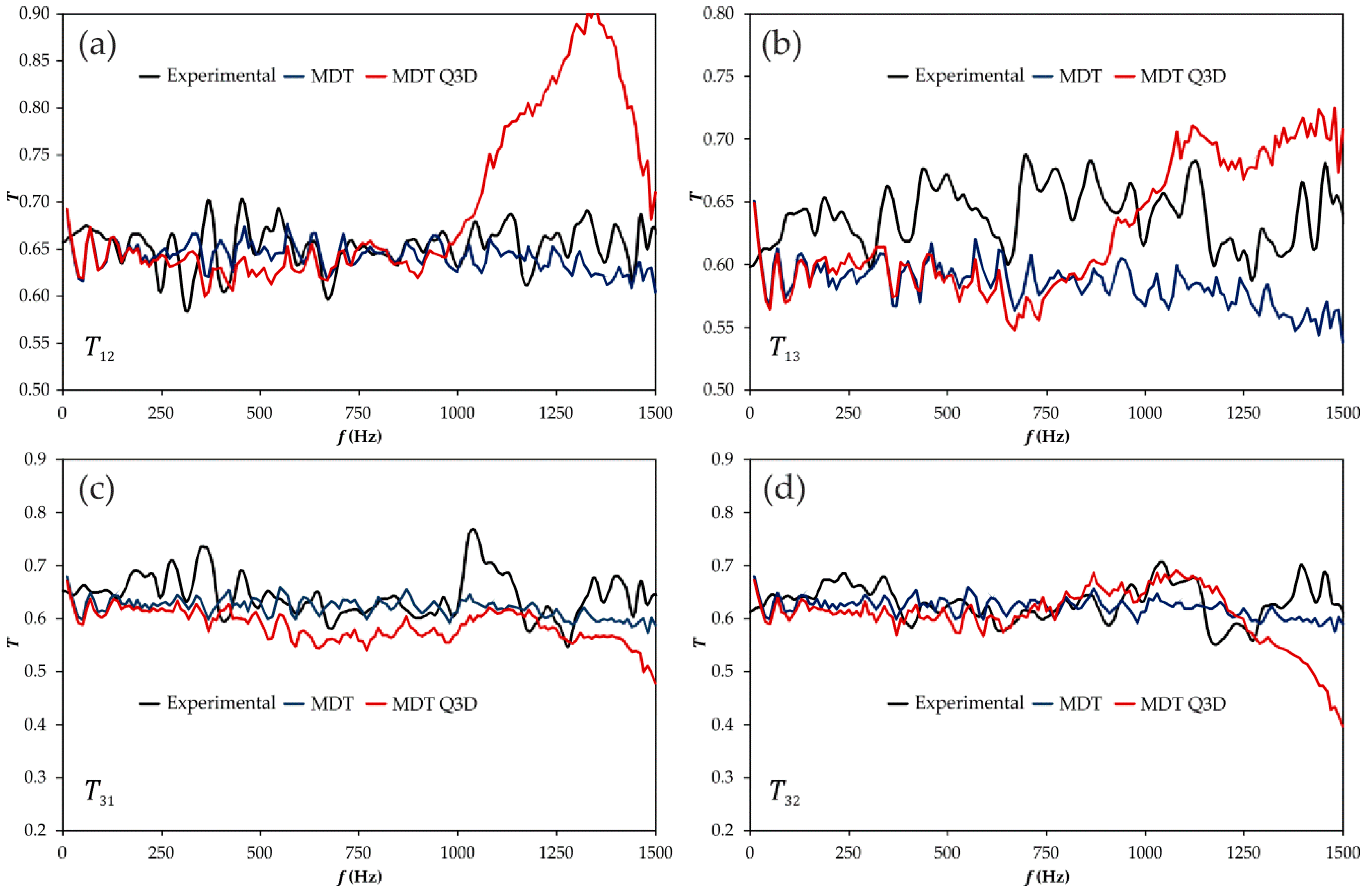
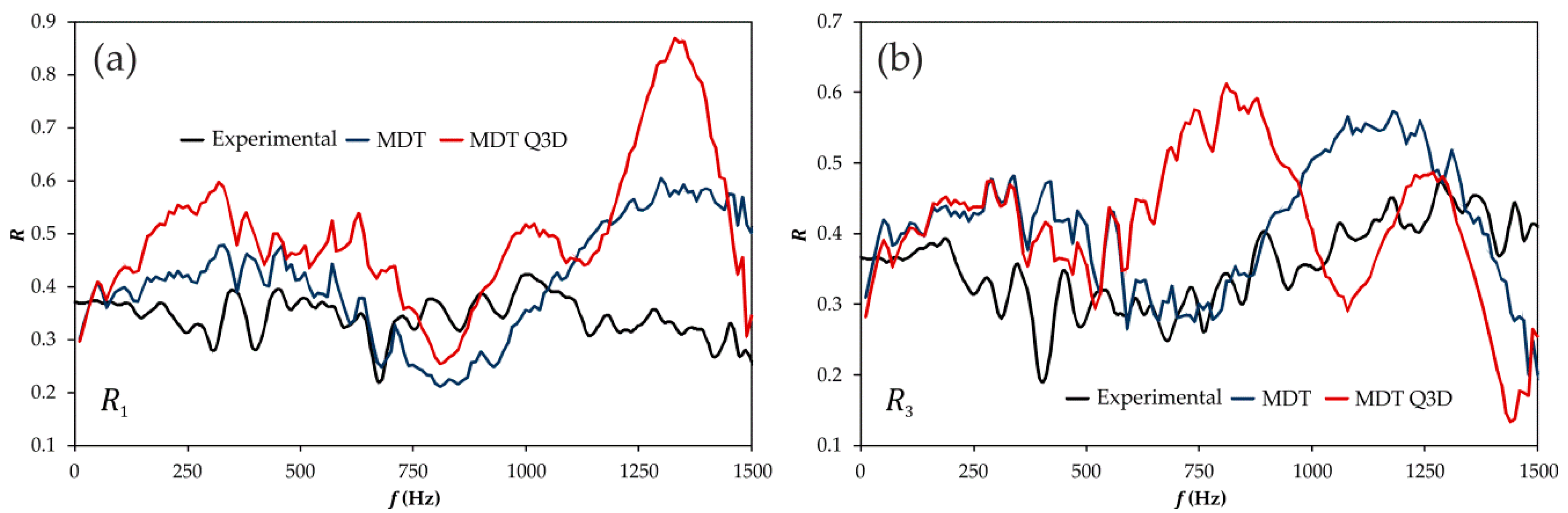
3.3.2. Frequency Domain Assessment

Quite unexpectedly, the improvements just commented do not have a translation in the frequency domain. In the case of the reflection coefficients, shown in Figure 16, the influence of the new description is apparent, but the new results do not provide any improvement in the reproduction of the experimental trend, showing even a certain degree of degradation in the quality of the results, with the abnormally high values achieved around 1300 Hz when the junction is excited at port 1.
The same comments apply to the transmission coefficients shown in Figure 17. The strange behavior around 1300 Hz is again present in those coefficients associated with the excitation at port 1, while when the junction is excited at port 3 no significant improvement can be detected.
The only possible explanation for the behavior observed, this is, something that produces minor but evident improvements in the time domain, but that induces a rather severe degradation in the quality of the results in the frequency domain, would be that some spurious high-frequency oscillations are being generated at the interface between the quasi-3D junction and the 1D elements of the adjacent ducts, due to the virtual merging of four volumes into a single one.
In order to clarify this point, the whole system was meshed as shown in Figure 14b for the junction, and the results are shown in Figure 18, only for the case in which the junction is excited at port 1. It is apparent that a dramatic improvement in the quality of the transmission coefficients is achieved, now showing a more realistic influence of the change in direction. In the case of the reflection coefficients the improvement is not so apparent, but the amplitude of the oscillations is smaller, what indicates that further refining of the mesh could lead to substantially improved results. However, that would be impractical, since the computation time increases substantially when the whole system is meshed in this way.

4. Conclusions

The objective of the work presented was to establish the potential of staggered mesh finite volume models as a way to improve the description of the effect of simple duct junctions on an otherwise one-dimensional flow system, as the intake or exhaust of an internal combustion engine.
With that purpose, specific experiments were performed making use of a modified impulse method, in which two different junctions were characterized as a multi-port, and that provided precise and reliable results on the propagation of pressure pulses across junctions.
The results obtained were then compared to numerical results obtained from different methods, both in the time and the frequency domains. First, methods assuming a zero-dimensional description of the junction were assessed, including the staggered mesh finite volume method with different flux limiters and, as a reference for comparison, a more conventional pressure loss-based model. Then, the potential of using the staggered mesh finite volume method in order to produce a quasi-3D description of the junction, to be coupled with the one-dimensional description of the adjacent ducts, was explored.
As an overall conclusion of the results found, one may state that none of the modeling approaches considered is able to reproduce totally the observed behavior. However, the performance of the different models is such that a suitable choice seems to be possible depending on which is the actual focus of the problem under study: situations in which a suitable time domain description may be sufficient may be addressed either with the conventional quasi-steady pressure loss model (most notably when the focus is on the reflection properties of the junction) or with the staggered mesh model with quasi-3D junction description (in this last case, when the main interest is on transmission, and given that the lengths involved in the problem will not be as long as to give rise to spurious oscillations due to the dispersive character of the method).
When the focus is on the frequency domain and on the dynamic behavior of the junction, it is the staggered mesh method the one that provides the most suitable results, at least from a qualitative point of view, as a consequence of the fact that momentum conservation across the junction is accounted for. However, due to spurious oscillation arising from the method used to couple a quasi-3D junction to the 1D ducts, suitable results with an acceptable computation time have been obtained only either with the zero-dimensional description of the junction or with a full quasi-3D description of the whole system, this last option being unacceptable in practice. It is thus clear that further work is needed in this case in order to find the optimal settings for the calculation, most notably in the connection between the quasi-3D and the 1D regions.
Finally, it should be recalled that no empirical information has been included in the staggered mesh method used; the incorporation of such information in terms of effective sections and characteristic lengths and the evaluation of their potential could be additional topics for further research.

Acknowledgments

Manuel Hernández is partially supported through contract FPI-S2-2015-1064 of Programa de Apoyo para la Investigación y Desarrollo (PAID) of Universitat Politècnica de València. The authors wish to thank Adolfo Guzmán for manufacturing the junctions and for his technical support during the tests.

Author Contributions

A.J. Torregrosa conceived the structure of the work, contributed to the analysis and wrote a large part of the article; A. Broatch supervised the experiments, wrote Appendix A and contributed to the discussion; L.M. García-Cuevas implemented the conventional model, ran the related simulations, wrote Appendix C and contributed to the discussion; M. Hernández implemented the staggered mesh method, ran the related simulations, wrote Appendix B and contributed largely to the discussion.

Conflicts of Interest

The authors declare no conflict of interest. The founding sponsors had no role in the design of the study; in the collection, analyses.

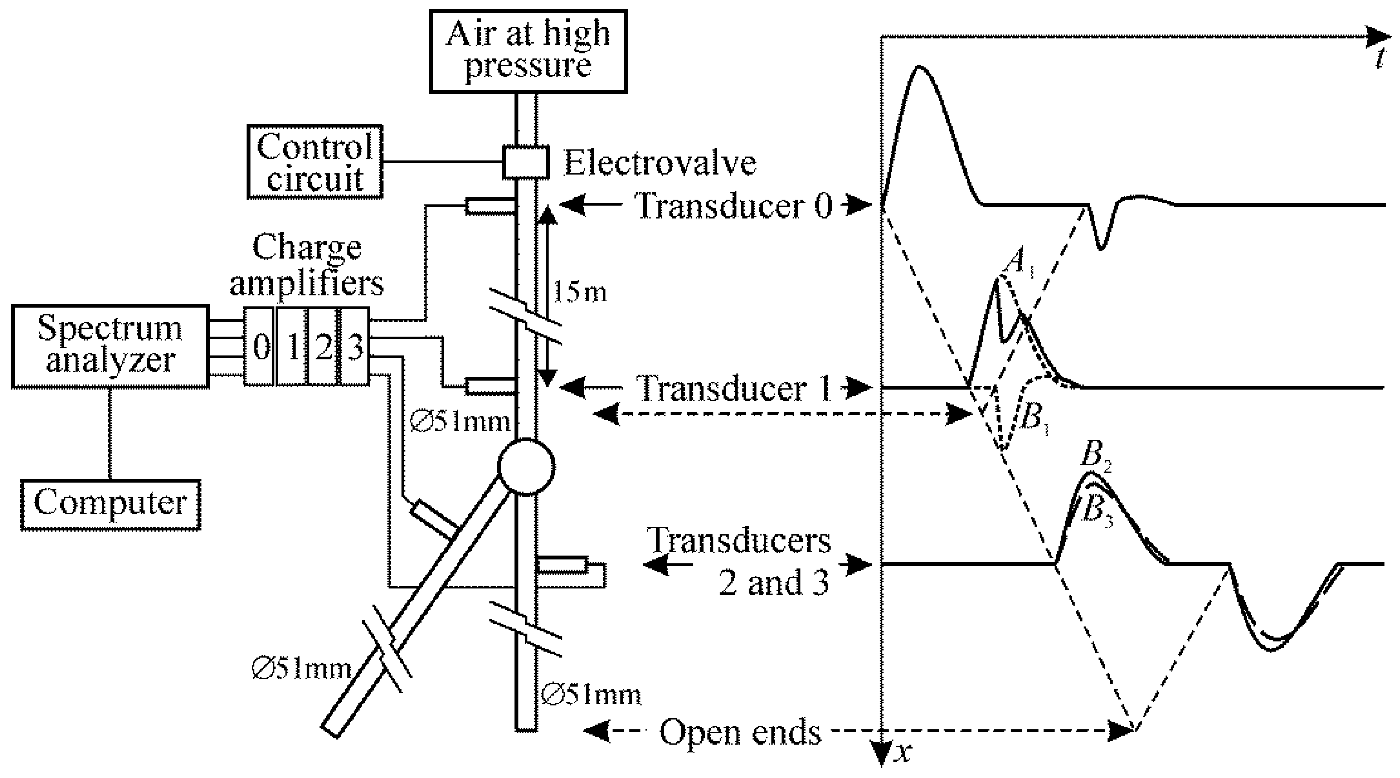
Appendix A. Experimental Procedure

Making reference to the notation in Figure 2, the determination of the transmission and reflection coefficients defined in Equation (1) requires the three following measurements:
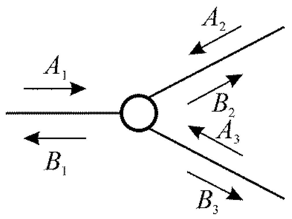
  • Excitation in duct 1, with anechoic terminations in ducts 2 and 3, so that A 1 0 and A 2 = A 3 = 0 , and thus,
    R 1 = B 1 / A 1 ;   T 12 = B 2 / A 1 ;   T 13 = B 3 / A 1   .
  • Excitation in duct 2, with anechoic terminations in ducts 1 and 3, so that A 2 0 and A 1 = A 3 = 0 ; then,
    R 2 = B 2 / A 2 ;   T 21 = B 1 / A 2 ;   T 23 = B 3 / A 2   .
  • Excitation in duct 3, with anechoic terminations in ducts 1 and 2, so that A 3 0 and A 1 = A 2 = 0 , so that,
    R 3 = B 3 / A 1 ;   T 31 = B 1 / A 3 ;   T 32 = B 2 / A 3   .
In order to perform the above-indicated tests, the modified version of the impulse method described in [28] was used, since pressure components, which all the previous developments are based upon, are directly obtained in the time domain with a simple procedure, and the consideration of three-port elements is straightforward. In Figure A1 both the experimental setup used and the relevant pressure waves recorded are illustrated.
Figure A1. Experimental setup used.
Applsci 07 00480 g019
The incident pulse is generated by means of a high speed electrovalve that controls the discharge from a high-pressure tank. A proper choice of the opening time ensures that the spectrum associated with the incident pulse is essentially flat. The length of the ducts placed between the valve and transducer 0, transducer 0 and the junction, and the junction and the open ends is chosen so that no windowing is necessary in order to isolate the incident, the reflected, and the transmitted pulses, as indicated in the figure. Transducer 0 was located 15 m away from both the valve and the junction, and transducers 2 and 3 were placed 0.15 m downstream of the junction, and 15 m away from their corresponding open end.
At the position indicated for transducer 1 in Figure 2, it is clear that this transducer records the addition of the incident and the reflected pulses, as illustrated in the figure. In order to surpass this difficulty, the solution adopted is to estimate the pulse incident on the junction at section 1 (whose Fourier transform will give the complex amplitude of the A 1 component) from an additional test performed without any element, using the pressure recorded by transducer 0 only to check the comparability of the excitations used in both types of tests (with and without junction).

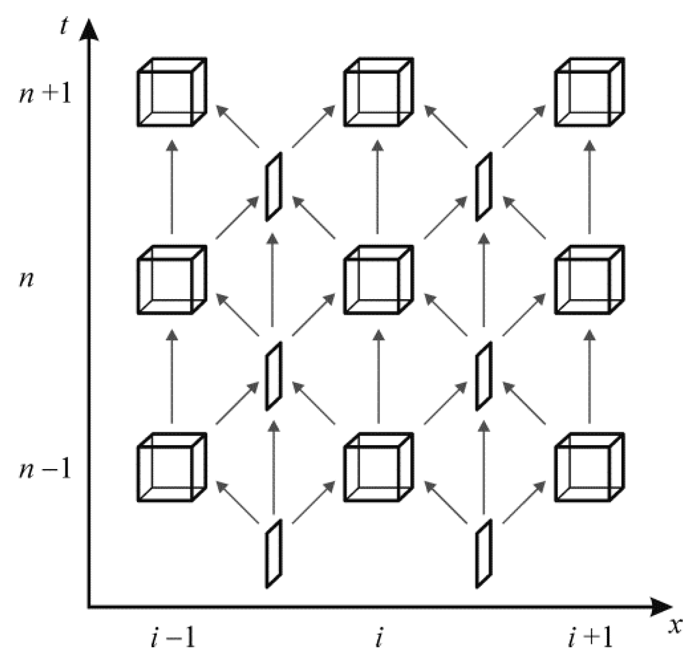
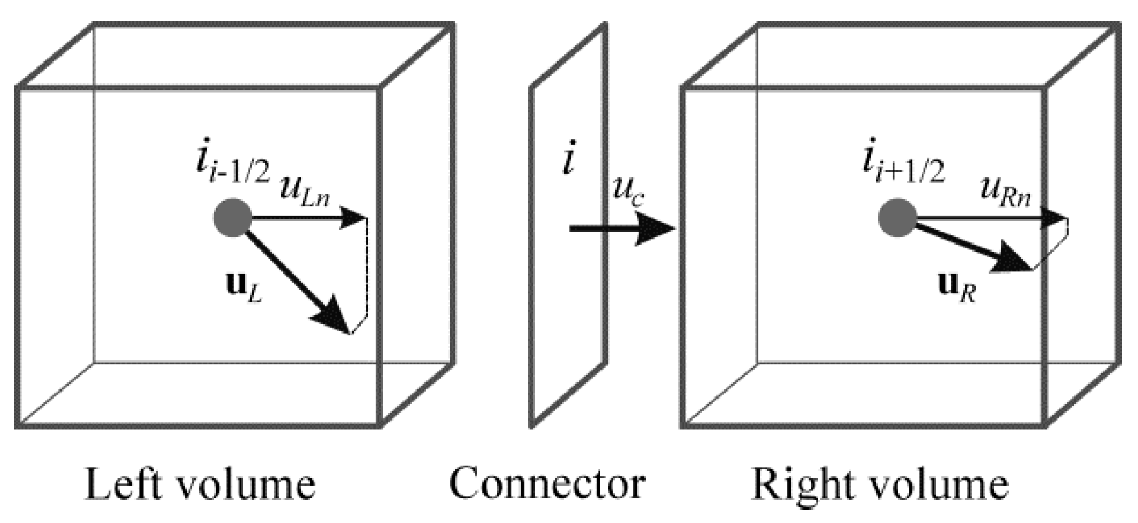
Appendix B. Staggered-Grid Finite-Volume Approach

As described by Torregrosa et al. [34], the quasi-3D model uses a staggered grid with two different basic elements: volumes and connectors. Volumes have associated scalar information such as pressure, density or temperature, as well as the cell volume. Connectors contain vector information, like flow velocity, momentum or the orientation of the connector in space, together with its area. With this configuration, a volume might have attached as many connectors as needed, but a connector will always connect only two volumes. In Figure A2 two volumes and a connector are shown schematically (volumes and connectors actually have an undefined shape).
Figure A2. Basic mesh elements, definition of velocity projections and notation of volumes and connectors.
Applsci 07 00480 g020
The method is based on the solution of the 3D Euler conservation equations without source term:
ρ / t + · ( ρ u ) = 0
( ρ u ) / t + · ( ρ uu ) = p
( ρ e 0 ) / t + · [ ( ρ e 0 + p ) u ] = 0
together with the perfect gas equation of state. Here, ρ is the density, p is the pressure, u is the velocity vector, · indicates the divergence, and e 0 is the specific stagnation internal energy, whose expression for a perfect gas is:
e 0 = c v T + u 2 / 2
where c v is the specific heat capacity at constant volume and T is the fluid static temperature.
However, in the context of a finite volume method on a staggered grid, the key issue is how and where these equations are solved. The mass conservation equation, being scalar, is solved in the volumes. Upon discretization it becomes:
ρ n + 1 = ρ n + Δ t V c = 1 N c ρ c n u c n A c
where u is the flow velocity. Superscript n indicates the time step, Δ t is the time interval, V the volume of the cell, N c the number of connectors, A is the cross section, and subscript c indicates that the variable is taken at a connector (otherwise it is assumed that the variable is taken at the volumes).
Following a similar procedure, the discretized energy equation is written as:
( ρ e 0 ) n + 1 = ( ρ e 0 ) n + Δ t V c = 1 N c ρ c n e 0 n u c n A c + Δ t V c = 1 N c p c n u c n A c
The momentum equation in a 3D case consists of three coupled equations. In this context, the momentum equation is solved in the connectors and only in the direction orthogonal to its surface. This is achieved by projecting the flow velocity of the two adjacent volumes into that direction, as shown in Figure A2, where the velocity u c in the connector, and the projections of the volume flow velocity from its left and right, u L n and u R n , are shown. As a result, the momentum in the connector follows a one-dimensional momentum equation, whose discretization gives:
( ρ c u c A c ) n + 1 = ( ρ c u c A c ) n + ( Δ t / Δ L ) [ ( ρ u n 2 + p ) L + ( ρ u n 2 + p ) R ] A c
Here, u n is the velocity projection onto the direction orthogonal to the connector surface and subscripts R and L denote the variables taken from the volumes at the right and left of the connector, respectively. With this simplification, a single equation is solved for each connector instead of three coupled equation for each volume. While usually the number of connectors is higher than the number of volumes in a 3D mesh, the fact that the momentum equations for each direction are not coupled reduces drastically the computation time when compared to a regular 3D method.
Once the momentum is calculated, its value is used to compute the mass and energy conservation equations in the next time step. It is worth noticing that some terms in the momentum and energy equations, like density or pressure, must be evaluated in the connectors, but are only calculated in the volumes. To solve this, an upwind approach is adopted, the required values being taken from the right or left volumes, depending on the flow direction.
Finally, the momentum in the volumes is computed by distributing the momentum calculated in the connectors among the volumes they connect, taking into account their size. In a uniform 1D mesh, half the momentum is thus assigned to each volume. As the orientation of the connectors in space is known, the resulting momentum vector of a volume can be calculated from the vector sum of the momentum in the connectors:
( ρ c u V ) v n + 1 = 1 2 c = 1 N c ( ρ u c A c Δ L ) c n + 1
The resulting method is a second-order accuracy method based on an explicit scheme with a staggered grid, as shown in Figure A3.
Figure A3. Scheme of the staggered mesh and the associated time marching.
Applsci 07 00480 g021
The fact that the resulting scheme offers second-order accuracy, together with the simplifications adopted in the momentum equation, results in nonphysical oscillations, especially in the vicinity of significant pressure gradients. In order to mitigate such overshoots, two different flux limiters have been used here: the momentum diffusion term (MDT) proposed in [35] and the flux-corrected transport (FCT) methodology proposed in [34].
In the case of the MDT, the main goal is to add a diffusion term to the momentum equation so that the mass flux computed at that connector is conveniently limited. With this purpose, the momentum flux density tensor used in the momentum Equation (A5) can be modified, in a way similar to that used for incorporating viscosity effects, as follows:
( ρ u ) / t + · ( ρ uu + D ) = p
where the tensor D is assumed to depend linearly on the local momentum gradients, i.e.,
D = ϵ ( ρ u )
The scalar quantity ϵ has the dimensions of a kinematic viscosity and can thus be interpreted as a momentum diffusion coefficient. With this prescription, the contribution of the diffusion term · D will only be relevant if significant gradients exist, and any resulting spurious oscillations will be damped.
Adding the projection of Equation (A12) onto the direction of a connector to the discretized momentum equation one gets:
( ρ c u c A c ) n + 1 = ( ρ c u c A c ) n + ( Δ t Δ L ) { [ ( ρ u n 2 + p ) L + ( ρ u n 2 + p ) R ] A c + ( D ˜ L n D ˜ R n ) }
where D ˜ L and D ˜ R are the projections onto the connector direction of tensor D ˜ = ϵ ( ρ u A ) computed in the two adjacent volumes. Following [35], the momentum diffusion coefficient is computed by relating the mesh size and the time step to the local flow velocity at the volume, as:
ϵ = | u | 2 ( Δ L | u | Δ t )
and the gradient of mass flow ( ρ u A ) is also computed from the projections of the mass flows of the adjacent connectors onto each direction.
Considering now the FCT technique, it was initially conceived to be used in a finite differences scheme, but it was adapted to a finite volume staggered grid in [34]. In the FCT technique three stages can be identified: a transport stage based on the scheme considered, a diffusion stage where the numerical dispersion is reduced, and an anti-diffusion stage in which the accuracy of the scheme where the solution is smooth is restored. The diffusion operator is defined as:
D j ( W ) = θ ( W j + 1 / 2 ) θ ( W j 1 / 2 )
with,
θ ( W j + 1 / 2 ) = ϑ / 4 ( W j + 1 W j )
where W j is the conservative variable computed at cell j in the transport stage, j ± 1 / 2 indicates that the conservative variable is evaluated in the midpoint between j and j ± 1 , and the factor ϑ is a positive real number with ϑ 1 / 2 . Calculating the diffusion via damping, as suggested in [34], the new variable W ¯ j is obtained as:
W ¯ j n + 1 = W j n + 1 + D j ( W n )
When considering a staggered mesh finite volume method, the FCT is only applied to the momentum equation, since this is the main source of oscillations. Therefore, all the calculations in the volumes are made using W j n = ( ρ u c A c ) j n as the conservative variable, whereas the calculations in the midpoints make use of the variables evaluated at the volumes adjacent to the connector.
Finally, the non-linear anti-diffusion operator A j is defined as:
A j ( W ) = Ψ ( W j 1 / 2 ) Ψ ( W j + 1 / 2 )
Making use of the anti-diffusive limited flow defined in [37] gives:
Ψ ( W j + 1 / 2 ) = s max [ 0 , min ( ( 5 / 8 ) s   Δ W j 1 / 2 , ( 1 / 8 ) | Δ W j + 1 / 2 | , ( 5 / 8 ) s   Δ W j + 3 / 2 ) ]
where s   =   sign ( Δ W j 1 / 2 ) ,   Δ W j 1 / 2 = W j W j 1 ,   Δ W j + 1 / 2 = W j + 1 W j and Δ W j + 3 / 2 = W j + 2 W j + 1 . Then, according to [34], the phoenical form should be used, so that:
W = j n + 1 = W ¯ j n + 1 + A j ( W n + 1 )
The anti-diffusion stage equations can be adapted to the staggered grid mesh finite volume method in a way similar to that used with the diffusion stage.

Appendix C. 1D Method with Pressure Loss-Based Junction Model

In this case, a collocated one-dimensional finite volume method is used for all the calculations inside the pipes. The Euler equations of fluid dynamics simplified for one-dimensional flow in a straight uniform duct can be expressed as:
d W ¯ i d t = d d t ( ρ ρ u ρ e 0 ) i = A ( F i 1 , i F i , i + 1 ) V i
Here, W ¯ i is the cell-averaged state vector of cell i,   F i 1 , i and F i , i + 1 are the inter-cell fluxes between cells i 1 and i and between i and i + 1 , respectively, and the other symbols refer to the same magnitudes as in Appendix B, with u being now the axial velocity of the flow. The inter-cell fluxes are computed by an approximate solution of the Riemann problem as described by Toro et al. [38]. The state vector is extrapolated to the cell boundaries to compute the fluxes by means of a Monotonic Upstream-Centered Scheme for Conservation Laws (MUSCL) approach as described in [39], while the solution is propagated in time using Heun’s method, leading to a second order in time and space, total variation diminishing scheme.
While the main one-dimensional flow inside the ducts is simulated, the effects of the geometry of the junction are modelled. The connections of the ducts to the junction are solved using an auxiliary small zero-dimensional element. Each of the one-dimensional branches is connected to that zero-dimensional element making use of the Riemann variables to compute the fluxes at their corresponding boundary. At each connection, it is assumed that a certain amount of stagnation pressure is lost, depending on the angle of the junction and of the ratio between the outflow mass flow m ˙ o u t passing through the branch of interest and the inflow mass flow m ˙ i n . The pressure loss coefficients are computed following the expressions given in [15,16], and are defined as the ratio of the difference in stagnation pressure between the outflow branch and the inflow branch to the dynamic pressure ( ρ u 2 / 2 ) of the inflow branch. Finally, the total pressure loss coefficient K for a three-branch junction with the same section in all the branches can be estimated as:
K = ( m ˙ o u t m ˙ i n ) 2 3 2 m ˙ o u t m ˙ i n + 1 2
when the branch is collinear with the inflow branch, and,
K = ( m ˙ o u t m ˙ i n ) 2 + 1 2 m ˙ o u t m ˙ i n cos ( 3 4 θ )
for the lateral branch, when the flow is split between a collinear and a lateral branch. In this case, θ is the angle between the lateral branch and the axial outflow branch, so that 0° means that both outflow branches are parallel. The same expression applies when the inflow branch is not parallel to any of the outflow branches: in that case, the angle θ is measured between the inflow branch and the other outflow branch.
In the auxiliary zero-dimensional element, the gas is again considered as a perfect gas, and the mass and energy equations are solved:
d m d t = m ˙
d ( m c v T ) d t = m ˙ h 0
where m is the mass trapped in the zero-dimensional element, m ˙ is the mass flow, positive when it enters the element, and h 0 is the specific stagnation enthalpy associated with the mass moving inside or outside of the element. These two equations set an additional limitation to the maximum possible time step.

References

  1. Winterbone, D.E.; Pearson, R.J. Design Techniques for Engine Manifolds, 3rd ed.; Professional Engineering Pub. Ltd.: London, UK, 1999. [Google Scholar]
  2. Payri, F.; Reyes, E.; Galindo, J. Analysis and modelling of the fluid-dynamic effects in branched exhaust junctions of I.C.E. J. Eng. Gas Turbines Power 2001, 123, 197–203. [Google Scholar] [CrossRef]
  3. Tang, S.K. Sound transmission characteristics of Tee-junctions and the associated length corrections. J. Acoust. Soc. Am. 2004, 115, 218–227. [Google Scholar] [CrossRef] [PubMed]
  4. Harrison, M.F.; De Soto, I.; Rubio-Unzueta, P.L. A linear acoustic model for multi-cylinder IC engine intake manifolds including the effects of the intake throttle. J. Sound Vib. 2004, 278, 975–1011. [Google Scholar] [CrossRef]
  5. Karlsson, M.; Abom, M. Quasi-steady model of the acoustic scattering properties of a T-junction. J. Sound Vib. 2011, 330, 5131–5137. [Google Scholar] [CrossRef]
  6. Karlsson, M.; Abom, M. Aeroacoustics of T-junctions—An experimental investigation. J. Sound Vib. 2010, 329, 1793–1808. [Google Scholar] [CrossRef]
  7. Desantes, J.M.; Torregrosa, A.J.; Broatch, A. Experiments on flow noise generation in simple exhaust geometries. Acta Acust. United Acust. 2001, 87, 46–55. [Google Scholar]
  8. Benson, R.S. The Thermodynamics and Gas Dynamics of Internal-Combustion Engines; Clarendon Press: Oxford, UK, 1982; Volume 1. [Google Scholar]
  9. Corberán, J.M. A new constant pressure model for N-branch junctions. Proc. Inst. Mech. Eng. D 1992, 206, 117–123. [Google Scholar] [CrossRef]
  10. Schmandt, B.; Herwig, H. The head change coefficient for branched flows: Why ‘‘losses’’ due to junctions can be negative. Int. J. Heat Fluid Flow 2015, 54, 268–275. [Google Scholar] [CrossRef]
  11. Shaw, C.T.; Lee, D.J.; Richardson, S.H.; Pierson, S. Modelling the effect of plenum-runner interface geometry on the flow through an inlet system. SAE Tech. Pap. Ser. 2000. [Google Scholar] [CrossRef]
  12. Pérez-García, J.; Sanmiguel-Rojas, E.; Hernández-Grau, J.; Viedma, A. Numerical and experimental investigations on internal compressible flow at T-type junctions. Exp. Therm. Fluid Sci. 2006, 31, 61–74. [Google Scholar] [CrossRef]
  13. Naeimi, H.; Domiry Ganji, D.; Gorji, M.; Javadirad, G.; Keshavarz, M. A parametric design of compact exhaust manifold junction in heavy duty diesel engine using computational fluid dynamics codes. Therm. Sci. 2011, 15, 1023–1033. [Google Scholar] [CrossRef]
  14. Sakowitz, A.; Mihaescu, M.; Fuchs, L. Turbulent flow mechanisms in mixing T-junctions by Large Eddy Simulations. Int. J. Heat Fluid Flow 2014, 45, 135–146. [Google Scholar] [CrossRef]
  15. Bassett, M.D.; Winterbone, D.E.; Pearson, R.J. Calculation of steady flow pressure loss coefficients for pipe junctions. Proc. Inst. Mech. Eng. C 2001, 215, 861–881. [Google Scholar] [CrossRef]
  16. Hager, W.H. An approximate treatment of flow in branches and bends. Proc. Inst. Mech. Eng. C 1984, 198, 63–69. [Google Scholar] [CrossRef]
  17. Paul, J.; Selamet, A.; Miazgowicz, K.D.; Tallio, K.V. Combining flow losses at circular T-junctions representative of intake plenum and primary runner interface. SAE Tech. Pap. Ser. 2007. [Google Scholar] [CrossRef]
  18. Pérez-García, J.; Sanmiguel-Rojas, E.; Viedma, A. New coefficient to characterize energy losses in compressible flow at T-junctions. Appl. Math Model. 2010, 34, 4289–4305. [Google Scholar] [CrossRef]
  19. Wang, W.; Lu, Z.; Deng, K.; Qu, S. An experimental study of compressible combining flow at 45° T-junctions. Proc. Inst. Mech. Eng. C 2015, 229, 1600–1610. [Google Scholar] [CrossRef]
  20. Peters, B.; Gosman, A.D. Numerical simulation of unsteady flow in engine intake manifolds. SAE Tech. Pap. Ser. 1993. [Google Scholar] [CrossRef]
  21. Bingham, J.F.; Blair, G.P. An improved branched pipe model for multi-cylinder automotive engine calculations. Proc. Inst. Mech. Eng. Part D 1985, 199, 65–77. [Google Scholar] [CrossRef]
  22. William-Louis, M.J.P.; Ould-El-Hadrami, A.; Tournier, C. On the calculation of the unsteady compressible flow through an N-branch junction. Proc. Inst. Mech. Eng. C 1998, 212, 49–56. [Google Scholar] [CrossRef]
  23. Bassett, M.D.; Pearson, R.J.; Fleming, N.P.; Winterbone, D.E. A multi-pipe junction model for one-dimensional gas-dynamic simulations. SAE Tech. Pap. Ser. 2003. [Google Scholar] [CrossRef]
  24. Pearson, R.J.; Bassett, M.D.; Batten, P.; Winterbone, D.E.; Weaver, N.W.E. Multi-dimensional wave propagation in pipe junctions. SAE Tech. Pap. Ser. 1999. [Google Scholar] [CrossRef]
  25. Bassett, M.D.; Winterbone, D.E.; Pearson, R.J. Modelling engines with pulse converted exhaust manifolds using one-dimensional techniques. SAE Tech. Pap. Ser. 2000. [Google Scholar] [CrossRef]
  26. Montenegro, G.; Onorati, A.; Piscaglia, F.; D’Errico, G. Integrated 1D-multiD fluid dynamic models for the simulation of I.C.E. intake and exhaust systems. SAE Tech. Pap. Ser. 2007. [Google Scholar] [CrossRef]
  27. Onorati, A.; Montenegro, G.; D’Errico, G.; Piscaglia, F. Integrated 1D-3D fluid dynamic simulation of a turbocharged Diesel engine with complete intake and exhaust systems. SAE Tech. Pap. Ser. 2010. [Google Scholar] [CrossRef]
  28. Montenegro, G.; Onorati, A.; Della Torre, A. The prediction of silencer acoustical performances by 1D, 1D-3D and quasi-3D non-linear approaches. Comput. Fluids 2013, 71, 208–223. [Google Scholar] [CrossRef]
  29. Morel, T.; Silvestri, J.; Goerg, K.; Jebasinski, R. Modeling of engine exhaust acoustics. SAE Tech. Pap. Ser. 1999. [Google Scholar] [CrossRef]
  30. Sapsford, S.M.; Richards, V.C.M.; Amlee, D.R.; Morel, T.; Chappell, M.T. Exhaust system evaluation and design by non-linear modeling. SAE Tech. Pap. Ser. 1992. [Google Scholar] [CrossRef]
  31. Montenegro, G.; Della Torre, A.; Onorati, A.; Fairbrother, R.; Dolinar, A. Development and application of 3D generic cells to the acoustic modelling of exhaust systems. SAE Tech. Pap. Ser. 2011. [Google Scholar] [CrossRef]
  32. Payri, F.; Desantes, J.M.; Broatch, A. Modified impulse method for the measurement of the frequency response of acoustic filters to weakly nonlinear transient excitations. J. Acoust. Soc. Am. 2000, 107, 731–738. [Google Scholar] [CrossRef] [PubMed]
  33. Torregrosa, A.J.; Broatch, A.; Fernández, T.; Denia, F.D. Description and measurement of the acoustic characteristics of two-tailpipe mufflers. J. Acoust. Soc. Am. 2006, 119, 723–728. [Google Scholar] [CrossRef]
  34. Torregrosa, A.J.; Broatch, A.; Arnau, F.J.; Hernández, M. A non-linear quasi-3D model with Flux- Corrected-Transport for engine gas-exchange modelling. J. Comput. Appl. Math. 2016, 291, 103–111. [Google Scholar] [CrossRef]
  35. Montenegro, G.; Della Torre, A.; Onorati, A.; Fairbrother, R. Nonlinear quasi-3D approach for the modeling of mufflers with perforated elements and sound-absorbing material. Adv. Acoust. Vib. 2013, 2013, 546120. [Google Scholar] [CrossRef]
  36. OpenWAM. CMT—Motores Térmicos, Universitat Politècnica de València. Available online: http://www.openwam.org/ (accessed on 20 March 2017).
  37. Ikeda, T.; Nakagawa, T. On the SHASTA FCT algorithm for the equation ∂ρ/∂t+(∂/∂x)(v(ρ)ρ)=0. Math. Comput. 1979, 33, 1157–1169. [Google Scholar] [CrossRef]
  38. Toro, E.F.; Spruce, M.; Speares, W. Restoration of the contact surface in the HLL-Riemann solver. Shock Waves 1994, 4, 25–34. [Google Scholar] [CrossRef]
  39. Van Leer, B. Towards the ultimate conservative difference scheme. V. A second-order sequel to Godunov’s method. J. Comput. Phys. 1979, 32, 101–136. [Google Scholar] [CrossRef]
Figure 1. Junctions considered in the study.
Applsci 07 00480 g001
Figure 2. Wave components acting on a multi-port.
Applsci 07 00480 g002
Figure 3. Experimental results for the T-junction in the time domain. (a) Excitation at port 1; (b) excitation at port 3. Ports are denoted as in Figure 1.
Applsci 07 00480 g003
Figure 4. Experimental results for the Y-junction in the time domain. (a) Excitation at port 1; (b) excitation at port 2; (c) excitation at port 3. Ports are denoted as in Figure 1.
Applsci 07 00480 g004
Figure 5. Experimental results for the T-junction in the frequency domain. (a) Excitation at port 1; (b) excitation at port 3. Ports are denoted as in Figure 1. R i : reflection coefficient as seen from port i ; T i j : transmission coefficient between ports i and j .
Applsci 07 00480 g005
Figure 6. Experimental results for the Y-junction in the frequency domain. (a) Excitation at port 1; (b) excitation at port 2; (c) excitation at port 3. Ports are denoted as in Figure 1. R i : reflection coefficient as seen from port i ; T i j : transmission coefficient between ports i and j .
Applsci 07 00480 g006
Figure 7. Experimental vs. modeled results for the T-junction: raw data (top) and differences (bottom) in the time domain, momentum diffusion term (MDT) method. (a) excitation at port 1; (b) excitation at port 3. Ports are denoted as in Figure 1. Δ R ( i ) : difference in the pulse reflected at port i ; Δ T ( i j ) : difference in the pulse transmitted between ports i and j .
Applsci 07 00480 g007
Figure 8. Comparison between the different models for the T-junction: raw data (top) and differences (bottom plots) in the time domain. (a) excitation at port 1; (b) excitation at port 3. Ports are denoted as in Figure 1. Δ R ( i ) : difference in the pulse reflected at port i ; Δ T ( i j ) : difference in the pulse transmitted between ports i and j . FCT: flux-corrected transport; MDT: momentum diffusion term; 1D: conventional pressure-loss model.
Applsci 07 00480 g008
Figure 9. Comparison between the different models considered for the Y-junction (time domain): (a) excitation at port 1; (b) excitation at port 2; (c) excitation at port 3. Ports are denoted as in Figure 1. Δ R ( i ) : difference in the pulse reflected at port i ; Δ T ( i j ) : difference in the pulse transmitted between ports i and j . FCT: flux-corrected transport; MDT: momentum diffusion term; 1D: conventional pressure-loss model.
Applsci 07 00480 g009
Figure 10. Comparison between the experimental results and the different models for the reflection coefficients of the T-junction (frequency domain): (a) excitation at port 1; (b) excitation at port 3. Ports are denoted as in Figure 1.
Applsci 07 00480 g010
Figure 11. Comparison between the experimental results and the different models for the transmission coefficients of the T-junction (frequency domain): (a) excitation at port 1, transmission through port 2; (b) excitation at port 1, transmission through port 3; (c) excitation at port 3, transmission through port 1; (d) excitation at port 3, transmission through port 2. Ports are denoted as in Figure 1.
Applsci 07 00480 g011
Figure 12. Comparison between the experimental results and the different models for the reflection coefficients of the Y-junction (frequency domain): (a) excitation at port 1; (b) excitation at port 2; (c) excitation at port 3. Ports are denoted as in Figure 1.
Applsci 07 00480 g012aApplsci 07 00480 g012b
Figure 13. Comparison between the experimental results and the different models for the transmission coefficients of the Y-junction (frequency domain): (a) excitation at port 1, transmission through port 2; (b) excitation at port 1, transmission through port 3; (c) excitation at port 2, transmission through port 1; (d) excitation at port 2, transmission through port 3 (e) excitation at port 3, transmission through port 1; (f) excitation at port 3, transmission through port 2. Ports are denoted as in Figure 1.
Applsci 07 00480 g013
Figure 14. Meshes used in the staggered-grid method: (a) a 0D description of the junction; (b) a quasi-3D description.
Applsci 07 00480 g014
Figure 15. Influence of the description of the junction in the time domain, MDT method: raw data (top) and differences with measurement (bottom). (a) Excitation at port 1; (b) excitation at port 3. Ports are denoted as in Figure 1.
Applsci 07 00480 g015
Figure 16. Influence of the description of the junction on the reflection coefficients (frequency domain), MDT method. (a) Excitation at port 1; (b) excitation at port 3. Ports are denoted as in Figure 1.
Applsci 07 00480 g016
Figure 17. Influence of the description of the junction on the reflection coefficients (frequency domain), MDT method. (a) excitation at port 1, transmission through port 2; (b) excitation at port 1, transmission through port 3; (c) excitation at port 3, transmission through port 1; (d) excitation at port 3, transmission through port 2. Ports are denoted as in Figure 1.
Applsci 07 00480 g017
Figure 18. Influence of using a quasi-3D approach for the whole system on the reflection and transmission coefficients (frequency domain). MDT method, excitation at port 1. (a) reflection at port 1; (b) transmission through port 2; (c) transmission through port 3. Ports are denoted as in Figure 1.
Applsci 07 00480 g018
Table 1. Values of the mean quadratic error: T-junction.
PathMDTFCT1D
R(1)1.514 × 10−41.842 × 10−41.448 × 10⁻⁴
R(3)1.102 × 10−42.046 × 10−41.019 × 10⁻⁴
T(1–2)1.005 × 10−49.932 × 10−56.926 × 10⁻⁵
T(1–3)1.609 × 10−41.298 × 10−41.774 × 10⁻⁴
T(3–1)1.121 × 10−41.094 × 10−41.114 × 10⁻⁴
T(3–2)1.554 × 10−41.245 × 10−41.833 × 10⁻⁴
Abbreviations: FCT: flux-corrected transport; MDT: momentum diffusion term; 1D: conventional pressure-loss model.
Table 2. Values of the mean quadratic error: Y-junction.
PathMDTFCT1D
R(1)1.575 × 10−41.915 × 10−41.273 × 10⁻⁴
R(2)1.992 × 10−42.172 × 10−41.681 × 10⁻⁴
R(3)1.648 × 10−42.945 × 10−41.394 × 10⁻⁴
T(1–2)1.171 × 10−41.369 × 10−49.186 × 10⁻⁵
T(1–3)1.514 × 10−41.322 × 10−41.742 × 10⁻⁴
T(2–1)1.992 × 10−42.172 × 10−41.681 × 10⁻⁴
T(2–3)1.336 × 10−41.296 × 10−41.141 × 10⁻⁴
T(3–1)1.669 × 10−41.949 × 10−41.355 × 10⁻⁴
T(3–2)2.117 × 10−41.516 × 10−41.751 × 10⁻⁴
Abbreviations: FCT: flux-corrected transport; MDT: momentum diffusion term; 1D: conventional pressure-loss model.
Table 3. Values of the mean quadratic error: T-junction.
PathMDTMDT Q3D
R(1)1.514 × 10−41.513 × 10−4
R(3)1.102 × 10−41.809 × 10−4
T(1–2)1.005 × 10−41.018 × 10−4
T(1–3)1.609 × 10−41.469 × 10−4
T(3–1)1.121 × 10−41.044 × 10−4
T(3–2)1.554 × 10−41.249 × 10−4
Abbreviations: MDT Q3D: momentum diffusion term with quasi-3D description of the junction.

