Uniaxial Compressive Strength and Fracture Mode of Lake Ice at Moderate Strain Rates Based on a Digital Speckle Correlation Method for Deformation Measurement

Abstract

Better understanding of the complex mechanical properties of ice is the foundation to predict the ice fail process and avoid potential ice threats. In the present study, uniaxial compressive strength and fracture mode of natural lake ice are investigated over moderate strain-rate range of 0.4–10 s⁻¹ at −5 °C and −10 °C. The digital speckle correlation method (DSCM) is used for deformation measurement through constructing artificial speckle on ice sample surface in advance, and two dynamic load cells are employed to measure the dynamic load for monitoring the equilibrium of two ends’ forces under high-speed loading. The relationships between uniaxial compressive strength and strain-rate, temperature, loading direction, and air porosity are investigated, and the fracture mode of ice at moderate rates is also discussed. The experimental results show that there exists a significant difference between true strain-rate and nominal strain-rate derived from actuator displacement under dynamic loading conditions. Over the employed strain-rate range, the dynamic uniaxial compressive strength of lake ice shows positive strain-rate sensitivity and decreases with increasing temperature. Ice obtains greater strength values when it is with lower air porosity and loaded vertically. The fracture mode of ice seems to be a combination of splitting failure and crushing failure.

1. Introduction

Many engineering fields, such as ocean and river transportation in cold regions, energy exploration and exploitation in freezing territorial waters, and aviation and spaceflight, involve ice mechanics. Better understanding of the complex mechanical properties of ice is the foundation to predict the ice failure process and avoid potential ice threats. Many researchers have conducted extensive experiments to investigate the mechanical properties of freshwater ice, sea ice, and artificial ice under creep and quasi-static conditions; relationships between compressive strength and strain-rate, temperature, loading direction, and the internal structure of ice have been obtained [1,2,3,4]. In the past ten years, many researchers have started to investigate ice mechanical behavior at high strain rates in the magnitude range of hundreds and thousands by use of split Hopkinson pressure bar (SPBH) or a high-speed jack, accompanying with a high-speed camera, and several experiments [5,6,7,8,9,10,11,12,13] have been carried out, as there is a need for high-speed impact behavior of ice in a broad range of engineering areas. Study of ice mechanics extends from low strain rates to moderate and high strain rates.

Both Jones [5] and Meglis and Jordaan [6] conducted uniaxial compression tests on laboratory grown ice in the strain-rate range of 10⁻¹ to 10 s⁻¹, and their testing temperatures are −11 °C and −10 °C, respectively. Both studies showed that ice compressive strength increases with increasing strain-rate in the moderate strain-rate range. Jones et al. [7] measured uniaxial compressive strength of iceberg ice over a wide range of strain-rate range from 10⁻⁸ to 10 s⁻¹ at −10 °C. Ice samples were 25 cm in height and 10 cm in diameter, with an average grain size of about 3.5 mm and lots of elongated air bubbles. Result of Jones et al. showed that in the strain-rate range of 10⁻¹ to 10 s⁻¹, strength of iceberg increased with increasing strain-rate and obtained a value of about 10 MPa at 10 s⁻¹. Combescure et al. [11] investigated compressive strength in the strain-rate range of 10⁻² to 50 s⁻¹ and failure modes under high-velocity impact based on laboratory-grown ice. Study of Combescure et al. showed that strain-rate seemed to have little effect on ice compressive strength in the employed strain-rate range, and that ice strength was associated with failure modes. Ice obtained lower strength value when it failed in breaking into a small number of large fragments than when in forming longitudinal vertical cleavage crack followed by explosion of a large number of fragments. With regard to compressive strength at high strain rates, Fasanella et al. [14] carried out drop tests on laboratory-grown ice in the strain-rate range of 100 to 600 s⁻¹. Cylindrical ice specimens were employed, with 4 to 8 cm in diameter and 4 to 5 cm in height. Study of Fasanella et al. showed that in high strain-rate range ice strength increased with increasing strain-rate. Kim and Keune [9] investigated the compressive strength of laboratory-grown ice in the strain-rate range of 400 to 2600 s⁻¹ by employing a split Hopkinson pressure bar, at near melting point temperature. Ice specimens were cylindrical samples with size of about 13 mm in diameter. The compressive strength was found to be nearly uniform over the measured strain-rate range; an average value of 19.7 MPa was reported. Shazly et al. [10] conducted high strain-rate compression tests on laboratory fresh water ice in the strain-rate range of 60 to 1400 s⁻¹ by employing an adapted split Hopkins pressure bar at −10 °C and −30 °C. Both single-crystal ice and polycrystalline ice were included. Diameters of cylindrical ice were less than 2 cm and thicknesses were less than 1 cm. Strength of both types of freshwater ice increased with increasing strain-rate.

With regard to fracture mode of ice in the moderate and high strain-rate range, Pernas-Sánchez et al. [15] investigated the ice failure process through impact test of spherical ice projectile by employing a high-speed camera. Ice trends to fail in fragmentation mode over the impact velocity range of 50 to 250 m/s. In fact, Schulson [16] has done a systematical work on macro features and micromechanical mechanisms of ice failure in quasi-static strain-rate range. Ice fails via longitudinal splitting in unconfined case and faulting or spalling in confined case. Longitudinal splitting resulted from intersection and link-up of wing cracks. Comb-like secondary cracks triggered instability of slender micro-columns and gradual failure of ice. Though a considerable amount of work has been conducted on the mechanical behavior of ice in quasi-static state and at very high strain rates, the work at moderate strain rates is insufficient and there exist conflicting conclusion on dependence of the strength on strain-rate in the moderate strain-rate range [5,7,11]. Besides, ice employed in most of the previous studies is laboratory-grown freshwater ice, which is usually bubble-free from the macroscopic view. There are differences in microstructure between laboratory-grown freshwater ice and natural ice, even between river ice and lake ice [17]. The effect of air bubbles (or porosity) on ice strength in moderate and high strain-rate range cannot be investigated through bubble-free laboratory-grown ice. The fact that little work has been conducted on ice mechanical properties at moderate strain rates can be attributed to various reasons, among which a crucial one is that there exist some challenging difficulties in conducting experiments at moderate strain rates. Difficulties are mainly reflected in the following two aspects: (i) how to ensure stress equilibrium in ice sample under high loading rate conditions, especially when a large-sized specimen is used; and (ii) how to accurately measure deformation of ice specimens in dynamic experiments. The two difficulties mentioned above should be overcome in ice dynamic compression experiments.

In the present study, a high-speed testing machine, with two load cells and specially-developed by Instron Corporation, is adapted as to investigate the compressive strength of natural lake ice at moderate rates. True dynamic deformation of ice specimen is performed by use of the Digital Speckle Correlation Method [18]. Relationships between dynamic uniaxial compressive strength and strain-rate, temperature, loading direction, air porosity are analyzed, so is the relationship between true strain-rate and nominal strain-rate under dynamic loading conditions. The fracture mode is also discussed.

2. Experimental Methods

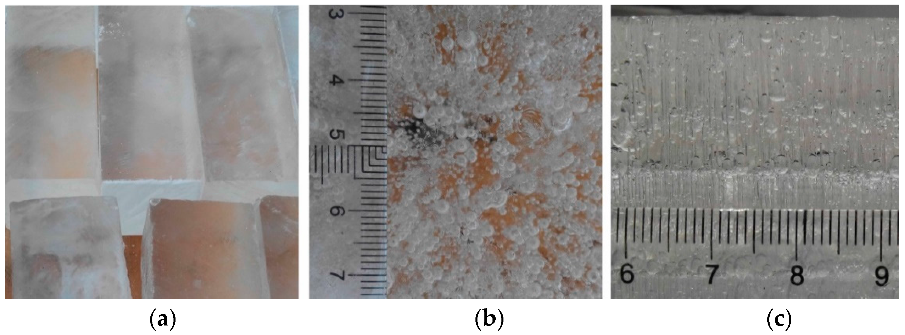
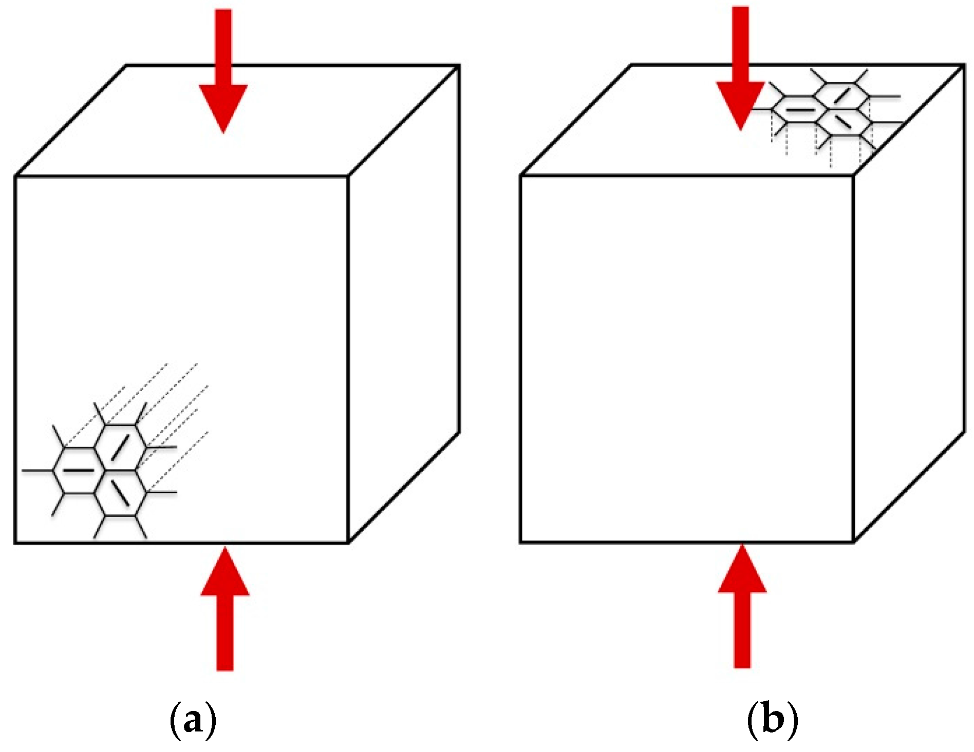
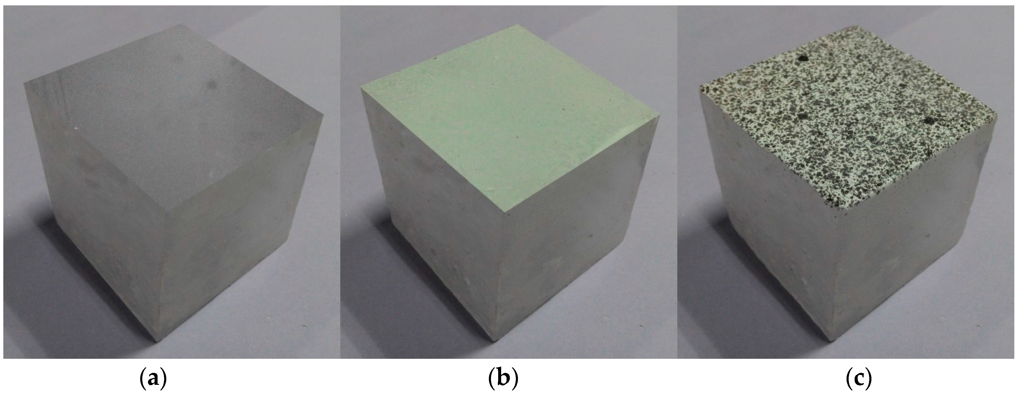
In the present experiments, ice specimens originate from natural lake ice. Experiments set up five loading rates, and two temperatures and two loading directions. The loading apparatus is a specially-developed high-speed testing machine which can supply a constant loading rate in the velocity range of 0.1–20.0 m·s⁻¹. A dynamic load monitoring system, made up of an upper load cell and a lower load cell, is developed and adopted to measure the dynamic load aiming at evaluating whether force at the upper-end is close to that of the bottom-end of a specimen during the course of high-speed loading. True dynamic deformation of ice specimens is obtained by use of the non-contacting digital speckle correlation method through constructing artificial speckle on surfaces of specimens in advance.

2.1. Ice Specimens

Natural ice, such as lake ice, river ice, and sea ice, is the most usually involved ice type in engineering. The majority of researchers preferred selecting artificial ice specimens rather than manufacturing specimens from natural ice in ice mechanical experiments, because it might take some risk to harvest ice blocks from the fields, in addition to significant amounts of time and energy being consumed. However, it is worth noting that some inherent characteristics of natural ice, such as impurities and air bubbles, cannot be constructed well in artificial ice. In order to allow for results to be more applicable to engineering applications, natural lake ice, which generally belongs to S2 type columnar ice [19], is chosen. Ice blocks are harvested in two periods, the stable freezing season and the early melting season, respectively. Ices harvested in different periods possess roughly the same grain size, which varies 2.0–7.0 mm in diameter. However, their air porosities are different. Ice collected during the stable freezing season, which we regard as “hard ice”, does not contain naked-eye visible air bubbles; while ice collected during the early melting season, which we regard as “soft ice”, contains a large number of naked-eye visible air bubbles that composed of dense, slender bubbles and a small amount of spherical bubbles, and the diameters of air bubbles vary 0.1–2.0 mm (as shown in Figure 1). Hard ice and soft ice possess average air porosities of 0.1% and 2.0%, respectively, based on apparent density measurements.

It takes three steps to manufacture an ice specimen from ice floes. Firstly, large-sized ice floes are harvested from the center site of an artificial lake. Then the ice floes are transported to a cold room, in which ice floes are processed into predetermined-sized ice specimens with a circular saw. Finally, using sandpaper or a belt sander, specimens’ surfaces are polished to ensure that the surfaces are smooth and the upper surfaces and lower surfaces must also be parallel, otherwise localized damage might occur under compression. Well-processed specimens were packed in labeled plastic bags, and then placed into a low constant temperature test chamber for storage. Before the test, ice specimens must reach the predetermined temperature and maintain at this temperature for not less than 48 h to ensure possessing a uniform temperature interior and exterior of the sample.

In previous experiments on the mechanical behavior of ice, generally −10 °C was selected as the test temperature [20]. For convenience of comparison with existing experimental results, −10 °C is selected as one of test temperatures and the other test temperature is −5 °C. In order to consider grain boundary effect, tens of grains should be contained in the minimum dimension of a specimen, so ice specimens cannot be too small. On the other hand, ice specimen cannot be too large in order to obtain equilibrium stress in the loading direction under high rate loading conditions. Giving a comprehensive consideration of the above-mentioned two factors, cubic ice specimen with an edge length of 5 cm is finally used in present experiments. Five loading rates, 0.1, 0.2, 0.5, 1.0, and 2.0 m·s⁻¹, are adopted. Half of the ice specimens are loaded along the length of columns and the others are loaded perpendicular to the length of columns (as shown in Figure 2). Under each test condition, there are at least three specimens, one non-speckle specimen, one pure white specimen, and one or more white-black speckle specimen (as shown in Figure 3). The non-speckle specimen is used for the observation of crack propagation and distribution within the ice sample; the pure-white specimen is used for observation of surface crack initiation and propagation; and the white-black speckle specimen is used for deformation measurement.

Tests are conducted at ambient temperature of −5 to −3 °C, accompanied by high-intensity lighting (which is necessary for high-speed camera to carry out high-speed recording and will be mentioned in the following paragraphs). If the ice specimen was exposed to ambient temperature and high-intensity lighting for a long time, ice might be warmed. While, as the time spent for a single test is usually very short (could be controlled in less than 30 s), the influences of ambient temperature and high-intensity lighting on ice could be negligible. In fact, this has been confirmed by the study of Render and Pan [21], who investigated high-speed impact characteristics of hailstones. Besides, in order to reduce the influence of lighting irradiation on platen temperature, we turn the strong light off and pause for some amount of time after 4 or 5 compression test cases.

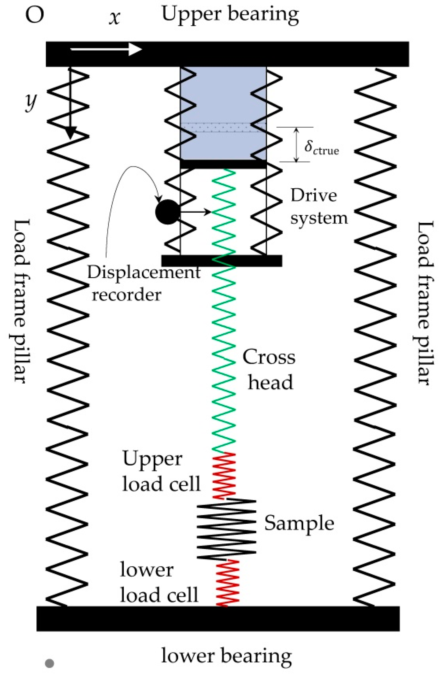
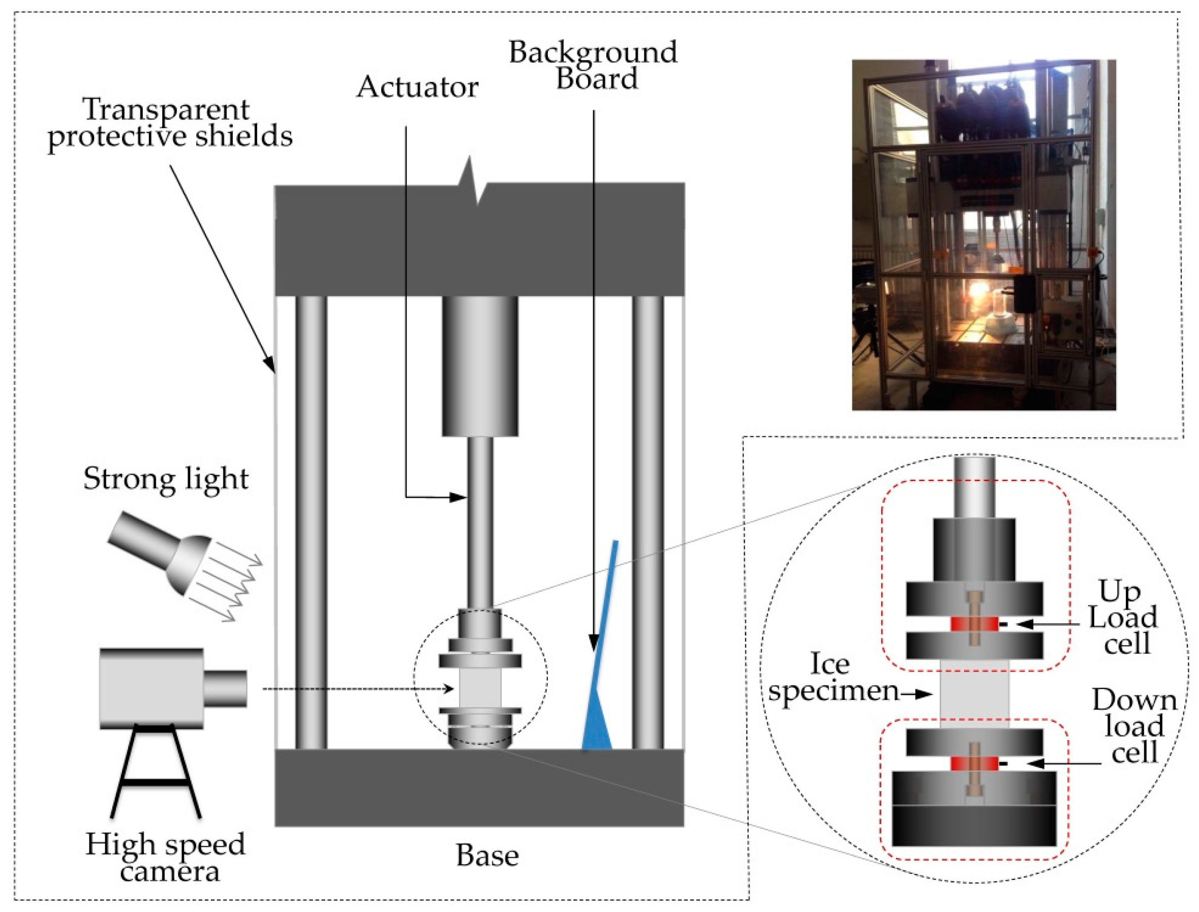
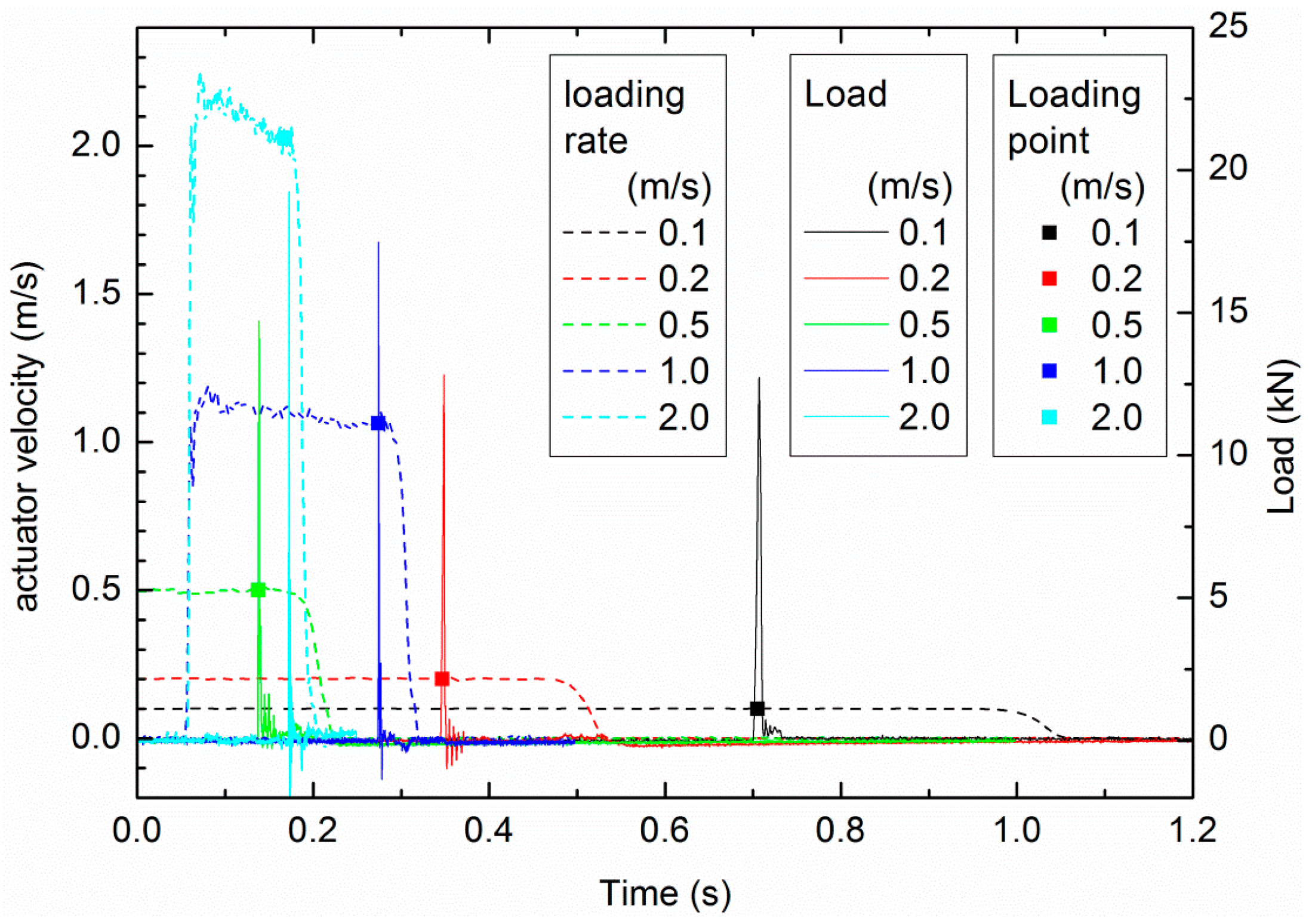
2.2. High-Speed Loading Machine with Two Load Cells for Dynamic Force Measurement

In the present experiments, a specially-developed high-speed testing machine is used as a dynamic loading apparatus, as shown in Figure 4. The most significant feature of this machine is that it supplies a constant loading rate in the speed range of 0.1–20.0 m·s⁻¹ with control precision of 0.1 m·s⁻¹. The nominal strain rate is in the range of 2–400 s⁻¹ if a 5-cm edge length cubic specimen is used. A universal testing machine can never supply such high strain rates. Moreover, the Instron impact machine can supply loading force up to 160 kN, so large-sized specimens can be used. The SHPB system can carry out experiments at very high strain rates, but the size of specimens which it used is limited, usually not larger than one centimeter in length, so effects of air bubbles and grain boundaries cannot be considered. Compared to the SHPB system, the Instron high-speed loading machine is able to load larger specimens, avoiding the drawbacks of losing some intrinsic characteristics of ice when using too small-sized specimens.

The Instron high-speed loading machine applies a servo control mechanism, hydraulic drive, and possesses a maximum actuator stroke of up to 600 mm. The actuator experiences acceleration, uniform speed, and slowdown three movement stages when loading. Actuator needs to travel a certain distance to accelerate to reach a pre-setting loading rate. The key to make ice specimen compressed at a pre-setting loading rate is to set the distance between platen and upper-surface of ice greater than that needed to reach the pre-setting loading rate, so the crosshead could contact with ice specimen at the pre-setting loading rate from the beginning of compression. The specimen is held for a very short time from beginning loading to finishing loading, so if the specimen is destroyed at uniform-speed movement stage, the specimen is regarded as being subject to uniform loading (as shown in Figure 5).

${\mathsf{\epsilon }}_{\mathrm{np}}$ denotes the nominal ultimate strain, ${\dot{\mathsf{\epsilon }}}_{\mathrm{n}}$ denotes the nominal strain rate, and ${\mathsf{\sigma }}_{\mathrm{c}}$ denotes the compressive strength; then, we have:

$${\mathsf{\epsilon }}_{\mathrm{np}}=\frac{{\mathsf{\delta }}_{\mathrm{p}}}{h}=\frac{v·\Delta t}{h}$$

(1)

$${\dot{\mathsf{\epsilon }}}_{\mathrm{n}}=\frac{{\mathsf{\epsilon }}_{\mathrm{np}}}{\Delta t}=\frac{v}{h}$$

(2)

$${\mathsf{\sigma }}_c=\frac{F_{\mathrm{p}}}{A}$$

(3)

where ${\mathsf{\delta }}_{\mathrm{p}}$ is the peak deformation of ice specimen, $h$ is the height of specimen, $v$ is the loading rate of the actuator, $\Delta t$ is the sustaining time from the start of loading to reaching peak load, $F_{\mathrm{p}}$ is the peak load, and $A$ is the cross-sectional area of specimen. In this article, the term nominal strain is used to refer to the ratio of displacement increment obtained from actuator to original height of sample, and the term nominal strain rate is used to refer to the ratio of nominal strain to corresponding time interval. Both terms are related to deformation recorded by testing machine.

In dynamic mechanical experiments, if the loading rate is too high, it is likely to form non-uniform stress due to the inertial effect. The loading rate should be lower than a threshold rate which is related to specimen length and material mechanical properties if we want to obtain the compressive strength at moderate rates. There are some theoretical formulas to consider the inertial effects [22,23], while ice mechanics are so complex that theoretical formulas may be invalid sometimes. Instead, a two-load-cell system is used for force measurement. The dynamic load cell has a natural frequency of 37 kHz and a force capacity of 50 kN. The upper load cell is connected to the actuator of the test machine, and the lower load cell is connected to the machine base. Loads at the upper-end and bottom-end of the specimen are measured at the same time, and profiles of the load versus time of the two load cells are compared.

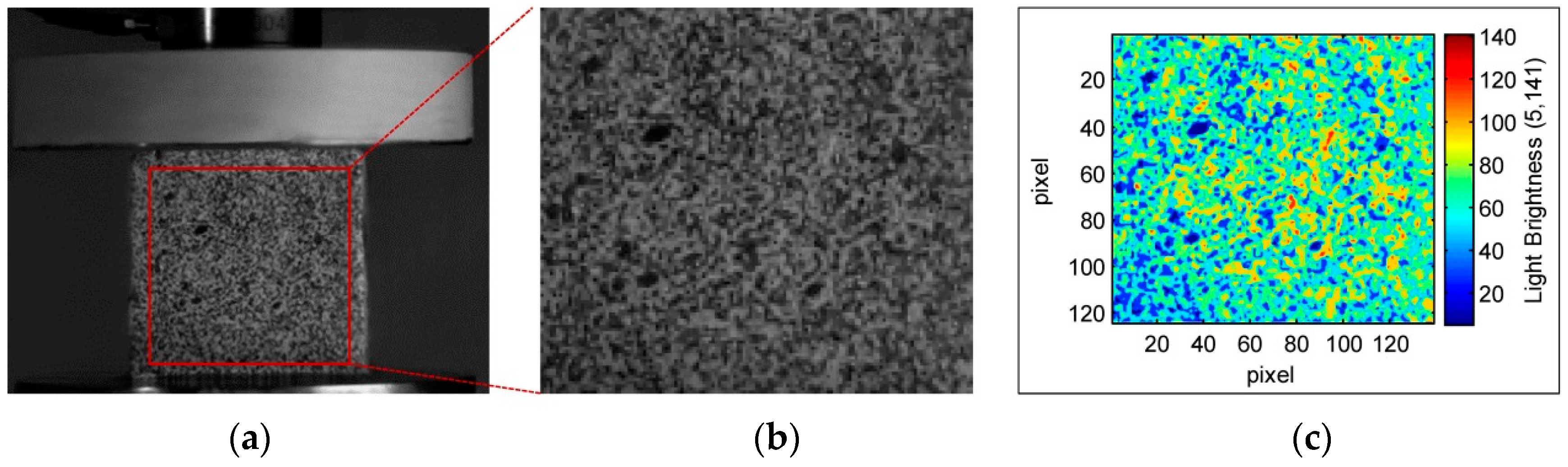
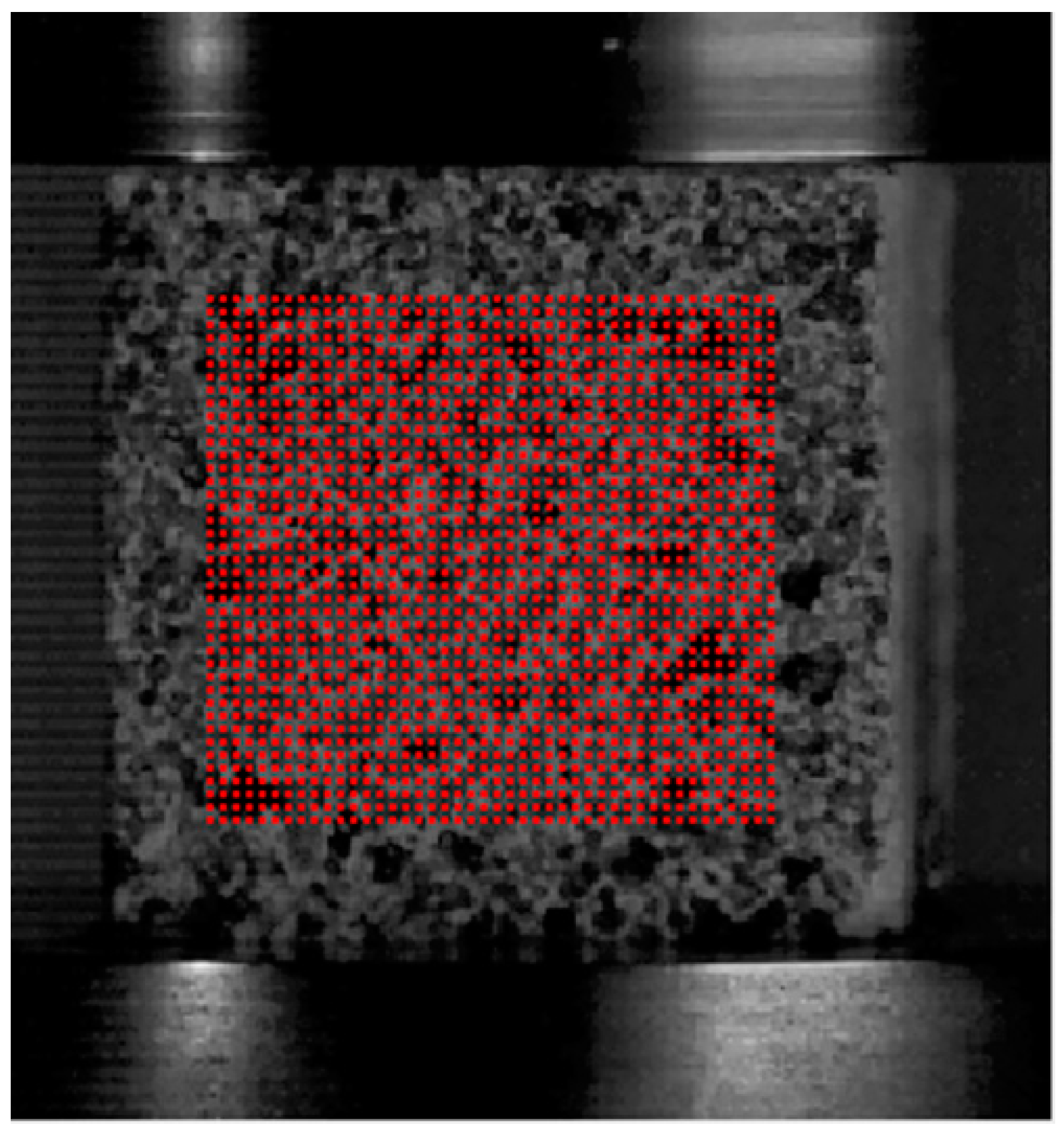
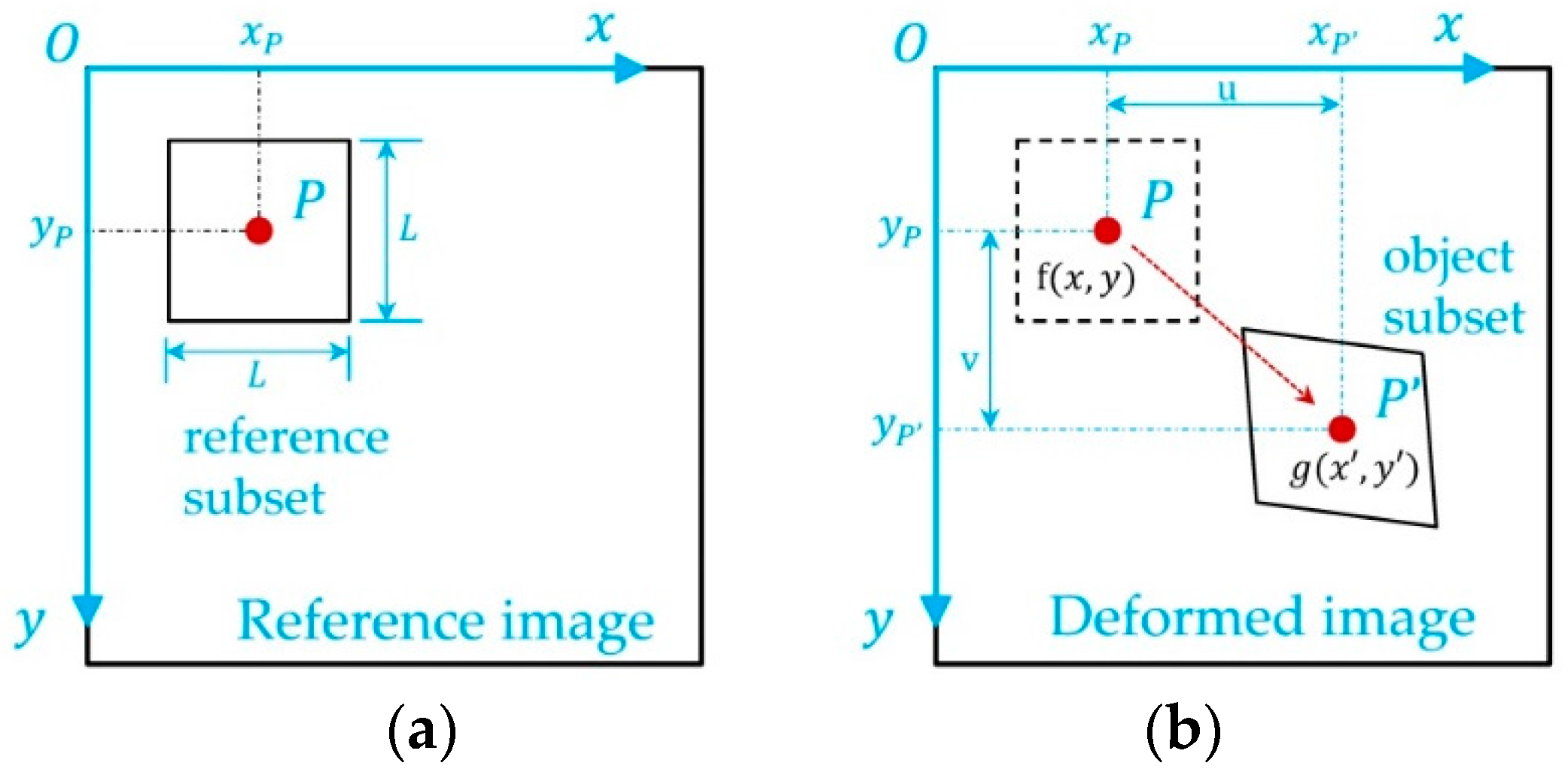
2.3. Digital Speckle Correlation Method for Deformation Measurement

In ice mechanics experiments, deformation of specimens is usually measured through measuring actuator displacement, conventional strain gauges, or an extensometer. Under creep and quasi-static conditions, these methods work well and were widely used; while these methods are not suitable for ice dynamic compression experiments due to restrictions resulting from material features of ice and their own limitations. Measuring actuator displacement is an indirect measurement, and nominal strain or strain-rate can be derived. The prerequisites are that the rigidity of the test machine is large enough and interfaces between the platens and specimen are perfect. The former prerequisite is easy to meet, but the latter prerequisite is not. It is difficult to use bond strain gauges on the surface of the ice specimen or freeze strain gauges in ice specimens; in addition, gauges may provide local reinforcement, which perturbs the stress field. The average strain can be obtained between two points by employing an extensometer, but the extensometer risks being damaged under dynamic loading. Furthermore, the inertia effect of the extensometer, itself, also affects the measurement results. In short, to measure the dynamic deformation of ice specimens requires applying a new feasible deformation measurement method.

The digital speckle correlation method is an optical deformation measurement method which is based on gray-scale analysis of speckle images [18]. The basic principle is calculating the pixel displacement by matching speckles between the un-deformed image and the deformed image, and then deriving information of strain and strain-rate. Compared with the traditional electrical measurement methods (such as the use of strain gauges, extensometer, etc.), the digital speckle correlation method breaks through the limitations of localized measurement, small deformation measurement, and contacting measurement, providing whole field information, large deformation measurement, and non-contacting measurement. Due to its non-contacting feature, deformation measurements of materials that cannot stick to strain gauges effectively can be achieved very well. Since it was put forward, the digital speckle correlation method has been developed into an important deformation measurement method in mechanical testing [24], such as biomechanical testing [25], mechanical testing of wood, rock, and composite materials [26,27], as well as crack propagation and other practical applications fields [28,29].

The digital speckle correlation method performs deformation measurement based on the correlation principle, as shown in Figure 6. The following steps should be taken to measure deformation by use of DSCM: First, select reference points in the reference image and determining an appropriate correlation subset zone with reference points located at the centers. Second, select appropriate correlation formulas for correlation computation to calculate pixel displacements of the reference points in the deformed images. There are many formulas that can be used for correlation computation [30]. A widely used cross-correlation formula is used:

$$C\left(\mathrm{u},\mathrm{v}\right)=\frac{{\displaystyle \sum {\displaystyle \sum \left[\left(f\left(x_i,y_j\right)-\overline{f}\left(x_i,y_j\right)\right)·\left(g\left(x_i^{\prime },y_j^{\prime }\right)-\overline{g}\left(x_i^{\prime },y_j^{\prime }\right)\right)\right]}}}{{\left[{\displaystyle \sum {\displaystyle \sum {\left(f\left(x_i,y_j\right)-\overline{f}\left(x_i,y_j\right)\right)}^2}}·{\displaystyle \sum {\displaystyle \sum {\left(g\left(x_i^{\prime },y_j^{\prime }\right)-\overline{g}\left(x_i^{\prime },y_j^{\prime }\right)\right)}^2}}\right]}^{1/2}}$$

(4)

where $f$ and $g$ are gray-scale functions of the reference image and deformed image, respectively. $\overline{f}$ and $\overline{g}$ are average values of $f$ and $g$, respectively. $x_i$ and $x_i^{\prime }$ are the coordinates of the $i$th pixel of the reference subset zone and the deformed subset zone in x direction, respectively. $y_j$ and $y_j^{\prime }$ are coordinates of the $j$th pixel of the un-deformed subset zone and the deformed subset zone in the y direction, respectively. $x_i^{\prime }=x_i+\mathrm{u}$ and $y_j^{\prime }=y_j+\mathrm{v}$. $\mathrm{u}$ and $\mathrm{v}$ are integer pixel displacement in the x direction and in the y direction, respectively. $C$ is the correlation coefficient and it depends on $\mathrm{u}$ and $\mathrm{v}$. Given a reference point P, the value (${\mathrm{u}}_0$ and ${\mathrm{v}}_0$) letting $C$ obtain a peak value is the integer pixel displacement of point P in the current deformed image.

After obtaining the integer pixel displacement, we also need to determine sub-pixel displacements of reference points in order to improve the deformation measurement accuracy. Recently, there exist many effective sub-pixel displacement calculation methods, such as the sub-pixel interpolation algorithm, correlation coefficient surface fitting method, coordinate rotation method, and the Newton–Raphson iterative method [31]. In this work, sub-pixel displacement calculation is carried out by use of a correlation coefficient surface fitting method which holds a strong anti-noise ability, high resolution, and high computational efficiency.

The digital speckle correlation method requires an image acquisition system consisting of high-intensity light sources and a high-speed camera (as shown in Figure 4). Two 300-W Raikage lights are arranged on both sides of the specimen. The highest imaging frequency of the high-speed camera is up to 100,000 frames per second (fps) and an imaging frequency of 50,000 fps is adopted in the present experiments. In order to obtain images with good quality, the centerline of the camera lens is perpendicular to the specimen speckle surface. The high-speed camera is triggered by the electrical signal of the loading control system.

The resolution of the digital speckle correlation method depends on various factors, such as image speckle quality and the correlation algorithm chosen [32]. Speckles, carrying the displacement information, are divided into natural speckles and artificial speckles. Different kinds of minerals contained in granite rock, which show different colors, consist of typical natural speckles. Materials without natural speckles, i.e., ice, should be pretreated to construct artificial speckles on their surface in order to use DSCM. Constructing artificial speckles include the following steps: (a) polishing the surface or zone that is to be observed; (b) spraying paint toward the interested specimen surface at a certain distance, ensuring that paint mists scatter to the surface to form speckles; and (c) when paint speckles on the surface are dry, repeating Step 2 with another color paint to form a multi-colored mixed speckle field. Generally, a combination of white paint and black paint is enough. In practice, it is found that speckle construction on the surface of ice specimen is much more difficult than that on the surface of rock and wood, because the former should be operated at subzero temperatures. Under such conditions the paint adhesion is worse than at room temperature. Through a trial-and-error method, we obtain some useful skills. Oil paint is more suitable than water-based paint for speckle field construction. First, we spray the whole surface with white paint, then spray paint of another color. Speckles on the surface of the specimen can be dried after 24 h; it is suggested that taking the specimen out and carrying out testing as soon as possible, otherwise small holes may emerge on the surface of the specimen which results in poor adhesion between paint and ice. The speckle size of a typical surface speckle field of ice specimens in the present experiments is in the range of 8–15 pixels, as shown in Figure 7.

3. Experimental Results

This section elaborates the experimental results of hard ice and soft ice under dynamic loading conditions.

3.1. Results of Dynamic Uniaxial Compression Tests on Hard Ice

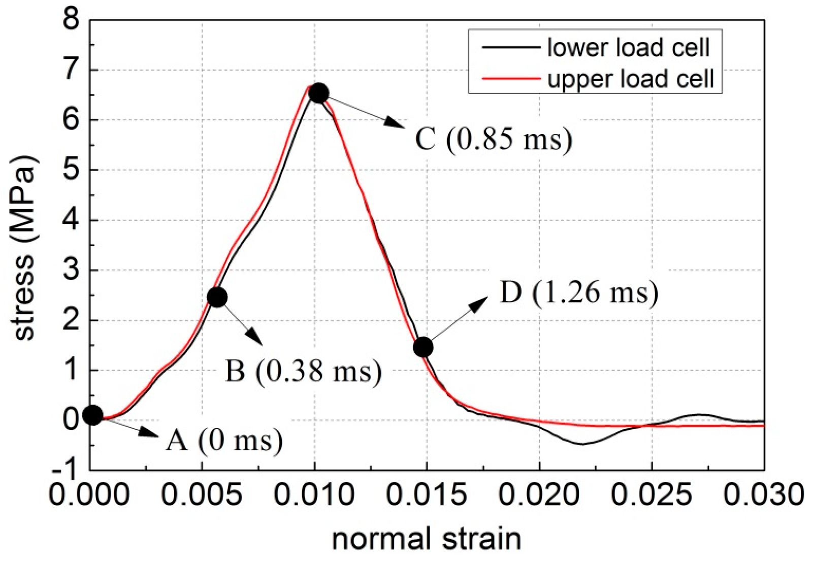
3.1.1. Uniaxial Compressive Strength of Hard Ice

Eighty 5-centimeter edge length cubic hard ice specimens that are created from ice blocks harvested during the stable freezing season are tested, and thirteen of them fail. Two testing temperatures, −5 °C and −10 °C, and two loading directions, along the length of the columns and perpendicular to the length of the columns, are chosen in the experiments. Under each temperature and loading direction, five loading rates, 0.1, 0.2, 0.5, 1.0, and 2.0 m·s⁻¹ are employed. The nominal strain-rate corresponding to these loading rates are 2.0, 4.0, 10.0, 20.0, and 40.0 s⁻¹, respectively.

Typical stress versus nominal strain-rate profiles of hard ice at different loading rates are shown in Figure 8. Peak stress derived from the upper load cell is greater than that derived from the lower load cell and the difference between them increases with an increasing loading rate. However, the differences are less than 10%, so ice specimens are deemed to achieve balanced forces in loading direction at these loading rates, and the inertial effect is negligible. The average values of the strength values derived from the upper and lower load cells are taken as the compressive strength of ice specimens.

The compressive strength results are shown in

Table 1. Uniaxial compressive strength results of hard ice with two temperatures, two loading directions and five loading rates.

Loading Rate (m·s−1)	Serial Number	Uniaxial Compressive Strength (MPa)
		−5 °C		−10 °C
		Horizontal Loading	Vertical Loading	Horizontal Loading	Vertical Loading
0.1	1	2.224	3.159	6.391	5.520
	2	5.187	3.271	5.462	7.143
	3	2.795	4.642	5.300	5.991
	4	-	3.702	-	-
0.2	1	3.410	5.049	7.306	7.112
	2	4.779	3.327	5.608	8.476
	3	3.370	2.974	8.380	7.459
	4	2.082	3.280	-	-
0.5	1	3.726	5.372	6.196	6.438
	2	3.277	3.970	6.627	6.869
	3	4.865	6.064	7.315	8.444
	4	5.288	8.294	-	-
1.0	1	2.944	3.826	7.117	6.472
	2	5.050	5.877	9.830	8.602
	3	4.007	7.391	6.001	6.126
	4	-	4.644	-	-
2.0	1	4.567	6.539	8.181	8.341
	2	7.413	9.553	7.020	12.949
	3	5.633	11.358	8.378	12.200
	4	-	6.242	-	-

- Denotes failed samples.

. In General, ice strength values at −10 °C are greater than that at −5 °C. In the nominal strain-rate range of 2–40 s⁻¹, at a testing temperature of −5 °C, uniaxial compressive strength values vary from 2.0 to 10.0 MPa with an average strength value of 6.0 MPa. While, at a testing temperature of −10 °C, uniaxial compressive strength values vary from 5.0 to 12.0 MPa with an average strength value of 8.5 MPa. Standard deviations of result data are in the range of 1.0–2.0 MPa, varying with nominal strain-rate. Though there is a great scatter in data, the compressive strength shows an increasing trend with increasing loading rate. Through comparing compressive strength values of hard ice in different loading directions, it could be found that strength along the length of the columns is slightly stronger than that perpendicular to the length of the columns.

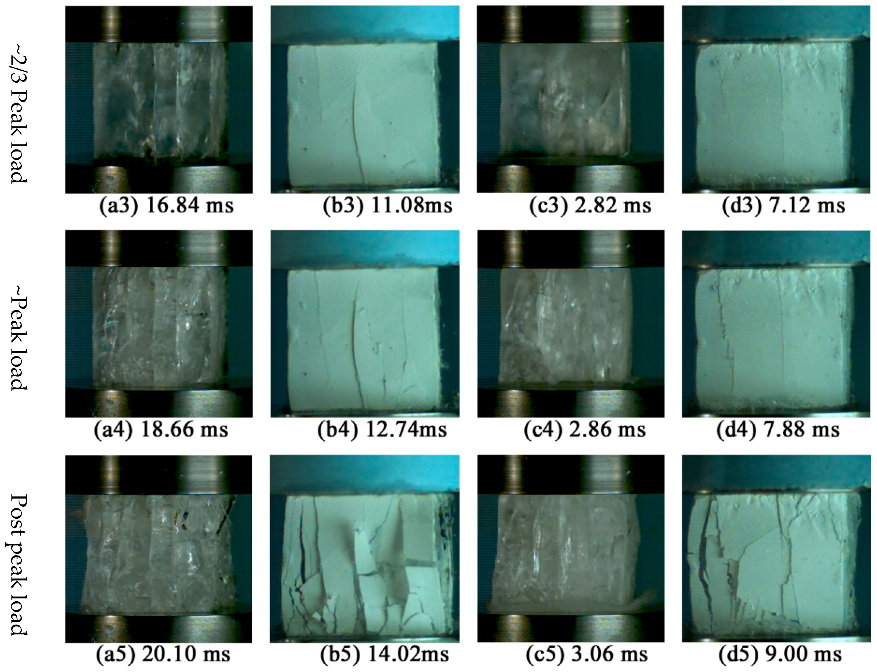
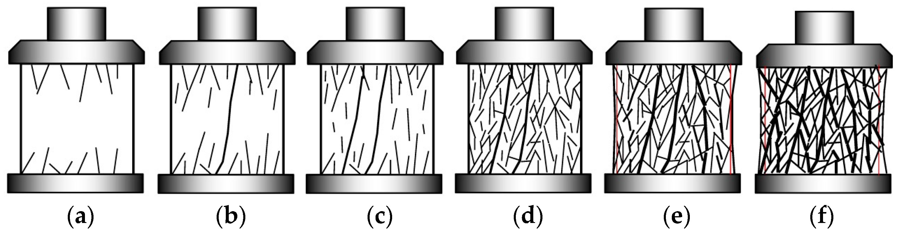
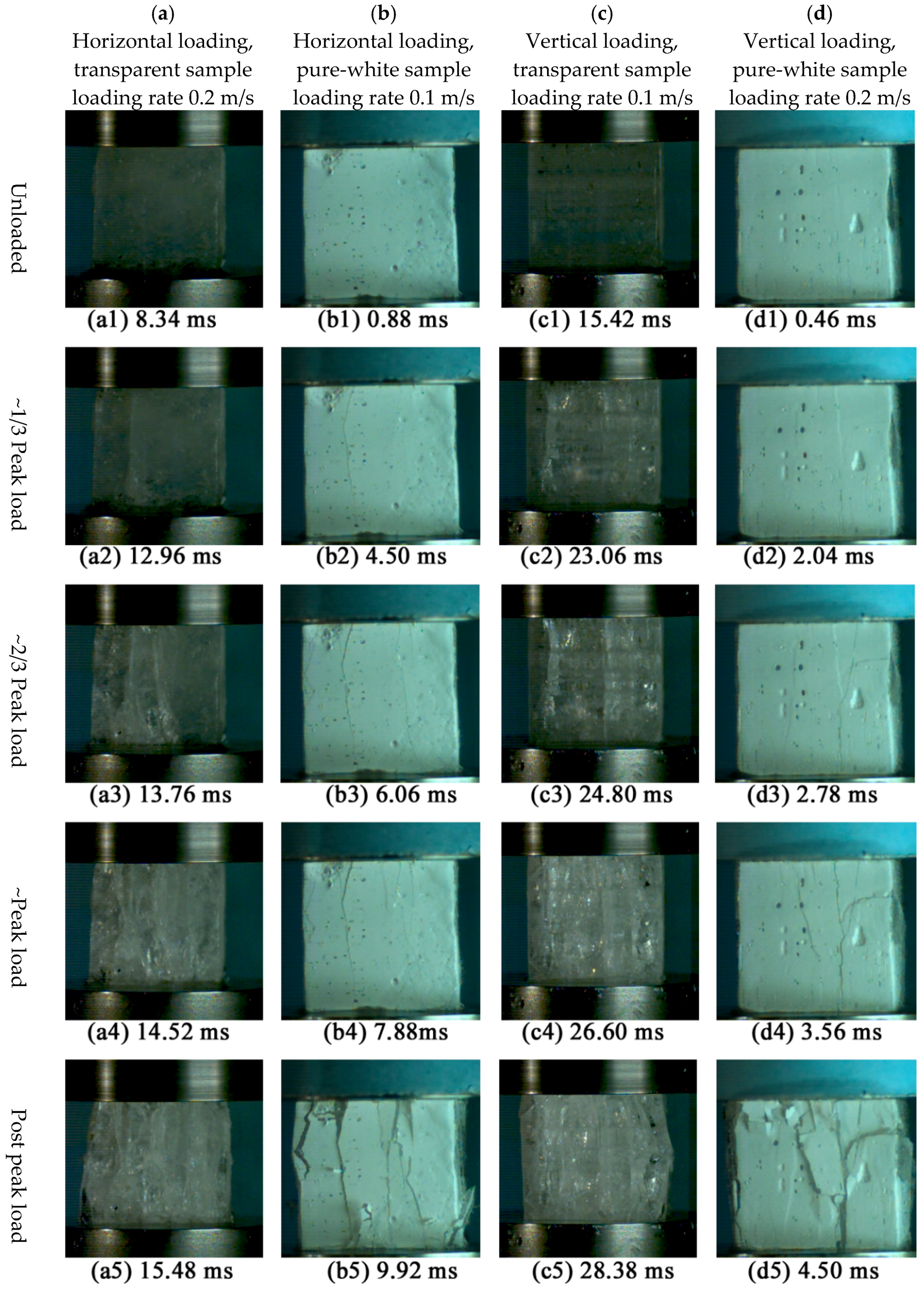
3.1.2. Fracture Mode of Hard Ice

A high-speed camera is employed to capture the failure processes of ice samples. Fracture processes of hard ice under uniaxial compression tests at moderate strain rates are shown in Figure 9. Images corresponding to five load levels—unloaded, 1/3 peak load, 2/3 peak load, peak load, and post peak load—are selected to illustrate the fracture processes. In the employed strain-rate range, fracture processes are not sensitive to strain-rate, and no clear distinguishing of fracture processes exists between horizontal loading and vertical loading. Ice samples fail in a mode which possesses features of splitting failure mode and features of crushing failure mode at the same time. Firstly, a few initial cracks emerge at the top end and bottom end of the sample. Then these initial cracks quickly propagate vertically or approximately vertically, leading to formation of full-height vertical cracks. Meanwhile, the crack density is low. As the sample is compressed further, the crack density within the sample increases and then several full-height vertical cracks form quickly. As more and more cracks emerge, a majority of intersections and link-ups of cracks form and the widths of full-height vertical cracks increase. At this moment, peak load is approximately reached. Horizontal expansion is observed with further compression, and then increase of the cracks’ width, resulting from slipping among cracks, is the main course, accompanied with slow increase of crack density. The sample fails, in appearance, in the splitting failure mode and is finally separated into lots of small fragments. It seems that full-height vertical crack formation is a little easier when the sample is loaded in the horizontal direction than when it is loaded in the vertical direction. When we compare the failure processes shown in Figure 9a and that shown in Figure 9c, we find the former shows the above-mentioned characteristics more obviously. Nevertheless, there exist no significant differences in fracture processes between horizontal loading and vertical loading, according to our careful observations on the time-sequenced failure images of tests in different loading directions.

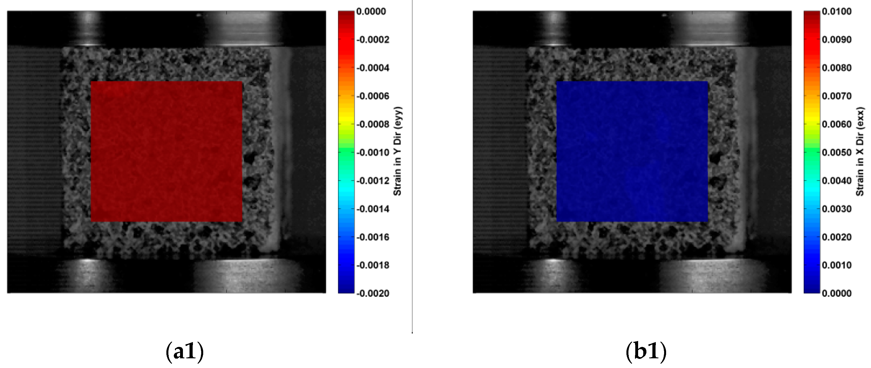
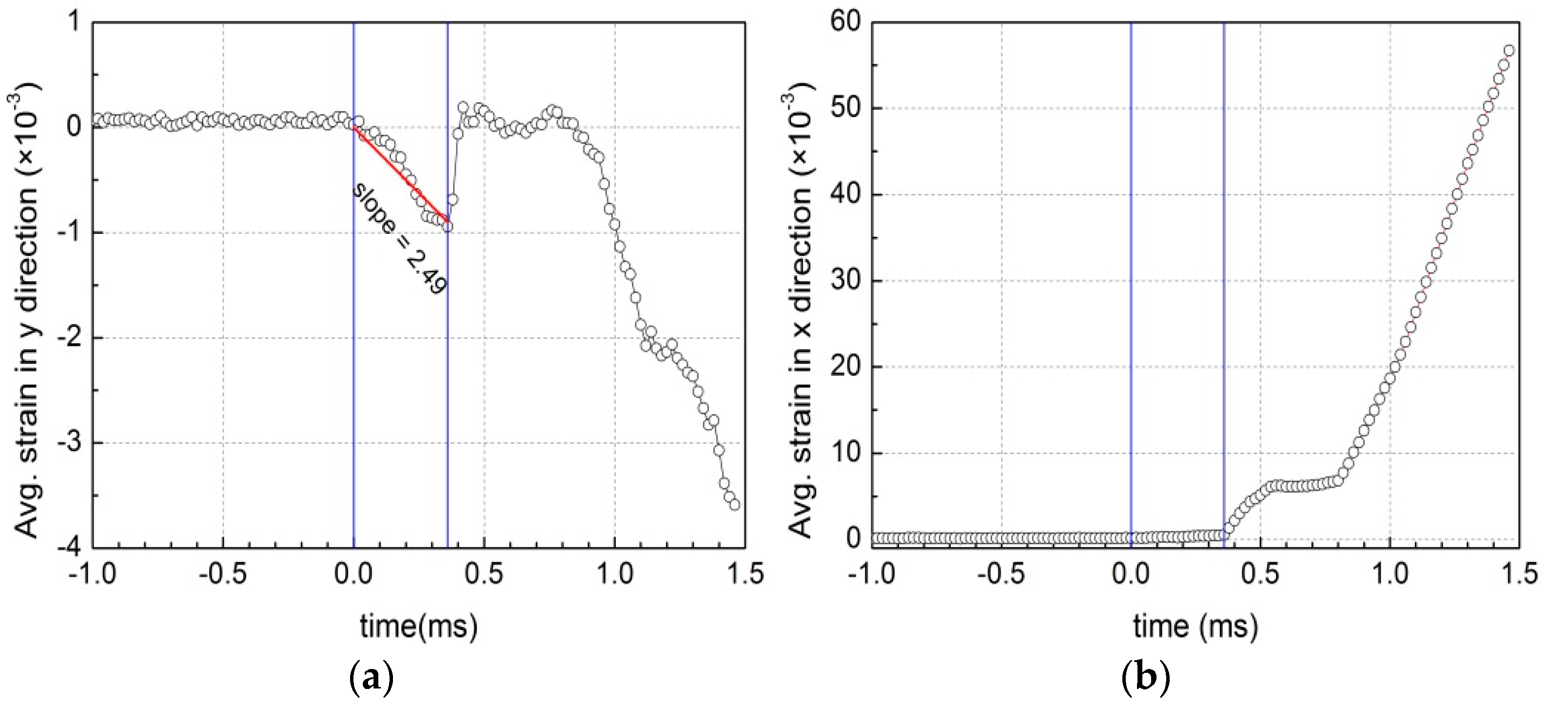
3.1.3. Dynamic Deformation Measurement by DSCM

It can be seen in Figure 8 that the nominal ultimate strain corresponding to peak stress varies from 0.5 to 1.2% and these values are obviously greater than the true ultimate strain values of ice under uniaxial compression. In order to measure the true deformation of an ice specimen, the non-contacting digital speckle correlation method is used for deformation measurement. In the following paragraph, the sample named “HH05mps2” is taken as an example to elaborate the deformation measurement results by means of DSCM. The label “HH05mps2” means the hard ice sample which is loaded with a 0.5 m·s⁻¹ loading rate along the horizontal direction, and its serial number is 2.

The stress versus nominal strain-rate profile of sample HH05mps2 is shown in Figure 10. Labels A, B, C, and D correspond to four time points of loading process. A is the moment of starting loading and this moment is regarded as the initial time point, so A corresponds to time point 0 ms. B is the moment when a certain load is reached, but the load can continue increasing. It corresponds to time point 0.38 ms. C is the moment when peak load is reached, and corresponds to time point 0.85 ms. D is the moment when the ice specimen is nearly total fail, corresponding to time point 1.26 ms. A reference point set of 41 points in vertical direction and 44 points in horizontal direction is built, and the spacing between the adjacent.

Reference points are three pixels (as shown in Figure 11). The size of the subset zone of each reference point is 21 by 21 pixels, and reference point locates at center.

The pixel displacement of each reference point is calculated firstly, and then the strain. In order to be intuitive, results are showed in terms of strain, instead of pixel displacement. Local strain results of the speckle surface at A, B, C, D four different moments are shown in Figure 12, figures in the left column correspond to the strain in the y-direction and right correspond to strain in x-direction. With regard to the strain in the y-direction, it should be compression strain all the time and increase with time; while, it is not exactly the same as what is expected. At starting moment A, strain in the y-direction is uniform (as shown in Figure 12(a1)); strain values are less than 0.06‰, as ice specimen is not loaded. At moment B, load increases to approximately half of the peak load; strain in the y-direction also increases obviously. Strain values are in the range of 0.6‰ to 1.0‰, with an average value of 0.8‰ (as shown in Figure 12(a2)). It is approximately uniform, though not as uniform as that at moment A. Actually ice specimen experiences almost uniform deformation in the y-direction. However, a small difference in y-direction relative displacements (i.e., displacement of interest reference point with respect to that of its furthest front reference point) may lead to an obvious difference in strains. As the strain field is derived from displacement field, numerical errors exist during derivation and the difference may be amplified. At moment C, the peak load is reached; while strain in the y-direction does not increase when compared with that at moment B. On the contrary, strain values in most of surface regions reduce to less than 0.1‰, local strain even is in tension form in some regions. There are also regions in which strain values increase up to ~1.4‰ (as shown in Figure 12(a3)). The strain field is considerable uneven. How does this happen? In fact, this can be associated with damage occurring in ice sample. When ice sample is divided into several parts by cracks, integrity of the speckle surface is destroyed. Some parts may still closely connect to a main bearing ice column, while some parts may not. If the part that contains certain speckle surface region connects to a main bearing ice column, this speckle surface region may deform with the bearing ice column together. On the other hand, if that part does not connect to a main bearing ice column, this speckle surface region may not deform further, or even deform reversely when the surrounding constraint is not sufficient. That is to say, at a moment ago, a reference point moves downward, while at a moment in the future it may move upward owning to separation from the main bearing column of ice sample. This scenario is similar to that a spring restores to its original length after the applied force is removed. In a word, when sample has not been damaged or have been just slightly damaged, the local strains derived from the pixel placements of the speckle surface can represent deformation of the exterior and interior of sample; While, when sample has been damaged by cracks, the local strains can still represent deformation of sample surface, but they might not represent deformation of the interior of sample again. Thus, at moment C, regions with small strain values should have separated from the main bearing column. While regions with large compression strain values should still connect to the main bearing column, so the reference points attached on these regions can continue shortening the distances between each other. At this moment, the local strains of the speckle surface cannot represent the deformation of the interior of sample again, and perhaps cause an illusion that the sample has not been in compression state again, but the sample is actually under compression state. At moment D, load decreases to a low level, the whole speckle surface is in compression state according to the strain contour shown in Figure 12(a4). The strain field is severally uneven. The upper section is compressed severally, with maximum strain value up to 5.0‰, while the lower section is compressed slightly, with minimum strain value even close to zero. The non-uniform appearance in strain field feature can also be explained in the way that we have done at moment C. With regard to strains in the x-direction at four different moments, they are all tension strain. At moments A and B, strain values are both smaller than 0.4‰ (as shown in Figure 12(b1,b2)), indicating only a slight expansion exists in the horizontal direction. When ice is compressed further, obvious expansion is found. At moment C, an obvious region in which strain values in the x-direction are higher than 10‰ appears (as shown in Figure 12(b3)), indicating a vertical crack has formed within this region and this is consistent with crack observation by naked-eye. At moment D, the strain values in most of the surface regions are greater than 10‰, and a value of 97‰ is obtained in the vertical middle region (as shown in Figure 12(b4)). This appearance indicates ice sample has expanded considerably in the horizontal direction, consistent with the fact that at this moment ice has been severally destroyed by cracks (as shown in Figure 9(a5,c5)).

Strain field derived from pixel displacement field can be used to estimate whether the sample deformation in the compression test is uniform. According to strain contours shown in Figure 12, not all strain fields obtained before the peak load moment (moment C) are uniform; so it is not a feasible way to calculate the true strain-rate directly by these strain fields, for the strain field cannot reflect the true deformation of ice sample again when lots of cracks has formed in ice sample. Instead, we fit the pixel displacements of all reference points with respect to their coordinates by means of linear least squares approach, thus the average true strain can be obtained, and then the average true strain-rate. The average true strains in the y-direction and x-direction are shown in Figure 13. With regard to the average true strain in the y-direction, strain values before loading starts (moment A) are almost all zero. After loading starts it gradually increases, accompanied with slight fluctuation, until to time point 0.38 ms (moment B). At this moment, the average true strain is 0.8‰, equal to the mean value of current local strain field (as shown in Figure 12(a2)). Thereafter, a sharp jump occurs. The average true strain reduces to a value near zero. Just after time point 0.38 ms, a large crack may form suddenly in ice sample, resulting in lots of speckle surface regions separated from the main ice body partially or totally and unloaded. According to analysis in the previous paragraph, the reference points within these regions will not continue shortening the distance between each other; instead, they restore to their original relative positions. Thus, the average true strain changes suddenly and drops down to a value near zero. As compression continues, the unloaded speckle surface regions may become loaded again, and then the average true strain increases again. The profile of average true strain versus time after time point 0.7 ms shows such scenario (as shown in Figure 13a). With regard to the average true strain in the x-direction, it is derived from pixel displacement in the x-direction. Before obvious cracks emerge, the average true strain increases slowly; once many obvious cracks emerge, it increases dramatically (as shown in Figure 13b). This is consistent with the result shown in Figure 9. Only the profile section, in whose corresponding time period detachment in ice sample has not yet occurred, are valid to deriving the average true strain-rate in the y-direction (as shown in Figure 13a, the profile section between the two blue lines is valid). The average true strain-rate of sample HH05mps2 in the y-direction is 2.49 m·s⁻¹, while the nominal strain-rate is 10.0 m·s⁻¹; the former is only approximately a quarter of the latter. In-negligible deformation of loading machine itself and imperfect interfaces between ice sample and platens account for this (a detailed analysis is conducted in the Appendix A). Multiplying the average true strain-rate by the sustaining time from the initial loading moment to the moment of achieving peak load, the true ultimate strain could also be obtained. Results of average true strain-rate and true ultimate strain under different loading rates and at different temperatures are shown in

Table 2. Ultimate strain and strain-rate results of hard ice derived from actuator displacement and DSCM. HH denotes the hard ice sample loaded in the horizontal direction; HV denotes the hard ice sample loaded in the vertical direction.

Temperature (°C)	Sample Name	Nominal Strain-Rate (s−1)	Sustaining Time (ms)	Average True Strain-Rate (s−1)	Nominal Ultimate Strain (%)	True Ultimate Strain (‰)
−5	HV01mps3	2	4.80	0.56	0.96	2.69
	HV02mps2	4	2.30	1.20	0.92	2.76
	HV05mps3	10	1.05	2.20	1.05	2.31
	HV1mps3	20	0.24	5.29	0.48	1.27
	HV2mps2	40	0.11	10.26	0.44	1.13
	HH01mps2	2	5.20	0.47	1.04	2.44
	HH02mps2	4	2.45	1.02	0.98	2.50
	HH05mps2	10	1.08	2.10	1.08	2.27
	HH1mps2	20	0.45	4.65	0.90	2.09
	HH2mps2	40	0.14	9.14	0.56	1.28
−10	HV01mps3	2	4.84	0.43	0.97	2.08
	HV02mps2	4	2.36	0.97	0.94	2.29
	HV05mps2	10	1.18	2.11	1.18	2.49
	HV1mps3	20	0.20	4.93	0.40	0.99
	HV2mps3	40	0.11	9.01	0.44	0.99
	HH01mps2	2	5.20	0.49	1.04	2.55
	HH02mps3	4	2.00	1.20	0.80	2.40
	HH05mps2	10	0.85	2.49	0.85	2.12
	HH1mps2	20	0.25	5.38	0.50	1.35
	HH2mps2	40	0.13	9.65	0.52	1.25

.

According to Table 2, obviously, there is a significant difference between nominal ultimate strain and true ultimate strain, as well as nominal strain-rate and average true strain-rate, and the formers are greater than the latters. As the loading rate becomes great enough, the ice specimen is more likely to fail in a crushing mode and achieve peak load at a relatively small nominal ultimate strain, as shown in Figure 8 and Table 2. The trend of failure in splitting mode is not as obvious as that at relative lower loading rates.

3.2. Results of Dynamic Uniaxial Compression Tests on Soft Ice

3.2.1. Uniaxial Compressive Strength of Soft Ice

Testing conditions of soft ice, which is collected during the early melting season, are the same as that of hard ice. The significant difference between soft ice and hard ice is the air porosity: the former contains obvious air bubbles and has a higher air porosity than the latter. Typical stress versus nominal strain profiles of soft ice specimens are shown in Figure 14. Under the employed loading rates, stress profiles increase uniformly before reaching the peaks and they do not drop rapidly after the peaks. Similar to profiles of hard ice specimens, peak stress derived from the upper load cell is greater than that derived from the lower load cell and the difference between them increases with increasing loading rate. However, the differences are less than 10%, so ice specimens are deemed to achieve balanced force in the loading direction at these loading rates, and the inertial effect is negligible.

The compressive strength results of soft ice are shown in

Table 3. Uniaxial compressive strength results of soft ice with two temperatures, two loading directions, and five loading rates.

Loading Rate (m·s−1)	Serial Number	Compressive Strength (MPa)
		−5 °C		−10 °C
		Horizontal Loading	Vertical Loading	Horizontal Loading	Vertical Loading
0.1	1	2.912	4.859	2.989	4.862
	2	2.548	3.001	4.130	6.423
	3	1.664	3.908	4.618	3.160
	4	1.170	4.119	3.426	7.300
	5	2.543	-	4.011	-
	6	3.228	-	-	-
	7	1.970	-	-	-
0.2	1	1.809	4.743	3.680	7.171
	2	2.012	3.107	4.200	8.402
	3	3.966	5.722	4.235	4.893
	4	2.646	-	4.499	-
	5	1.939	-	-	-
0.5	1	1.541	2.975	4.512	5.814
	2	1.905	5.782	4.911	4.823
	3	1.543	4.268	3.600	6.466
	4	2.863	-	-	-
1.0	1	2.310	3.565	4.236	6.135
	2	3.445	4.211	3.936	7.586
	3	3.100	5.522	5.130	6.550
	4	1.735	-	-	-
2.0	1	3.183	5.651	6.226	6.982
	2	4.157	4.790	4.866	8.861
	3	2.491	7.049	5.825	11.349
	4	1.966	-	-	-

- Denotes failed samples.

. In the strain-rate range of 2.0–40.0 s⁻¹, uniaxial compressive strength values vary from 1.2 to 7.0 MPa with an average strength value of 4.0 MPa at −5 °C. Uniaxial compressive strength values vary from 2.0 to 10.0 MPa with an average strength value of 6.0 MPa at −10 °C. Compared with hard ice, the strength of soft ice is weaker under the same testing condition, however, the characteristics showed by soft ice and that of hard ice are similar. Compressive strength increases with increasing loading rate and the strength along the length of the columns is slightly greater than that perpendicular to the length of the columns. Ice shows greater compressive strength at lower temperature.

3.2.2. Fracture Mode of Soft Ice

Fracture processes of soft ice under uniaxial compression tests at moderate strain rates are shown in Figure 15. Failure images at five load levels are selected to illustrate the failure processes. It shows that the failure process of soft ice is similar to that of hard ice at moderate strain rates. Cracks are firstly observed at the ends of sample, and then obvious full-height vertical cracks are observed. When load reaches the peak value, the crack density within the sample is high and the sample becomes milky white. Finally, the sample fails in the splitting mode in appearance, accompanied with many fragments. It seems that air bubbles existing in soft ice sample do not have an obvious effect on the fracture mode.

3.2.3. Dynamic Deformation Measurement by DSCM

Table 4. Ultimate strain and strain-rate results of soft ice derived from actuator displacement and DSCM. SH denotes soft ice sample loaded in the horizontal direction, SV denotes soft ice sample loaded in the vertical direction.

Temperature (°C)	Sample Name	Nominal Strain-Rate (s−1)	Sustaining Time (ms)	Average True Strain-Rate (s−1)	Nominal Ultimate Strain (%)	True Ultimate Strain (‰)
−5	SH01mps4	2	4.51	0.44	0.90	1.98
	SH02mps3	4	2.36	1.09	0.94	2.57
	SH05mps3	10	0.84	2.79	0.84	2.34
	SH1mps2	20	0.23	5.78	0.46	1.33
	SH2mps3	40	0.16	9.16	0.64	1.47
	SV01mps3	2	5.50	0.56	1.10	3.08
	SV02mps3	4	2.35	0.89	0.94	2.09
	SV05mps2	10	1.21	2.73	1.21	3.30
	SV1mps2	20	0.20	4.31	0.40	0.86
	SV2mps3	40	0.11	9.35	0.44	1.03
−10	SH01mps5	2	6.19	0.41	1.24	2.54
	SH02mps3	4	2.80	0.88	1.12	2.46
	SH05mps2	10	0.97	2.27	0.97	2.20
	SH1mps3	20	0.41	5.46	0.82	2.24
	SH2mps2	40	0.12	9.15	0.48	1.10
	SV01mps2	2	6.03	0.48	1.21	2.89
	SV02mps2	4	2.24	1.14	0.90	2.55
	SV05mps3	10	1.26	2.01	1.26	2.53
	SV1mps3	20	0.28	5.98	0.56	1.67
	SV2mps3	40	0.15	9.53	0.60	1.43

shows ultimate strain and strain-rate results of soft ice under different loading rates. Nominal ultimate strain values are in the range of 0.5–1.3%, while true ultimate strain values are much lower, in the range of 1.0–2.6‰. Similar to results of hard ice, there is a great difference between nominal strain-rate and true strain rate under dynamic loading condition. The true strain-rate is approximately 1/4 of the nominal strain-rate.

4. Summary of Results and Discussion

4.1. Dynamic Deformation of Ice Samples at Moderate Rates

In the present experiments, a two-dimensional digital speckle correlation method is employed to measure deformation of ice specimens under dynamic loading conditions. This is the first time to apply DSCM for ice mechanical properties investigation and results show that it is suitable to measure dynamic deformation of ice specimens. The key to using the digital image speckle method is constructing a high-quality speckle field on surfaces of ice specimen. An imaging rate of 50,000 fps is enough to capture failure process of ice when the loading rate is not greater than 2.0 m·s⁻¹ and sample is 5 cm high. A higher imaging rate may achieve better results, as ice is an extremely brittle material and ice sample may fails in several milliseconds.

Both true strain-rate and nominal strain-rate are calculated; the former is obtained by DSCM and the latter is derived from actuator displacement. Results of true strain-rate and nominal strain-rate under different loading rates and at different temperatures are shown in Figure 16a. The true strain-rate is approximately 1/4 of the nominal strain-rate. Results of nominal ultimate strain and true ultimate strain are shown in Figure 16b. Nominal ultimate strain in these experiments varies from 0.4 to 1.3%, while true ultimate strain varies from 0.9‰ to 3.2‰. Nominal ultimate strain is greater than the true ultimate strain, and the latter is approximately 1/4 of the former. That is to say, the true strain-rate is obviously distinguished from nominal strain-rate. The large difference may result from imperfect specimens and the loading system. Load-bearing surfaces could not be perfectly smooth though fine polish is applied to ice specimen surfaces. Tiny concavities or convexities in surface may increase the measured deformation, resulting in greater nominal ultimate strain. Slightly incomplete parallelism between the top and bottom load bearing faces could result in a slight rotation of the specimen under compression, which can also result in an increase of nominal ultimate strain. Stiffness of the loading system also has an important influence on sample deformation (a detailed analysis is shown in Appendix A). Taking only the deformation of the actuator into consideration, deformation of machine may lead to true deformation significantly less than the machine measured deformation. For this reason, it is necessary to measure the true deformation of ice specimens by DSCM in dynamical compression experiments. The nominal strain-rate chosen in the present study is in the range of 2–40 s⁻¹, while the true strain rate is in the range of 0.4–10.0 s⁻¹.

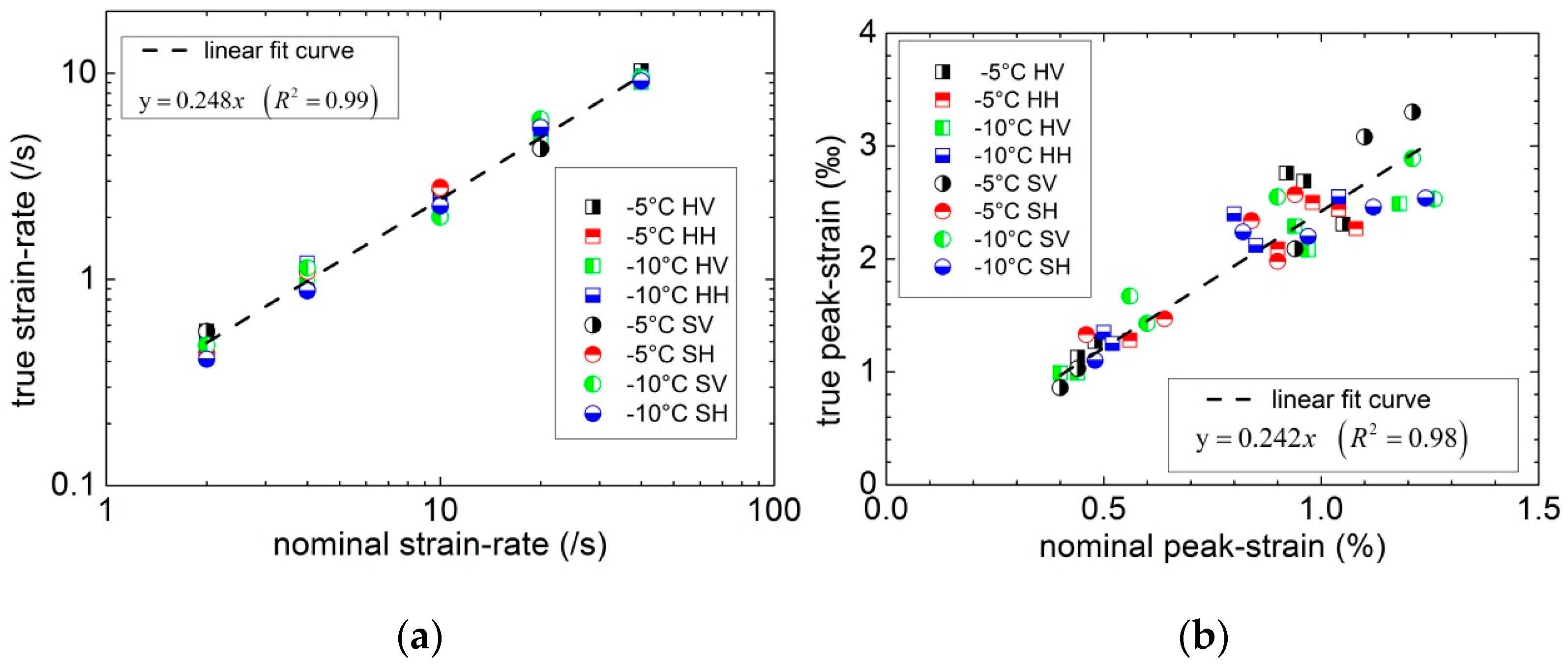
4.2. Relationship between Compressive Strength and Strain-Rate, Air Porosity, Loading Direction as Well as Temperature in Moderate Strain-Rate Range

By means of DSCM, the true strain-rate can be obtained. Results of uniaxial compressive strength versus true strain-rate are shown in Figure 17. The uniaxial compressive strength results show huge scatter and it is more serious in soft ice. As many previous studies have reported, huge scatter may be due to internal structure differences between ice specimens and imperfect interfaces between platen and ice surface. In the present work, ice grain size varies 2.0–7.0 mm in diameter based on measurement results of some samples. As not all of the grain sizes of specimens are measured, we cannot relate the difference in strength to grain size quantitatively. However, it has been well confirmed that ice with smaller grain size trends to obtain a greater strength value [16]. The grain size difference in experimental specimens could be a significant reason for the huge scatter. In soft ice, besides the difference in grain sizes, the difference in air bubbles contained in different ice specimens is also a factor in making ice strength scattered. Therefore, strength data of soft ice show greater scatter than that of hard ice. In addition, it is difficult to ensure perfect interface between platen and ice surface though ice specimens are finely machined. Loading direction seems to have little effect on strength scatter. Though a significant scatter exists in strength data, it does not evidently affect us analyzing the relationships between compressive strength and strain-rate, air porosity, loading direction as well as temperature.

Two kinds of ice with different air porosities are used in experiments: hard ice with an average air porosity of 0.1% and soft ice with an average air porosity of 2.0%. In the strain-rate range of 0.4–10.0 s⁻¹, at −5 °C, for hard ice, the average horizontal and vertical compressive strength are 4.0 MPa and 5.0 MPa, respectively. For soft ice, they are 2.5 MPa and 4.5 MPa, respectively. At −10 °C, for hard ice, they are 7.0 MPa and 8.0 MPa, respectively, while, for soft ice, they are 4.5 MPa and 6.5 MPa, respectively. The compressive strength of hard ice at −10 °C is 1.75 times that at −5 °C when loading horizontally, and 1.60 times when loading vertically. For soft ice, strength at −10 °C is 1.80 times that at −5 °C when loading horizontally, and 1.44 times when loading vertically. Even though the ices have different air porosities, both are affected by temperature significantly, no matter whether loading horizontally or vertically. Dutta et al. [8] also investigated ice compressive strength at −10 °C and −40 °C at about 10 s⁻¹ strain-rate. Study of Dutta et al. showed that the average strength of ice was 4.70 MPa at −10 °C and 5.81 MPa at −40 °C (excluding strength data of bonded-end samples). The latter is 1.2 times the former. By comparison with the result of Dutta et al., ice compressive strength seems to be more sensitive on temperature in the higher temperature range. Actually, under quasi-static conditions, similar observation is also found [33,34]. However, quantitative analysis on the rate of change of the compressive strength at moderate strain rates with respect to temperature in different temperature ranges needs further investigation.

When loaded horizontally, the average strength of hard ice is 1.6 times that of soft ice at −5 °C, and 1.7 times at −10 °C. While when loaded vertically, the average strength of hard ice is only 1.1 times that of soft ice at −5 °C, and 1.2 times at −10 °C. Air porosity weakens ice strength and has a greater influence on the horizontal strength than on the vertical strength. Jones [5] conducted uniaxial compression tests on both bubble-free freshwater ice and saltwater ice over the strain-rate range of 10⁻¹–10 s⁻¹ at −11 °C. In his study the vertical compressive strength of freshwater ice was found to be 1.3 to 1.5 times that of saltwater ice. The corresponding factor obtained in this work is 1.2, slightly lower than the value obtained by Jones. As bubble-free freshwater ice is generally stronger than natural lake ice, while saltwater ice is generally weaker than natural lake ice, so it is reasonable that the factor we obtained is slightly lower. Effect of air porosity on compressive strength at moderate strain rates is similar to that under quasi-static conditions. Timco and Frederking [35,36] derived equations for the uniaxial compressive strength of first-year sea ice based on results of 283 quasi-static compression tests, and the equations showed that uniaxial compressive strength of first-year sea ice decreased with increasing total porosity. According to their equations, the horizontal compressive strength of ice with a total porosity of 0.1% is 1.29 times that of ice with a total porosity of 2.0%, and the factor for the vertical compressive strength is 1.36. At low strain rates, effect of total porosity or air porosity on vertical compressive strength is a little greater than that on horizontal compressive strength. While a greater air porosity effect is found on horizontal strength in the present study. This discrepancy may result from significant texture difference between sea ice and freshwater ice. In most cases, freshwater ice contains lower air porosity, so the effect of air porosity on strength of freshwater ice does not cause adequate attention. However, the present experiment shows that air porosity may also greatly affect the uniaxial compressive strength of freshwater ice, especially when the air porosity is high.

The vertical compressive strength values of both hard ice and soft ice are slightly greater than horizontal compressive strength values. This is more obvious in soft ice (as show in Figure 17), as soft ice also contains many slender air bubbles besides columnar crystal microstructure. Air bubbles reduce effective bearing area and aggravate stress concentration at the same time, when loading horizontally.

In order to compare with previous studies, results of some experiments carried out by other researchers [5,6,7,9,10,14] are assembled and shown in Figure 18, accompanied with the present result. Most of the quoted data in Figure 18 are results of laboratory-grown freshwater ice, except the iceberg ice data from Jones et al. [7]. In the study of Jones [5], both laboratory-grown freshwater ice and saltwater ice were included; while, only the strength data of laboratory-grown freshwater ice was quoted in Figure 18. Fansanella et al. [14] conducted high-speed drop tests on laboratory-grown freshwater ice in the strain-rate range of 100–600 s⁻¹. Kim and Keune [9] and Shazly et al. [10] investigated ice compressive strength by employing split-Hopkins pressure bar in the strain-rate range of 10² to 10³ s⁻¹. These results show that ice compressive strength varies from 10 to 30 MPa over the high strain-rate range and have an increasing trend with strain-rate, though considerable scatter observed. Jones [5], Meglis and Jordaan [6], Jones et al. [7] and Combescure et al. [11] conducted uniaxial compression tests on ice in the moderate strain-rate range, their results also exhibit an increasing trend as strain-rate increases. The present result is consistent with previous ones. Uniaxial compressive strength in the present study obeys a power-law relationship with strain-rate, and the power exponent is 0.17 at −5 °C and 0.14 at −10 °C. The power exponents are very close to that of the quoted data at −10 °C, and those obtained by Jones [5] whose study showed the power exponents for freshwater ice and saltwater ice at −11 °C are 0.15 and 0.19, respectively. However, the power exponent is about 0.3 [37] in ductile-failure strain-rate range (<10⁻⁴ or 10⁻³ s⁻¹), indicating that the increasing rate of compressive strength with strain-rate slows down in the moderate or higher strain-rate range.

4.3. Fracture Mode of Ice at Moderate Strain Rates

The fracture mode of ice in compression tests at the employed strain rates is not similar to that under quasi-static conditions or that in very high strain-rate range. In quasi-static uniaxial compression tests, ice samples fail with a large number of cracks in the ductile-failure strain-rate range (<10⁻⁴ or 10⁻³ s⁻¹), or in longitudinally splitting mode with a small quantity of cracks in the brittle-failure strain-rate range (10⁻⁴ or 10⁻³ s⁻¹ to 10⁻² or 10⁻¹ s⁻¹) [16]. In high strain-rate uniaxial compression tests, ice samples crush into a large number of small fragments. While, in moderate strain-rate uniaxial compression tests, ice samples show features of longitudinal splitting failure but with a large number of small fragments, just like that in crushing failure mode. According to the fracture feature of hard ice and soft ice, a sketch of the ice compression fracture mode at moderate rates is summed (as shown in Figure 19). The following failure processes are observed: (a) cracks firstly emerge at the top and bottom ends of sample; (b) cracks propagate vertically or approximately vertically, triggering quick formation of a vertical full-height crack; (c) crack density increases and several vertical full-height cracks appear at the same time, accompanied with load increase; (d) as more and more cracks nucleate and propagate, more intersections and link-ups among cracks occurs; the width of vertical full-height cracks increases; at this moment, cracks are uniformly distributed in the specimen, the crack density reaches a high value, and load reaches its peak value; (e) sample begins to expand obviously in the horizontal direction, and fails in a longitudinally splitting mode in appearance, along those vertical full-height cracks; there are a large amount of expansion and slip among different small fragments, and load decreases quickly; and (f) more and more large-width cracks appear and sample crushes into small fragments.

Failure process observed in the present study exhibits some similar features as that of splitting failure mode described by Schulson [16], such as the formation of full-height vertical cracks and the link-up of of cracks. While, there also exist some differences. In splitting failure mode, a few cracks forms and ice sample is divided into several large blocks when the peak load is reached. However, observation of present experiments shows that a large number of cracks forms and ice sample becomes milky white when the peak load is reached. The appearance of ice sample is similar to that in ductile failure under quasi-static conditions though the forming rates of cracks in these two failure processes are obviously different. Post-peak failure characteristics are similar to that of impact failure described by Combescure et al. [11] and Pernas-Sanchez et al. [15]. It seems that the failure process is a combination of splitting failure mode and crushing failure mode. Since the employed aspect ratio of ice specimen is not large enough, friction at interfaces may affect the fracture mode to some degree; a deeper understanding of the fracture mode in moderate strain-rate range and its intrinsic micromechanical mechanisms still needs more studies.

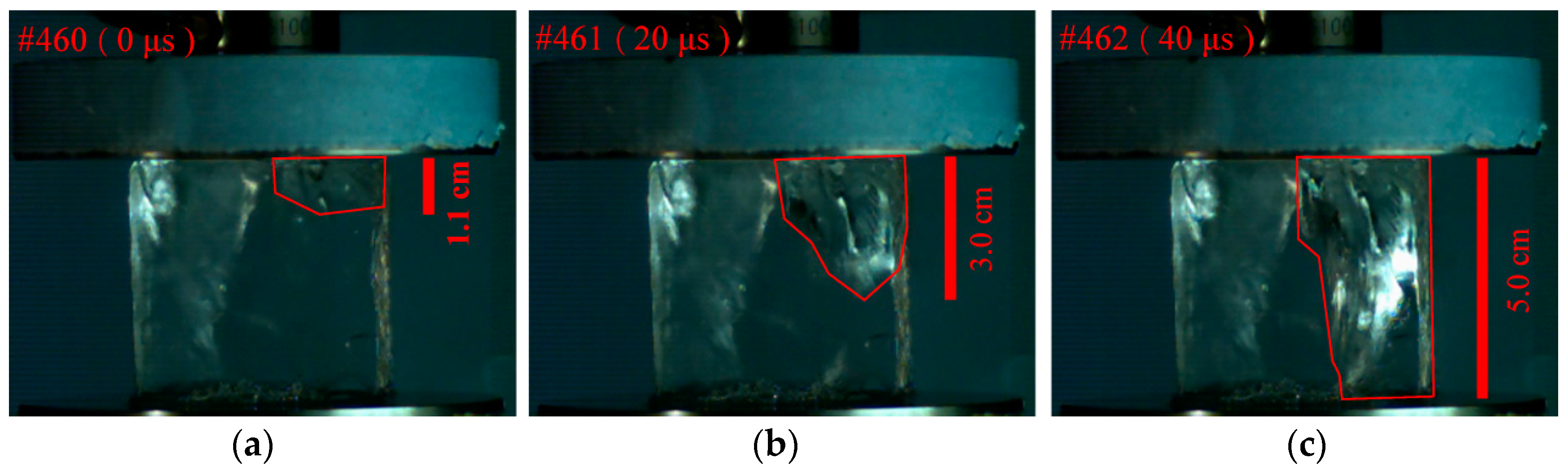
4.4. Crack Propagation Velocity

Failure process of transparent ice samples are recorded by using of a high-speed camera, so it is possible to roughly estimate crack propagation velocity through tracking cracks. Three sequence frames of a hard ice sample in failure process are shown in Figure 20. The loading rate is 0.5 m·s⁻¹ and the loading direction is along the length of the columns. The cracks forming at the right side of ice sample propagate downward. At the time of 0, 20 and 40 μs, the corresponding cracks front are about 1.1, 3.0 and 5.0 cm away from the upper-end of ice sample, respectively. Thus, the crack propagation velocity is approximately 1000 m·s⁻¹. This value is similar to those observed by Pernas-Sánchez et al. [15] and Combescure et al. [11].

5. Conclusions

In this study, a specially-developed high-speed Instron loading system is adopted to perform high-speed compression tests on natural lake ice, combining a two-load-cell system for dynamic load measurement, and a digital speckle correlation method for deformation measurement. According to results of present experiments, the following general conclusions can be drawn:

(1)

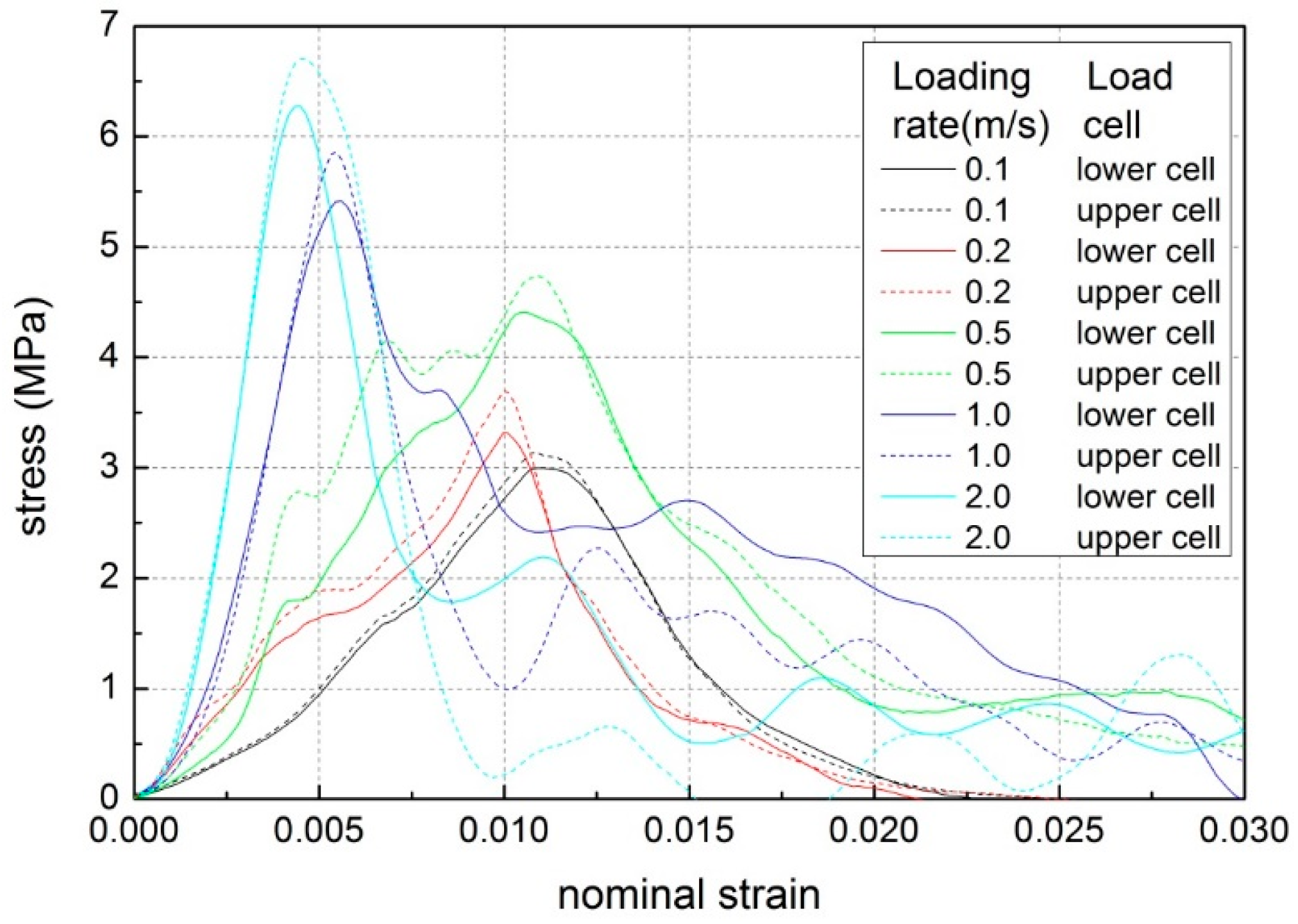
When loading rate is not greater than 2.0 m·s⁻¹, the forces obtained at the two ends of a five-centimeter-high ice specimen are balanced or approximately balanced. Therefore, the difference in forces between the upper-end and the lower-end, resulting from the inertial effect, could be ignored.

(2)

In ice dynamic compression experiments, there may exist a significant difference between true deformation and nominal deformation, so it is not recommended to regard nominal strain-rate and nominal ultimate strain directly as true strain-rate and true ultimate strain.

(3)

By constructing an artificial speckle on ice surface, it is feasible to measure the deformation of ice specimen under dynamic compression tests through the digital speckle correlation method.

(4)

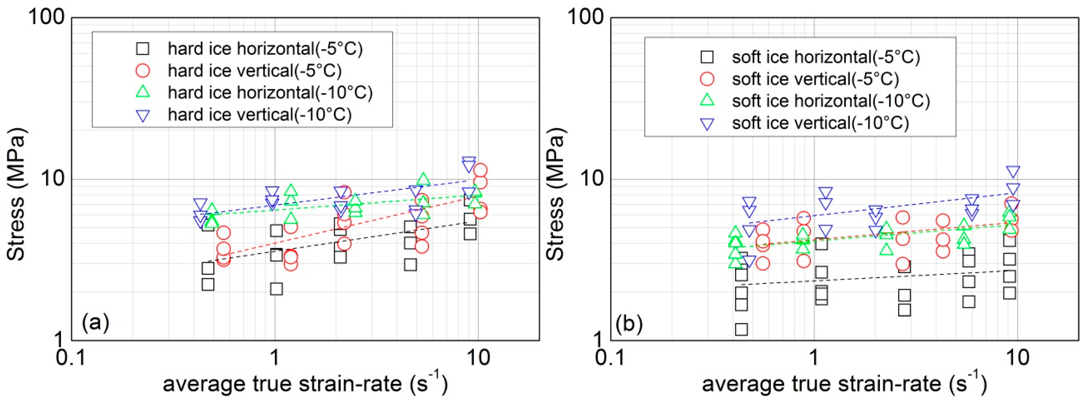
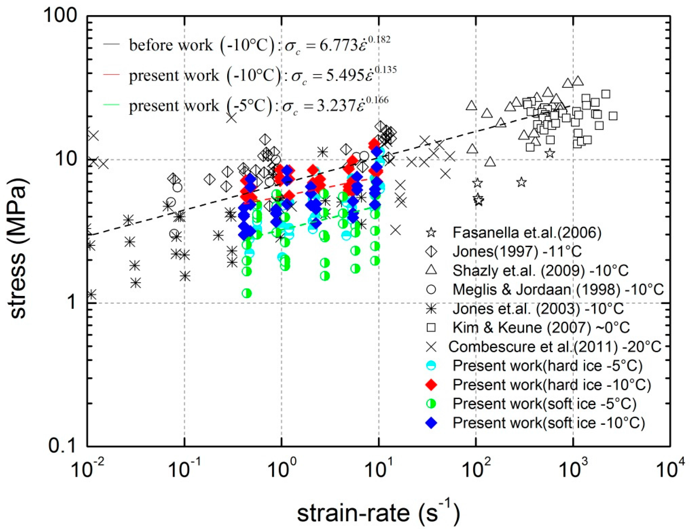
In the employed strain-rate range (0.4–10 s⁻¹), the relationships between uniaxial compressive strength of natural lake ice and its influencing factors, such as strain-rate, temperature, loading direction, as well as air porosity, are almost similar to that under quasi-static conditions. The compressive strength increases with increasing strain-rate, and they obey a power-law relationship with the power exponent of 0.14–0.17. Temperature has a significant effect on the compressive strength, no matter whether the air porosity in ice is low or high and whether the loading direction is horizontal or vertical. The compressive strength shows an increasing trend with decreasing temperature. The strength at −10 °C is about 1.4–1.8 times that at −5 °C. Moreover, the vertical compressive strength is slightly greater than the horizontal compressive strength.

(5)

In the employed strain-rate range, the fracture mode of ice is not sensitive to the loading rate and loading direction. Failure of ice specimen exhibits features of longitudinal splitting failure, accompanied with feature of forming a large number of small fragments, just like that in crushing failure mode. The fracture mode is a combination of splitting failure and crushing failure.

References

1. Michel, B. Ice Mechanics; University of Laval Press: Quebec, QC, Canada, 1978. [Google Scholar]
2. Dempsey, J.P. Research trends in ice mechanics. Int. J. Solids Struct. 2000, 37, 131–153. [Google Scholar] [CrossRef]
3. Cole, D.M. The microstructure of ice and its influence on mechanical properties. Eng. Fract. Mech. 2001, 68, 1797–1822. [Google Scholar] [CrossRef]
4. Schulson, E.M.; Duval, P. Creep and Fracture of Ice; Cambridge University Press: Cambridge, UK, 2009; Volume 1. [Google Scholar]
5. Jones, S.J. High strain-rate compression tests on ice. J. Phys. Chem. B 1997, 101, 6099–6101. [Google Scholar] [CrossRef]
6. Meglis, I.; Jordaan, I. High Speed Testing of Freshwater Granular Ice; Technical Report; National Research Council Canada, Institute for Marine Dynamics: St. John’s, NL, Canada, 1998. [Google Scholar]
7. Jones, S.J.; Gagnon, R.; Derradji, A.; Bugden, A. Compressive strength of iceberg ice. Can. J. Phys. 2003, 81, 191–200. [Google Scholar] [CrossRef]
8. Dutta, P.K.; Cole, D.M.; Schulson, E.M.; Sodhi, D.S. A fracture study of ice under high strain rate loading. Int. J. Offshore Polar Eng. 2004, 14, 182–188. [Google Scholar]
9. Kim, H.; Keune, J.N. Compressive strength of ice at impact strain rates. J. Mater. Sci. 2007, 42, 2802. [Google Scholar] [CrossRef]
10. Shazly, M.; Prakash, V.; Lerch, B.A. High strain-rate behavior of ice under uniaxial compression. Int. J. Solids Struct. 2009, 46, 1499–1515. [Google Scholar] [CrossRef]
11. Combescure, A.; Chuzel-Marmot, Y.; Fabis, J. Experimental study of high-velocity impact and fracture of ice. Int. J. Solids Struct. 2011, 48, 2779–2790. [Google Scholar] [CrossRef]
12. Wu, X.; Prakash, V. Dynamic strength of distill water and lake water ice at high strain rates. Int. J. Impact Eng. 2015, 76, 155–165. [Google Scholar] [CrossRef]
13. Wu, X.; Prakash, V. Dynamic compressive behavior of ice at cryogenic temperatures. Cold Reg. Sci. Technol. 2015, 118, 1–13. [Google Scholar] [CrossRef]
14. Fasanella, E.L.; Boitnott, R.L.; Kellas, S. Test and Analysis Correlation of High Speed Impacts of Ice Cylinders. In Proceedings of the 9th International LS-DYNA Users Conference, Dearborn, MI, USA, 4–6 June 2006. [Google Scholar]
15. Pernas-Sánchez, J.; Artero-Guerrero, J.A.; Varas, D.; López-Puente, J. Analysis of ice impact process at high velocity. Exp. Mech. 2015, 55, 1669–1679. [Google Scholar] [CrossRef]
16. Schulson, E.M. Brittle failure of ice. Eng. Fract. Mech. 2001, 68, 1839–1887. [Google Scholar] [CrossRef]
17. Iliescu, D.; Baker, I.; Cullen, D. Preliminary microstructural and microchemical observations on pond and river accretion ice. Cold Reg. Sci. Technol. 2002, 35, 81–99. [Google Scholar] [CrossRef]
18. Sutton, M.A.; Orteu, J.J.; Schreier, H. Image Correlation for Shape, Motion and Deformation Measurements: Basic Concepts, Theory and Applications; Springer Science & Business Media: New York, NY, USA, 2009. [Google Scholar]
19. Michel, B.; Ramseier, R. Classification of river and lake ice. Can. Geotech. J. 1971, 8, 36–45. [Google Scholar] [CrossRef]
20. Jones, S.J. A review of the strength of iceberg and other freshwater ice and the effect of temperature. Cold Reg. Sci. Technol. 2007, 47, 256–262. [Google Scholar] [CrossRef]
21. Pan, H.; Render, P. Effects of target curvature on the impact characteristics of simulated hailstones. Proc. Inst. Mech. Eng. Part G J. Aerosp. Eng. 1997, 211, 81–90. [Google Scholar] [CrossRef]
22. Samanta, S. Dynamic deformation of aluminium and copper at elevated temperatures. J. Mech. Phys. Solids 1971, 19, 117–135. [Google Scholar] [CrossRef]
23. Gorham, D. Specimen inertia in high strain-rate compression. J. Phys. D Appl. Phys. 1989, 22, 1888–1893. [Google Scholar] [CrossRef]
24. Chu, T.; Ranson, W.; Sutton, M.A. Applications of digital-image-correlation techniques to experimental mechanics. Exp. Mech. 1985, 25, 232–244. [Google Scholar] [CrossRef]
25. Davis, L.A.; Stewart, S.E.; Carsten, C.G.; Snyder, B.A.; Sutton, M.A.; Lessner, S.M. Characterization of fracture behavior of human atherosclerotic fibrous caps using a miniature single edge notched tensile test. Acta Biomater. 2016, 43, 101–111. [Google Scholar] [CrossRef] [PubMed]
26. Koohbor, B.; Kidane, A.; Lu, W.-Y.; Sutton, M.A. Investigation of the dynamic stress–strain response of compressible polymeric foam using a non-parametric analysis. Int. J. Impact Eng. 2016, 91, 170–182. [Google Scholar] [CrossRef]
27. Bartelmo, S.; Rajan, S.; Li, N.; Sutton, M.; Rizos, D.C. Digital Image Correlation Techniques for Prestressed Concrete Tie Quality Control. In Proceedings of the 2016 Joint Rail Conference, Columbia, SC, USA, 12–15 April 2016. [Google Scholar]
28. Sutton, M.; Turner, J.; Chao, Y.; Bruck, H.; Chae, T. Experimental investigations of three-dimensional effects near a crack tip using computer vision. Int. J. Fract. 1992, 53, 201–228. [Google Scholar]
29. McNeill, S.; Sutton, M.; Miao, Z.; Ma, J. Measurement of surface profile using digital image correlation. Exp. Mech. 1997, 37, 13–20. [Google Scholar] [CrossRef]
30. Ma, S.-P.; Jin, G.-C. New Correlation Coefficients Designed for Digital Speckle Correlation Method (DSCM). In Proceedings of the Optical Technology and Image Processing for Fluids and Solids Diagnostics, Bellingham, WA, USA, 3–6 Semptember 2002; pp. 25–33. [Google Scholar]
31. Bruck, H.; McNeill, S.; Sutton, M.A.; Peters, W.H. Digital image correlation using newton-raphson method of partial differential correction. Exp. Mech. 1989, 29, 261–267. [Google Scholar] [CrossRef]
32. Sutton, M.A.; McNeill, S.R.; Jang, J.; Babai, M. Effects of subpixel image restoration on digital correlation error estimates. Opt. Eng. 1988, 27, 870–877. [Google Scholar] [CrossRef]
33. Schulson, E. The brittle compressive fracture of ice. Acta Metall. Mater. 1990, 38, 1963–1976. [Google Scholar] [CrossRef]
34. Yu, T.-L.; Wang, J.-F.; Du, F.; Zhang, L.-Y. Experimental research on ice disaster in huma river. J. Nat. Dis. 2007, 16, 43–48. [Google Scholar]
35. Timco, G.; Frederking, R. Compressive strength of sea ice sheets. Cold Reg. Sci. Technol. 1990, 17, 227–240. [Google Scholar] [CrossRef]
36. Timco, G.; Frederking, R. Seasonal compressive strength of beaufort sea ice sheets. In Ice-Structure Interaction; Springer: Berlin, Germany, 1991; pp. 267–282. [Google Scholar]
37. Manley, M.; Schulson, E. On the strain-rate sensitivity of columnar ice. J. Glaciol. 1997, 43, 408–410. [Google Scholar] [CrossRef]
Figure 1. (a) Hard ice harvested during the stable freezing season and does not contain naked-eye visible air bubbles, with an average air porosity of 0.1%; and soft ice ((b) vertical view; and (c) side view) harvested in early melting reason and contains lots of slender air bubbles, with an average of air porosity of 2.0%.
Applsci 07 00495 g001
Figure 2. Two loading directions: (a) Horizontal loading, i.e., loading perpendicular to the length of the columns; and (b) Vertical loading, i.e., loading along the length of the columns.
Applsci 07 00495 g002
Figure 3. Three types of ice specimens: (a) Non-speckle specimen (transparent specimen); (b) pure-white specimen; and (c) white-black speckle specimen. All of them are cubes with an edge length of 5 cm.
Applsci 07 00495 g003
Figure 4. Schematic sketch of the dynamic loading system and image acquisition system. Two-load-cell monitoring system is shown in the lower right corner.
Applsci 07 00495 g004
Figure 5. Actuator velocity versus time profiles (shown as dotted lines) and load versus time profiles at different loading rates (shown as solid lines). Each intersection points of two kinds of profiles is located in the quasi-horizontal section of the corresponding actuator velocity profile, indicating each ice samples is loaded at an approximately constant loading rate.
Applsci 07 00495 g005
Figure 6. Schematic sketch of the two-dimensional digital speckle correlation method: (a) un-deformed image; and (b) deformed image. P is a reference point.
Applsci 07 00495 g006
Figure 7. Typical speckle field on the ice specimen surface: (a) entire gray-scale image; (b) speckle image; and (c) pseudo-color image of the speckle field. The speckle size in present experiments is 8–15 pixels.
Applsci 07 00495 g007
Figure 8. Typical stress versus nominal strain-rate profiles of hard ice at different loading rates at −10 °C. (Results derived from upper load cell are shown in dot lines and results derived from lower load cells are shown in solid lines).
Applsci 07 00495 g008
Figure 9. Failure processes of hard ice at moderate rates: (a,b) the horizontal loading failure processes of hard ice; and (c,d) the vertical loading failure processes of hard ice. The recording rate of high-speed camera is 50,000 fps.
Applsci 07 00495 g009aApplsci 07 00495 g009b
Figure 10. Stress versus nominal strain profile of sample HH05mps2 at −10 °C (A, B, C, and D denote specific moments, corresponding to time point 0, 0.38, 0.85 and 1.26 ms, respectively).
Applsci 07 00495 g010
Figure 11. Lattice of reference points (the number of reference points is 1804; the spacing between the adjacent reference points is 3 pixels; the reference subzone is a square of 21 pixels in each edge, and the object subzone is four times the size of reference subzone).
Applsci 07 00495 g011
Figure 12. Results of DSCM of sample HH05mps2: (a1a4) Strain in the y-direction; and (b1b4) strain in the x-direction by the digital speckle correlation method (from top to bottom, figures correspond to time point 0, 0.38, 0.85 and 1.26 ms, respectively).
Applsci 07 00495 g012aApplsci 07 00495 g012b
Figure 13. Average true strain-rate versus image NO profiles of sample HH05mps2 at −10 °C: (a) y-direction true strain-rate; and (b) x-direction true strain-rate.
Applsci 07 00495 g013
Figure 14. Typical stress versus nominal strain-rate profiles of soft ice with different loading rates at −5 °C (results derived from the upper load cell are shown as dotted lines and results derived from the lower load cell are shown as solid lines).
Applsci 07 00495 g014
Figure 15. Failure processes of soft ice at moderate rates: (a,b) the horizontal loading failure process of soft ice; and (c,d) the vertical loading failure process of soft ice. The recording rate of high-speed camera is 50,000 fps.
Applsci 07 00495 g015
Figure 16. Relationship between the true deformation and the nominal deformation under dynamic loading conditions: (a) scatter plot of true strain-rate versus nominal strain-rate; and (b) scatter plot of true ultimate strain versus the nominal ultimate strain.
Applsci 07 00495 g016
Figure 17. Uniaxial compressive strength results at moderate strain rates: (a) hard ice; and (b) soft ice.
Applsci 07 00495 g017
Figure 18. Uniaxial compressive strength results of present and some previous work. Solid marks denote results of the present work and hollow marks denote results of some previous studies of other researchers.
Applsci 07 00495 g018
Figure 19. Schematic sketch of the ice fracture mode at moderate strain rates: (a) cracks emerge; (b) cracks propagate vertically or approximately vertically; (c) several vertical full-height cracks appear; (d) forming quantities of intersection and link-up among cracks, and reaching peak load; (e) expanding obviously; and (f) crushing into small fragments.
Applsci 07 00495 g019
Figure 20. Sequence frames of a 5.0-centimeter-high ice sample in failure process, loaded vertically at a rate of 0.5 m·s−1 and recorded at a frame rate of 50,000 fps: (a) #460; (b) #461; (c) #462.
Applsci 07 00495 g020