
Damage Assessment Using Information Entropy of Individual Acoustic Emission Waveforms during Cyclic Fatigue Loading

Center for Risk and Reliability, Department of Mechanical Engineering, University of Maryland, 2181 Glenn L. Martin Hall, 4298 Campus Dr., College Park, MD 20742, USA
*
Author to whom correspondence should be addressed.
Appl. Sci. 2017, 7(6), 562; https://doi.org/10.3390/app7060562
Submission received: 24 February 2017
/
Revised: 25 May 2017
/
Accepted: 25 May 2017
/
Published: 30 May 2017
(This article belongs to the Special Issue Advances in Acoustic Emission and Health Monitoring of Materials and Structures)
Abstract
:Featured Application
The work presented in this paper outlines three methods to analyze individual acoustic emission waves emitted within a cyclically-loaded metallic structure. Upon further development, one potential application of the proposed analysis methods would be to aid in estimating the remaining useful life of aircraft structures.
Abstract
Information entropy measured from acoustic emission (AE) waveforms is shown to be an indicator of fatigue damage in a high-strength aluminum alloy. Three methods of measuring the AE information entropy, regarded as a direct measure of microstructural disorder, are proposed and compared with traditional damage-related AE features. Several tension–tension fatigue experiments were performed with dogbone samples of aluminum 7075-T6, a commonly used material in aerospace structures. Unlike previous studies in which fatigue damage is measured based on visible crack growth, this work investigated fatigue damage both prior to and after crack initiation through the use of instantaneous elastic modulus degradation. Results show that one of the three entropy measurement methods appears to better assess the damage than the traditional AE features, whereas the other two entropies have unique trends that can differentiate between small and large cracks.
1. Introduction
Decades of research have produced guidelines for estimating ideal service life for aircraft to limit safety risks and monetary losses due to catastrophic fatigue failure. Specifically, the United States Navy uses the safe-life approach and retires aircraft once a crack is estimated to initiate and extend to a length of 0.25 mm based on extensive and time-consuming full-scale fatigue tests [1]. While the relatively low damage threshold of the safe-life approach reduces the likelihood of failure, the high safety factors tend to lead to premature retirement and a lower return on investment for aircraft owners [2]. Rather than basing retirement time solely on estimated crack initiation and full-scale testing, structural health monitoring (SHM) and nondestructive evaluation (NDE) methods can be used to estimate the true fatigue damage in a material. While SHM is most desirable in that the entire structural health is continuously monitored, NDE methods that evaluate structural health during discrete inspection periods are more practical and often implemented.
Acoustic emission (AE) has become a recognized NDE method for detecting flaws in mechanically loaded structures. When a cyclic stress is applied to a metallic structure, dislocations move and create microcracks near inclusions which coalesce to form macrocracks. These defects are considered to cause disorder within the structure, and, thus, fatigue damage is considered to be synonymous with microstructural disorder. During this growing microstructural disorder, stored elastic strain energy is released partly in the form of acoustic waves that can be measured and analyzed [3]. In the past, researchers have correlated AE signals to large fatigue crack propagation in metals. A popular method for doing so has been to correlate the number times the AE voltage signal crosses a certain amplitude threshold, referred to as counts, and the crack growth rate using a power law relationship [4,5,6,7,8,9,10,11,12,13]. In addition, other AE features have been studied as fatigue cracks grow, such as amplitude [11,12,14,15], energy [14,15], rise time [11,15,16,17], and average frequency [15,16,17]. While methods for estimating stable crack growth rate based on AE signals are well established, estimating crack damage at the smallest possible scale is most desirable. This idea has motivated researchers to better understand wave dynamics of AE signals within single crystals [18,19,20,21] and polycrystalline materials [11,12,15,22,23,24,25,26,27,28,29,30] (see [31] for further discussion on past AE literature). From these studies, researchers concluded that AE activity is present during initial damage due to dislocation motion and microcracks, and various AE features can be correlated to damage.
Rather than using AE features as descriptors of fatigue damage and microstructural disorder, one can measure the actual disorder or the information content of the received AE signals using information entropy. Various methods to quantify the information entropy in the AE signals have been previously proposed. Unnthorsson and colleagues [32] estimated two time-domain entropies and two frequency-domain entropies from AE signals recorded during composite fatigue tests. The entropies were calculated from discrete probability distributions of the amplitude and frequency measured for one fatigue cycle every five minutes of testing. In the end, the entropy evolutions were similar to AE count trends, and entropy from AE signals was proposed to be a measure of microstructural disorder. Reference [33] also focused on deriving entropy from AE amplitude distributions as a measure of fatigue damage. Results showed that measured disorder from AE amplitude distributions increased as damage also increased. Ramasso et al. [34] introduced unsupervised pattern recognition based on time and frequency in order to distinguish clusters of AE signals and computed mutual entropy. Finally, Amiri and Modarres [35], and Kahirdeh, et al. [36] have estimated the entropy from AE counts during fatigue tests of aluminum and titanium alloys. It was shown that information entropy derived from the AE counts mirrored the evolution of counts throughout the tests [35], and the cumulative information entropy from counts may be constant at failure [36].
For all of these previous studies that estimated information entropy from AE signals, the information entropy was calculated based on AE feature distributions formed from numerous AE signals. Instead of analyzing features from several AE hits at a time, one can estimate the information entropy of each individual AE waveform from the signals’ voltage distributions. This technique theoretically utilizes more information carried in an AE signal compared to summary statistics like counts, amplitude, or average frequency and is expected to be a more representative measure of fatigue damage. This idea is the fundamental basis of the work presented in this paper: to extract information entropy from every individual AE signal during fatigue tests as a measure of the AE signal disorder and damage within a fatigued structure.
In this paper, we propose three methods to quantify the information entropy from individual AE signals. The entropy values from these three methods, referred to as instantaneous entropy, average entropy, and weighted average entropy, are derived from AE signals received during fatigue experiments performed on a commonly used aerospace alloy, Al7075-T6. This work studies information entropy of AE signals both prior to crack initiation and after a crack began to propagate. Unlike previous research in which fatigue damage is easily quantified based on visible crack length, this work assumes that instantaneous elastic modulus can be an estimate of the unobservable microstructural damage before appearance and initiation of a visible crack. AE counts and AE energy, two traditional AE signal features, in addition to the three methods of quantifying information entropy from AE signals, are correlated to modulus degradation throughout crack initiation and growth. Results suggest that employing information entropy from AE waveforms would be more advantageous than utilizing the traditional AE features as fatigue damage measures. The figures provided in this paper can be found in the Supplementary Materials.
2. Information Entropy
2.1. Information Entropy Fundamentals
Information theory began in 1948 with Claude E. Shannon’s [37] proposed information entropy as a measure of disorder or uncertainty in a message calculated based on the following equation:
where S is the information entropy, K is a constant that dictates the entropy units, and p(x) is a probability mass function, where p()is the probability of a certain value, , present within the message with n possible values. It should also be noted that the probabilities need to sum to 1. In addition, let so that the logarithm will have a base of 2 to yield entropy in units of bits [37,38].
To better understand the information entropy of a signal, it is helpful to see examples of calculating information entropy from various probability distributions. Consider the probability distribution of flipping a fair coin. A person flipping this coin has little information and is uncertain about whether the outcome will be heads or tails. Let heads be outcome , tails be outcome , and the probabilities for each outcome be p() = 0.5 and p() = 0.5. From this probability distribution, the information entropy can be calculated based on Equation (1) and is found to be 1.00 bit. This distribution and calculation is depicted in Figure 1a.
Now consider a biased coin that results in tails 70% of the time. A person flipping the coin now has more information and is less uncertain about the possible outcome. A new probability distribution can be constructed to reflect the biased coin, and the entropy of this distribution is less than before, at 0.88 bits as recorded in Figure 1b. Finally, consider a biased coin that is tails 99% of the time when flipped. Knowing this bias, a person flipping the coin would be almost certain that the outcome will be tails. This probability distribution is represented in Figure 1c and results in an even lower entropy value of 0.08 bits. This scenario demonstrates that a more uniform probability distribution representing a highly disordered and more uncertain variable will have a higher information entropy value. In other words, the greater the uncertainty and disorder, the greater the entropy will be.
Given any variable or signal that is represented by a probability distribution, one can calculate information entropy using Equation (1) as a measure of the variable’s disorder or uncertainty. The maximum entropy will be from a distribution with equally likely outcomes, whereas the minimum entropy of 0 bits will be from a deterministic distribution when only one outcome from a sample space is possible.
2.2. Information Entropy of Individual AE Waveforms
The disorder of AE signals with information entropy can be estimated through several different methods. All of the methods developed in this work have one commonality: a probability distribution is formed based on voltage readings in individual AE waveforms. Again, this compares to the AE features such as counts and energy that are acquisition system outputs and which summarize AE waveforms. Because information entropy is a measure of uncertainty about a random variable’s value as described by its probability distribution, the AE information entropy can directly reflect microstructural changes. This idea is exemplified in Figure 2, which depicts three independent AE signals, their waveforms, and voltage distributions. One can infer that Signal A is caused by a less significant microstructural change compared to Signal B and Signal C. As such, the voltage distribution can be formed and the information entropy of these distributions can be calculated based on Equation (1). Thus, it is evident that an AE signal believed to reflect a larger microstructural change will have a greater entropy value.
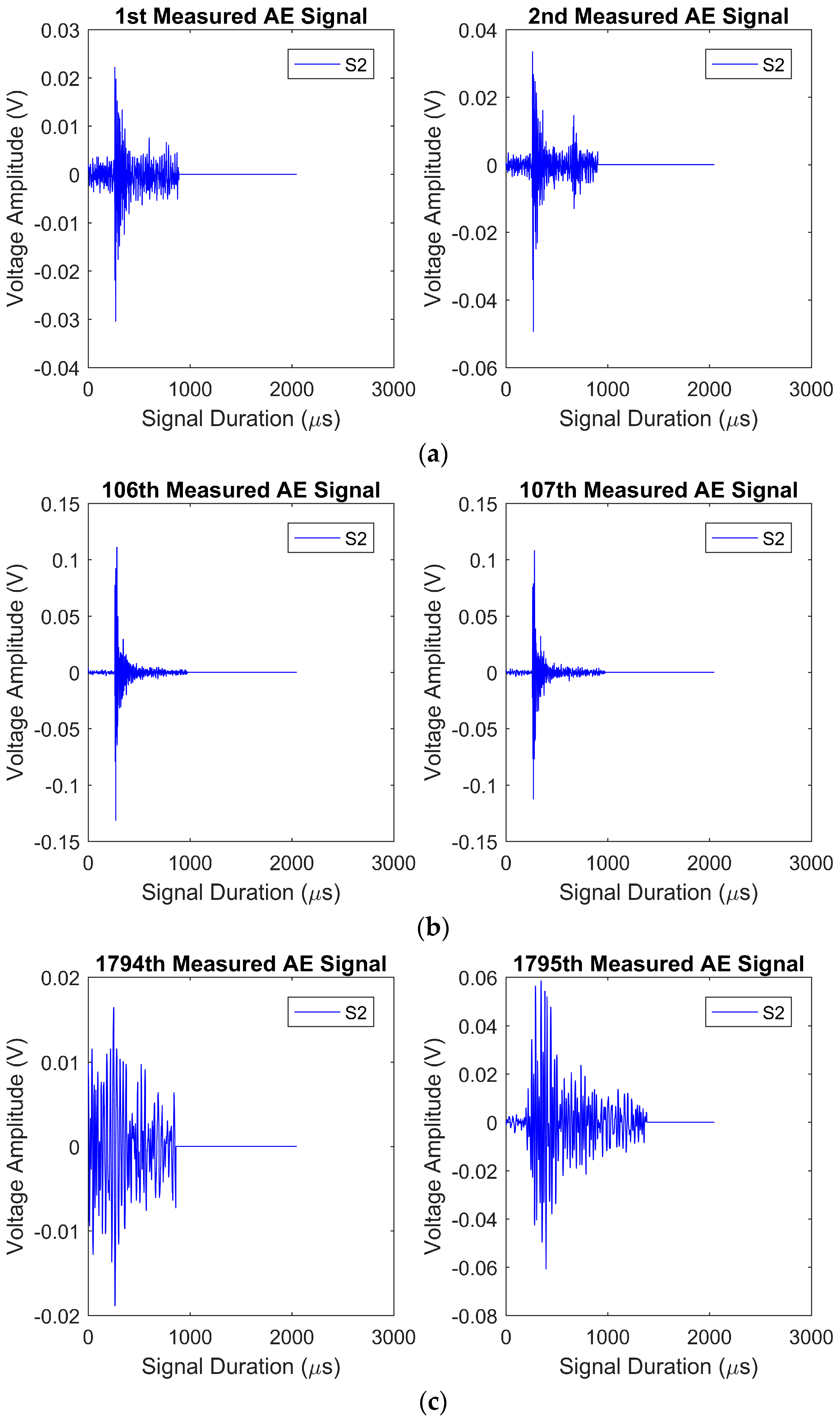
It must be noticed that the shape and characteristics of the AE signals varies depending on the degradation stage of the experiment. In order to visualize the change in the shape of the acoustic emission signals, six signals are demonstrated in Figure 3. Figure 3a depicts the first two signals that are measured in the test S1 (we call experiments 1–8 as S1–8). These two signals are measured during the deformation of the sample. The next two signals that are demonstrated in Figure 3b correspond to the instant of crack initiation in the test S2. It has been observed that such signals have a sharp peak comparing to the Figure 3a. The signals received in the beginning of the test and instant of crack initiation are burst type signal. However, continuous types of emissions are measured at the time of fracture of the specimen, which is depicted in Figure 3c. The last two acoustic emission signals are measured in the course of the fatigue test, S2.
There are two general steps for estimating information entropy from AE signals regardless of the method. A probability distribution of the random variable describing the AE signals must first be formed, and then the amount of disorder exhibited by the distribution via Equation (1) must be quantified. In this case, the chosen random variable is the signal amplitude expressed in units of voltage where the AE voltage probability distribution represents the microstructural disorder, and the distribution is evolving as fatigue damage progresses.
During the early part of a fatigue experiment, the “true” AE voltage probability distribution is completely unknown until a first AE signal is recorded. Let this AE signal be described by its 2048 voltage readings, which are 2048 samples from the current underlying voltage probability distribution. Because the true AE voltage probability distribution is unknown, an imprecise distribution is estimated from these 2048 voltage values. The disorder of this distribution is then quantified by Equation (1). When a second AE signal is received, the new set of 2048 voltage values provides new information about the voltage probability distribution and needs to be considered. Three different methods to account for this new information about the probability distribution have been investigated and yield three formulations to derive AE information entropy.
First, one can assume that the underlying AE voltage distribution is constantly changing and is independent between all the time steps. Therefore, a new probability distribution of the second AE signal’s 2048 voltage values should be created to estimate the true distribution at that particular instant. With every new AE signal, a new probability distribution is constructed to represent the constantly-changing underlying distribution. The information entropy calculated from each of these distributions is referred to as instantaneous entropy.
The second method is based on the theory that the underlying probability distribution changes very slowly, and the second AE signal received is from approximately the same distribution as the first AE signal. In turn, the 2048 voltage values from the first and second signal are combined, and a distribution is formed from the total 4096 voltage values. As more AE signals are received, all of the new and previous AE voltage values are concatenated, and the estimated probability distribution of the true underlying distribution is updated for each new AE signal. Another way to explain this process is that every AE signal’s distributions are combined and have equal effect on the estimated distribution. Because each received AE signal has an equal weight on the voltage distribution, the information entropy calculated from these updated distributions is referred to as average entropy.
Finally, the third method is based on a slowly-evolving true probability distribution of AE voltage values similar to average entropy, but assumes more recent AE signals better represent the underlying distribution than past AE signals. When a second AE signal is received, a distribution of the 2048 voltage values is formed similarly to the procedure for instantaneous entropy. Then, the first and second signals’ distributions are combined so that the more recent signal’s distribution is weighted more than the previous. When subsequent AE signals are received, new distributions are formed where the most recent AE signal has the greatest weight on the updated distribution. The specific weights are determined based on the signal arrival times and are calculated using the following equation:
where the weight vector, w, and arrival time vector, , are 1 × n vectors and n is the current number of recorded AE signals. For example, if the first AE signal occurs at 2 s and the second is recorded at 4 s, then the first signal’s distribution will have one-half of the weight of the second signal’s distribution. The information entropy calculated from these weighted and updated distributions is referred to as weighted average entropy. In the end, instantaneous entropy, which produces independent entropy values, is the most erratic; average entropy has the most inertial trend; and weighted average entropy is similar to average entropy with more significance placed on current signal’s instantaneous entropy. An example Matlab script that calculates these three entropy values for a set of AE signals is provided in the Supplementary Materials.
3. Materials and Methods
3.1. Specimens
Specimens used for this study were aluminum alloy 7075-T6. The material’s composition and mechanical properties are presented in Table 1. The raw material was machined into dogbone specimens designed according to ASTM standard E466 [39]. A 1-mm radius edge notch is located at the center of the gauge length and acts as a stress concentrator. This intentional flaw ensures that fatigue damage and crack initiation will occur at this location with a stress concentration factor of 2.61 [40]. Once the specimens were machined, one side of the specimen’s gauge length was polished with fine grit sandpaper and 3 µm alumina solution followed by etching. In turn, the propagating crack could be seen clearly under magnification during fatigue loading. The experimental setup is depicted in Figure 4.
3.2. Instrumentation
Fatigue experiments were performed with loading ratio of 0.1 and loading frequency of 5 Hz. A servo-hydraulic Materials Testing System (MTS) machine retrofitted with an Instron 8800 controller was used to perform the fatigue tests. The maximum applied load varied between 8 and 15 kN. The theoretical maximum applied stress can be estimated by dividing the load by the gauge length cross-sectional area, 57.15 mm2, and multiplying by the stress concentration factor, 2.61, yielding estimated applied stresses between 480 and 685 MPa. The strain around the edge notch was measured with an Epsilon 3542 extensometer with a gauge length of 25 mm. To prevent sliding or rubbing on the specimen, rubber bands were used to fasten the extensometer to the specimen’s face. An optical microscope with an attached time-lapse camera captured images every 25 cycles to monitor the initiation of a crack and its growth from one side of the specimens. Crack initiation was recorded as the first instance a crack was visible on this one face and, because the cracks could have initiated on the other face not monitored by the microscope, there is some uncertainty in the crack initiation time and small crack length. However, it is assumed that once the crack reached 1 mm as measured on the monitored specimen face, the crack is of sufficient length to have propagated through the specimen thickness.
AE signals were recorded with a PCI-2 based AE system supplied by the MISTRAS Group (Princeton Junction, NJ, USA). Two resonant Micro30s AE sensors with a frequency range of 150–400 kHz and resonant frequency of 225 kHz were used. A sampling rate of 1 MSPS was used to capture the signals. According to the Nyquist–Shannon sampling theorem, frequencies up to 1/2 of the sampling frequency meaning up to 500 kHz were distinguishable. However, signal frequencies at the top of the frequency range of the sensor are considered unreliable at this sampling rate. If other AE sensors with higher operating frequency ranges were to be used, the sampling frequency would have to be increased accordingly.
The sensors were mounted to one side of the specimen 23 mm above and below the center of the notch. Ultrasonic gel was used as a couplant, and electrical tape fastened the sensors to the surface. The AE signals passed through a 40 dB preamplifier before reaching the data acquisition module where AEwin software then plotted and extracted the AE signals. The AE acquisition system also received load and extension data as analog inputs from the testing machine. This feature enabled the AE signals to be paired with the applied load and is crucial to post-process filtering described in Section 3.3. Other user-defined settings that control how the AE signals are collected are summarized in Table 2. These parameters were selected based on pencil lead break tests [41], a common standard that produces repeatable artificial AE waves with similar characteristics to damage-related AE signals. The AE sensors and crack growth monitoring system are shown in Figure 4.
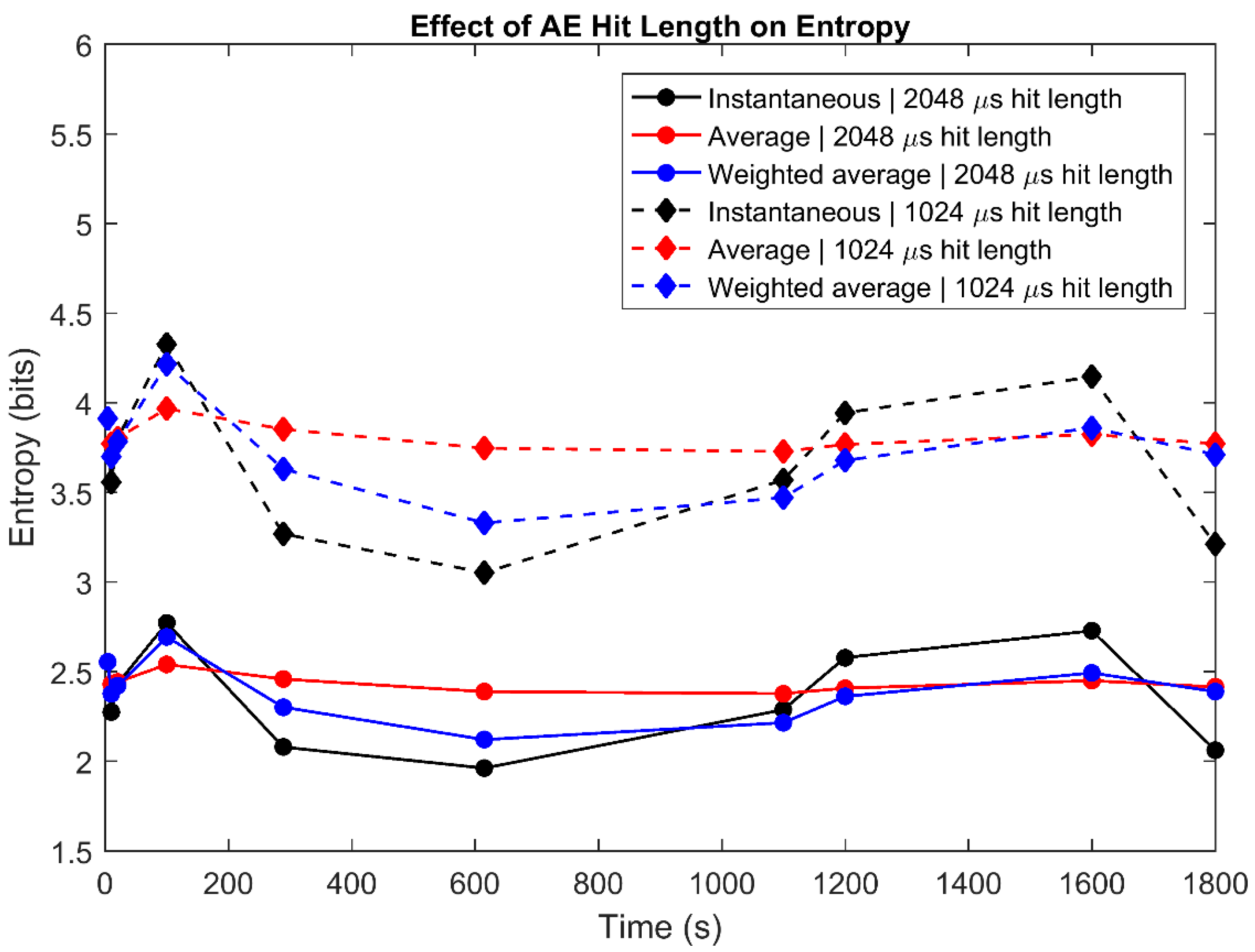
It should be noted that the values of entropy from AE signals would change if any of the acquisition parameters were altered. However, the trends in entropy measures between the AE signals throughout a fatigue experiment would not change. For example, Figure 5 shows the instantaneous, average, and weighted average entropy for 10 signals plotted versus time where the first set is for a hit length of 2048 microseconds and the second set is for a hit length of 1024 microseconds. This chart shows that, while the values of entropy are higher for a shorter hit length, the trends in these entropies between AE signals do not change. Thus, the conclusions made from the waveforms collected with these acquisition parameters are applicable to waveforms collected with different parameters.
3.3. Noise Reduction
Servo-hydraulic machines are known to produce AE background noise of similar frequency and amplitude to damage-related AE signals making filtering the noise a difficult process. In order to reduce the noise effects, so-called filtering methods have been developed with various approaches [13,24,26,28,34,42,43,44,45]. The methods can be classified into pre- and post-processes. Pre-process prevents noise by using mechanical damper [42] or maps the AE signal source location by using multiple sensors and collects signals from the region of interest [28]. Post-process is filtering AE signals based on specific features such as instantaneous loading [45] or partitions AE clusters [42,43,44]. When AE signals are distinguished by load, higher load [4,10,12,26] or lower load [44,45] is chosen for meaningful signals. As another approach, AE signals are separated by loading and unloading periods [45].
Aligned with known pre-processing noise reduction techniques, filtering of AE signals based on signal arrival times [28] and on frequency [13,26] was attempted, but neither of these methods have proven effective for this particular test setup. Specifically, the technique of locating AE sources within the specimens based on signal arrival times between two or more sensors would allow a user to reject AE signals that emitted from sources located away from the notch. This method theoretically would allow the user to set the AE threshold at a lower level where noise signals are collected along with damage-related signals, and then the signals would be filtered based on their source location. This technique proved successful during pencil lead break tests. However, when the method was applied for during cyclic loading and the threshold was set to a level that would allow collection of noise signals, the acquisition system was overloaded and ceased to function. The noise signals and damage-related signals also proved to have indistinguishable frequency spectrums, and filtering signals based on frequency could not be simply employed. Instead, in this research attempts were made to actively limit the noise signals from propagating through the specimens and to filter identified noise-related AE signals during post processing.
First, the background noise amplitude, which reached as high as 65 dB in preliminary experiments, was reduced by a mechanical damping apparatus inspired from Miller’s work [42]. After testing several different materials and configurations, the final apparatus consisted of four sets of clamped, 1/4 inch thick, styrene-butadiene rubber blocks and four tightly-wrapped, 1/16 inch thick, neoprene strips attached to areas between the testing grips and specimen gauge length. These elastomers, shown in Figure 4, inhibited mechanical vibration and reduced the background noise by as much as 20 dB. In the end, AE signals from the AE sensor located above the notch were used for analysis because the threshold could be set to 45 dB with ease. Signals from the lower sensor were used only to validate the upper sensor’s behavior because noise signals of up to 48 dB were detected by this sensor even with the mechanical damping apparatus Thus, the amplitude threshold for the lower sensor was adjusted to 48 dB to avoid overloading the data acquisition system. In turn, the source of the AE signals could not be located but only the AE signal behavior of the upper sensor could be verified.
Despite reducing the AE background noise to amplitudes below 45 dB with the mechanical damping method, AE noise signals were still collected during some tests in the upper sensor. Thus, a filtering technique based on applied load at the instant of AE signals was implemented. This method assumes that the AE signals are sporadically received as microcracks form and will most likely occur when a structure is applied with maximum stress [4,10,12,26]. An example of the expected AE signal behavior with no apparent noise signals is plotted in Figure 6a for experiment S8. This graph shows the AE signals as points at the associated load and time and meets both of the expected criteria. The cumulative hits over time for this experiment is depicted in Figure 6d where a majority of the hits are shown to be acquired near specimen fracture as expected.
However, other experiments showed both the expected AE behavior and another behavior that is believed to be unwanted noise. This unwanted behavior is characterized by AE signals continuously occurring at mid-range loads forming clusters when plotted against their associated load and arrival time. The noise behavior also seems to evolve throughout the fatigue tests where numerous noise signals are suddenly detected after a substantial amount of the specimens’ fatigue lives are depleted and then are not evident after a few cycles. These clusters suggest either that strain energy is released consistently away from the maximum load or that mechanical noise is generated consistently at particular points of the loading cycle. The latter is assumed to be more likely where this noise is believed to be an unfortunate attribute of the hydraulic system that powers the fatigue testing machine, and therefore, these signals were excluded. The scatter plot of applied load at the instant of AE signals for one such test, S4, is pictured in Figure 6b. The cumulative AE hits for this experiment is depicted in Figure 6e. This plots shows that the AE hits assumed to be from the noise clusters create a jagged cumulative hits trend and account for about 40% of the acquired signals. Too many noise signals were recorded for other tests, and the expected AE behavior and noise could not be confidently differentiated. Figure 6c shows the applied load at AE hits versus time for one such test as an example of noise that proved impossible to separate from the assumed damage-related AE hits. Subsequently, the cumulative AE hits over time is shown in Figure 6f where the total hits are over 10 times more than an experiment with no apparent noise, and the trend is close to linear rather than exponential towards the end of the experiment. In the end, the filtering method was kept consistent in that clusters of AE signals at low loads were removed, and tests that would have required questionable noise filtering were not used in the analysis. Further information about the noise reduction processes can be found in [31].
3.4. Modulus Degradation
Material degradation is reflected as a decrease in the structure’s elastic modulus [46]. Dislocations move and microcracks grow such that the material becomes less stiff and will elongate more for the same applied load as damage progresses. The initial elastic modulus close to 67.8 GPa as noted in Table 1 and a consistent modulus degradation trend between specimens is expected. The elastic modulus for each fatigue cycle is approximated by dividing the difference between the maximum and minimum applied nominal stress in the cycle by the difference between the strain at the maximum and minimum stress. While the stress at the notch tip is estimated to be either elastic or plastic between the experiments depending on the applied loading, the nominal stresses for all experiments (between 180 and 270 MPa) are below the yield stress (538 MPa) suggesting that the use of modulus degradation, which is only applicable for the elastic region, is valid. The raw modulus trends can then be normalized and are referred to as modulus degradation damage (MDD). The correlation between AE parameters and this statistic ensures that the variations between the initial and final modulus of the experiments are reduced and allows data from all tests to be analyzed together. An example Matlab script that calculates the elastic modulus for each fatigue cycle is provided in the Supplementary Materials as well as a script that matches AE features to MDD for each cycle. In this case, MDD is calculated based on the following equation:
where Ei is the modulus at each cycle, E0 is the initial modulus, and Ef is the final modulus. An MDD value of 0 refers to a pristine specimen, while 1 is associated with specimen fracture.
Numerous experiments were performed to refine the experimental setup and procedure. In the end, eight experiments with consistent experimental setups and acceptable AE signal behavior were analyzed in regards to modulus degradation and AE signal features. The entire experimental setup is depicted in Figure 4 as previously mentioned.
4. Results and Discussion
4.1. Cumulative Instantaneous Entropy, Counts, and Energy
4.1.1. Comparing Cyclic Evolutions and Values at Fracture
Instantaneous entropy proposed in this work is calculated from AE signals by forming independent and new distributions of each individual AE signal’s voltage values and employing Shannon’s equation to estimate the distributions’ disorders. Because instantaneous entropy is independent between waveforms, the total disorder due to fatigue damage is assumed to be measured by cumulative instantaneous entropy from the AE signals. To assess its utility, cumulative instantaneous entropy can be compared to cumulative counts and cumulative energy. First, it is best to observe the cumulative instantaneous entropy, counts, and energy behaviors against fatigue cycles up until specimen fracture as reported in Figure 7. This figure shows that all cumulative features slightly increase initially, stay constant for the majority of life, and then begin to increase near final fracture. This trend proves to be similar to fatigue stages in which crack growth is relatively constant for almost the entirety of fatigue and then sharply increases once a crack has initiated. In addition, MDD versus cycles for each experiment through fracture is depicted in Figure 8 showing that most of the damage measured via MDD is recorded in the last 2000–4000 cycles.
Another point to consider is the final cumulative values of instantaneous entropy, counts, and energy at fracture. Theoretically, measures of damage should be of the same magnitude between identical structures that have been exhibited to the same level of fatigue loading even though uncertainty is inherent in material’s property and measurements. Thus, any metric that represents the cumulative fatigue damage should be similar for all specimens with cracks of equal lengths and at fracture. Some variations, however, are expected in the final cumulative AE parameters at fracture due to inaccurate classification of AE noise signals, imprecise sensor placement which alters AE signal attenuation, and inherent microstructural differences between specimens.
The spread of the final cumulative values can be quantified by the coefficient of variation (CV). The CV measures the relative standard deviation of a set of random numbers assumed to have come from a normal distribution. The following equation shows the CV in percent calculated based on the sample standard deviation, σ, and the sample mean, µ:
A CV of 0 suggests all values are the same with no variability (i.e., no uncertainties), while wider data scatters will have larger CV values. Results for cumulative AE parameters are recorded in Table 3 where the CV for counts is the lowest at 18.2% followed by energy at 20.2%, while instantaneous entropy has the greatest CV of 22.4%.
These values suggest cumulative instantaneous entropy has the most variability at fracture compared to cumulative counts and cumulative energy. Therefore, one could say instantaneous entropy may be most influenced by random variations in experiments compared to the other two traditional AE features. While it may seem advantageous for a parameter to have a lower CV, the higher variation for instantaneous entropy means that is it more sensitive to slight differences in AE signals. Thus, it could potentially be a better, more sensitive measure of damage if variations between experiments were reduced.
4.1.2. Comparing Damage Trends
Rather than attempting to compare the final values of cumulative AE parameters that have different units, comparisons between the normalized, unitless parameters with respect to MDD can be drawn. The parameters are normalized by the following equation:
where p is any AE parameter so that variabilities between experiments are reduced and metrics are no longer scale-dependent. Based on the cyclic trends, it is expected that each cumulative AE parameter increases more at the beginning and end of damage and increases less for the majority of damage. However, normalized cumulative AE parameters with a constant relationship with MDD would be ideal and suggest “perfect correlation”. Thus, it is assumed that cumulative AE features are best to predict damage if they have a one-to-one relationship on normalized scales.
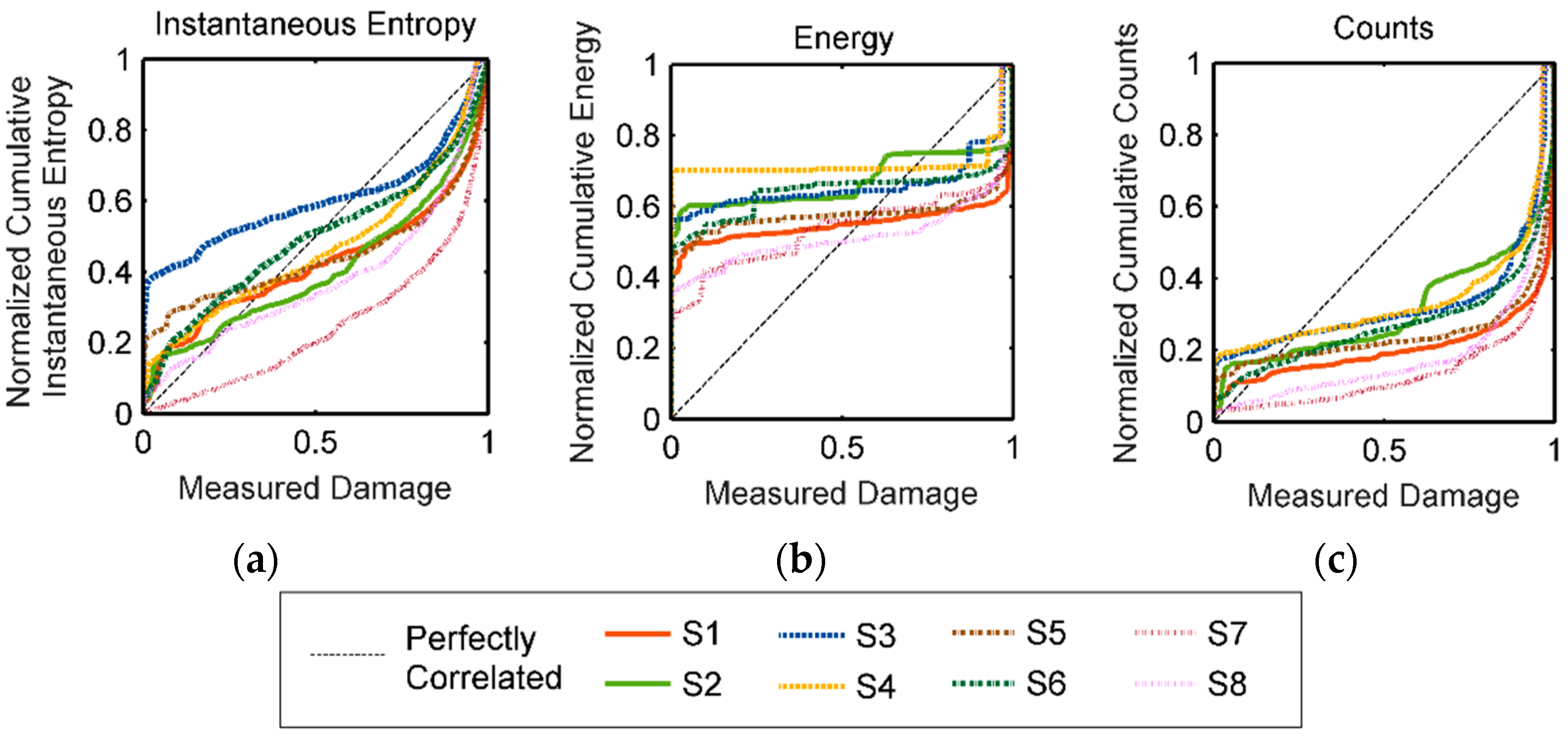
These graphs until specimen fracture along with the desired one-to-one relationship are plotted in Figure 9. All features show a greater increase at the beginning and end of damage compared to the middle damage values and deviate from the ideal relationship. More specifically, about 60% of the total increase in counts occurs near the point of fracture, while about 50% of the cumulative energy occurs at initial damage. This result suggests that counts may be more responsive at the end of fatigue life and energy may be more responsive during initial damage. In contrast, instantaneous entropy seems to be more equally responsive for all fatigue damage stages, meaning instantaneous entropy may be better correlated to damage than counts and energy.
The differences between the cumulative AE parameters damage trends can be quantified by measuring the deviations from the one-to-one ideal relationship. The deviations are measured at each instance of an AE signal. The summation of these deviations, referred to as the deviation factor, can then be used as a goodness of fit metric of the one-to-one model and compared between the AE parameters for each test. The AE parameter with the lowest deviation factor is assumed to be a better representation of damage. It should be noted that only the deviation factors can be compared because all AE features are normalized to the same scale and the number of deviations are equal between parameters for each experiment. The deviation factors for each of the experiments and for each of the cumulative AE parameters were calculated and are plotted in Figure 10. Results show the deviation factor for instantaneous entropy is lower than the deviation factors for counts and energy for all but one experiment. This result further suggests instantaneous entropy may be a better statistic of damage compared to counts and energy.
4.2. Average and Weighted Average Entropy
Rather than measuring and summing the individual disorders from each AE signal with instantaneous entropy, the average entropy and weighted average entropy estimate the true AE voltage distribution by continuously updating the distribution as new AE signals are received. Average entropy weighs all AE signal distributions evenly, while weighted average entropy weighs voltage distributions based on signal arrival time. Because these two methods of deriving entropy are found from a continuously updated distribution that utilizes all currently received AE signals, it is not logical to view these entropies in cumulative forms. Instead, they should be plotted in their singular forms where the value at fracture is not expected to be consistent between experiments.
Average and weighted average entropy are meant to estimate the current distribution of possible AE voltage values. If significant and unique microstructural damage occurs within the structure, then it is expected that AE signals with large voltage amplitudes will be received, and therefore the probability distribution will become wider. In contrast, when small microstructural damages occur and emit small amplitude AE signals, the estimated voltage distribution will become thinner and concentrate at 0 volts.
The trend of average and weighted average entropy can be predicted based on this logic. First, signals received prior to and during crack initiation are assumed to be infrequent due to dislocation pile up [25] and have high disorder from the sudden release of energy when dislocations break away [18]. AE signals are received from numerous locations around the notch, because a crack has not yet initiated and the exact location of crack initiation is uncertain. Therefore, it is hypothesized that the entropies prior to crack initiation will be relatively high-valued and sporadic due to the high energy and inconsistent AE sources. High energy signals are even evident in the first few fatigue cycles as the pristine specimens are stressed for the first time. After a crack begins to initiate, previous work suggests sudden bursts of low amplitude AE signals due to micro-cleavage [25] or due to wave reflections at the extended crack boundary [14] will then be received. It is believed that these frequent and low-disordered AE waveforms are emitted from the particular microcrack leading to macrocrack initiation, rather than from multiple potential crack initiation sources. Thus, the entropy trends are believed to decrease as a crack initiates and begins to grow. Finally, high amplitude AE signals are expected once the crack propagates to a critical length and causes fracture. In turn, entropies will then increase near fracture. Only slight differences between average and weighted average entropy are expected where weighted average entropy would have a more irregular trend than average entropy. The purpose of proposing both average and weighted average entropy is to introduce two possible methods of estimating entropy from an AE signal while considering AE signals received prior to the current signal.
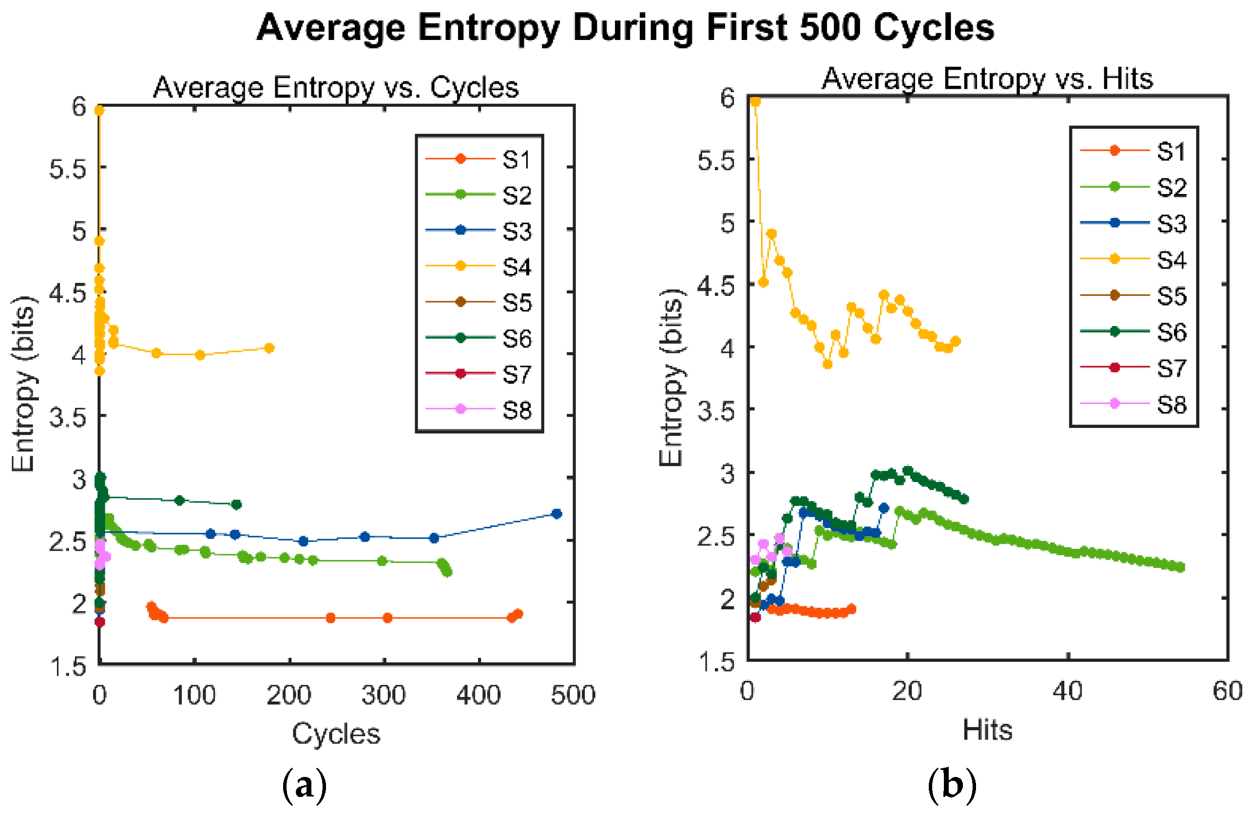
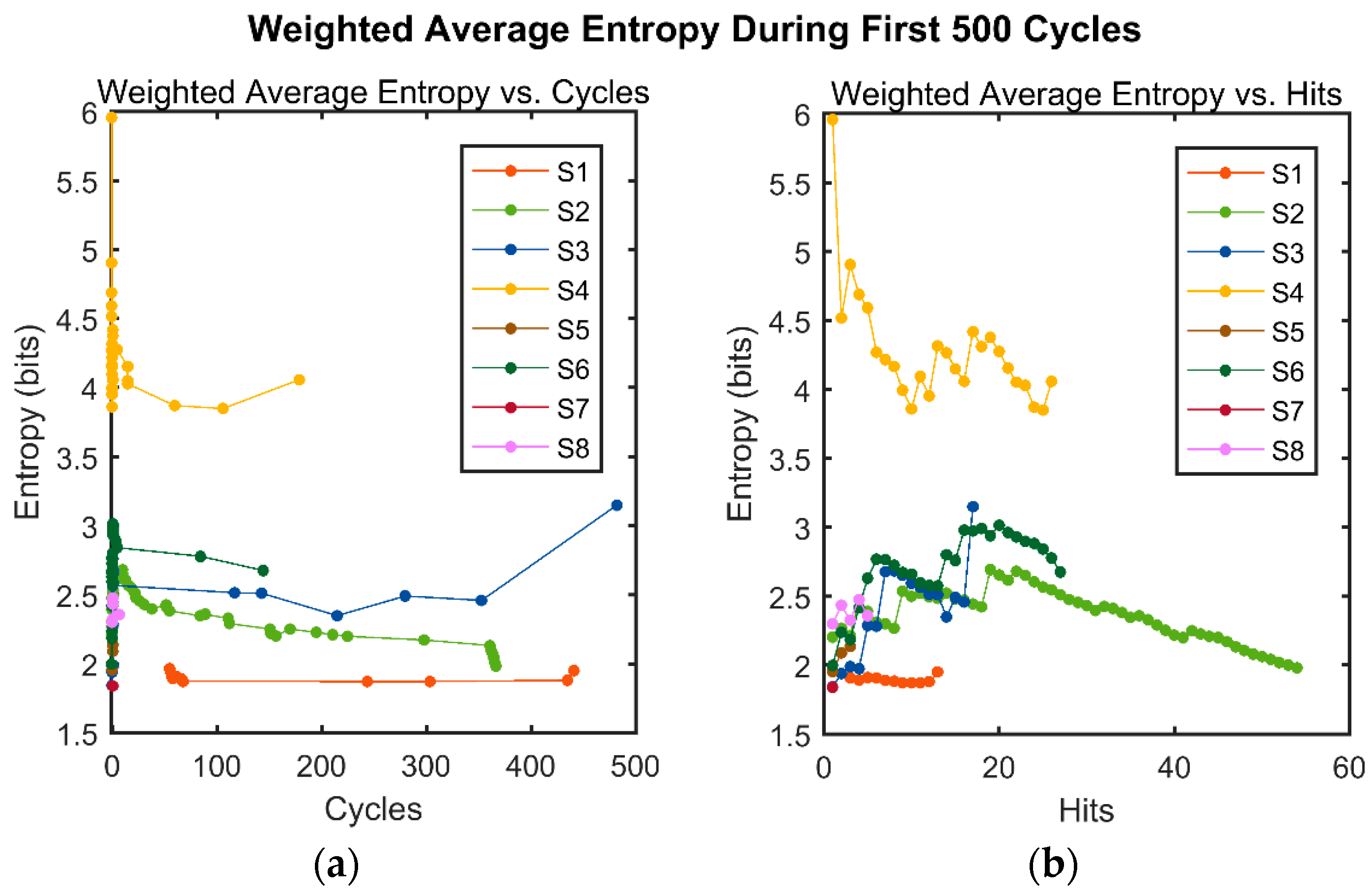
Results validate the hypothesized entropy trends. The average and weighted average entropies for over the first 500 fatigue cycles are plotted against cycles in Figure 11a and Figure 12a, respectively. The entropies vary for the first few signals because the voltage distribution is not yet inertial and heavily dependent on these first initial signal distributions. To more clearly see the variation in average and weighted average entropies at the beginning of cyclic fatigue, Figure 11b and Figure 12b show the entropies for the AE signals versus hit count.
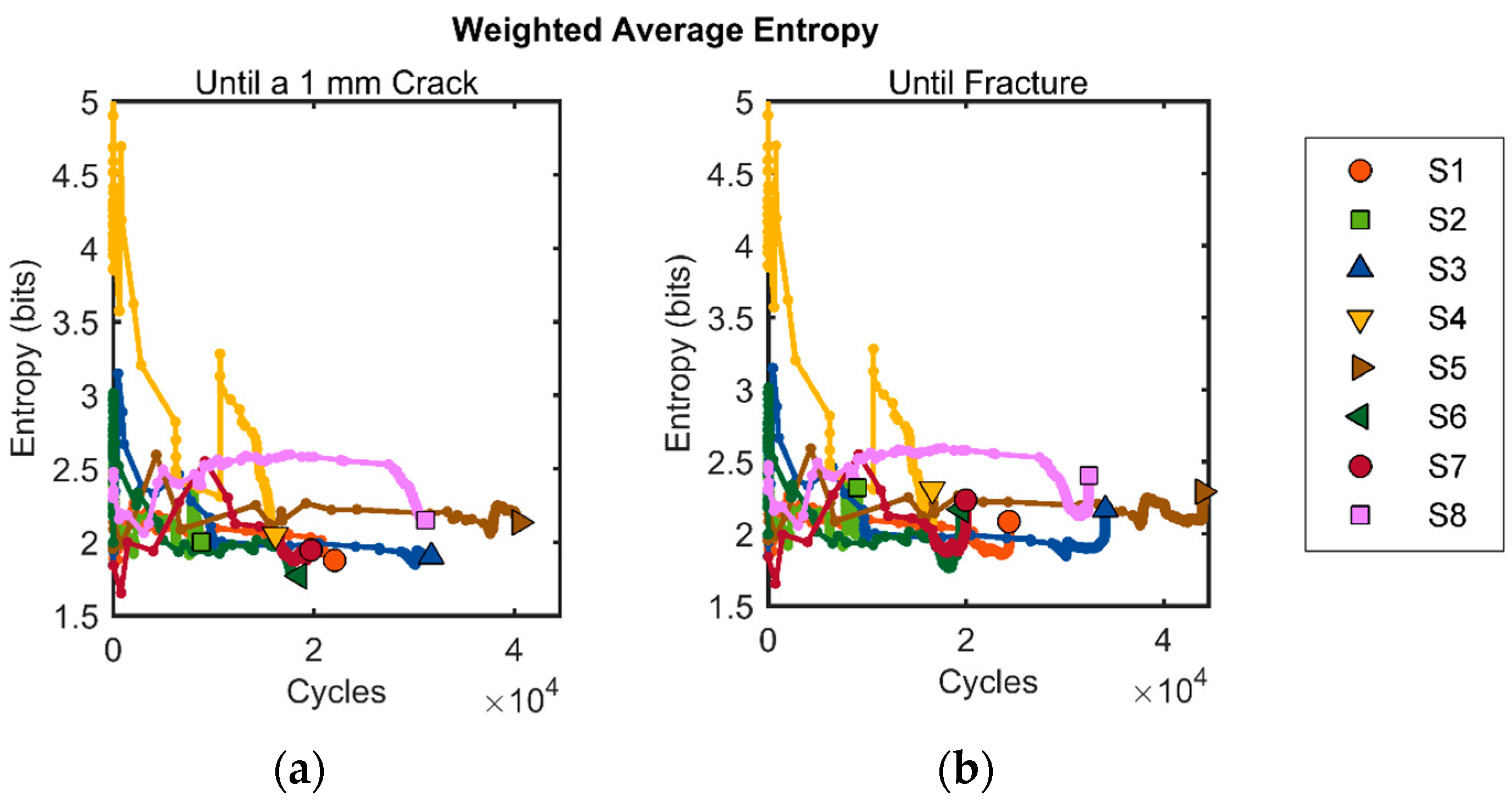
The average and weighted average entropies are then plotted against cycles until both a measured 1-mm crack and fracture occur in Figure 13 and Figure 14. As seen in this figure, sporadic AE signals are received for the majority of life as dislocation pileups and breakaways occur at multiple potential crack initiation sources. After a crack initiates and continues to grow to 1 mm, a common transition length between small and large cracks [46,47,48,49,50,51,52,53], the average and weighted average entropy sharply decreases as shown in Figure 13a and Figure 14a. This finding confirms that entropy decreases after a crack has initiated and that AE signals are more frequent and less disordered. The average and weighted average entropy trends then increase as the crack grows towards fracture as seen in Figure 13b and Figure 14b, again agreeing with the hypothesis. Thus, entropy trends based on accounting for current and previous AE signals may be able to indicate when a crack initiates and grows to a small length, as characterized by a sharp decrease, and when a specimen is near fracture, as described by a sharp increase. The weighted average entropy has the same general trend as average entropy in all graphs but is more irregular during initial fatigue cycles. In the end, there are slight differences between average entropy and weighted average entropy, but both show a noticeable decrease prior to a 1-mm crack followed by an increase as the specimens fracture. Thus, the average or weighted average entropy from AE signals may be able to clearly indicate when an incipient crack is initiating in general metal structures.
5. Conclusions
Cyclic fatigue experiments were performed on Al7075-T6 to investigate potential damage indicators from AE signals. Rather than accepting AE summary statistics such as counts and energy as fully informative damage measures, information entropy was calculated based on the raw voltage data from each recorded AE signal. Three different methods of estimating the information content and the disorder from AE signals were proposed. After developing methods to reduce AE noise, several conclusions were made regarding estimating damage with novel information entropy measures of AE signals. Results support that the proposed instantaneous entropy is a more sensitive statistic and may better correlate to fatigue damage than the AE counts and energy, while the proposed average and weighted average entropy methods provide unique damage trends that could differentiate between small and large cracks. These conclusions are drawn based on coupon-scale fatigue experiments with one high-strength aluminum alloy and therefore the effectiveness of monitoring information entropy metrics over traditional AE summary statistics would need to be verified for other test conditions and materials for the purpose of the model generalization. Even still, when AE is used as an NDE technique to assess fatigue damage and supplement remaining useful life models for aircraft, the information entropy of the signals should be considered to be an important damage metric in addition to the traditionally used signal features.
We have repeated the experiments eight times and the trend of evolution of the information entropy is relatively similar for test of different conditions. Considering the inherent scatter in the results of fatigue test we expect to have relatively similar trends if the tests are repeated.
Supplementary Materials
Supplementary materials are available online at https://www.mdpi.com/2076-3417/7/6/562/s1.
Acknowledgments
This research was supported by the Office of Naval Research under grant number #N00014140453. The authors are grateful for their support.
Author Contributions
Christine M. Sauerbrunn, Huisung Yun, and Ali Kahirdeh conceived and designed the experiments; Christine M. Sauerbrunn and Huisung Yun performed the experiments; Christine M. Sauerbrunn analyzed the data and wrote the manuscript; Huisung Yun, Ali Kahirdeh, and Mohammad Modarres revised the manuscript, and Mohammad Modarres supervised the research.
Conflicts of Interest
The authors declare no conflict of interest. The founding sponsors had no role in the design of the study; in the collection, analyses, or interpretation of data; in the writing of the manuscript, and in the decision to publish the results.
References
- Iyyer, N.; Sarkar, S.; Merrill, R.; Phan, N. Aircraft life management using crack initiation and crack growth models-P-3C Aircraft experience. Int. J. Fatigue 2007, 29, 1584–1607. [Google Scholar] [CrossRef]
- Hoffman, M.E.; Hoffman, P.C. Corrosion and fatigue research—Structural issues and relevance to naval aviation. Int. J. Fatigue 2001, 23, S1–S10. [Google Scholar] [CrossRef]
- Hellier, C.J. Acoustic emission testing. In Handbook of Nondestructive Evaluation; McGraw-Hill: New York, NY, USA, 2001; pp. 10.1–10.39. [Google Scholar]
- Morton, T.M.; Harrington, R.M.; Bjelectich, J.G. Acoustic emissions of fatigue crack growth. Eng. Fract. Mech. 1973, 5, 691–697. [Google Scholar] [CrossRef]
- Bassim, M.N.; Lawrence, S.S.; Liu, C.D. Detection of the onset of fatigue crack growth in rail steels using acoustic emission. Eng. Fract. Mech. 1994, 47, 207–214. [Google Scholar] [CrossRef]
- Berkovits, A.; Fang, D. Study of fatigue crack characteristics by acoustic emission. Eng. Fract. Mech. 1995, 51, 401–416. [Google Scholar] [CrossRef]
- Roberts, T.M.; Talebzadeh, M. Fatigue life prediction based on crack propagation and acoustic emission count rates. J. Constr. Steel Res. 2003, 59, 679–694. [Google Scholar] [CrossRef]
- Roberts, T.M.; Talebzadeh, M. Acoustic emission monitoring of fatigue crack propagation. J. Constr. Steel Res. 2003, 59, 695–712. [Google Scholar] [CrossRef]
- Chang, H.; Han, E.; Wang, J.Q.; Ke, W. Acoustic emission study of corrosion fatigue crack propagation mechanism for LY12CZ and 7075-T6 aluminum alloys. J. Mater. Sci. 2005, 40, 5669–5674. [Google Scholar] [CrossRef]
- Rabiei, M. A Bayesian Framework for Structural Health Management Using Acoustic Emission Monitoring and Periodic Inspections. Ph.D. Dissertation, University of Maryland, College Park, MD, USA, 2011. [Google Scholar]
- Han, A.; Luo, H.; Zhang, Y.; Cao, J. Effects of micro-structure on fatigue crack propagation and acoustic emission behaviors in a micro-alloyed steel. Mater. Sci. Eng. A 2013, 559, 534–542. [Google Scholar] [CrossRef]
- Keshtgar, A. Acoustic Emission-Based Structural Health Management and Prognostics Subject to Small Fatigue Cracks. Ph.D. Dissertation, University of Maryland, College Park, MD, USA, 2013. [Google Scholar]
- Sauerbrunn, C.; Modarres, M. Effects of material variation on acoustic emissions-based, large-crack growth model. In Proceedings of the 2016 25th ASNT Research Symposium, New Orleans, LA, USA, 11–14 April 2016; pp. 105–109. [Google Scholar]
- Vanniamparambil, P.A.; Bartoli, I.; Hazeli, K.; Cuadra, J.; Schwartz, E.; Saralaya, R.; Kontsos, A. An integrated structural health monitoring approach for crack growth monitoring. J. Intell. Mater. Syst. Struct. 2012, 23, 1563–1573. [Google Scholar] [CrossRef]
- Vanniamparambil, P.A.; Guclu, U.; Kontsos, A. Identification of crack initiation in aluminum alloys using acoustic emission. Exp. Mech. 2015, 55, 1–14. [Google Scholar] [CrossRef]
- Aggelis, D.G.; Kordatos, E.Z.; Matikas, T.E. Monitoring of metal fatigue damage using acoustic emission and thermography. J. Acoust. Emiss. 2011, 29, 113–122. [Google Scholar]
- Kordatos, E.Z.; Aggelis, D.G.; Matikas, T.E. Monitoring mechanical damage in structural materials using complimentary NDE techniques based on thermography and acoustic emission. Compos. B Eng. 2012, 43, 2676–2686. [Google Scholar] [CrossRef]
- James, D.; Carpenter, S. Relationship between acoustic emission and dislocation kinetics in crystalline solids. J. Appl. Phys. 1971, 42, 4685–4697. [Google Scholar] [CrossRef]
- Trochidis, A.; Polyzos, B. Dislocation annihilation and acoustic emission during plastic deformation of crystals. J. Mech. Phys. Solids 1994, 42, 1933–1944. [Google Scholar] [CrossRef]
- Polyzos, B.; Trochidis, A. Dislocation dynamics and acoustic emission during plastic deformation of crystals. Wave Motion 1995, 21, 343–355. [Google Scholar] [CrossRef]
- Polyzos, B.; Douka, E.; Trochidis, A. Acoustic emission induced by dislocation annihilation during plastic deformation of crystals. J. Appl. Phys. 2001, 89, 2124–2129. [Google Scholar] [CrossRef]
- Rahman, Z.; Ohba, H.; Yoshioka, T.; Yamamoto, T. Incipient damage detection and its propagation monitoring of rolling contact fatigue by acoustic emission. Tribol. Int. 2009, 42, 807–815. [Google Scholar] [CrossRef]
- Elforjani, M.; Mba, D. Detecting natural crack initiation and crack in slow speed shafts with the acoustic emission technology. Eng. Fail. Anal. 2009, 16, 2121–2129. [Google Scholar] [CrossRef]
- Lugo, M.; Jordon, J.B.; Horstemeyer, M.F.; Tschopp, M.A.; Harris, J.; Gokhale, A.M. Quantification of damage evolution in a 7075 aluminum alloy using an acoustic emission technique. Mater. Sci. Eng. A Struct. 2011, 528, 6708–6714. [Google Scholar] [CrossRef]
- Chaswal, V.; Sasikala, G.; Ray, S.K.; Mannan, S.L.; Raj, B. Fatigue crack growth mechanism in aged 9Cro-1Mo steel: Threshold and Paris regimes. Mater. Sci. Eng. A Struct. 2005, 395, 251–264. [Google Scholar] [CrossRef]
- Han, Z.; Luo, H.; Sun, C.; Li, J.; Papaelias, M.; Davis, C. Acoustic emission study of fatigue crack propagation in extruded AZ31 magnesium alloy. Mater. Sci. Eng. A Struct. 2014, 597, 270–278. [Google Scholar] [CrossRef]
- Čapek, J.; Máthis, K.; Clausen, B.; Stráská, J.; Beran, P.; Lukáš, P. Study of the loading mode dependence of the twinning in random textured cast magnesium by acoustic emission and neutron diffraction methods. Mater. Sci. Eng. A Struct. 2014, 602, 25–32. [Google Scholar] [CrossRef]
- Mazal, P.; Vlasic, F.; Koula, V. Use of acoustic emission method for identification of fatigue micro-cracks creation. Procedia Eng. 2015, 133, 379–388. [Google Scholar] [CrossRef]
- Gager, D.; Foote, P.; Irving, P.E. Effects of loading and sample geometry on acoustic emission generation during fatigue crack growth: Implications for structural health monitoring. Int. J. Fatigue 2015, 81, 117–127. [Google Scholar] [CrossRef]
- Shiotani, T.; Aggelis, D.G. Wave propagation in cementitious material containing artificial distributed damage. Mater. Struct. 2009, 42, 377–384. [Google Scholar] [CrossRef]
- Sauerbrunn, C. Evaluating Information Entropy from Acoustic Emission Waveforms As a Fatigue Damage Metric for Al7075-T6. Master’s Thesis, University of Maryland, College Park, MD, USA, 2016. [Google Scholar]
- Unnthorsson, R.; Runarsson, T.; Jonsson, M. AE entropy for the condition monitoring of CFRP subjected to cyclic failure. J. Acoust. Emiss. 2008, 26, 262–269. [Google Scholar]
- Qi, G.; Fan, M.; Lewis, G. An innovative multi-component variate that reveals hierarchy and evolution of structural damage in a solid: Application to acrylic bone cement. J. Mater. Sci. Mater. Med. 2012, 23, 217–228. [Google Scholar] [CrossRef] [PubMed]
- Ramasso, E.; Placet, V.; Boubakar, L. Unsupervised consensus clustering of acoustic emission time-series for robust damage sequence estimation in composites. IEEE Trans. Instrum. Meas. Soc. 2015, 64, 3297–3307. [Google Scholar] [CrossRef]
- Amiri, M.; Modarres, M. AE entropy for detection of fatigue crack initiation and growth. In Proceedings of the 2015 IEEE Conference on Prognostics and Health Management, Austin, TX, USA, 22–25 June 2015; pp. 1–8. [Google Scholar]
- Kahirdeh, A.; Sauerbrunn, C.; Modarres, M. Acoustic emission entropy as a measure of damage in materials. In Proceedings of the 35th MAXENT Conference, Postdam, NY, USA, 19–24 July 2015. [Google Scholar]
- Shannon, C.E. A mathematical theory of communication. Bell Syst. Tech. J. 1948, 27, 379–423, 623–656. [Google Scholar] [CrossRef]
- MacKay, D.J.C. Information Theory, Inference, and Learning Algorithms; Cambridge University Press: Cambridge, UK, 2003. [Google Scholar]
- Standard Practice for Conducting Force Controlled Constant Amplitude Axial Fatigue Tests for Metallic Materials; ASTM E466-07; ASTM International: West Conshohocken, PA, USA, 2007.
- Pilkey, W.D. Peterson’s Stress Concentration Factors; John Wiley & Sons, Inc.: New York, NY, USA, 1997. [Google Scholar]
- Standard Practice for Determining the Reproducibility of Acoustic Emission Sensor Response; ASTM E976-15; ASTM International: West Conshohocken, PA, USA, 2015.
- Miller, R. Acoustic emission: An Application to Fracture Mechanics. Ph.D. Dissertation, Purdue University, West Lafayette, IN, USA, 1979. [Google Scholar]
- Kharrat, M.; Ramasso, E.; Placet, V.; Boubakar, M.L. A signal processing approach for enhanced acoustic emission data analysis in high activity systems: Application to organic matrix composites. Mech. Syst. Signal. Process. 2016, 70–71, 1038–1055. [Google Scholar] [CrossRef]
- Doan, D.D.; Ramasso, E.; Placet, V.; Zhang, S.; Boubakar, L.; Zerhouni, N. An unsupervised pattern recognition approach for AE data originating from fatigue tests on polymer–composite materials. Mech. Syst. Signal. Process. 2015, 64, 465–478. [Google Scholar] [CrossRef]
- Dzenis, Y.A. Cycle-based analysis of damage and failure in advanced composites under fatigue: 1. Experimental observation of damage development within loading cycles. Int. J. Fatigue 2003, 25, 499–510. [Google Scholar] [CrossRef]
- Kachanov, L. On time to rupture in creep conditions. Izviestia Akademii Nauk SSSR Otdelenie Tekhnicheskikh Nauk 1958, 8, 26–31. (In Russian) [Google Scholar]
- Schijve, J. Fatigue of Structures and Materials; Kluwer Academic Publishers: Dordrecht, The Netherlands, 2001. [Google Scholar]
- Wu, X.R.; Newman, J.C.; Zhao, W.; Swain, M.H.; Ding, C.F.; Phillips, E.P. Small crack growth and fatigue life predictions for high-strength aluminum alloys: Part I—Experimental and fracture mechanics analysis. Fatigue Fract. Eng. 1998, 21, 1289–1306. [Google Scholar] [CrossRef]
- Newman, J.C.; Wu, X.R.; Swain, M.H.; Zhao, W.; Phillips, E.P.; Ding, C.F. Small crack growth and fatigue life predictions for high-strength aluminum alloys: Part II—Crack closure and fatigue analyses. Fatigue Fract. Eng. 1999, 23, 59–72. [Google Scholar] [CrossRef]
- Forth, S.C.; Newman, J.C., Jr.; Forman, R.G. On generating fatigue crack growth thresholds. Int. J. Fatigue 2003, 25, 9–15. [Google Scholar] [CrossRef]
- Suresh, S.; Ritchie, R.O. Propagation of short fatigue cracks. Int. Met. Rev. 1984, 29, 445–475. [Google Scholar] [CrossRef]
- Pook, L. Metal Fatigue: What It Is, Why It Matters; Springer: Dordrecht, The Netherlands, 2007. [Google Scholar]
- Xue, Y.; McDowell, D.L.; Horstemeyer, M.F.; Dale, M.H.; Jordon, J.B. Microstructure-based multistage fatigue modeling of aluminum alloy 7075-T651. Eng. Fract. Mech. 2007, 74, 2810–2823. [Google Scholar] [CrossRef]
Figure 1.
Probability mass functions (PMF) of various weighted coins and the associated calculated entropy: (a) PMF of flipping a fair coin and calculated entropy; (b) PMF of a biased coin with probability of flipping tails as 0.70 and calculated entropy; and (c) PMF of a biased coin with probability of flipping tails as 0 and calculated entropy.
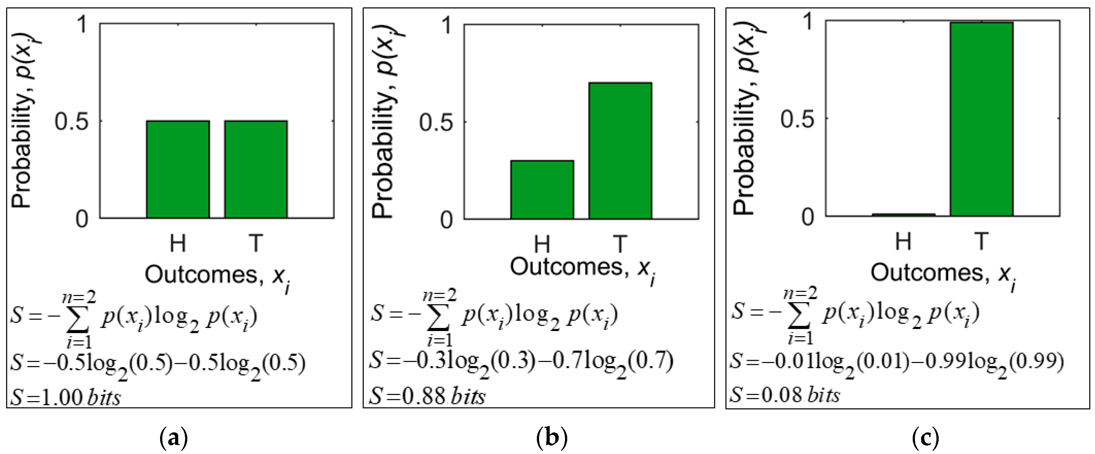
Figure 2.
Waveforms, voltage distributions, and information entropy values for three AE (acoustic emission) signals: (a) Signal A captured during relatively little microstructural change; (b) Signal B captured during a moderate microstructural change; and (c) Signal C captured during a relatively significant microstructural change.
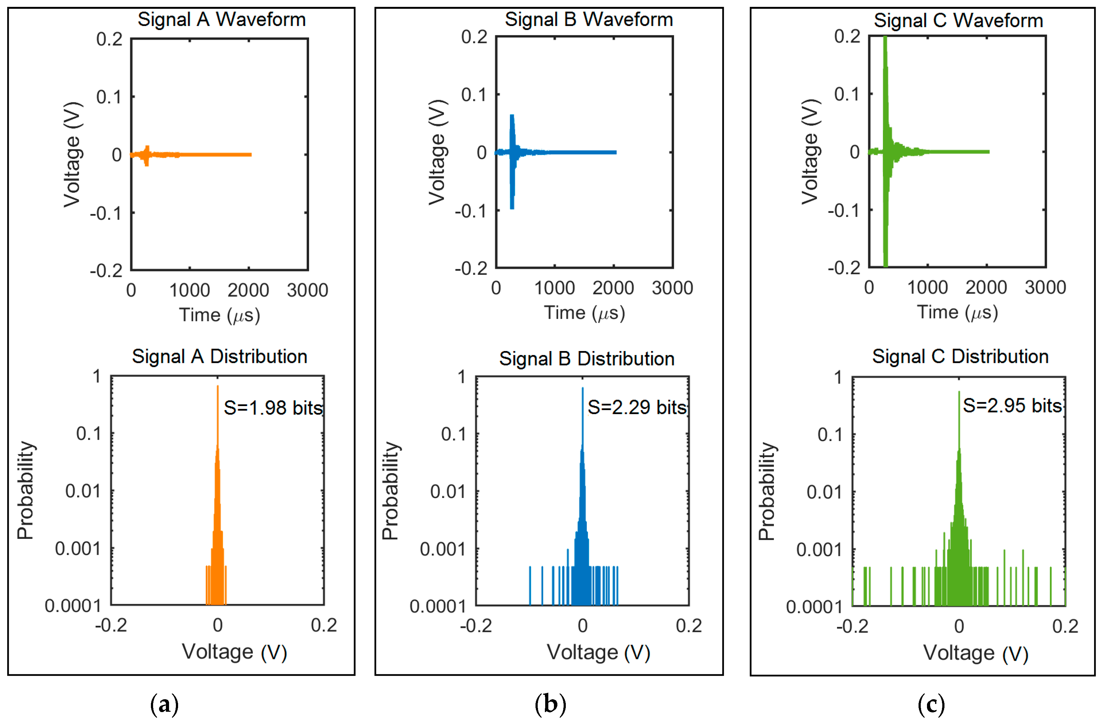
Figure 3.
Representative AE waveforms at various instances during the S2 experiment: (a) two signals measured in the beginning of the S2 test; (b) two signals measured in the instant of crack initiation in the S2 test; and (c) two signals measured at instant of complete fracture of the specimen in S2 test.

Figure 4.
Experimental setup showing the specimen, AE sensors, mechanical damping apparatus and crack growth monitoring system.
Figure 4.
Experimental setup showing the specimen, AE sensors, mechanical damping apparatus and crack growth monitoring system.

Figure 5.
Effect of AE hit length on instantaneous, average, and weighted average entropy showing that the entropy of AE signals with longer hit lengths have lower values than shorter hit lengths while the trends between the entropies are unaffected by the hit length.
Figure 5.
Effect of AE hit length on instantaneous, average, and weighted average entropy showing that the entropy of AE signals with longer hit lengths have lower values than shorter hit lengths while the trends between the entropies are unaffected by the hit length.

Figure 6.
AE signals at their associated loads versus time for three experiments: (a) S8 has no apparent AE noise clusters; (b) S4 has defined clusters that are assumed to be due to noise and can be filtered; (c) another experiment with undefined clusters of noise signals that cannot be filtered with ease; (d) cumulative AE hits over time for S8 with no apparent AE noise clusters; (e) cumulative AE hits over time for S4 with filterable noise; and (f) cumulative AE hits for an experiment with unfilterable noise.
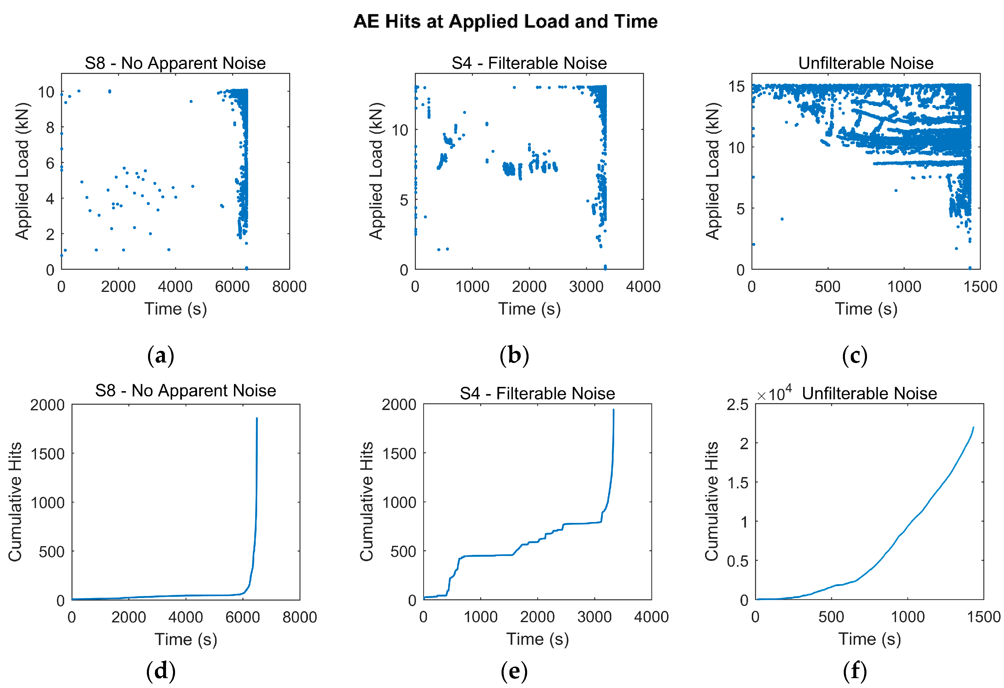
Figure 7.
Cumulative trend for three parameters versus fatigue cycles for specimen 1 (S1) to specimen 8 (S8): (a) cumulative instantaneous entropy; (b) cumulative counts; and (c) cumulative energy.
Figure 7.
Cumulative trend for three parameters versus fatigue cycles for specimen 1 (S1) to specimen 8 (S8): (a) cumulative instantaneous entropy; (b) cumulative counts; and (c) cumulative energy.
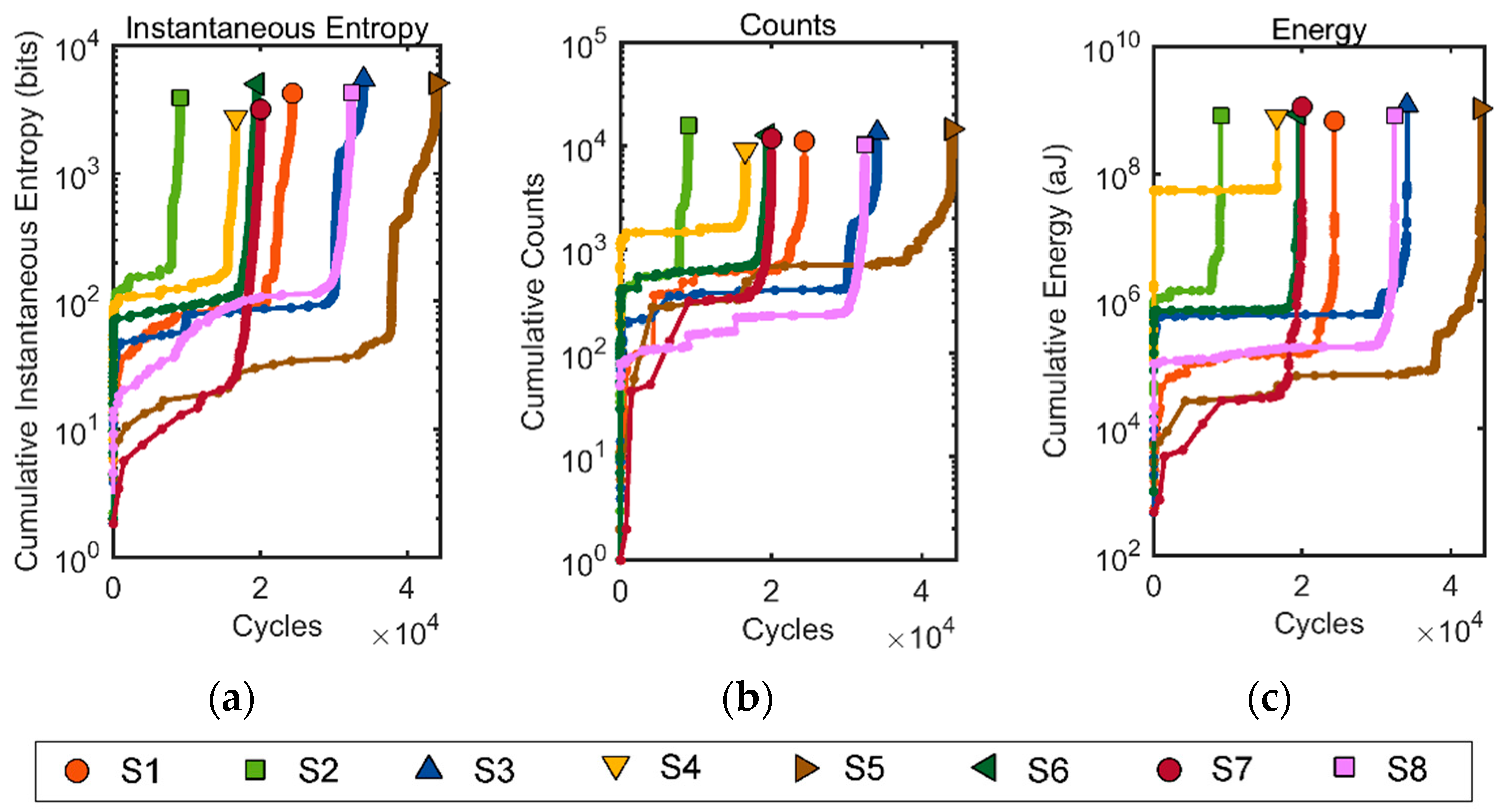
Figure 8.
Modulus degradation damage (MDD) plotted versus cycles until specimen fracture for all experiments (S1 to S8).
Figure 8.
Modulus degradation damage (MDD) plotted versus cycles until specimen fracture for all experiments (S1 to S8).
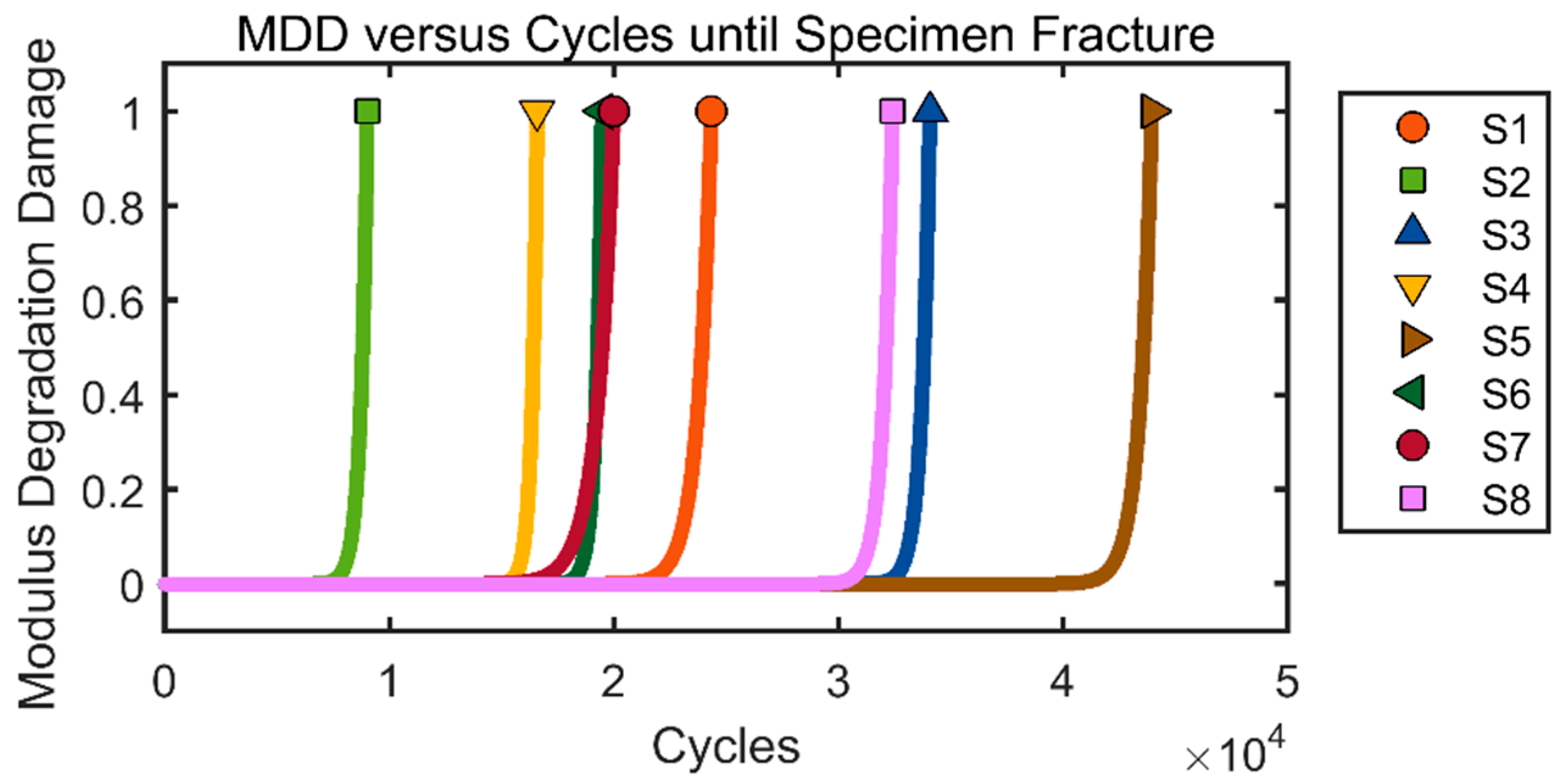
Figure 9.
Normalized cumulative trend for three parameters with respect to measured damage or MDD where a one-to-one relationship is desired: (a) instantaneous entropy; (b) energy; and (c) counts.
Figure 9.
Normalized cumulative trend for three parameters with respect to measured damage or MDD where a one-to-one relationship is desired: (a) instantaneous entropy; (b) energy; and (c) counts.

Figure 10.
Deviation factor for AE counts, energy, and instantaneous entropy for all experiments.
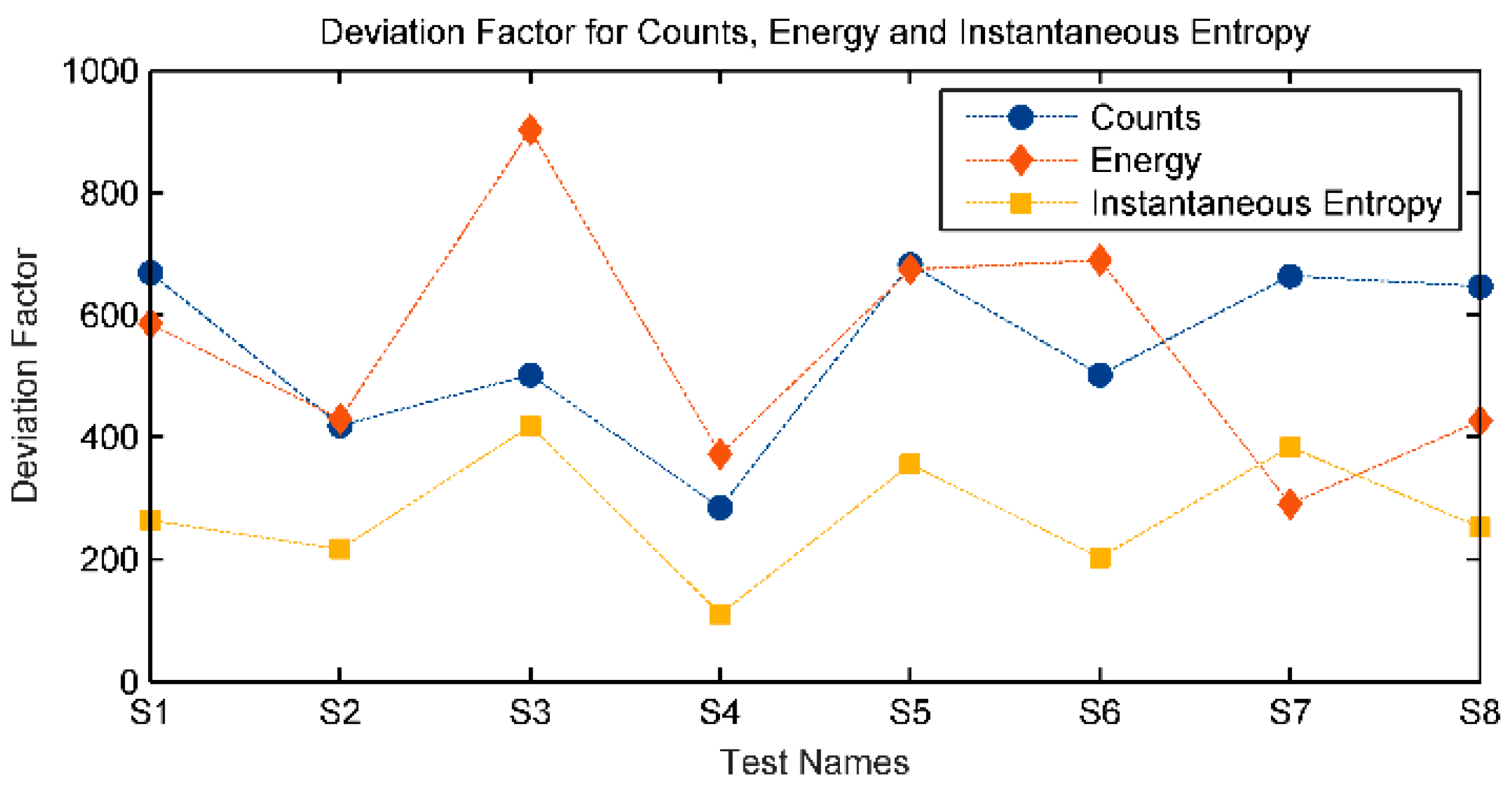
Figure 11.
Average entropy trends versus fatigue cycles and hit count over the first 500 cycles: (a) average entropy versus cycles; and (b) average entropy versus hits.
Figure 11.
Average entropy trends versus fatigue cycles and hit count over the first 500 cycles: (a) average entropy versus cycles; and (b) average entropy versus hits.

Figure 12.
Weighted average entropy trends versus fatigue cycles and hit count over the first 500 cycles: (a) weighted average entropy versus cycles; and (b) weighted average entropy versus hits.
Figure 12.
Weighted average entropy trends versus fatigue cycles and hit count over the first 500 cycles: (a) weighted average entropy versus cycles; and (b) weighted average entropy versus hits.

Figure 13.
Average entropy trends versus fatigue cycles through two damage levels: (a) average entropy until a 1-mm crack; and (b) average entropy until fracture.
Figure 13.
Average entropy trends versus fatigue cycles through two damage levels: (a) average entropy until a 1-mm crack; and (b) average entropy until fracture.
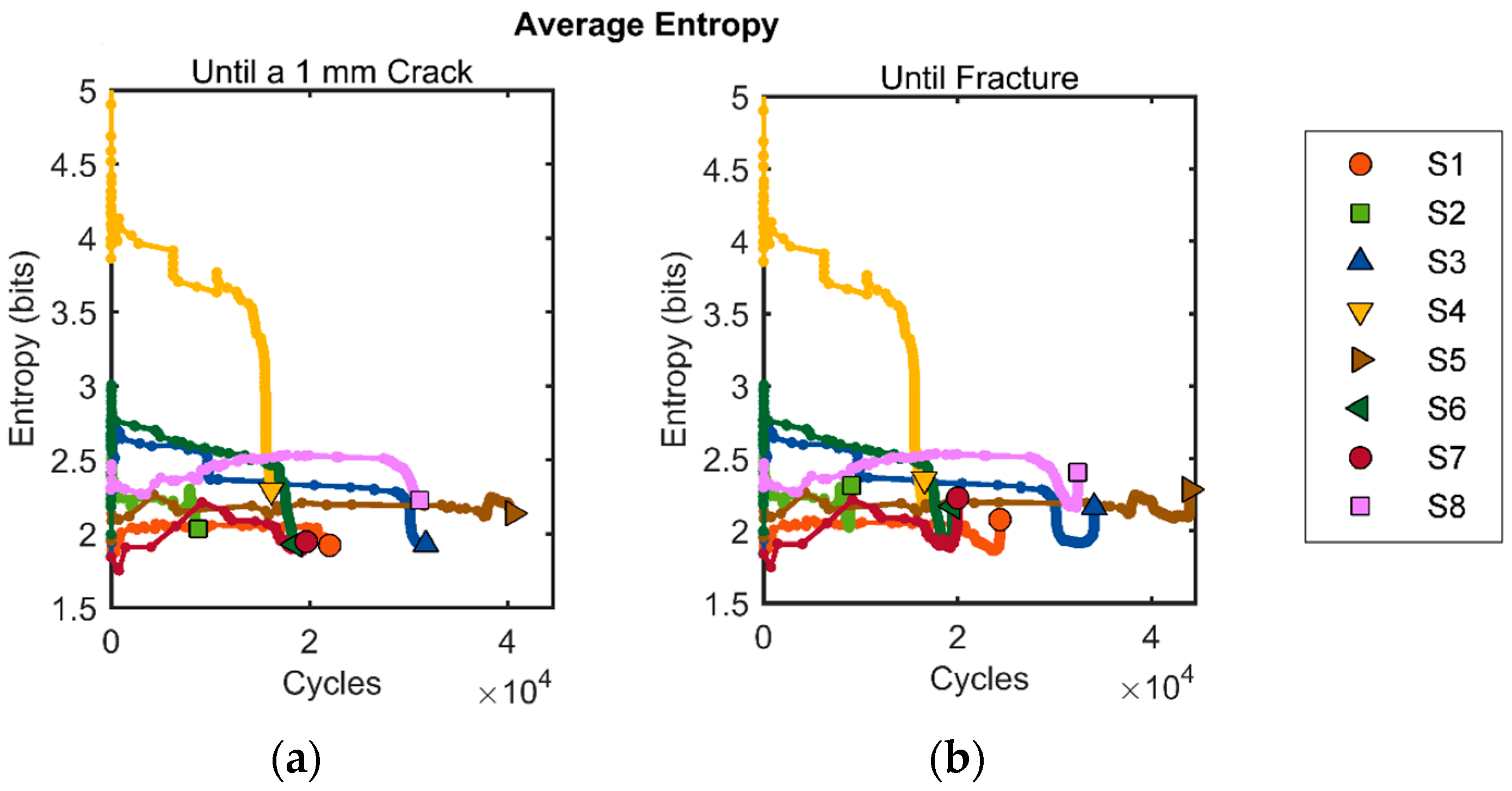
Figure 14.
Weighted average entropy trends versus fatigue cycles through two damage levels: (a) weighted average entropy until a 1-mm crack; and (b) weighted average entropy until fracture.
Figure 14.
Weighted average entropy trends versus fatigue cycles through two damage levels: (a) weighted average entropy until a 1-mm crack; and (b) weighted average entropy until fracture.

Table 1.
Composition and mechanical properties of Al7075-T6.
| Element | Al | Zn | Mg | Cu | Cr | Fe | Mn | Si | Ti | V | Zr | Other |
|---|---|---|---|---|---|---|---|---|---|---|---|---|
| Composition (wt %) | 89.7 | 5.7 | 2.6 | 1.4 | 0.20 | 0.15 | 0.08 | 0.06 | 0.02 | 0.01 | 0.01 | 0.05 |
| Material Property | Ultimate Strength (MPa) | Yield Strength (MPa) | Elastic Modulus (GPa) | |||||||||
| Property Value | 587 | 538 | 67.8 | |||||||||
Table 2.
AE (acoustic emission) software settings.
| Parameter | Value |
|---|---|
| Peak definition time (PDT) | 300 µs |
| Hit definition time (HDT) | 600 µs |
| Hit lockout time (HLT) | 1000 µs |
| Sampling rate | 1 MSPS |
| Pre-trigger length | 256 µs |
| Hit length | 2048 µs |
| Band pass filter | 1 kHz–3 MHz |
Table 3.
Statistics for final cumulative values of instantaneous entropy, counts, and energy.
| Cumulative AE Parameter | Mean (µ) | Standard Deviation (σ) | Coefficient of Variation (CV, %) |
|---|---|---|---|
| Instantaneous entropy | 4221.6 bits | 945.2 bits | 22.4 |
| Counts | 12,360 | 2245 | 18.2 |
| Energy | 9.21 × 10⁸ aJ | 1.87 × 10⁸ aJ | 20.2 |
© 2017 by the authors. Licensee MDPI, Basel, Switzerland. This article is an open access article distributed under the terms and conditions of the Creative Commons Attribution (CC BY) license (http://creativecommons.org/licenses/by/4.0/).
Share and Cite
MDPI and ACS Style
Sauerbrunn, C.M.; Kahirdeh, A.; Yun, H.; Modarres, M. Damage Assessment Using Information Entropy of Individual Acoustic Emission Waveforms during Cyclic Fatigue Loading. Appl. Sci. 2017, 7, 562. https://doi.org/10.3390/app7060562
AMA Style
Sauerbrunn CM, Kahirdeh A, Yun H, Modarres M. Damage Assessment Using Information Entropy of Individual Acoustic Emission Waveforms during Cyclic Fatigue Loading. Applied Sciences. 2017; 7(6):562. https://doi.org/10.3390/app7060562
Chicago/Turabian StyleSauerbrunn, Christine M., Ali Kahirdeh, Huisung Yun, and Mohammad Modarres. 2017. "Damage Assessment Using Information Entropy of Individual Acoustic Emission Waveforms during Cyclic Fatigue Loading" Applied Sciences 7, no. 6: 562. https://doi.org/10.3390/app7060562
Note that from the first issue of 2016, this journal uses article numbers instead of page numbers. See further details here.