
Computational Fluid Dynamics Analysis of Cold Plasma Plume Mixing with Blood Using Level Set Method Coupled with Heat Transfer

Department of Physics and Materials Science, City University of Hong Kong, Hong Kong, China
*
Author to whom correspondence should be addressed.
Appl. Sci. 2017, 7(6), 578; https://doi.org/10.3390/app7060578
Submission received: 27 April 2017
/
Revised: 25 May 2017
/
Accepted: 31 May 2017
/
Published: 3 June 2017
(This article belongs to the Special Issue Advances in Thermal System Analysis and Optimization)
Abstract
:Cold plasmas were proposed for treatment of leukemia. In the present work, conceptual designs of mixing chambers that increased the contact between the two fluids (plasma and blood) through addition of obstacles within rectangular-block-shaped chambers were proposed and the dynamic mixing between the plasma and blood were studied using the level set method coupled with heat transfer. Enhancement of mixing between blood and plasma in the presence of obstacles was demonstrated. Continuous tracking of fluid mixing with determination of temperature distributions was enabled by the present model, which would be a useful tool for future development of cold plasma devices for treatment of blood-related diseases such as leukemia.
1. Introduction
A novel technique and a conceptual design of a mixing chamber were presented in the current study that could be used in future development of effective cold plasma devices for treatment of blood related syndromes such as leukemia.
Plasma medicine research has been progressing very rapidly in recent years [1,2,3]. Cold atmospheric plasmas have shown significant potentials in various biomedical applications such as wound healing [4,5], tooth bleaching [6], cancer therapy [7,8,9] and sterilization of infected tissues [10]. In recent years, cold atmospheric plasmas were explored for inactivating different microorganisms. They were found effective in decontaminating chicken skin and muscle inoculated with Listeria innocua [11]. Inhomogeneous inhabitation zones were generated in microcolonies by high flow rates of helium [12]. Furthermore, cold plasmas were found to show microbicidal and sporicidal effects but at the same time low toxicity for mammalian tissues [13]. Cold plasmas were also employed to treat the surface of polymers, including polyethylene with an ultra-high molecular weight used as joint replacements, and were additionally found able to enhance adhesion between the joint-replacement material and bone [14] as well as the wear performance of the polymer [15].
Therapeutic use of interaction between cold plasma and blood was successfully carried out [16]. Mixing between cold plasma and blood was also explored for treatment of large bleeding areas and for blood coagulation [17,18,19]. In relation, the viability and proliferation of human peripheral blood mononuclear cells upon exposures to atmospheric pressure argon plasma jets were studied, and significant cell damages for short plasma exposures were not observed [20]. The effect of cold plasma jet on wound healing was also comprehensively studied, and no significant effects from cold-plasma treatment were found on white blood cells, red blood cells, aspartate aminotransferase, alanine aminotransferase, blood urea nitrogen, or creatine contents [21]. More recently, possible use of non-thermal gas plasma as an alternative treatment scheme against leukemia was explored for the first time by Barekzi et al., and it was found that the therapeutic effect of plasma on leukemia cells was not immediate (it has a delayed effect) and the increase in leukemia cell killing was achieved by increasing the contact time between the cold plasma plume and the cancerous human T-cell leukemia cells [22]. Furthermore, selective natural mechanisms of blood coagulation were triggered when blood samples were exposed to plasmas generated by non-thermal atmospheric pressure dielectric barrier (DBD) discharge at room temperature and pressure [23]. Moreover, the difficulty in directly treating blood with cold plasmas due to the coagulation was noted by Chen et al., so injection of cold plasma solution into the blood around the tumor was explored by the authors, involving three different carrier gases, i.e., helium (He), argon (Ar) and nitrogen (N2) [24]. It was pointed out by Shimizu et al. that cold plasma discharges had very low gas temperatures due to weak ionization rate for electron collisions and reactions [25]. The concentration of reactive species in the plasmas could be altered by the applied voltage [15]. In order to enhance the plasma chemistry while maintaining a low plasma temperature, very short voltage pulses (in the range from nanoseconds to microseconds) could be applied [22]. Moreover, the chemical reactions in plasmas were affected by the vibrational temperature, since the molecules were dissociated through their vibrational and electronic excitations [26]. On the other hand, the plasma characteristics were also affected by the plasma frequency since the very short lifetime of the charged particles could be comparable or even shorter than the applied pulse width. For example, in a previous study, the plasma frequency was set to be at 5 kHz and the pulse width was set at 0.50 μs [22]. Moreover, the fractions of plasma constituents were found to be small and therefore no significant additional heat was produced as a result of reactions in the discharge, so the bulk temperature of the carrier gas would be the dominating factor in determining the plume temperature [27,28,29].
From the previous studies, the two main challenges regarding the treatment of blood related diseases such leukemia are: (1) the contact between the plasma and the blood needs to be maximized; and (2) at the same time the blood coagulation needs to be minimized so that maximum contact could be achieved. In order to maximize the efficiency and effectiveness of these treatments and at the same time overcome the mentioned challenges, the contact/mixing between the plasma plume and blood needs to be enhanced dynamically; this requires a versatile multiphysics model for thermofluid analysis of the cold plasmas which has been somehow overlooked in most previous investigations. A parameterized model was set up by Schröder et al. [30] to simulate the species densities generated by a plasma needle and also the heat transfer to a skin layer. However, the model developed by Schröder et al. did not consider the plasma plume and its transfer to the treatment zone. Finite element analyses were also previously employed in simulation of atmospheric pressure plasma needles, without considering thermofluid analyses [31,32].
In the present work, two different conceptual designs of the mixing chamber were studied to accomplish a better mixing and to increase the contact between the blood and plasma plume by modifying the previous multiphysics model based on the level set method coupled with heat transfer [29]. It is remarked here that the present designs (i.e., with and without obstacles) of mixing chambers for blood and plasma only serve to demonstrate the concept of enhanced mixing by addition of obstacles to the flow. To the best of our knowledge, there were no previous designs in the literature. Upon an even mixing between the cold plasma and blood with precise probing of thermofluid parameters, an effective mixing could be achieved despite the relatively higher blood viscosity [24] compared to the plasma. Furthermore, information would be provided by dynamic tracking of both fluids in the mixing chambers on the underlying mechanism of mixing between the blood and cold plasma plume.
2. Materials and Methods
2.1. Mathematical Models
The level set function coupled with heat transfer, continuity and Navier–Stokes equations were discretized and solved numerically using the finite element method (FEM). The blood and cold plasma plume in the mixing chamber domain were tracked with the level set method using the level set variable (). The standard heat equation was used to model the heat transfer between the two fluids within the mixing chamber. The present theoretical model consisted of two main parts: (1) fluid dynamics with level set interface module; and (2) heat transfer module, which were coupled to each other. The results were obtained using parallel computing.
In the present work, the level set method was used to capture the mixing and evolution of blood in cold plasma in two different mixing chamber designs in three-dimensional coordinate system, which was a continuation of our previous work in which the level set method was used to simulate cold plasma plume propagation in a cell buffer medium [29]. The level set method has been extensively used in simulation of two-phase fluid systems in which a liquid–gas interface is present [33,34,35,36]. Applications of 3D computational fluid dynamics (CFD) simulations were aimed at providing realistic information and data [37] and at demonstrating the versatility and capability of the model over simplified models such as 2D axisymmetric models for cylindrical chambers. The present model was based on our previously developed theory and here it was modified for the present two-phase fluid systems [29]. The plasma carrier gas was assumed to be helium (He) and its evolution in the mixing chamber that got filled with the injected blood was explained using the level set function as
where was the level set function, ε was the interface thickness equivalent to the largest mesh element size mainly to allow a better interface reconstruction between the two fluids [29] and its value here was 4 × 10⁻⁴ m. Oscillations in the level set function were reduced by the parameter γ to keep the interface thickness constant to achieve better numerical stability, and γ was set to be the largest initial velocity in the system to effectively decrease the oscillations in the level set function [29], which in this case was 0.1.
The continuity equation defined in the mixing chamber involving blood and cold plasma is given by
The Navier–Stokes momentum equation is given by
where ρ is density, P is pressure, u is the velocity of the flow, F is given by F = ρg + Fst + Fvf, ρg is the body force, Fst is the surface tension and Fvf is the volume force. Furthermore, the heat transfer in the mixing chamber is explained using the heat equation, with the use of the thermophysical properties of blood and plasma carrier gas:
where Cp is the specific heat capacity, ρ represents the density, k is the thermal conductivity and Q represents any external source of heat energy, which can be evaluated as heat energy generated per unit volume. In the present work, instead of defining an external heat source Q, the initial temperatures of the fluids at the inlet boundaries of the nozzles were chosen. Furthermore, Equation (4) can be written as
2.2. Solver
Since the domain Ω was divided into finite elements connected at the nodes, the global equations for Ω were assembled from equations for the elements in Ω. The shape function for temperature interpolation inside the finite elements would be
Differentiation of the temperature interpolation equation led to temperature gradients as shown in Equation (7)
where {T} represented the vector temperature at the nodes, [N] was the matrix of shape functions and [B] was the matrix for temperature-gradient interpolation. Applying the Galerkin method, the heat transfer equation would became
After applying the divergence theorem and discretization, the obtained linear system was solved using the Generalized Minimal Residual Method (GMRES) iterative solver [40]. For a linear system of equations Ax = b, the general idea behind the GMRES solver with left preconditioning for Krylov subspace with initial guess of v to the solution would have the form
The approximate solution x was chosen in a way to minimize the residual that had the form of r = Ax − b. The algorithm of the left-preconditioned GMRES method is described in Appendix A. Due to the complexities involved in the multi-physics system, the present model was solved in parallel using the Message Passing Interface (MPI) which allowed numerical simulations to be performed on multiple compute units. In the present work, the MPICH2 package was employed for parallel computing [41]. The source of the “heat” used to regulate the temperature of the injected blood and plasma was characterized by constant temperatures at the inlet boundaries, i.e., Tfluid = T0, where T0 was 310 and 303 K for blood and plasma, respectively.
2.3. Test Case Geometry
Moreover, the proposed conceptual design of the chambers contained three inlet nozzles, two of which used to inject plasmas into the chamber while the third used to inject blood simultaneously. Initially, the chamber was assumed to be filled with cold plasma that enabled the interface initialization for the level set variable (). In addition, movement of blood and plasma into the chamber and their subsequent mixing until their final discharge from the outlet nozzle were continuously tracked by the level set method. The geometries of the mixing chambers with and without obstacles are shown in Figure 1a,b, respectively.
The dimensions of blood and cold plasma inlet nozzles were (5 × 1 × 1) × 10−6 m3 and (1 × 1 × 1) × 10−6 m3, respectively, while those of the outlet nozzle were (5 × 2 × 1)×10−6 m3. The total length of the mixing chamber was 0.1 m and the width was 5 × 10⁻² m. The dimensions of the obstacles were (1 × 2 × 1) × 10−6 m3. The blood flowrates in portal vein and cardiac output were 1.92 and 9.33 m3 s−1, respectively, so the average blood flowrate was 5.63 m3 s−1 [42]. For the two mixing chamber configurations shown in Figure 1a,b, the blood inlet velocity was chosen as 0.1 m s−1 to generate a matching blood flowrate. It is remarked that the velocity of the plasma carrier gas could vary [43], and the plasma inlet velocity from the (1 × 1) × 10−4 m2 inlet nozzle was also set as 0.1 m s−1 here for simplicity. The fluid flow in the present work was in the laminar regime, since the largest Reynolds number (Re = ρVD/μ) was ~530 which was far below ~4000 for the turbulent regime. Moreover, the material properties of plasma carrier gas and blood used as inputs to the present model are summarized in Table 1.
2.4. Boundary Conditions
In order to solve the system of partial differential equations (PDEs), the boundary conditions for fluid dynamics and heat transfer module would be needed. The no-slip boundary condition (u = 0, where u is the velocity field) was assigned to the inner boundary of the device, which indicated the presence of adhesion between fluids and the solid wall. In the heat transfer module, the surrounding wall was assumed as thermally insulated (−n·q = 0, where q is the heat flux). The inlet nozzles for injection of cold plasma had the form uleft = ux+ and uright = ux− for the left and right nozzle as shown in Figure 1a,b, respectively. The values of ux+ and ux− were set to be 0.1 ms−1 for the two different cases used to study the mixing phenomena and the level set variable at the inlets was = 0; this indicated the presence of plasma. Considering the blood inlet nozzle ( = 1 at the inlet nozzle), the inlet velocity of the blood uupward = uy+ was set as 0.1 ms−1, so that mixing chamber filling and steady-state could be fully obtained during the simulation time of 10.0 s. In addition, linear discretization was employed using an average element quality of ~2 × 10⁻⁴ m. Numerical convergence was verified by considering simulations with different grid resolutions and no inconsistencies were observed in numerical convergence and the final results. The mesh figures for the two configurations of the mixing chamber are shown in Figure 2.
2.5. Grid Sensitivity Analysis (GSA)
Grid sensitivity analysis (GSA) was performed for the mixing chambers with obstacles, mainly to assess the reliability and accuracy of the present model. The two main parameters chosen for GSA were the blood volume fraction exiting the outlet boundary of the mixing chamber (which demonstrated the reliability and accuracy of fluid dynamics with level set interface module) and the temperature of the outlet nozzle (which demonstrated the reliability and accuracy of the heat transfer module). Three different grid sizes were considered using the concept of grid refinement factor (r) defined as
where hcoarse was the mesh or grid size before refinement while hfine was the mesh or grid size after refinement. In practice, r should be greater than 1.3 [47], and the chosen average grid sizes of 2 × 10⁻⁴, 1 × 10⁻⁴ and 3 × 10⁻⁵ m gave r values of 2.0 (=0.02/0.01) and 3.3 (=0.01/0.003). The blood volume fractions exiting the outlet boundary of the mixing chamber and the temperature of the outlet nozzle are shown in Figure 3. Variations in the obtained results for significantly different grid sizes (i.e., r = 2.0 and 3.3) were not significant, so the grid or mesh convergence of the present model was ensured.
r = hcoarse/hfine
3. Results and Discussion
3.1. Experimental Benchmarking
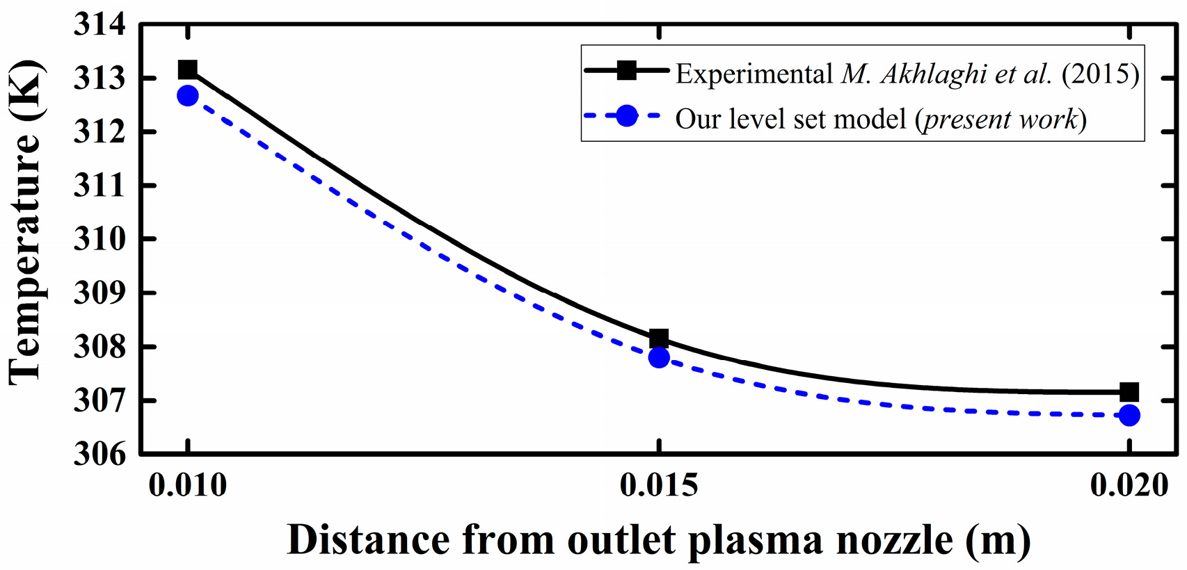
The main aim of the present model was to simulate the mixing phenomena in two-phase fluid systems, which was coupled with the heat transfer module to keep track of temperature dispersion during mixing. In order to exhaustively benchmark the present model, the previous experimental results from Akhlaghi et al. [43] regarding the propagation of plasma plume in ambient air were used, where the measurements were focused on temperature variations versus distance away from the outlet nozzle. Furthermore, experimental data on temperature variations associated with mixing between the discharged plume and the ambient air were needed for the present benchmarking. Therefore, it is remarked that the present experimental benchmarking directly focused on the mixing between the two fluids (in this case plasma plume and air) with subsequent temperature dispersion. In addition, for the sake of benchmarking, a similar experimental setup of Akhlaghi et al. [43] was modeled. The results of this benchmarking are shown in Figure 4.
The results from the present model were in a good agreement with previously obtained experimental data; this proved the capability of the present model to precisely predict the mixing and the subsequent heat distribution during plasma discharge in air. The small deviations between the experimental data and theoretical predictions were likely due to unknown and uncontrollable external factors involved in the experiments.
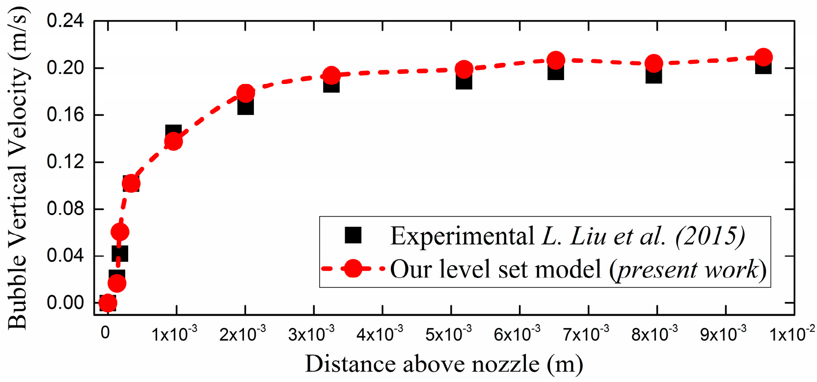
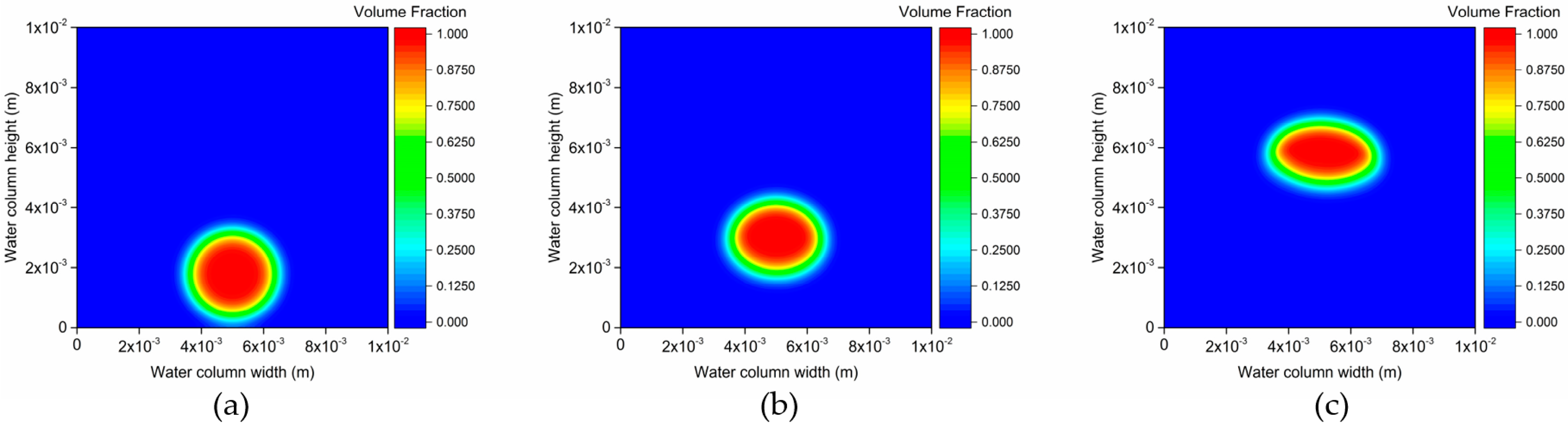
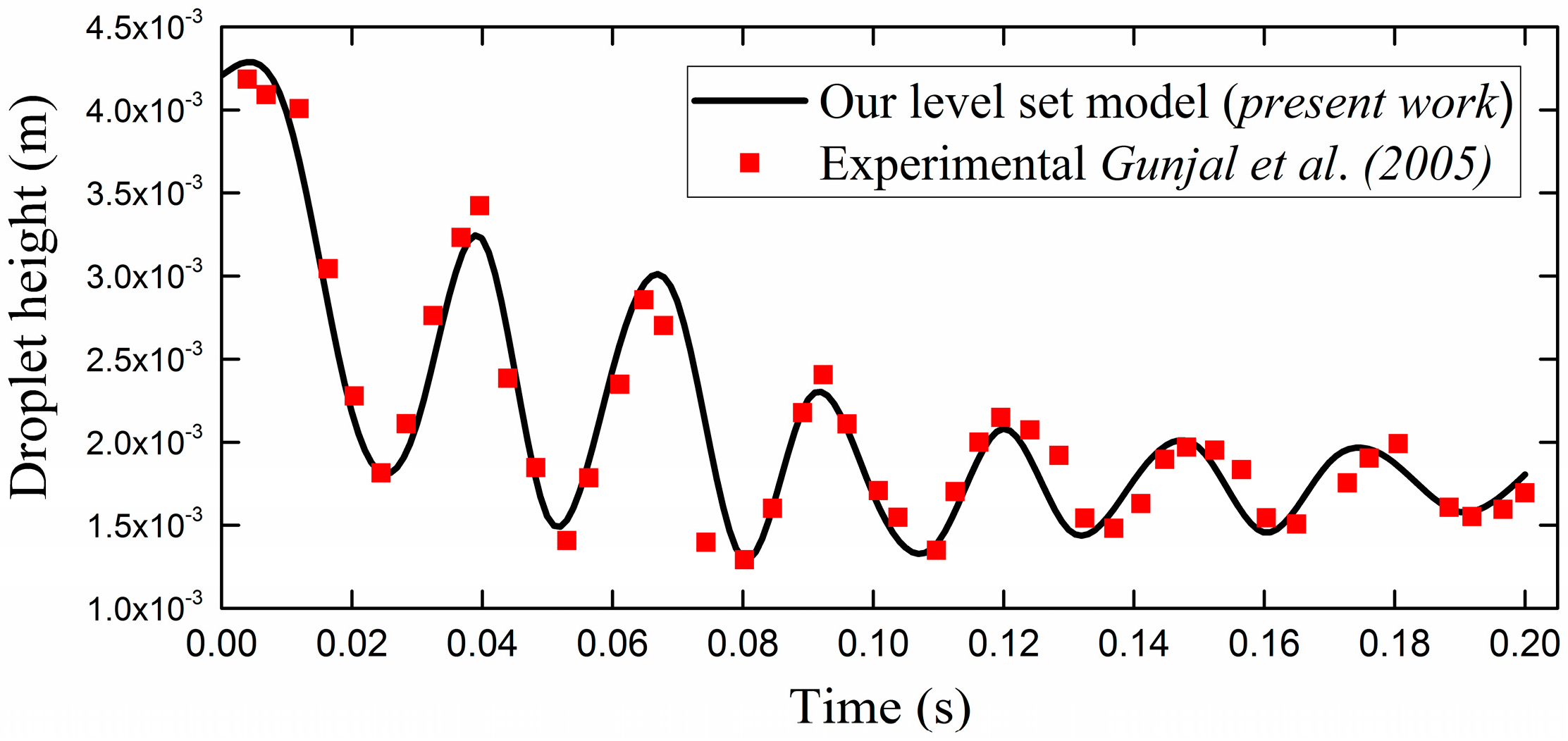
Furthermore, since the present work dealt with mixing of blood (liquid) with helium plasma, the present model was also benchmarked using experimental results with liquid and gas interface, including those for: (1) an air bubble rising in a water column; and (2) a water droplet moving in air and impacting a surface. For (1), the vertical velocities of a 2.77 × 10⁻³ m air bubble at different heights above the bottom nozzle that released the air bubble into the water column were employed [48]. Comparisons between vertical velocities obtained by the experiment and from the present model are shown in Figure 5, which show good agreement. To ensure preservation of the interface between the air bubble and water, the contour plots for the bubble at 0, 0.02 and 0.04 s are shown in Figure 6. The capability of our present model in preserving the interface between the air bubble and water (i.e., the liquid–gas system) was shown. The gradual change in the volume fraction around the air bubble (shown in red) in the water column (shown in blue) demonstrated that the present model could accurately track the degree of mixing between the gas (i.e., air) and the liquid (i.e., water) throughout the simulation. For (2), the variations with time in the height of a 4.2 × 10⁻³-m-diameter water droplet impacting onto a solid surface with a contact angle of 50° [49] were employed. Comparisons between heights obtained by the experiment and from the present model are shown in Figure 7, which show good agreement. The accuracy of the present model in simulating two-phase fluids (i.e., liquid–gas) system was demonstrated by the benchmarking above.
3.2. Computed Results
Due to employment of a finer mesh and a relatively long simulation time of 10.0 s, the present numerical simulation was executed on a computer cluster with Intel® Xeon E5-2670 2.60 GHz using 48 physical cores and hyper-threaded to 96. The computation time to complete the simulations for mixing chambers with and without obstacles was ~2.96 × 10⁴ and ~7.24 × 10³ s, respectively. To make sure that the system had reached the steady-state over the simulation time of 10.0 s, the average velocity in the mixing chamber domain was scored, and the results are shown in Figure 8a,b for chambers with and without obstacles, respectively.
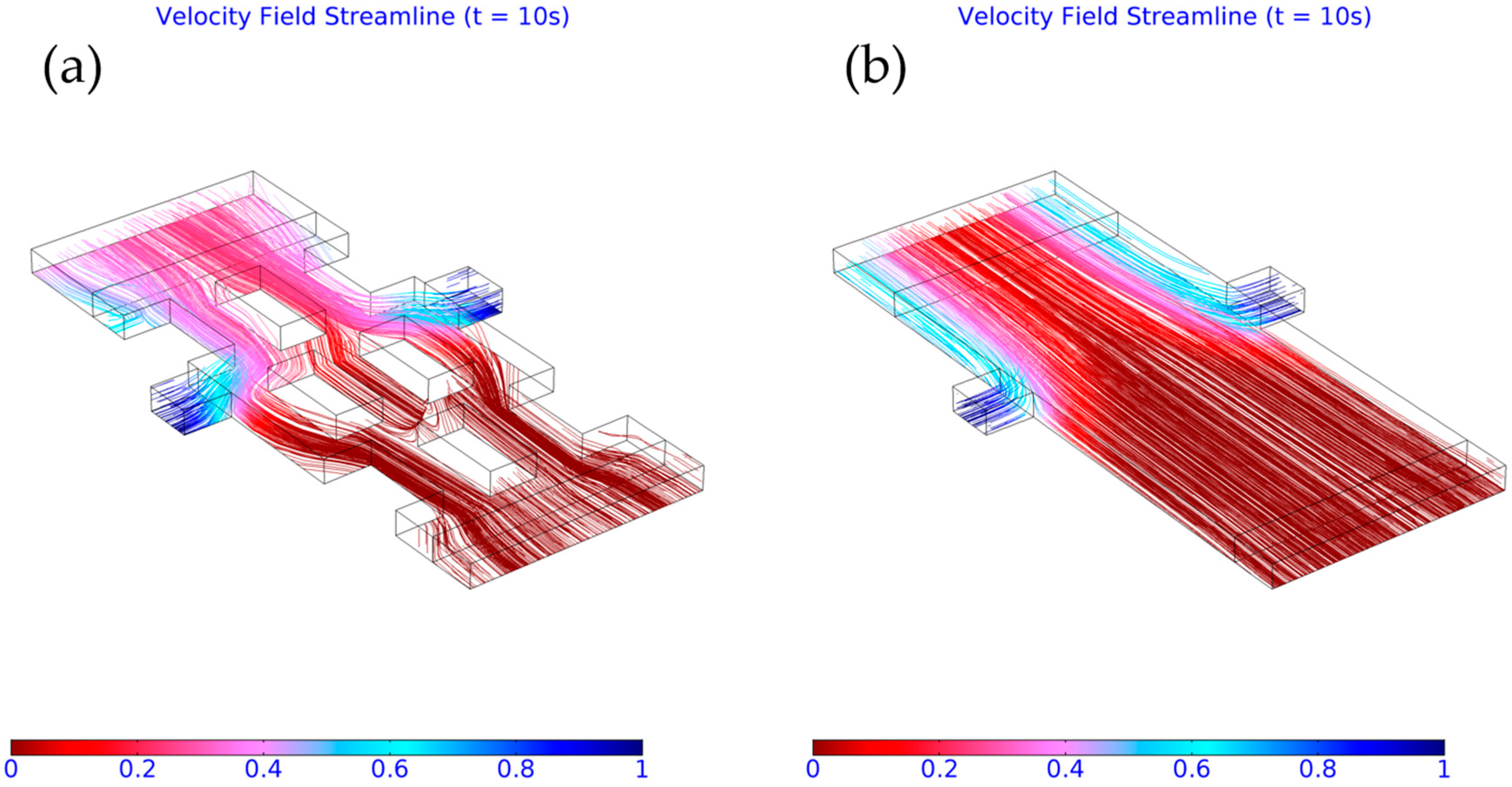
The velocity magnitudes averaged over the mixing chamber domain for the two different conceptual designs of the mixing chamber are shown in Figure 8. The velocities in the mixing chamber domain with obstacles showed fluctuations for t < 2.0 s, mainly due to two reasons: (1) the steady-state was not yet reached for t < 2.0 s; and (2) the presence of obstacles to the flow when chamber was getting filled would significantly affect the flow pattern and the velocity magnitude. In contrast, the velocity variations in the mixing chamber without obstacles were found negligible since a major part of the flow remained undistorted (the center part of the flow that was away from the mixing chamber walls). However, the steady-state for the designs without any obstacles would also be fully achieved at t ~ 2.0 s. After the steady-state was fully achieved, the velocity magnitude in the mixing chamber domain would not fluctuate noticeably. Therefore, the velocity of the flow would remain almost constant while the mixing chamber was in operation (i.e., when the blood and cold plasma were injected from the embedded nozzles). Snapshots for spatial evolution of the velocity over the mixing chamber domains are shown in Figure 9 and Figure 10, for mixing chambers with and without obstacles, respectively.
The spatial evolutions of velocities in the mixing chamber domain are shown in Figure 9 and Figure 10 for mixing chamber with and without obstacles, respectively. For t > 2.0 s, the velocities did not change noticeably. These results together with those shown in Figure 8 supported that steady state was achieved for t > 2.0 s. Moreover, velocities away from the walls were higher than those closer to the no-slip walls due to adhesion between the fluid and solid.
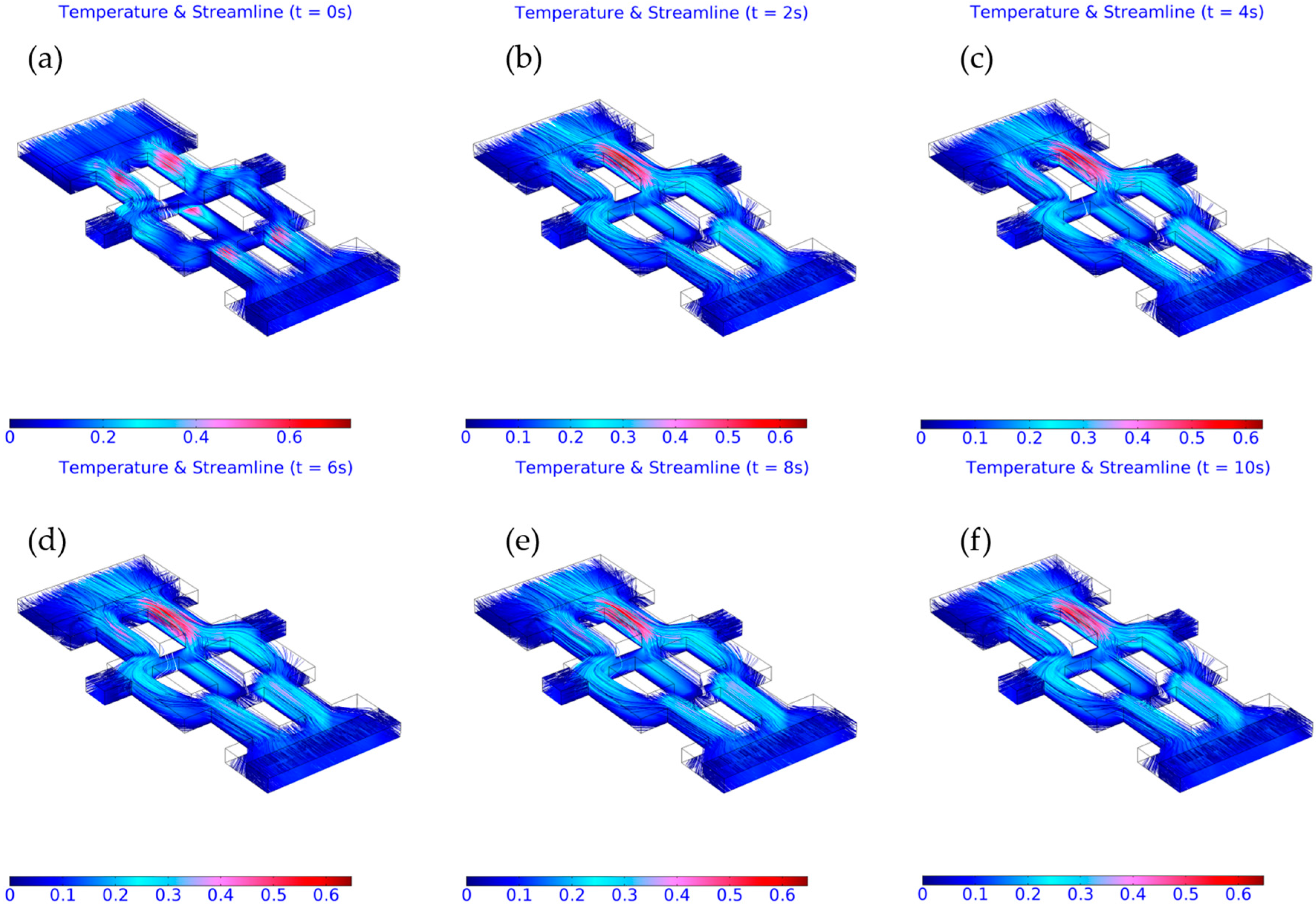
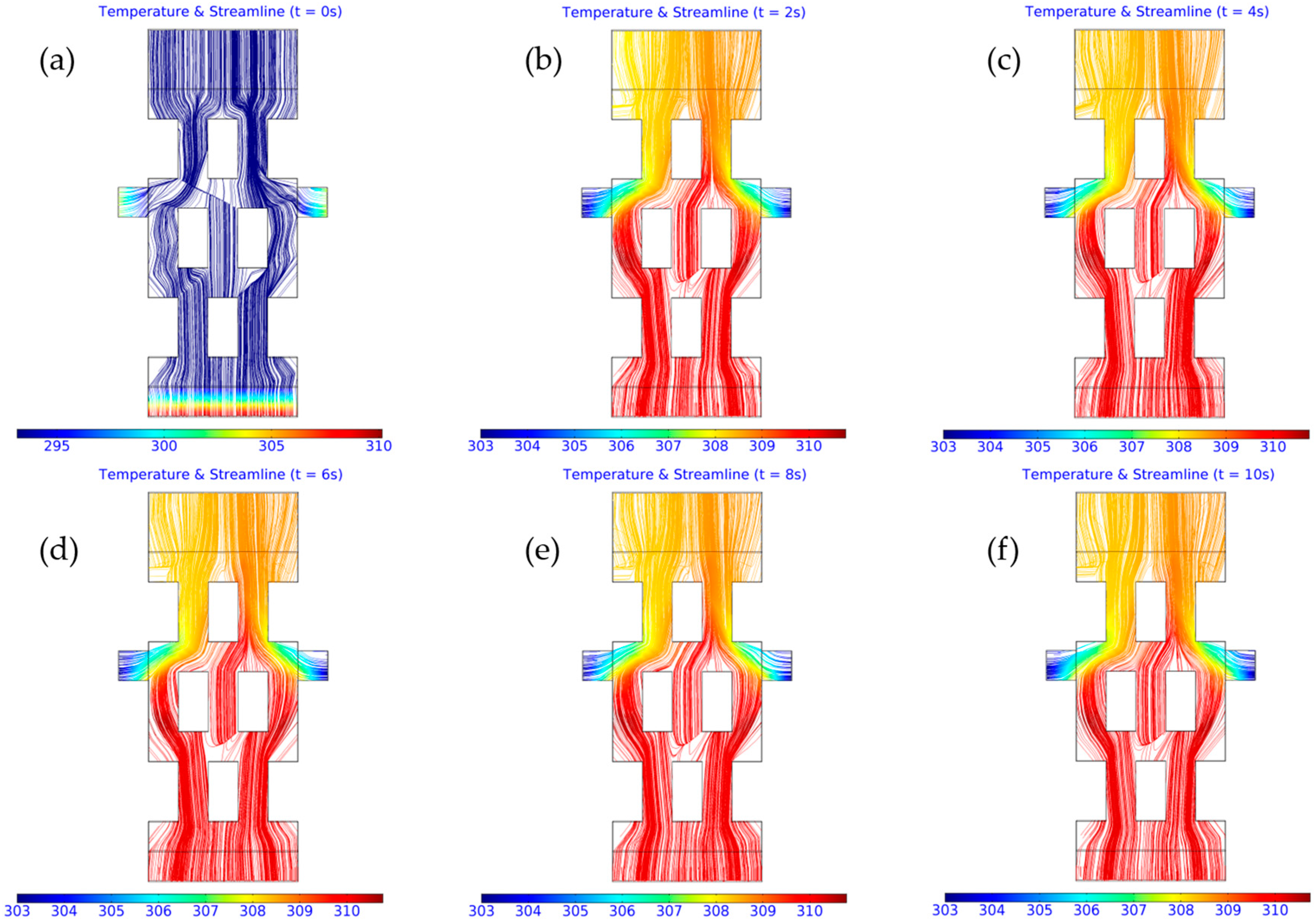
The initial temperature of blood was set to be 310 K [38] and the initial cold plasma temperature was set to be at 303 K [39]. In the FEM technique, an element consisted of a number of nodes, each associated with a shape function (Ni) and a temperature (Ti), so the element temperature would be , where Telement was the temperature in the element, M was the total number of nodes in a specific element, Ni and Ti were the shape function and temperature of the ith node within the element, respectively. The average temperature of the domain was determined through the arithmetic mean of temperatures of elements in the domain. The average temperatures over the outlet nozzle are shown in Figure 11. For t < 2.0 s, the average temperature (i.e., the bulk temperature of the flow) of the mixture in the outlet nozzle domain for the mixing chamber with obstacles was higher than that without obstacles. The increase in the temperature here was explained by the chamber filling and subsequent mixing between the injected blood and plasma. When steady state was achieved after t > ~2.0 s, the average temperature of the mixture in the outlet nozzle domain for both chambers became ~308.55 K. Moreover, the heat transfer between these two different fluids was controlled by the heat flux (q”) and the spatial distribution of temperature, so, as result of the increased contact between blood and plasma in the mixing chamber, the final temperature of the mixture would be regulated based on the initial temperature of both fluids. In addition, it could be concluded that heat transfer could be enhanced by the increased contact as a result of mixing, and at the same time the reaction between the plasma constituents and the blood would be further enhanced. The results of temperature distribution inside the device with the flow streamlines are shown in Figure 12 and Figure 13 for mixing chambers with and without obstacles, respectively. The snapshots were taken from the system every 2.0 s over the total simulation runtime of 10.0 s in which the mixing chamber was fully filled with blood and plasma.
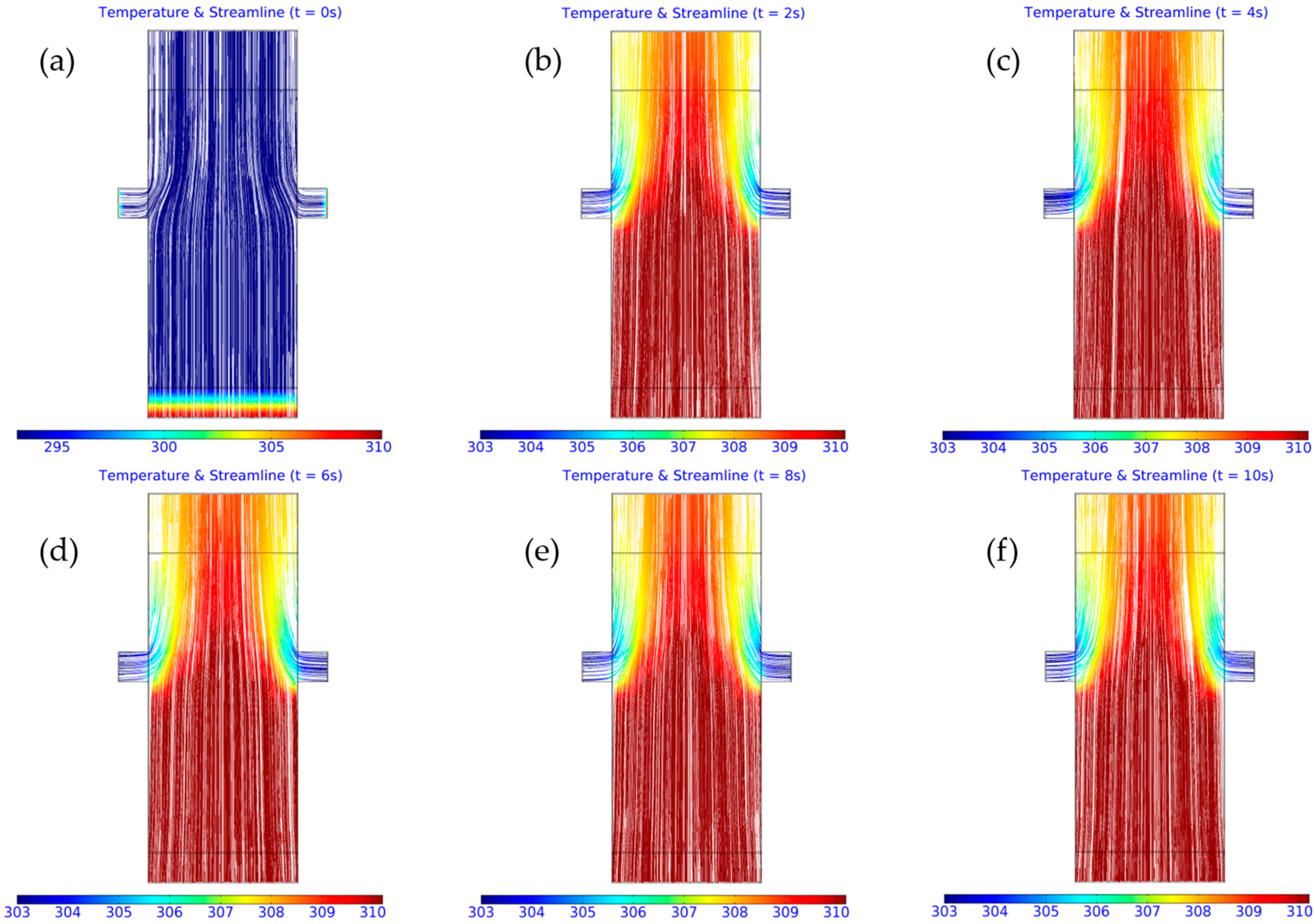
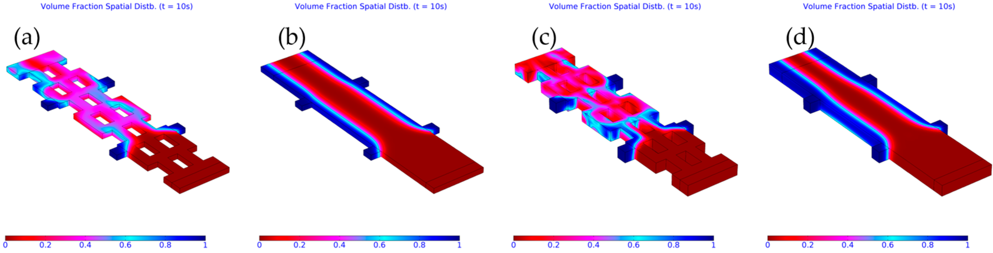
The temperature distributions over the mixing chambers shown in Figure 12 and Figure 13 show the temperature variations between the injected blood and plasma as a result of heat transfer and subsequent mixing. The temperature distributions over the mixing chamber with obstacles were more gradual when compared to those for no obstacles. As shown in Figure 12f, the final mixture temperature at the outlet boundary was ~308 K. The gradual color changes of the flow streamlines characterized the temperature distribution of the mixture of blood and plasma. As observed in Figure 13f, the temperature in the middle part of the outlet nozzle was almost equivalent to the temperature of the injected blood (~310 K). Moreover, the heat distribution tended to be less effective in a mixing chamber without obstacles, as shown in Figure 13f, which did not show gradual changes in the heat color map throughout the device’s domain. In addition, the distribution of blood and plasma volume fractions in both mixing-chamber designs when the chambers are fully filled and when steady-state is reached (i.e., t = 10.0 s) are shown in Figure 14a,b for chambers with and without obstacles, respectively.
The volume fraction near ~0.5 (see color bar in Figure 14) represented a perfect mixing between the two fluids injected into the mixing chamber. Apart from the degree of mixing, special attention would be paid on the spatial distribution of this mixture, which determined the path along which the mixture propagated in a particular mixing-chamber design. As shown by the flow profile Figure 14a, the mixing chamber with obstacles allowed a better mixing and at the same time directed the mixture of blood and plasma into the outlet nozzle. In contrast, the outlet zone in the mixing chamber without obstacles was almost completely filled with blood (see Figure 14b), and the blood at the center of the mixing chamber and the outlet nozzle did not have direct contact with the injected plasma from the side nozzles. In terms of treatment efficiency, it could be expected that the mixing chamber without obstacles would be less effective compared to one with obstacles, since the plasma which was initially present in the system was “pushed out” effectively by the blood without exhaustive mixing due to the higher density and dynamic viscosity of the blood (compared to the injected plasma). The volume fraction at the boundary of the outlet nozzle is quantitatively shown in Figure 15.
The average blood volume fractions scored over the outlet boundary of the nozzle for mixing chambers with and without obstacles are shown in Figure 15. When steady state was achieved after t > ~2.0 s, the results for the two chambers overlapped, which showed that similar amounts of blood exited from the outlets of the chambers. As blood was injected into the chambers, the outlets started to get filled until saturation was reached. The blood volume fraction exiting the outlet boundary was found to be ~0.66 after steady-state was achieved. The spatial distributions of volume fraction in the outlet nozzle for the mixing chambers (at t = 10.0 s) are also shown in Figure 16. Figure 16a shows that the blood and plasma were well-mixed in the presence of obstacles. In contrast, Figure 16b shows that, in the absence of obstacles, mixing was insignificant in the central part of the outlet nozzle, and became more significant towards the side walls of the chamber.
3.3. Importance of Obstacles in Mixing
To the best of our knowledge, there were no reports in the literature on designs on mixing chambers for blood and cold plasma. However, to demonstrate the genericity of the results from using obstacles in mixing chambers and of the corresponding conclusions, three different mixing chamber designs with different dimensions and aspect ratios were analyzed. These chambers had: (a) a long width of 9 × 10⁻² m; (b) small obstacles (1 × 1 × 10−4 m2); and (c) a long length (0.21 m) and two plasma inlets. Schematic diagrams of these chambers are shown in Figure 17a–c. The thicknesses of all chamber designs were set to be either 1 × 10⁻² or 2 × 10⁻² m. As such, each chamber design had four variations with or without obstacles, and with different thicknesses.
Three-dimensional snapshots of mixing chambers with a width of 9 × 10⁻² m having thicknesses of 1 × 10⁻² and 2 × 10⁻² m, with and without obstacles, are shown in Figure 18a–d. Mixing of blood and cold plasma was enhanced by mixing chambers with obstacles when compared to those without obstacles. However, the central part of the mixing chambers was filled with blood not mixed with the injected plasma, which was explained by the insufficient volumetric flow rate of the plasma to achieve adequate mixing. Similarly, three-dimensional snapshots of mixing chambers with small obstacles (1 × 1 × 10−4 m2) having thicknesses of 1 × 10⁻² and 2 × 10⁻² m, with and without obstacles, are shown in Figure 19a–d. Substantial mixing inside the mixing chambers with obstacles was achieved for distances as far as the outlet, which was not affected by an increase in the thickness of the chambers. When no obstacles were present, mixing between blood and plasma was poor and the central part of the mixing chambers was filled with blood not mixed with the injected plasma. Lastly, three-dimensional snapshots of the mixing chambers with a length of 0.21 m and two plasma inlets having thicknesses of 1 × 10⁻² and 2 × 10⁻² m, with and without obstacles, are shown in Figure 20a–d. Similar to previous designs, substantial mixing inside the mixing chambers could only be achieved in the presence of obstacles. According to the above analyses, obstacles within the mixing chambers were generically essential for achieving substantial mixing between the plasma and blood.
4. Conclusions
In the present work, a model based on our previously developed theory [29] was employed to study cold plasma plume mixing with blood with a view to enhance the mixing. The level set method was used to capture the mixing and evolution of blood in cold plasma in two different mixing chamber designs in a three-dimensional coordinate system. Simultaneous determination of temperature distributions in simulated mixing chambers as plasma and blood were injected from the inlet nozzles were enabled by the heat transfer coupling. Enhancement of mixing between blood and plasma in the presence of obstacles to the flow was demonstrated by the present results. The present conceptual designs of mixing chambers would be useful in future development of cold plasma medicine devices for treatment of blood related diseases and at the same time the present model would be an important tool for further investigation of mixing phenomena with subsequent temperature distributions between blood and cold atmospheric pressure plasmas. In addition, the present model could be used to simulate mixing phenomena between the blood and different plasma carrier gases.
Acknowledgments
We acknowledge the support from the Neutron computer cluster from the Department of Physics and Materials Science, City University of Hong Kong, for the computational work involved in this paper. This research was supported by the research grant 7004641 from City University of Hong Kong.
Author Contributions
M.S.B. and K.N.Y. conceived and designed the experiments; M.S.B. and K.N.Y. performed the experiments; M.S.B. and K.N.Y. analyzed the data; M.S.B and K.N.Y. contributed reagents/materials/analysis tools; and M.S.B. and K.N.Y. wrote the paper.
Conflicts of Interest
The authors declare no conflict of interest.
Appendix A
The algorithm of the left-preconditioned GMRES method is described in the following
| Algorithm 1 The left-preconditioned GMRES method |
|
References
- Fridman, G.; Friedman, G.; Gutsol, A.; Shekhter, A.B.; Vasilets, V.N.; Fridman, A. Applied plasma medicine. Plasma Process. Polym. 2008, 5, 503–533. [Google Scholar] [CrossRef]
- Park, G.Y.; Park, S.J.; Choi, M.Y.; Koo, I.G.; Byun, J.H.; Hong, J.W.; Sim, J.Y.; Collins, G.J.; Lee, J.K. Atmospheric-pressure plasma sources for biomedical applications. Plasma Sources Sci. Technol. 2012, 21, 043001. [Google Scholar] [CrossRef]
- Laroussi, M. Low-temperature plasma jet for biomedical applications: A review. IEEE Trans. Plasma Sci. 2015, 43, 703–712. [Google Scholar] [CrossRef]
- Isbary, G.; Morfill, G.; Schmidt, H.U.; Georgi, M.; Ramrath, K.; Heinlin, J.; Karrer, S.; Landthaler, M.; Shimizu, T.; Steffes, B.; et al. A first prospective randomized controlled trial to decrease bacterial load using cold atmospheric argon plasma on chronic wounds in patients. Br. J. Dermatol. 2010, 163, 78–82. [Google Scholar] [CrossRef] [PubMed]
- Arndt, S.; Unger, P.; Wacker, E.; Shimizu, T.; Heinlin, J.; Li, Y.-F.; Thomas, H.M.; Morfill, G.E.; Zimmermann, J.L.; Bosserhoff, A.-K.; et al. Cold atmospheric plasma (CAP) changes gene expression of key molecules of the wound healing machinery and improves wound healing in vitro and in vivo. PLoS ONE 2013, 8, e79325. [Google Scholar] [CrossRef] [PubMed]
- Lee, H.W.; Kim, G.J.; Kim, J.M.; Park, J.K.; Lee, J.K.; Kim, G.C. Tooth bleaching with nonthermal atmospheric pressure plasma. J. Endod. 2009, 35, 587–591. [Google Scholar] [CrossRef] [PubMed]
- Cheng, X.; Murphy, W.; Recek, N.; Yan, D.; Cvelbar, U.; Vesel, A.; Mozetič, M.; Canady, J.; Keidar, M.; Sherman, J.H. Synergistic effect of gold nanoparticles and cold plasma on glioblastoma cancer therapy. J. Phys. D Appl. Phys. 2014, 47, 335402. [Google Scholar] [CrossRef]
- Cheng, X.; Sherman, J.; Murphy, W.; Ratovitski, E.; Canady, J.; Keidar, M. The Effect of Tuning Cold Plasma Composition on Glioblastoma Cell Viability. PLoS ONE 2014, 9, e98652. [Google Scholar] [CrossRef] [PubMed]
- Yan, D.; Talbot, A.; Nourmohammadi, N.; Cheng, X.; Canady, J.; Sherman, J.; Keidar, M. Principles of using cold atmospheric plasma stimulated media for cancer treatment. Sci. Rep. 2015, 5, 18339. [Google Scholar] [CrossRef] [PubMed]
- Rupf, S.; Lehmann, A.; Hannig, M.; Schäfer, B.; Schubert, A.; Feldmann, U.; Schindler, A. Killing of adherent oral microbes by a non-thermal atmospheric plasma jet. J. Med. Microbiol. 2010, 59, 206–212. [Google Scholar] [CrossRef] [PubMed]
- Noriega, E.; Shama, G.; Laca, A.; Díaz, M.; Kong, M.G. Cold atmospheric gas plasma disinfection of chicken meat and chicken skin contaminated with Listeria innocua. Food Microbiol. 2011, 28, 1293–1300. [Google Scholar] [CrossRef] [PubMed]
- Nishime, T.M.; Borges, A.C.; Koga-Ito, C.Y.; Machida, M.; Hein, L.R.; Kostov, K.G. Non-thermal atmospheric pressure plasma jet applied to inactivation of different microorganisms. Surf. Coat. Technol. 2017, 312, 19–24. [Google Scholar] [CrossRef]
- Ermolaeva, S.A.; Petrov, O.F.; Naroditsky, B.S.; Fortov, V.E.; Morfill, G.E.; Gintsburg, A.L. Cold Plasma Therapy. Ref. Modul. Biomed. Sci. Compr. Biomed. Phys. 2014, 10, 343–367. [Google Scholar]
- Preedy, E.C.; Brousseau, E.; Evans, S.L.; Perni, S.; Prokopovich, P. Adhesive forces and surface properties of cold gas plasma treated UHMWPE. Coll. Surf. A Physicochem. Eng. Asp. 2014, 460, 83–89. [Google Scholar] [CrossRef] [PubMed]
- Perni, S.; Kong, M.G.; Prokopovich, P. Cold atmospheric pressure gas plasma enhances the wear performance of ultra-high molecular weight polyethylene. Acta Biomater. 2012, 8, 1357–1365. [Google Scholar] [CrossRef] [PubMed]
- Raiser, J.; Zenker, M. Argon plasma coagulation for open surgical and endoscopic applications: State of the art. J. Phys. D Appl. Phys. 2006, 39, 3520–3523. [Google Scholar] [CrossRef]
- Fridman, G.; Peddinghaus, M.; Balasubramanian, M.; Ayan, H.; Fridman, A.; Gutsol, A.; Brooks, A. Blood coagulation and living tissue sterilization by floating-electrode dielectric barrier discharge in air. Plasma Chem. Plasma Process. 2006, 26, 425–442. [Google Scholar] [CrossRef]
- Dobrynin, D.; Fridman, G.; Friedman, G.; Fridman, A. Physical and biological mechanisms of direct plasma interaction with living tissue. New J. Phys. 2009, 11, 115020. [Google Scholar] [CrossRef]
- Morfill, G.E.; Kong, M.G.; Zimmermann, J.L. Focus on plasma medicine. New J. Phys. 2009, 11, 115011. [Google Scholar] [CrossRef]
- Bekeschus, S.; Masur, K.; Kolata, J.; Wende, K.; Schmidt, A.; Bundscherer, L.; Barton, A.; Kramer, A.; Bröker, B.; Weltmann, K.D. Human mononuclear cell survival and proliferation is modulated by cold atmospheric plasma jet. Plasma Process. Polym. 2013, 10706–10713. [Google Scholar] [CrossRef]
- Hung, Y.W.; Lee, L.T.; Peng, Y.C.; Chang, C.T.; Wong, Y.K.; Tung, K.C. Effect of a nonthermal-atmospheric pressure plasma jet on wound healing: An animal study. J. China Med. Assoc. 2016, 79, 320–328. [Google Scholar] [CrossRef] [PubMed]
- Barekzi, N.; Laroussi, M. Dose-dependent killing of leukemia cells by low-temperature plasma. J. Phys. D Appl. Phys. 2012, 45, 422002. [Google Scholar] [CrossRef]
- Kalghatgi, S.U.; Fridman, G.; Cooper, M.; Nagaraj, G.; Peddinghaus, M.; Balasubramanian, M.; Vasilets, V.N.; Gutsol, A.F.; Fridman, A.; Friedman, G. Mechanism of blood coagulation by nonthermal atmospheric pressure dielectric barrier discharge plasma. IEEE Trans. Plasma Sci. 2007, 35, 1559–1566. [Google Scholar] [CrossRef]
- Chen, Z.; Cheng, X.; Lin, L.; Keidar, M. Cold atmospheric plasma discharged in water and its potential use in cancer therapy. J. Phys. D Appl. Phys. 2017, 50, 015208. [Google Scholar] [CrossRef]
- Shimizu, T.; Steffes, B.; Pompl, R.; Jamitzky, F.; Bunk, W.; Ramrath, K.; Georgi, M.; Stolz, W.; Schmidt, H-.U.; Urayama, T.; et al. Characterization of microwave plasma torch for decontamination. Plasma Process. Polym. 2008, 5, 577–582. [Google Scholar] [CrossRef]
- Khan, F.U.; Rehman, N.U.; Naseer, S.; Naz, M.Y.; Khattak, N.A.; Zakaullah, M. Effect of excitation and vibrational temperature on the dissociation of nitrogen molecules in Ar-N2 mixture RF discharge. Spectrosc. Lett. 2011, 44, 194–202. [Google Scholar] [CrossRef]
- Laroussi, M.; Lu, X. Room-temperature atmospheric pressure plasma plume for biomedical applications. Appl. Phys. Lett. 2005, 87, 113902. [Google Scholar] [CrossRef]
- Shahmohammadi Beni, M.; Yu, K.N. Safeguarding against inactivation temperatures during plasma treatment of skin: Multiphysics model and phase field method. Math. Comput. Appl. 2017, 22, 24. [Google Scholar] [CrossRef]
- Shahmohammadi Beni, M.; Yu, K.N. Computational fluid dynamics analysis of cold plasma carrier gas injected into a fluid using level set method. Biointerphases 2015, 10, 041003. [Google Scholar] [CrossRef] [PubMed]
- Schröder, M.; Ochoa, A.; Breitkopf, C. Numerical simulation of an atmospheric pressure RF-driven plasma needle and heat transfer to adjacent human skin using COMSOL. Biointerphases 2015, 10, 029508. [Google Scholar] [CrossRef] [PubMed]
- Sakiyama, Y.; Graves, D.B. Finite element analysis of an atmospheric pressure RF-excited plasma needle. J. Phys. D Appl. Phys. 2006, 39, 3451–3456. [Google Scholar] [CrossRef]
- Sakiyama, Y.; Graves, D.B. Corona-glow transition in the atmospheric pressure RF-excited plasma needle. J. Phys. D Appl. Phys. 2006, 39, 3644–3652. [Google Scholar] [CrossRef]
- Olsson, E.; Kreiss, G. A conservative level set method for two phase flow. J. Comput. Phys. 2005, 210, 225–246. [Google Scholar] [CrossRef]
- Olsson, E.; Kreiss, G.; Zahedi, S. A conservative level set method for two phase flow II. J. Comput. Phys. 2007, 225, 785–807. [Google Scholar] [CrossRef]
- Sussman, M.; Fatemi, E.; Smereka, P.; Osher, S. An improved level set method for incompressible two-phase flows. Comput. Fluids 1998, 27, 663–680. [Google Scholar] [CrossRef]
- Zahedi, S.; Gustavsson, K.; Kreiss, G. A conservative level set method for contact line dynamics. J. Comput. Phys. 2009, 228, 6361–6375. [Google Scholar] [CrossRef]
- Morris, P.D.; Narracott, A.; von Tengg-Kobligk, H.; Soto, D.A.; Hsiao, S.; Lungu, A.; Evans, P.; Bressloff, N.W.; Lawford, P.V.; Hose, D.R.; et al. Computational fluid dynamics modelling in cardiovascular medicine. Heart 2016, 102, 18–28. [Google Scholar] [CrossRef] [PubMed]
- González-Alonso, J.; Calbet, J.A.; Boushel, R.; Helge, J.W.; Søndergaard, H.; Munch-Andersen, T.; Hall, G.; Mortensen, S.P.; Secher, N.H. Blood temperature and perfusion to exercising and non-exercising human limbs. Exp. Physiol. 2015, 100, 1118–1131. [Google Scholar] [CrossRef] [PubMed]
- Shashurin, A.; Keidar, M.; Bronnikov, S.; Jurjus, R.A.; Stepp, M.A. Living tissue under treatment of cold plasma atmospheric jet. Appl. Phys. Lett. 2008, 93, 181501. [Google Scholar] [CrossRef]
- Saad, Y.; Schultz, M.H. GMRES: A generalized minimal residual algorithm for solving nonsymmetric linear systems. SIAM J. Sci. Stat. Comput. 1986, 7, 856–869. [Google Scholar] [CrossRef]
- MPICH Package. Available online: http://www.mpich.org (accessed on 22 February 2017).
- Davies, B.; Morris, T. Physiological parameters in laboratory animals and humans. Pharm. Res. 1993, 10, 1093–1095. [Google Scholar] [CrossRef] [PubMed]
- Akhlaghi, M.; Rajayi, H.; Shahriar Mashayekh, A.; Khani, M.; Mohammad Hassan, Z.; Shokri, B. On the design and characterization of a new cold atmospheric pressure plasma jet and its applications on cancer cells treatment. Biointerphases 2015, 10, 029510. [Google Scholar] [CrossRef] [PubMed]
- Hinghofer-Szalkay, H.; Greenleaf, J.E. Continuous monitoring of blood volume changes in humans. J. Appl. Physiol. 1987, 63, 1003–1007. [Google Scholar] [PubMed]
- Johnson, J.M.; Brengelmann, G.L.; Hales, J.R.; Vanhoutte, P.M.; Wenger, C.B. Regulation of the cutaneous circulation. Fed. Proc. 1986, 45, 2841–2850. [Google Scholar] [PubMed]
- Kalozoumis, P.G.; Kalfas, A.I.; Giannoukas, A.D. The role of geometry of the human carotid bifurcation in the formation and development of atherosclerotic plaque. In Proceedings of the XII Mediterranean Conference on Medical and Biological Engineering and Computing, Chalkidiki, Greece, 27–30 May 2010; Volume 29, pp. 284–287. [Google Scholar]
- V 20 Committee. Standard for Verification and Validation in Computational Fluid Dynamics and Heat Transfer; American Society of Mechanical Engineers: New York, NY, USA, 2009. [Google Scholar]
- Liu, L.; Yan, H.; Zhao, G. Experimental studies on the shape and motion of air bubbles in viscous liquids. Exp. Therm. Fluid Sci. 2015, 62, 109–121. [Google Scholar] [CrossRef]
- Gunjal, P.R.; Ranade, V.V.; Chaudhari, R.V. Dynamics of drop impact on solid surface: Experiments and VOF simulations. AlChE J. 2005, 51, 59–78. [Google Scholar] [CrossRef]
Figure 1.
Mixing chambers (a) with and (b) without obstacles, with inlets and outlets shown.
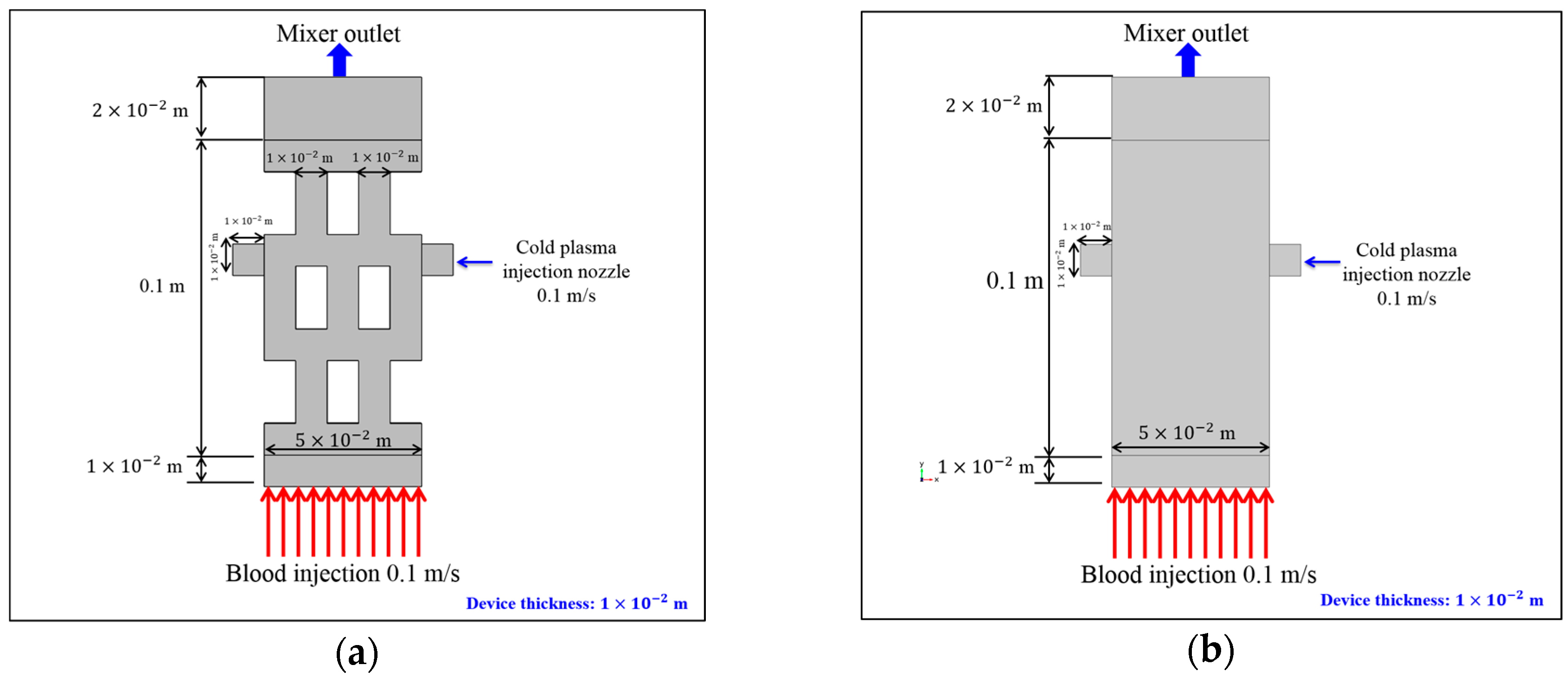
Figure 2.
Seamless mesh employed for two mixing chambers with different configurations.
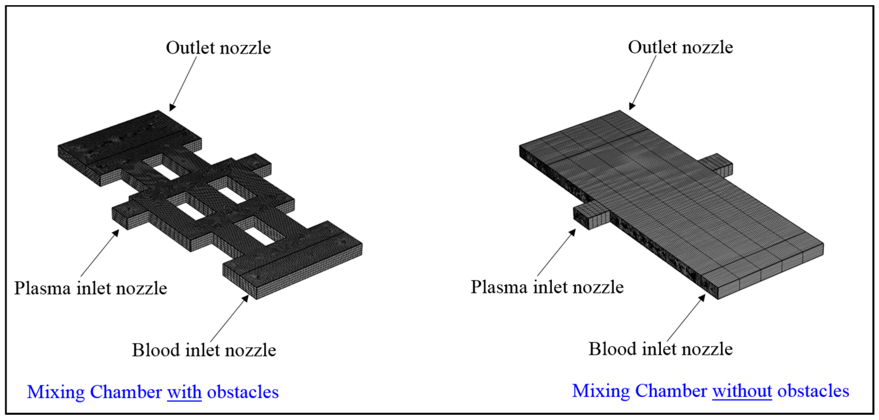
Figure 3.
Grid sensitivity analysis (GSA) for: (a) blood volume fraction exiting the outlet boundary of the mixing chamber; and (b) temperature of the outlet nozzle for chosen average grid sizes of 2 × 10⁻⁴, 1 × 10⁻⁴ and 3 × 10⁻⁵ m.
Figure 3.
Grid sensitivity analysis (GSA) for: (a) blood volume fraction exiting the outlet boundary of the mixing chamber; and (b) temperature of the outlet nozzle for chosen average grid sizes of 2 × 10⁻⁴, 1 × 10⁻⁴ and 3 × 10⁻⁵ m.
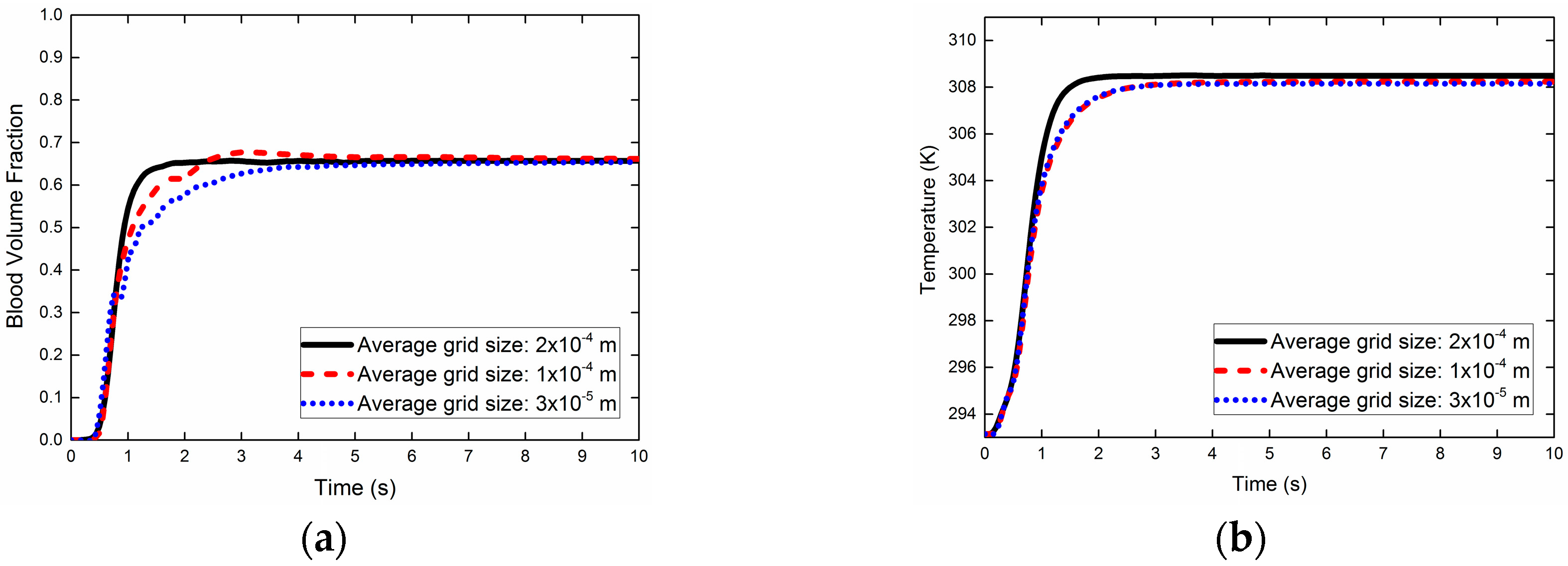
Figure 4.
Comparison between temperatures at different distances from the outlet for 6 kV operating voltage obtained experimentally by Akhlaghi et al. [43] and from theoretical predictions.
Figure 4.
Comparison between temperatures at different distances from the outlet for 6 kV operating voltage obtained experimentally by Akhlaghi et al. [43] and from theoretical predictions.

Figure 5.
Comparisons between vertical velocities of a 2.77 × 10⁻³ m air bubble at different heights above the bottom nozzle that released the air bubble into the water column obtained experimentally [48] (squares) and from the present model (circles).
Figure 5.
Comparisons between vertical velocities of a 2.77 × 10⁻³ m air bubble at different heights above the bottom nozzle that released the air bubble into the water column obtained experimentally [48] (squares) and from the present model (circles).

Figure 6.
Contour plots of the 2.77 × 10⁻³ m air bubble rising through the water column at: (a) 0; (b) 0.02; and (c) 0.04 s. Blue color represents water and red color represents the air bubble.
Figure 6.
Contour plots of the 2.77 × 10⁻³ m air bubble rising through the water column at: (a) 0; (b) 0.02; and (c) 0.04 s. Blue color represents water and red color represents the air bubble.

Figure 7.
Comparisons between the heights of a 4.2 × 10⁻³-m-diameter water droplet impacting onto a solid surface with a contact angle of 50° [49] (squares) and from the present model (curve).
Figure 7.
Comparisons between the heights of a 4.2 × 10⁻³-m-diameter water droplet impacting onto a solid surface with a contact angle of 50° [49] (squares) and from the present model (curve).

Figure 8.
Average velocity magnitude of the mixture of fluids over the mixing chamber domain with and without obstacles (Note: the mixing chamber domain is marked in blue).
Figure 8.
Average velocity magnitude of the mixture of fluids over the mixing chamber domain with and without obstacles (Note: the mixing chamber domain is marked in blue).
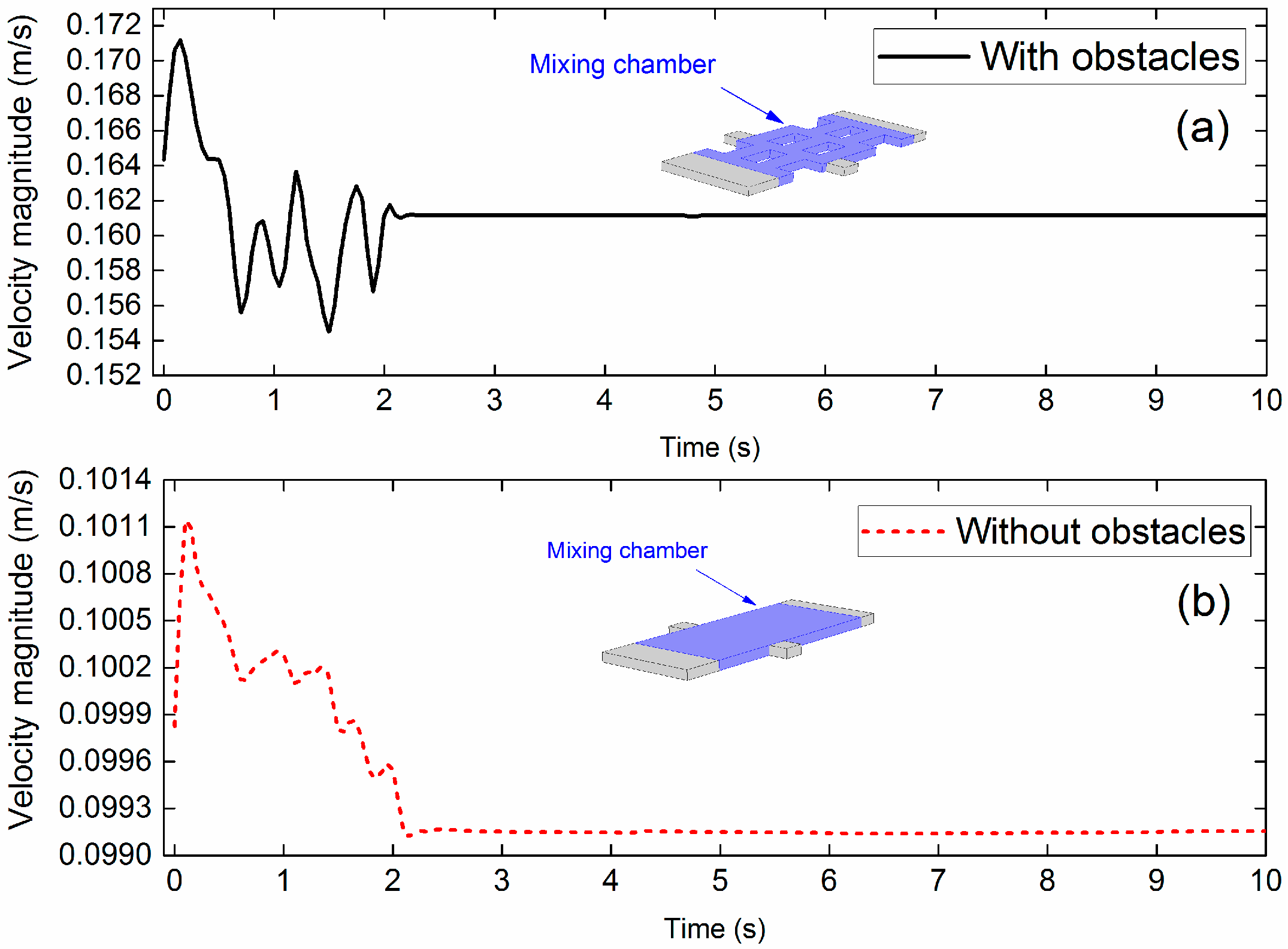
Figure 9.
Distribution of velocity streamlines over the mixing chamber with obstacles at: (a) 0 s; (b) 2 s; (c) 4 s; (d) 6 s; (e) 8 s; and (f) 10 s. Different velocities are represented by different colors as shown in the color bar (in m s−1).
Figure 9.
Distribution of velocity streamlines over the mixing chamber with obstacles at: (a) 0 s; (b) 2 s; (c) 4 s; (d) 6 s; (e) 8 s; and (f) 10 s. Different velocities are represented by different colors as shown in the color bar (in m s−1).

Figure 10.
Distribution of velocity streamlines over the mixing chamber without obstacles at: (a) 0 s; (b) 2 s; (c) 4 s; (d) 6 s; (e) 8 s; and (f) 10 s. Different velocities are represented by different colors as shown in the color bar (in m s−1).
Figure 10.
Distribution of velocity streamlines over the mixing chamber without obstacles at: (a) 0 s; (b) 2 s; (c) 4 s; (d) 6 s; (e) 8 s; and (f) 10 s. Different velocities are represented by different colors as shown in the color bar (in m s−1).
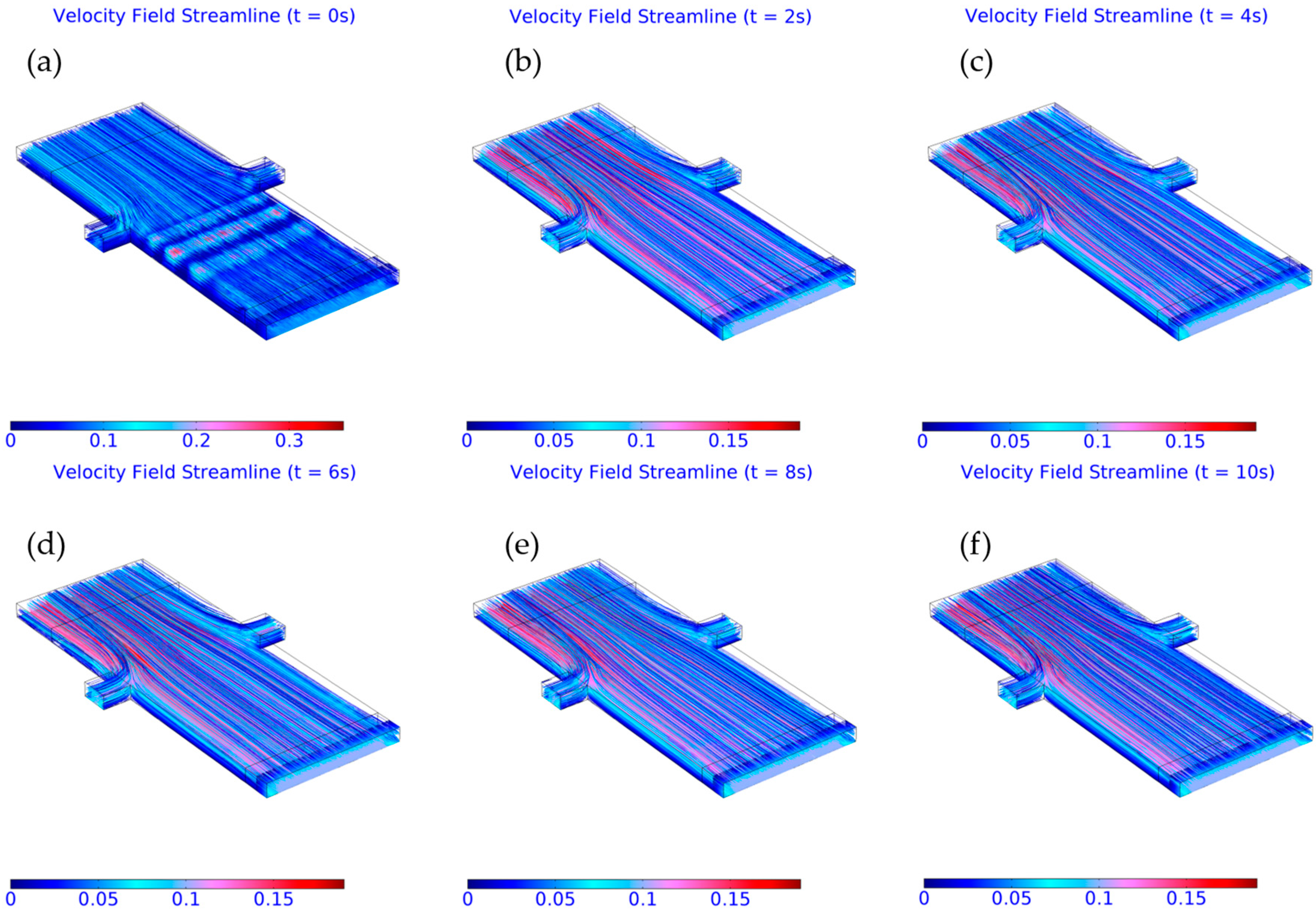
Figure 11.
Average temperature of mixture over outlet nozzle domain (shown in blue) for mixing chambers with and without obstacles (Note: outlet nozzle domain is marked in blue).
Figure 11.
Average temperature of mixture over outlet nozzle domain (shown in blue) for mixing chambers with and without obstacles (Note: outlet nozzle domain is marked in blue).
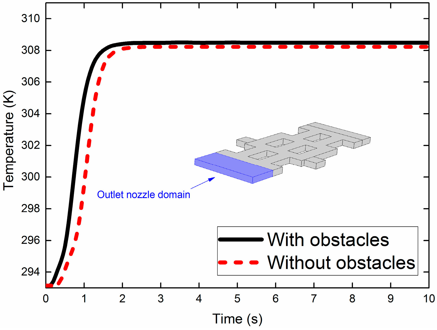
Figure 12.
Distribution of flow streamlines and temperature over the mixing chamber with obstacles at: (a) 0 s; (b) 2 s; (c) 4 s; (d) 6 s; (e) 8 s; and (f) 10 s. Different temperatures are represented by different colors as shown in the color bar (in K).
Figure 12.
Distribution of flow streamlines and temperature over the mixing chamber with obstacles at: (a) 0 s; (b) 2 s; (c) 4 s; (d) 6 s; (e) 8 s; and (f) 10 s. Different temperatures are represented by different colors as shown in the color bar (in K).

Figure 13.
Distribution of flow streamlines and temperature over the mixing chamber without obstacles at: (a) 0 s; (b) 2 s; (c) 4 s; (d) 6 s; (e) 8 s; and (f) 10 s. Different temperatures are represented by different colors as shown in the color bar (in K).
Figure 13.
Distribution of flow streamlines and temperature over the mixing chamber without obstacles at: (a) 0 s; (b) 2 s; (c) 4 s; (d) 6 s; (e) 8 s; and (f) 10 s. Different temperatures are represented by different colors as shown in the color bar (in K).

Figure 14.
Distributions of mixture volume fractions (between 0 and 1) in mixing chambers: (a) with obstacles; and (b) without obstacles. The colors represent the volume fractions of the mixture; red corresponds to the blood (volume fraction = 0) and blue corresponds the plasma (volume fraction = 1).

Figure 15.
Average blood volume fractions scored over the outlet boundary of the nozzle (shown in blue) for mixing chambers with and without obstacles.
Figure 15.
Average blood volume fractions scored over the outlet boundary of the nozzle (shown in blue) for mixing chambers with and without obstacles.
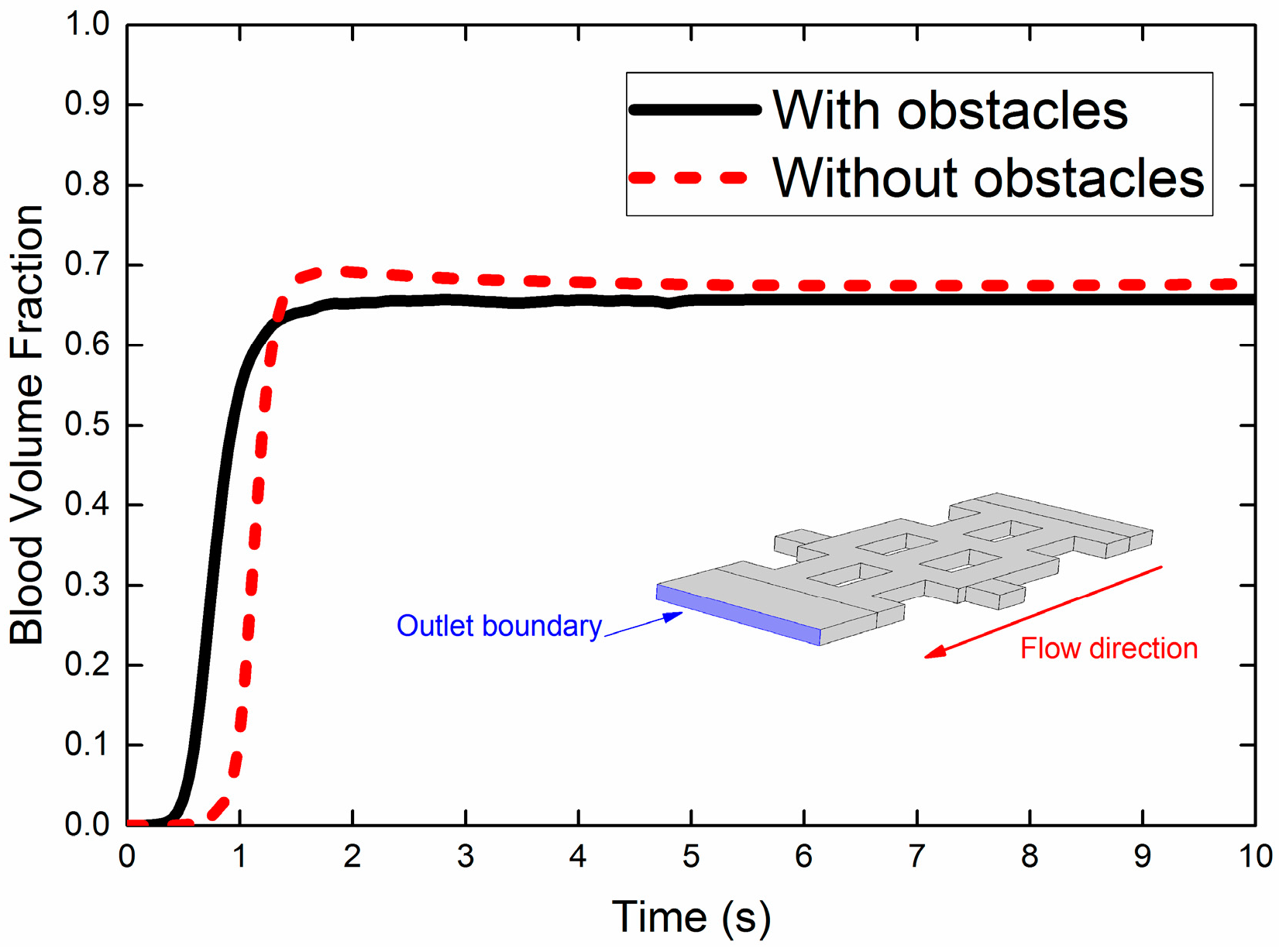
Figure 16.
Spatial distributions of volume fraction in the outlet nozzle for mixing chamber: (a) with obstacles; and (b) without obstacles at 10.0 s. Blue color (i.e., volume fraction = 0) represents blood while red color (i.e., volume fraction = 1) represents plasma.
Figure 16.
Spatial distributions of volume fraction in the outlet nozzle for mixing chamber: (a) with obstacles; and (b) without obstacles at 10.0 s. Blue color (i.e., volume fraction = 0) represents blood while red color (i.e., volume fraction = 1) represents plasma.
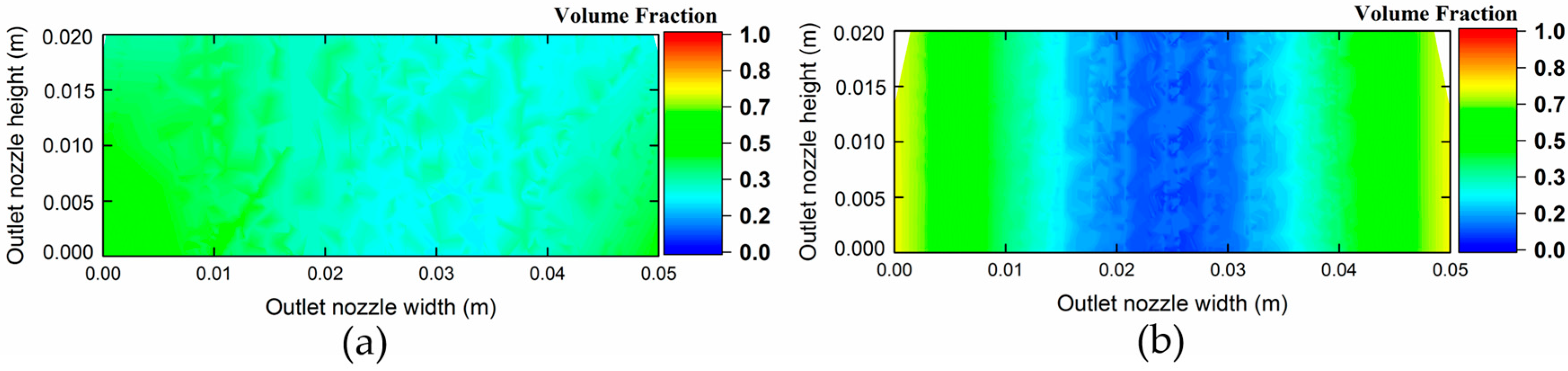
Figure 17.
Schematic diagrams of mixing chambers with: (a) a long width of 9 × 10⁻² m; (b) smaller obstacles (1 × 1 × 10−4 m2); and (c) a long length (0.21 m) and two plasma inlets.
Figure 17.
Schematic diagrams of mixing chambers with: (a) a long width of 9 × 10⁻² m; (b) smaller obstacles (1 × 1 × 10−4 m2); and (c) a long length (0.21 m) and two plasma inlets.
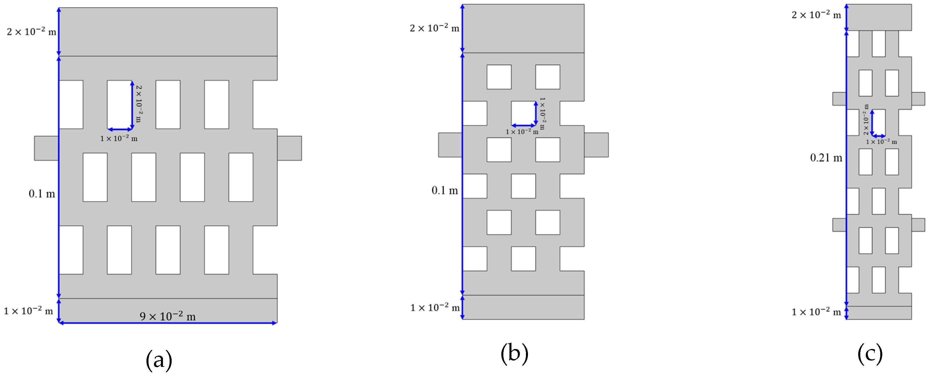
Figure 18.
Three-dimensional snapshots of mixing chambers with a width of 9 × 10⁻² m having a thickness of 1 × 10⁻² m: (a) with obstacles; and (b) without obstacles; and having a thickness of 2 × 10⁻² m: (c) with obstacles; and (d) without obstacles.
Figure 18.
Three-dimensional snapshots of mixing chambers with a width of 9 × 10⁻² m having a thickness of 1 × 10⁻² m: (a) with obstacles; and (b) without obstacles; and having a thickness of 2 × 10⁻² m: (c) with obstacles; and (d) without obstacles.
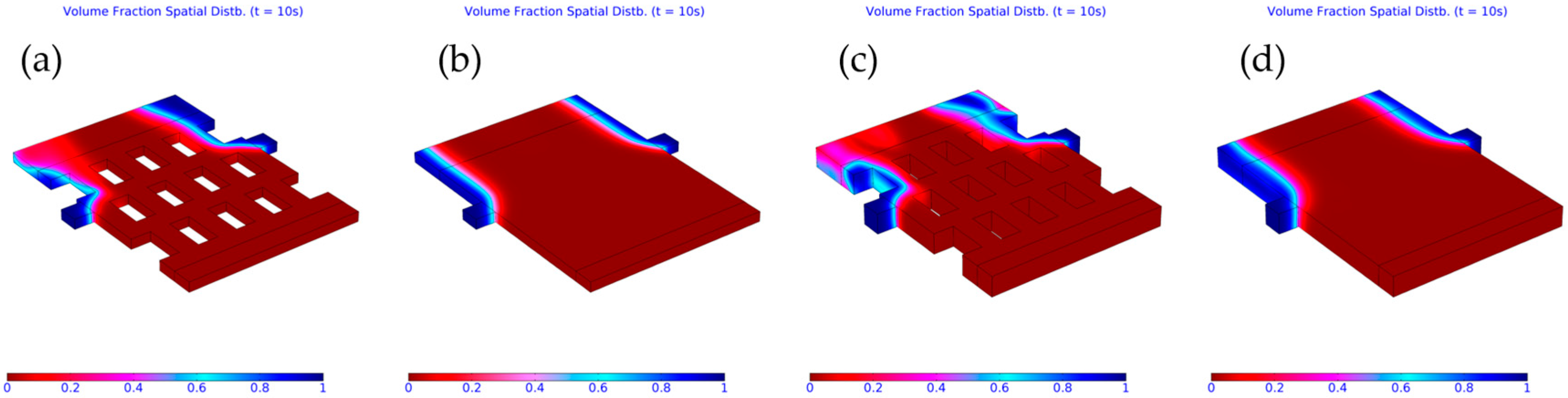
Figure 19.
Three-dimensional snapshots of mixing chambers with small obstacles (1 × 1 × 10−4 m2) having a thickness of 1 × 10⁻² m: (a) with obstacles; and (b) without obstacles; and having a thickness of 2 × 10⁻² m: (c) with obstacles; and (d) without obstacles.
Figure 19.
Three-dimensional snapshots of mixing chambers with small obstacles (1 × 1 × 10−4 m2) having a thickness of 1 × 10⁻² m: (a) with obstacles; and (b) without obstacles; and having a thickness of 2 × 10⁻² m: (c) with obstacles; and (d) without obstacles.
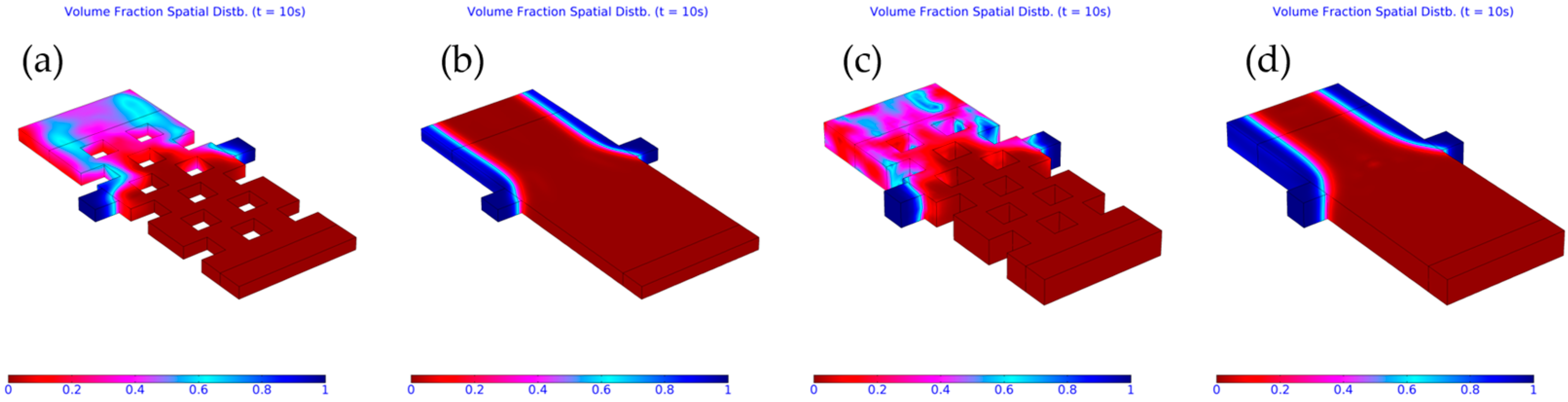
Figure 20.
Three-dimensional snapshots of mixing chambers with a length of 0.21 m and two plasma inlets having a thickness of 1 × 10⁻² m: (a) with obstacles; and (b) without obstacles; and having a thickness of 2 × 10⁻² m: (c) with obstacles; and (d) without obstacles.
Figure 20.
Three-dimensional snapshots of mixing chambers with a length of 0.21 m and two plasma inlets having a thickness of 1 × 10⁻² m: (a) with obstacles; and (b) without obstacles; and having a thickness of 2 × 10⁻² m: (c) with obstacles; and (d) without obstacles.


© 2017 by the authors. Licensee MDPI, Basel, Switzerland. This article is an open access article distributed under the terms and conditions of the Creative Commons Attribution (CC BY) license (http://creativecommons.org/licenses/by/4.0/).
Share and Cite
MDPI and ACS Style
Shahmohammadi Beni, M.; Yu, K.N. Computational Fluid Dynamics Analysis of Cold Plasma Plume Mixing with Blood Using Level Set Method Coupled with Heat Transfer. Appl. Sci. 2017, 7, 578. https://doi.org/10.3390/app7060578
AMA Style
Shahmohammadi Beni M, Yu KN. Computational Fluid Dynamics Analysis of Cold Plasma Plume Mixing with Blood Using Level Set Method Coupled with Heat Transfer. Applied Sciences. 2017; 7(6):578. https://doi.org/10.3390/app7060578
Chicago/Turabian StyleShahmohammadi Beni, Mehrdad, and Kwan Ngok Yu. 2017. "Computational Fluid Dynamics Analysis of Cold Plasma Plume Mixing with Blood Using Level Set Method Coupled with Heat Transfer" Applied Sciences 7, no. 6: 578. https://doi.org/10.3390/app7060578
Note that from the first issue of 2016, this journal uses article numbers instead of page numbers. See further details here.