
Composite Kernel Method for PolSAR Image Classification Based on Polarimetric-Spatial Information


1
Center for Information Geoscience, University of Electronic Science and Technology of China, Chengdu 611731, China
2
Huiding Technology Co. Ltd., Chengdu 611731, China
*
Author to whom correspondence should be addressed.
Appl. Sci. 2017, 7(6), 612; https://doi.org/10.3390/app7060612
Submission received: 14 April 2017
/
Revised: 31 May 2017
/
Accepted: 9 June 2017
/
Published: 13 June 2017
(This article belongs to the Special Issue Polarimetric SAR Techniques and Applications)
Abstract
:The composite kernel feature fusion proposed in this paper attempts to solve the problem of classifying polarimetric synthetic aperture radar (PolSAR) images. Here, PolSAR images take into account both polarimetric and spatial information. Various polarimetric signatures are collected to form the polarimetric feature space, and the morphological profile (MP) is used for capturing spatial information and constructing the spatial feature space. The main idea is that the composite kernel method encodes diverse information within a new kernel matrix and tunes the contribution of different types of features. A support vector machine (SVM) is used as the classifier for PolSAR images. The proposed approach is tested on a Flevoland PolSAR data set and a San Francisco Bay data set, which are in fine quad-pol mode. For the Flevoland PolSAR data set, the overall accuracy and kappa coefficient of the proposed method, compared with the traditional method, increased from 95.7% to 96.1% and from 0.920 to 0.942, respectively. For the San Francisco Bay data set, the overall accuracy and kappa coefficient of the proposed method increased from 92.6% to 94.4% and from 0.879 to 0.909, respectively. Experimental results verify the benefits of using both polarimetric and spatial information via composite kernel feature fusion for the classification of PolSAR images.
1. Introduction
Polarimetric synthetic aperture radar (PolSAR) has become an important remote sensing tool. Besides the advantage of operating in all times and under all weather conditions, it also provides richer ground information than single-polarization SAR [1]. Along with the development of imaging techniques and the enhancing availability of PolSAR data, effective PolSAR image interpretation techniques are an urgent requirement. Land-cover classification is one of the most important tasks of PolSAR image interpretation [2]. Up to now, different PolSAR image classification approaches have been proposed, either based on statistical properties of PolSAR data [3,4] or based on scattering mechanism identification [5,6].
PolSAR images not only include polarimetric information but also include spatial information. Polarimetric or spatial information cannot describe PolSAR image comprehensively, causing information (polarimetric or spatial) loss. Luckily, inspired by the complementarity between spatial and spectral features producing significant improvements in optical image classification [7], in this paper, the main characteristic of the proposed approach is that it takes advantage of both polarimetric and spatial information for classification.
In order to utilize comprehensive polarimetric information, various polarimetric signatures obtained by target decomposition (TD) methods and algebra operations (AO) can be combined together to form a high-dimensional feature space [8,9,10]. Moreover, so as to take advantage of spatial information, different strategies can be considered, such as using the Markov random field (MRF) model [11,12], classifying with over-segmentation patches [13,14], and exploiting features that contain spatial information [15,16,17]. Concerning the last strategy, which will be adopted in this paper, one recently emerged method is based on morphological filters [18].
The main problem here is how to make comprehensive use of the two types of features. In this paper, this problem is solved based on the theory of feature fusion via composite kernels [19]. Compared with the traditional feature fusion method using vector stacking [20], composite kernels can tune the contribution of two types of features, exploiting inner properties more sufficiently, regardless of the weight between different features, leading the fusion more naturally.
Our experiments are conducted with real PolSAR data sets: a Flevoland data set and a San Francisco Bay data set. In order to assess the classification performance of the proposed method, user accuracy, overall accuracy, and kappa coefficient are determined. Experimental results demonstrate that the proposed approach can more efficiently exploit both the polarimetric and the spatial information contained in PolSAR images compared with the traditional method of feature fusion. Classification performance is thus improved.
The reminder of the paper is structured as follows. Section 2 introduces the related work of the entire classification, which is made up of three main components: polarimetric features, spatial features, and stacked feature fusion. Section 3 presents a novel feature fusion for the classification of PolSAR images based on composite kernels. In Section 4, the two experiments and data sets are described, and the results and discussion are presented. Finally, Section 5 concludes and discusses potential future studies.
2. Related Work
In this section, polarimetric and spatial feature sets are introduced, and the scheme of the construction of those two spaces is given. Then, the traditional method for fusing different feature is described.
2.1. Polarimetric and Spatial Features of PolSAR Image
For PolSAR images, there are several representations of the collected data [2]. For original single-look complex (SLC) PolSAR images, at each pixel, the data is stored in the scattering matrix . According to the reciprocity theorem, we have . Therefore, we can transform the scattering matrix into a vector form using linear basis, where T denotes transpose of a vector. For both training data and test data, the covariance matrix can be further derived as , where denotes the operation of multi-looking, denotes conjugate transpose of . Similarly, another vector form of the SLC PolSAR data can be obtained as by using the Pauli basis, and the multi-looking coherency matrix can be derived as [2].
In the proposed approach, two feature spaces are constructed in parallel to account for different information contained in the PolSAR images, as shown in Figure 1. For one thing, the polarimetric features describe the pixel-wise scattering mechanisms that are related to the dielectric properties of ground material. For another, the spatial features describe the relationship between neighboring pixels that are related to the ground object structures. Therefore, those two sets of features contain complementary information.
2.1.1. Polarimetric Features
The polarimetric feature vector is constructed by collecting various polarimetric signatures obtained by polarimetric algebra operations (PAO) and polarimetric target decomposition (PTD) methods. Here, PAO refers to operations that compute polarimetric signatures with simple mathematical transforms such as summation, difference, and ratio. The derived polarimetric signatures include backscattering intensities, intensity ratios, phase differences, etc. [21]. PTD refers to methods that compute polarimetric signatures with the tool of matrix decompositions [6]. In past decades, many PTD methods have been proposed. According to the data form they deal with, PTD methods can be generally divided into two classes: coherent target decomposition (CTD) methods and incoherent target decomposition (ICTD) methods [1]. While CTD methods deal with the scattering matrix S, ICTD methods deal with the covariance matrix C or the coherency matrix T. CTD methods include Pauli decomposition [6] and Krogager decomposition [22]. Typical ICTD methods include Cloude–Pottier decomposition [23], Yamaguchi decomposition [24], and Freeman–Durden decomposition [25]. Scattering mechanisms related to the dielectric properties of ground material. Different scattering mechanisms were interpreted by the value of parameters in each PTD method. Different PTD methods try to interpret the PolSAR data from different perspectives. Nevertheless, there is no single PTD method that outperforms the others in all cases when used for applications such as classification. To utilize comprehensive polarimetric information for classification, it is advisable to construct a high-dimensional feature vector by collecting various polarimetric signatures. With proper advanced machine learning methods, the discriminative information contained in the high-dimensional feature vectors can be exploited. In this paper, the employed polarimetric signatures are summarized in Table 1. The selection of those polarimetric signatures is based on a survey of several works that make use of multiple polarimetric signatures [8,9,10] and the literature of [1,2]. Note that we only consider polarimetric signatures extracted from the covariance/coherency matrix because, for multi-looking PolSAR data, the scattering matrix S may not be available.
2.1.2. Spatial Features
The spatial information in the PolSAR image is captured by using the morphological transformation-based methods, which have been proved to be powerful tool for analyzing remote sensing images [26,27]. Recently, morphological profiles (MPs) has attracted the attention of researchers in image processing due to its excellent ability to describe spatial information. However, little attention has been paid to the use of MPs.
To construct the spatial feature space , a morphological profile (MP) is built for a remote sensing image by using a combination of several morphological operations and a set of structural elements (SEs). Some commonly used morphological operations include erosion, dilation, opening, closing, opening by reconstruction, and closing by reconstruction. Erosion can remove burrs and bumps in images. Dilation can enlarge profiles, filling holes whose size is lower than SEs. The process of opening entails erosion first and dilation second. Closing, on the contrary, entails dilation first and erosion second. Opening and closing can both smoothen an image. Detailed information about morphological operations can be seen in [28]. A summary of morphological operations considered in this paper can be seen in Table 2. Moreover, SEs can have different shapes and sizes, and these different structures present can be captured in images. By combining different morphological operations and SEs in the process of the input image, different structures are emphasized in the resulting images. Since structures essentially reflect the spatial relationship between pixels, spatial information is captured in this process.
To build the MP for a PolSAR image, we apply morphological transformations to the SPAN image, which is obtained by [2]
If only multi-looking PolSAR data is available, we generate the base image by computing the trace of the coherence matrix or covariance matrix , which is . The SPAN image is the non-coherent superposition of three polarimetric channel images and can be considered as the total backscattering power. Compared to each single-channel image, the speckle noise in the SPAN image is effectively reduced, which helps to make the actual structure of ground objects more clear. Therefore, the SPAN image is more suitable to be taken as the base image to build MP than single-channel images. There is another reason that we do not apply morphological transformations to each channel image. It is shown that, for a multi-channel image, applying morphological transformations to a signal channel image separately may cause loss or corruption of information [29]. Therefore, we use the SPAN image to build the MP for PolSAR image classification.
2.2. Stacked Feature Fusion
In this section, the polarimetric and spatial features are used for making feature fusion based on the traditional method for classification of PolSAR images. Figure 2 shows the processing flow of PolSAR image classification with a feature fusion scheme.
In PolSAR image classification, the most commonly adopted approach is to exploit the polarimetric information. However, performance can be improved by concerning both polarimetric and spatial information in the classifier. Now, the problem is how to combine the features to decide the class that a pixel belongs to. Traditionally, the method is based on a “stacked” approach, in which feature the vector is built from the concatenation of polarimetric and spatial features [20,30].
Denote and as the polarimetric and spatial feature space, respectively. At a pixel , we have two feature vectors and . Two feature vectors and are concatenated to form a new single vector,
XC is used for the following SVM-based classification. The advantage of vector stacking based approach is simple to be implemented for different feature vectors. The “stacked” method needs only to concatenate to form a new vector. Unfortunately, from Equation (2), XC does not include an explicit cross relation between XP and XS. Therefore, the vector stacking method may lead to a bad performance because the weight and relationship between different features are not considered in this method. When a vector stacking scheme is used, the two feature vectors should be carefully normalized so that their contribution is not affected by the difference in scale.
3. Composite Kernels for SVM
In this section, composite kernel feature fusion is proposed to combine different features for PolSAR image classification. SVM and kernels are also briefly described.
3.1. SVM and Kernel
Based on the theory of structural risk minimization [31], a support vector machine (SVM) attempts to find a hyper-plane that separates two classes while maximizing the margin between two classes. Nowadays, SVM has become one of the most popular tools for solving pattern recognition problems [32,33,34]. In remote sensing, SVM is of particular interest to researchers due to its ability to deal with high-dimensional features with a relatively small number of training samples and to handle nonlinear separable issues by using kernel tricks [35,36].
Given a training feature set , where is the i-th feature sample and is the corresponding label (for two class cases we have ), the SVM finds the decision function by solving the following optimization problem:
where is the vector of Lagrange coefficients, C is a constant used for penalize training errors.
Input Space (often linear inseparability) can be mapped into high dimensional Hilbert space , i.e., let replaces , and . It is assumed that are more likely to be linear separable in Hilbert space . Then, define a kernel function . In this way, a linear hyper-plane can be found in high-dimensional Hilbert space. The optimization problem becomes
where κ is a kernel function. The dual formulation of the SVM problem in Equation (4) is convex, which facilitates the solving process.
To predict the label for a new feature sample , the score function of the SVM is computed with the optimal Lagrange coefficients obtained by solving Equation (5):
where b is the bias of the decision function. For a two-class problem, the label of the test feature sample is given by . The two-class SVM can be extended to deal with multiclass classification problems by using a one-versus-one rule or a one-versus-all rule. It is also possible to compute probabilistic outputs from the classification scores for SVM. In this paper, the method of SVM is implemented by using the library LIBSVM [37]. The parameters of SVM are set by a cross-validation step [29].
3.2. Composite Kernels
Composite kernels we considered are based on the concept of composite kernels [19]. In SVM, the information contained in the features is encoded within the kernel matrix, whose elements are the value of the kernel function between feature vector pairs.
Some popular kernels are as follows:
- Linear kernel: .
- Polynomial kernel: .
- Radial basis function:
The parameter of a kernel can be set by a cross-validation step [35].
In mathematics, a real-valued function is said to fulfill Mercer’s condition if all square integrate functions g(x) have
Based on the Hilbert–Schmidt theory, can be a form of dot production if it fulfills Mercer’s condition. The linear kernel, polynomial kernel and radial basis function fulfill Mercer’s condition [38].
Some properties of Mercer’s kernels are as follows:
Let and are two Mercer’s kernels, and . Thus,
are valid Mercer’s kernels.
Therefore, it is possible to encode the information contained in polarimetric and spatial features into two kernel matrixes if we use Mercer’s kernel. [39].
A composite kernel called weighted summation kernel that balances the polarimetric and spatial weight can be created as follows:
where are two pixels, κP is the kernel function for polarimetric features, κS is the kernel function for spatial features, and is tuned in the training process and constitutes a tradeoff between the polarimetric and spatial information to classify a given pixel. The composite kernel allows us to extract some information from the best tuned parameter [30].
Based on practical situation, we can set value of the parameter flexibly. In addition, the composite kernel method can make fusion more naturally and effectively, regardless of the weight between different features, bringing better performance.
Once all kernel functions are evaluated and combined, the obtained kernel matrix is fed into a standard SVM for PolSAR image classification.
4. Experiment
To demonstrate the superiority of the composite kernel method, in this section, the composite kernel method is compared to the polarimetric feature method (only considering polarimetric features), the morphological profile method (only considering spatial feature), and the vector stacking method. Firstly, we give the information of the used PolSAR data set. Then, we present the experimental setting. Finally, for each PolSAR image, four approaches are applied and evaluated both qualitatively and quantitatively.
4.1. Data Description
The test cases are two PolSAR data sets that were collected by the RadarSat-2 system over the area of Flevoland in Netherlands and the AIRSAR system over the area of San Francisco Bay.
4.1.1. Flevoland Data Set
The first data set is comprised of a C-band RadarSat-2 PolSAR image collected in the fine quad-pol mode. To facilitate visual interpretation and evaluation, a nine-look multi-looking processing was performed before used for classification. A subset with a size of 700 × 780 pixels was used in our experiment. Figure 3a is a color image obtained by Pauli decomposition, and Figure 3b is the corresponding reference map. A total of four classes are identified: building area, woodland, farmland, and water area. Note that the reference map is not exhaustive, and pixels that are not assigned to any class are shown in gray. To use the data set for performance evaluation, labeled pixels are randomly split into two sets that are used as the training set and the testing set. To ensure the stability and reliability of the performance evaluation results while keeping the computational burden within a controllable range, 1% of the labeled pixels are selected as training samples and the rest of the labeled pixels are taken as testing samples. Detailed information about the training and testing set is listed in Table 3.
4.1.2. San Francisco Bay Data Set
The second data set regarding San Francisco Bay is comprised of NASA/JPL AIRSAR L-band PolSAR data. The size of the image is 900 × 1024. In Figure 4a, the color image obtained with Pauli decomposition is shown. This image is manually labeled with three classes: city, vegetation, and water. The obtained reference map is shown in Figure 4b, in which different colors stands for different land cover types. Similar to the Flevoland data set, we randomly split pixels into the training set and the testing set. Detailed information about the training and testing set is listed in Table 4.
4.2. General Setting
The polarimetric features considered in this paper are summarized in Table 1. For morphological feature extraction, opening, closing, opening by reconstruction, and closing by reconstruction are considered and are summarized in Table 2. For each of those filters, an SE whose dimensions unit increased from 5 to 19 with a step of 2 pixels is used. In the classification stage, the involved parameters are parameters in the SVM, and the weight parameter that can tune the contribution of two kernels. And the kernel we used is Radial basis function (RBF) which fulfills Mercer’s condition.
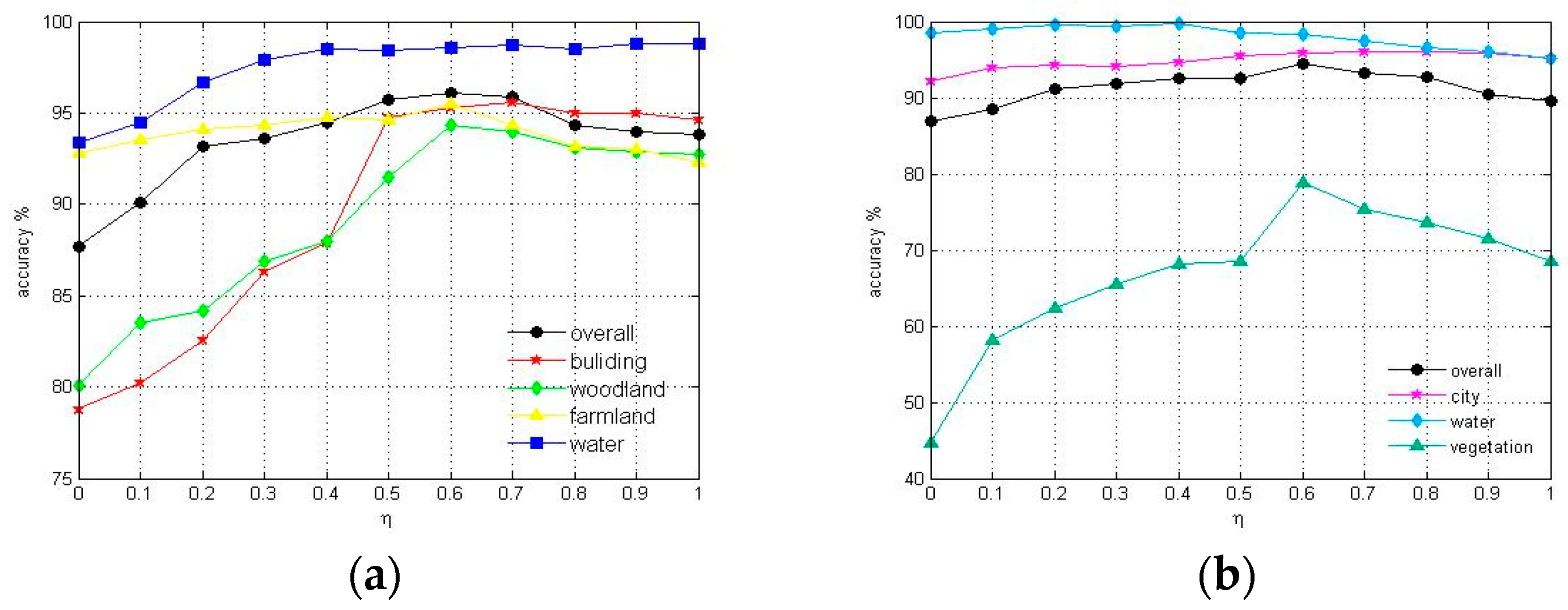
In the training process, the overall accuracy curve in Figure 5a reaches the top when . So, we may conclude that set in Flevoland data set can make the best performance. Similarly, in Figure 5b, setting in San Francisco Bay data set had best outcome. Therefore, we set in the experiment for the Flevoland and San Francisco Bay data sets.
4.3. Results
4.3.1. Flevoland Data Set
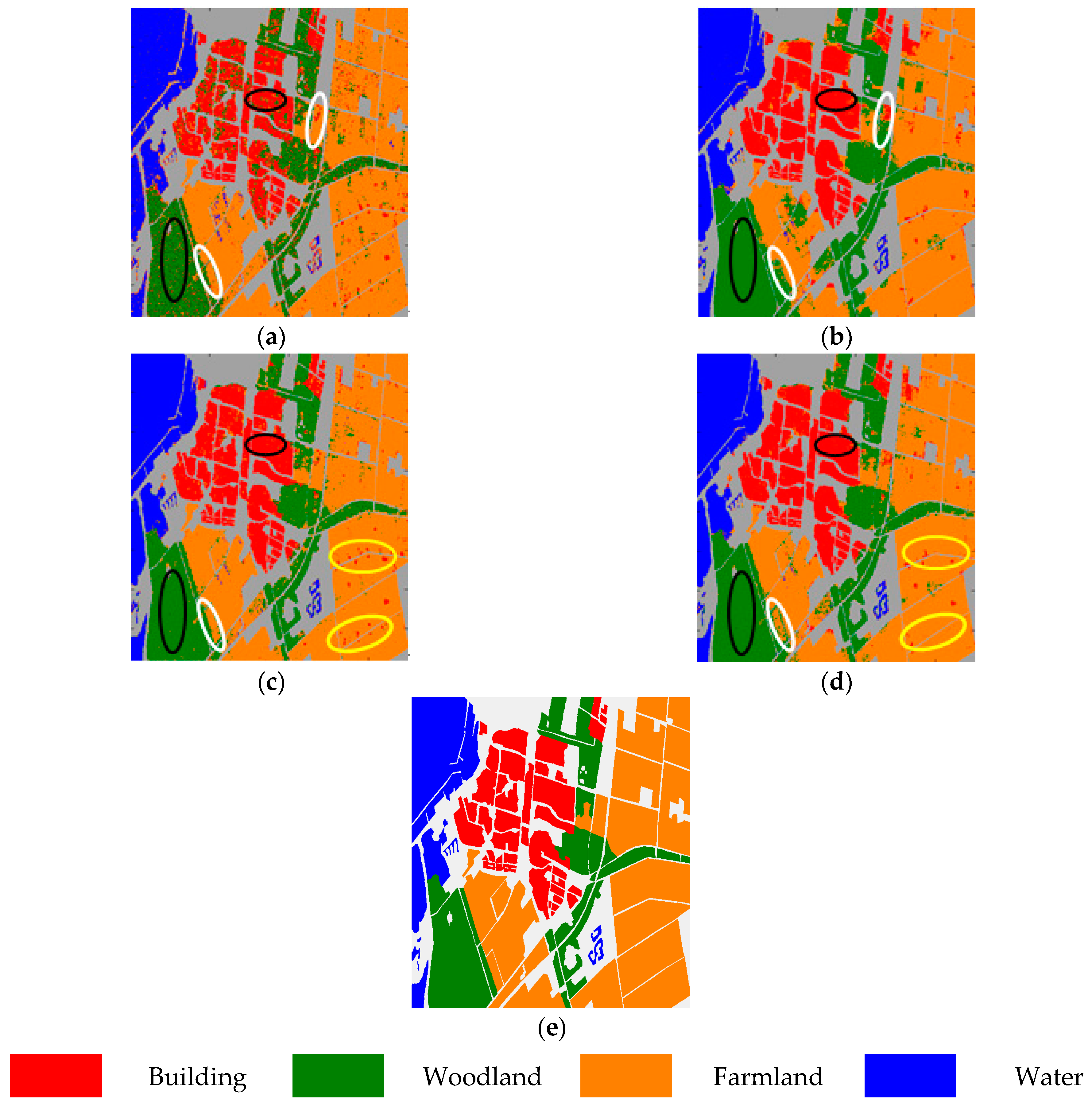
As expected, we can see Figure 6a that, regarding polarimetric features alone, the building area and woodland area in black ellipses show large variation, i.e., pixels of the same land cover type may have very different scattering mechanisms, while pixels of different land cover types may have very similar scattering mechanisms. Moreover, in Figure 6b, morphological features alone may also lead to incorrect classification results, e.g., those two farmland areas in white ellipses that are classified as woodland area. Further, feature fusion via vector stacking also has some flaws; e.g., in Figure 6c, the farmland in yellow ellipses shows obvious variation. However, when combining those two features via composite kernels, the performance of the PolSAR image improves; e.g., in Figure 6d, in black ellipses, building and woodland can be clearly classified, in white ellipses, farmland can be classified, and in yellow ellipses, farmland can also be classified—much better than the vector stacking method. And Figure 6e is the reference map of Flevoland Data Set.
From Table 5, we can see that using polarimetric features alone lead to low accuracy, especially in building areas and woodland areas. Morphological features account for the spatial structural information, which helps to produce more accurate classification results. However, this approach has a slightly low accuracy in farmland area because this approach only considers spatial information. The overall accuracy is distinctly boosted when fusing the two types of information together. The kappa coefficient also notably increases to 0.94. Admittedly, the overall accuracy of vector stacking is similar to that of the composite kernel approach, but it is worth noting that, when the vector stacking method is used, different features should be normalized before stacking. Further, the vector stacking approach does not take the inter-relation of different features into consideration.
4.3.2. San Francisco Bay Data Set
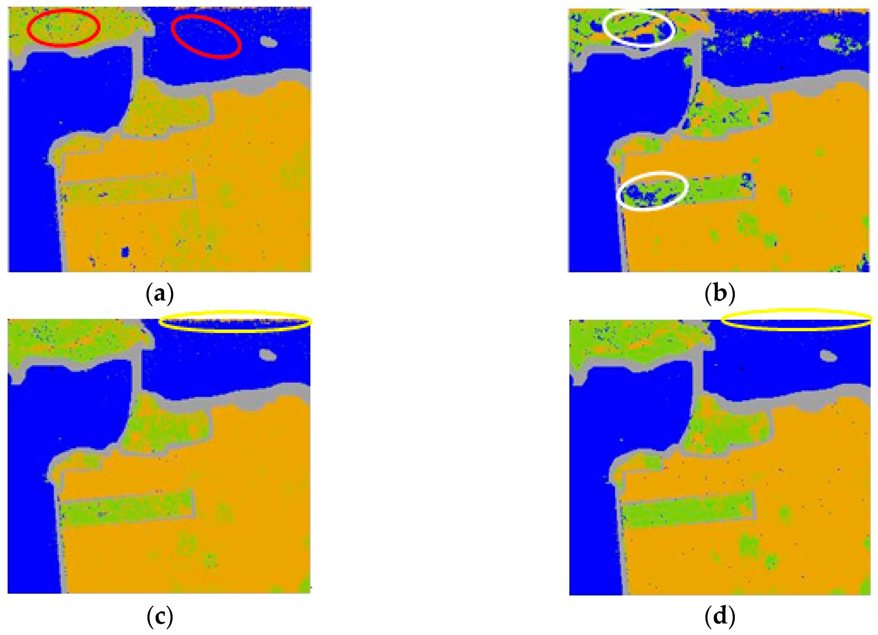
Like the Flevoland data set, firstly, as shown in Figure 7a, the city and water area in red ellipses show large variation. Secondly, in Figure 7b, though morphological features alone show a smoother map, they may also lead to an incorrect classification map, e.g., the two vegetation areas in white ellipses that are classified as water areas. Moreover, feature fusion via vector stacking also has some flaws; e.g., in the upper right (luminous yellow ellipses) of Figure 7c, there are areas and variations that are obviously incorrectly classified. However, when combining those two features via composite kernels, the performance of the PolSAR image improves, and the map of the composite kernel method (in Figure 7d) is smoother and has more correctly classified areas than those of other methods. And Figure 7e is the reference map of San Francisco Bay Data Set.
From Table 6, the overall accuracy of the four methods (only POL, only MP, vector stacking, and composite kernels) is 86.9%, 89.6%, 92.6, and 94.4%, respectively. Compared with the other three methods, the overall accuracy of the new method we proposed is increased by 7%, 4.8%, and 1.8%. The kappa coefficient also exhibits marked growth.
Our results confirm the validation of the composite kernel method. The performance of classification can be boosted when we fuse two types of information. The composite kernel method can tune the contribution of different content, yielding better accuracy than the “stacked” method. However, we have not considered other possible kernel distances. The classification performance may be improved if we take other kernels into account.
5. Conclusions and Future Work
In this paper, a feature fusion approach that exploits both polarimetric and spatial information of PolSAR images is proposed. The polarimetric information is captured by collecting polarimetric signatures. The spatial information is captured by using the morphological transformation. Inspired by the complementarity between spatial and spectral features producing significant improvements in optical image classification, performance can be improved by fusing polarimetric and spatial information in the classifier. Traditionally, the method is based on a “stacked” approach, in which feature vectors are built from the concatenation of polarimetric and spatial features. In this paper, we propose a new method called the “composite kernel” method, which tunes the contribution of different type of features. Compared with one signal feature classification and traditional feature fusion classification via vector stacking, the composite kernel method possesses several excellent properties, making fusion more effective and leading to better performance. The proposed approach has been tested on the Flevoland data set and the San Francisco Bay data set. The obtained results confirm the benefit of combing different types of information via composite kernels for PolSAR image classification.
In the future, we will continue studying PolSAR image classification with polarimetric and spatial features. Other possible kernel distances could be investigated via, for example, the spectral angle mapper. More advanced feature combination methods that solve the problems of feature extraction and combination simultaneously could also be researched. One such framework is multiple kernel learning, which could be utilized as a platform for developing effective classification approaches.
Acknowledgments
This study was supported by the Fundamental Research Funds for the Central Universities A03013023601005 and the National Nature Science Foundation of China under Grant 61271287 and Grant U1433113.
Author Contributions
Zongjie Cao led the study. Xianyuan Wang designed the experimental and wrote the paper. Yao Ding arranged the data sets. Jilan Feng analyzed the data and checked the paper.
Conflicts of Interest
The authors declare no conflict of interest.
References
- Touzi, R.; Boerner, W.M.; Lee, J.S.; Lueneburg, E. A review of polarimetry in the context of synthetic aperture radar: Concepts and information extraction. Can. J. Remote Sens. 2004, 30, 380–407. [Google Scholar] [CrossRef]
- Lee, J.-S.; Pottier, E. Polarimetric Radar Imaging: From Basics to Applications; CRC Press: Boca Raton, FL, USA, 2009. [Google Scholar]
- Doulgeris, A.P.; Anfinsen, S.N.; Eltoft, T. Automated non-Gaussian clustering of polarimetric synthetic aperture radar images. IEEE Trans. Geosci. Remote Sens. 2001, 49, 3665–3676. [Google Scholar] [CrossRef]
- Liu, H.-Y.; Wang, S.; Wang, R.-F. A framework for classification of urban areas using polarimetric SAR images integrating color features and statistical model. J. Infrared Millim. Waves 2016, 35, 398–406. [Google Scholar]
- Fan, K.T.; Chen, Y.S.; Lin, C.W. Identification of rice paddy fields from multitemporal polarimetric SAR images by scattering matrix decomposition. In Proceedings of the IEEE International Symposium on Geoscience and Remote Sensing IGARSS, Milan, Italy, 26–31 July 2015; pp. 3199–3202. [Google Scholar]
- Cloude, S.R.; Pottier, E. A review of target decomposition theorems in radar polarimetry. IEEE Trans. Geosci. Remote Sens. 1996, 34, 498–518. [Google Scholar] [CrossRef]
- Yuan, H.; Tang, Y.Y. Spectral-Spatial Shared Linear Regression for Hyperspectral Image Classification. IEEE Trans. Cybern. 2017, 47, 934–945. [Google Scholar] [CrossRef] [PubMed]
- Zou, T.; Yang, W.; Dai, D.; Sun, H. Polarimetric SAR Image Classification Using Multifeatures Combination and Extremely Randomized Clustering Forests. EURASIP J. Adv. Signal Process. 2010, 2010, 4. [Google Scholar] [CrossRef]
- Tu, S.T.; Chen, J.Y.; Yang, W.; Sun, H. Laplacian eigenmaps based polarimetric dimensionality reduction for SAR image classification. IEEE Trans. Geosci. Remote Sens. 2012, 50, 170–179. [Google Scholar] [CrossRef]
- Shi, L.; Zhang, L.; Yang, J. Supervised graph embedding for polarimetric SAR image classification. IEEE Geosci. Remote Sens. Lett. 2013, 10, 216–220. [Google Scholar] [CrossRef]
- Li, J.; Bioucas-Dias, J.M.; Plaza, A. Spectral-spatial hyperspectral image segmentation using subspace multinomial logistic regression and Markov random fields. IEEE Trans. Geosci. Remote Sens. 2012, 50, 809–823. [Google Scholar] [CrossRef]
- Moser, G.; Serpico, S.; Benediktsson, J.A. Land-cover mapping by Markov modeling of spatial–contextual information in very-high-resolution remote sensing images. Proc. IEEE 2013, 101, 631–651. [Google Scholar] [CrossRef]
- Chen, X.; Fang, T.; Huo, H.; Li, D. Graph-based feature selection for object-oriented classification in VHR airborne imagery. IEEE Trans. Geosci. Remote Sens. 2011, 49, 353–365. [Google Scholar] [CrossRef]
- Liu, B.; Hu, H.; Wang, H.; Wang, K.; Liu, X.; Yu, W. Superpixel-based classification with an adaptive number of classes for polarimetric SAR images. IEEE Trans. Geosci. Remote Sens. 2013, 51, 907–924. [Google Scholar] [CrossRef]
- Dai, D.; Yang, W.; Sun, H. Multilevel local pattern histogram for SAR image classification. IEEE Geosci. Remote Sens. Lett. 2011, 8, 225–229. [Google Scholar] [CrossRef]
- Shen, L.; Zhu, Z.; Jia, S.; Zhu, J.; Sun, Y. Discriminative Gabor feature selection for hyperspectral image classification. IEEE Geosci. Remote Sens. Lett. 2013, 10, 29–34. [Google Scholar] [CrossRef]
- Huang, X.; Zhang, L. An SVM ensemble approach combining spectral, structural, and semantic features for the classification of high-resolution remotely sensed imagery. IEEE Trans. Geosci. Remote Sens. 2013, 51, 257–272. [Google Scholar] [CrossRef]
- Soille, P. Morphological Image Analysis; Springer: Berlin, Germany, 2004. [Google Scholar]
- Devis, T.; Frederic, R.; Alexei, P.; Camps-Valls, G. Composite kernels for Urban-image classification. IEEE Geosci. Remote Sens. Lett. 2010, 7, 88–92. [Google Scholar]
- Du, P.; Samat, A.; Waskec, B.; Liu, S.; Li, Z. Random Forest and Rotation Forest for fully polarized SAR image classification using polarimetric and spatial features. ISPRS J. Photogramm. Remote Sens. 2015, 105, 38–53. [Google Scholar] [CrossRef]
- Molinier, M.; Laaksonen, J.; Rauste, Y.; Häme, T. Detecting changes in polarimetric SAR data with content-based image retrieval. In Proceedings of the IEEE International Geoscience and Remote Sensing Symposium, Barcelona, Spain, 23–28 July 2007; pp. 2390–2393. [Google Scholar]
- Krogager, E. New decomposition of the radar target scattering matrix. Electron. Lett. 1990, 26, 1525–1527. [Google Scholar] [CrossRef]
- Cloude, S.R.; Pottier, E. An entropy based classification scheme for land applications of polarimetric SAR. IEEE Trans. Geosci. Remote Sens. 1997, 35, 68–78. [Google Scholar] [CrossRef]
- Yamaguchi, Y.; Moriyama, T.; Ishido, M.; Yamada, H. Four component scattering model for polarimetric SAR image decomposition. IEEE Trans. Geosci. Remote Sens. 2005, 43, 1699–1706. [Google Scholar] [CrossRef]
- Freeman, A.; Durden, S.L. A three-component scattering model for polarimetric SAR data. IEEE Trans. Geosci. Remote Sens. 1998, 36, 963–973. [Google Scholar] [CrossRef]
- Soille, P.; Pesaresi, M. Advances in mathematical morphology applied to geoscience and remote sensing. IEEE Trans. Geosci. Remote Sens. 2002, 40, 2042–2055. [Google Scholar] [CrossRef]
- Fauvel, M.; Benediktsson, J.A.; Chanussot, J.; Sveinsson, J.R. Spectral and spatial classification of hyperspectral data using SVMs and morphological profiles. IEEE Trans. Geosci. Remote Sens. 2008, 46, 3804–3814. [Google Scholar] [CrossRef]
- Zhao, Y.-Q.; Liu, J.-X.; Liu, J. Medical image segmentation based on morphological reconstruction operation. Comput. Eng. Appl. 2007, 43, 228–240. [Google Scholar]
- Plaza, A.; Martinez, P.; Plaza, J.; Perez, R. Dimensionality reduction and classification of hyperspectral image data using sequences of extended morphological transformations. IEEE Trans. Geosci. Remote Sens. 2005, 43, 466–479. [Google Scholar] [CrossRef]
- Camps-Valls, G.; Gomez-Chova, L.; Muñoz-Mari, J.; Vila-Frances, J.; Calpe-Maravilla, J. Composite kernels for hyperspectral image classification. IEEE Geosci. Remote Sens. Lett. 2006, 3, 93–97. [Google Scholar] [CrossRef]
- Vapnik, V.N. The Nature of Statistical Learning Theory, 2nd ed.; Springer: New York, NY, USA, 2000. [Google Scholar]
- Burges, C. A tutorial on support vector machines for pattern recognition. Data Min. Knowl. Discov. 1998, 2, 121–167. [Google Scholar] [CrossRef]
- Gu, B.; Sheng, V.S. A Robust Regularization Path Algorithm for ν-Support Vector Classification. IEEE Trans. Neural Netw. Learn. Syst. 2016, 28, 1241–1248. [Google Scholar] [CrossRef] [PubMed]
- Gu, B.; Sheng, V.S.; Tay, K.Y.; Romano, W.; Li, S. Incremental Support Vector Learning for Ordinal Regression. IEEE Trans. Neural Netw. Learn. Syst. 2015, 26, 1403–1416. [Google Scholar] [CrossRef] [PubMed]
- Kim, E. Every You Wanted to Know about the Kernel Trick (But Were Too Afraid to Ask). Available online: http://www.eric-kim.net/eric-kim-net/posts/1/kernel_trick.html (accessed on 1 June 2016).
- Gu, B.; Sheng, V.S.; Wang, Z.; Ho, D.; Osman, S.; Li, S. Incremental learning for ν-Support Vector Regression. Neural Netw. 2015, 67, 140–150. [Google Scholar] [CrossRef] [PubMed]
- LIBSVM Tools. Available online: http://www.csie.ntu.edu.tw/~cjlin/libsvmtools (accessed on 1 June 2016).
- Mercer’s Theorem. Available online: https://en.wikipedia.org/wiki/Mercer%27s_theorem (accessed on 1 June 2016).
- Tuia, D.; Ratle, F.; Pozdnoukhov, A.; Camps-valls, G. Multisource composite kernels for urban-image classification. IEEE Geosci. Remote Sens. Lett. 2010, 7, 88–92. [Google Scholar] [CrossRef]
- Kappa Coefficients: A Critical Appraisal. Available online: http://john-uebersax.com/stat/kappa.htm (accessed on 1 June 2016).
Figure 1.
The scheme for polarimetric and spatial feature space construction in polarimetric synthetic aperture radar (PolSAR) images. The polarimetric features are concerned with the ground scattering property at a single pixel, while the spatial features are concerned with the relationship between neighboring pixels by using structural elements with different shapes and sizes.
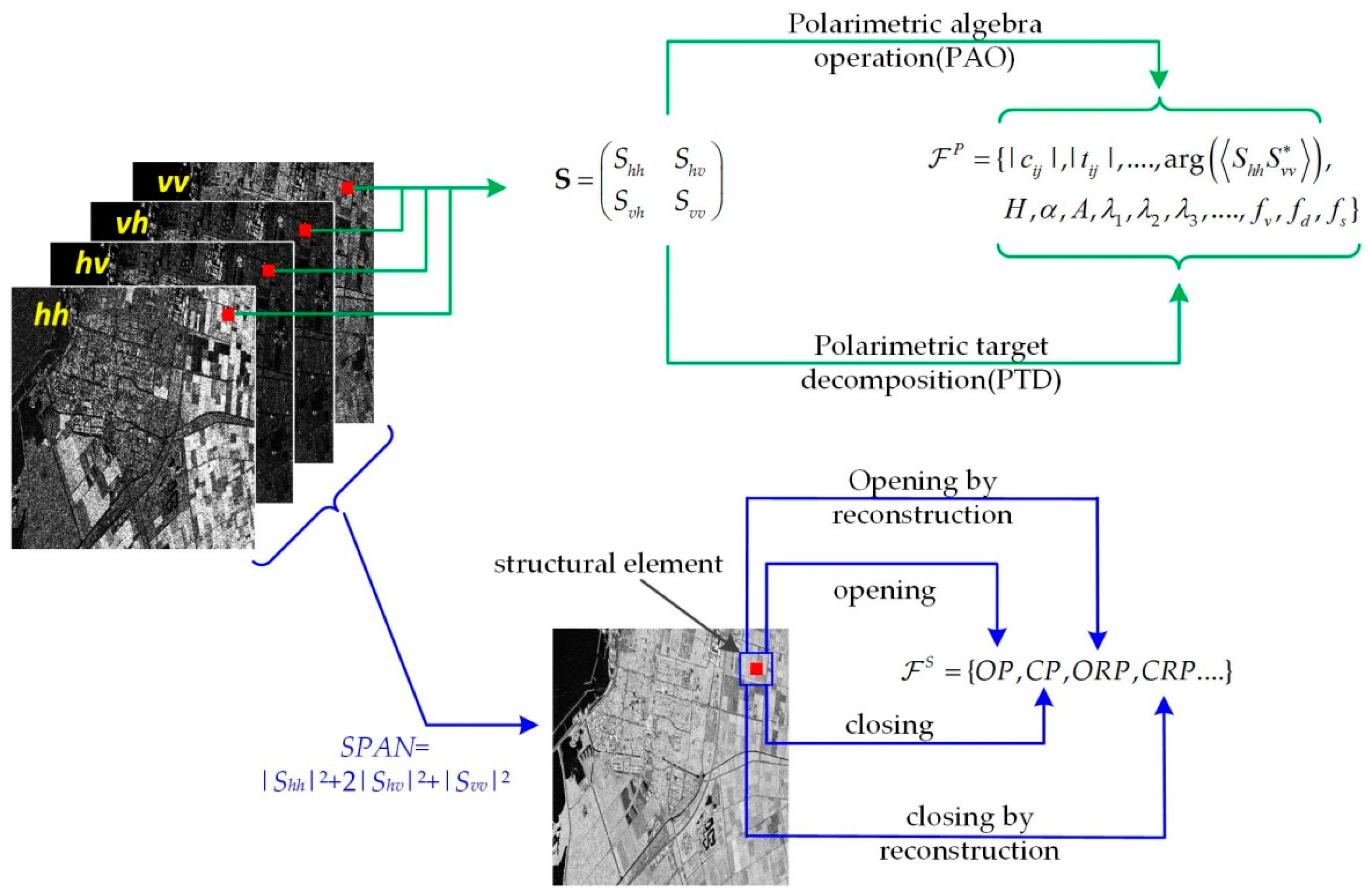
Figure 2.
Polarimetric-spatial classification of PolSAR images by feature fusion.
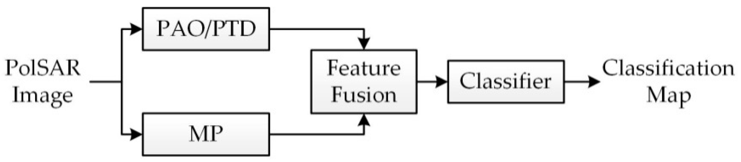
Figure 3.
Flevoland data set collected by RadarSat-2. (a) RGB image obtained by Pauli decomposition. (b) Reference map. A total of four classes are identified. Color-coded class label: red—building area, green—woodland, orange—farmland, and blue—water.
Figure 3.
Flevoland data set collected by RadarSat-2. (a) RGB image obtained by Pauli decomposition. (b) Reference map. A total of four classes are identified. Color-coded class label: red—building area, green—woodland, orange—farmland, and blue—water.
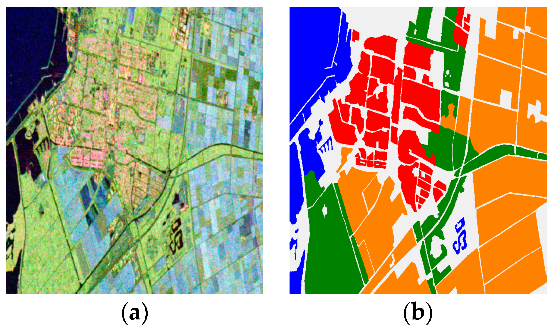
Figure 4.
San Francisco Bay data set collected by AIRSAR system. (a) RGB image obtained by Pauli decomposition. (b) Reference map. A total of three classes are identified. Color-coded class label: yellow—city area, blue—water, and green—vegetation.
Figure 4.
San Francisco Bay data set collected by AIRSAR system. (a) RGB image obtained by Pauli decomposition. (b) Reference map. A total of three classes are identified. Color-coded class label: yellow—city area, blue—water, and green—vegetation.
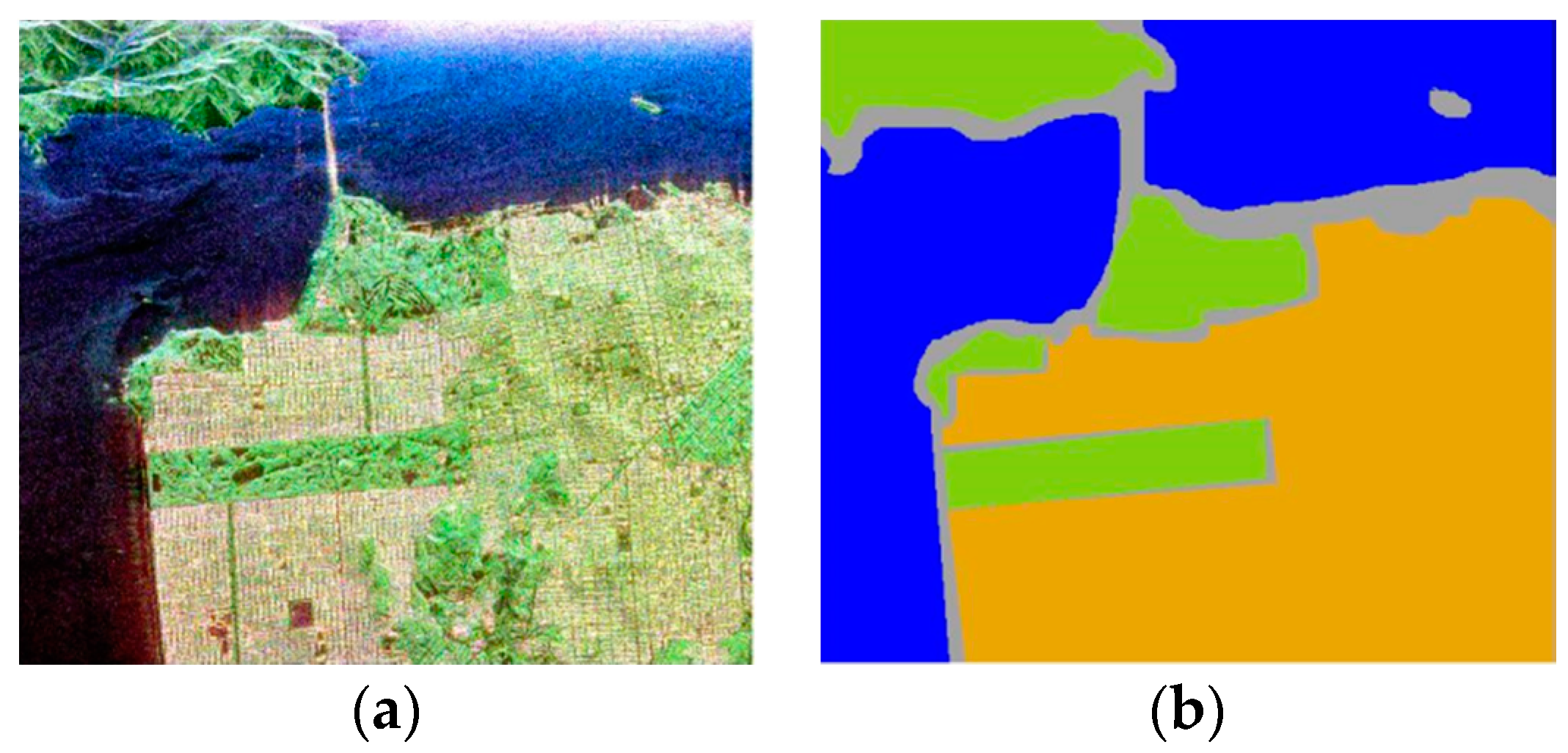
Figure 5.
Accuracy versus weight for Flevoland data set (a) and San Francisco Bay data set (b).

Figure 6.
Classification maps of Flevoland data with different methods. (a) Only polarimetric features. (b) Only morphological features. (c) Feature fusion via vector stacking. (d) Feature fusion via composite kernels. (e) Reference map.
Figure 6.
Classification maps of Flevoland data with different methods. (a) Only polarimetric features. (b) Only morphological features. (c) Feature fusion via vector stacking. (d) Feature fusion via composite kernels. (e) Reference map.

Figure 7.
Classification maps of the San Francisco Bay data set with different methods. (a) Only polarimetric features. (b) Only morphological features. (c) Feature fusion via vector stacking. (d) Feature fusion via composite kernels. (e) Reference map.
Figure 7.
Classification maps of the San Francisco Bay data set with different methods. (a) Only polarimetric features. (b) Only morphological features. (c) Feature fusion via vector stacking. (d) Feature fusion via composite kernels. (e) Reference map.


Table 1.
Summarization of polarimetric signatures considered in this paper.
| Polarimetric Signatures | Expression |
|---|---|
| Amplitude of upper triangle matrix elements of C | |
| Amplitude of upper triangle matrix elements of T | |
| Ratio between HV and HH backscattering coefficient | |
| Ratio between VV and HH backscattering coefficient | |
| Ratio between HV and VV backscattering coefficient | |
| Depolarization ratio | |
| Phase difference HH-VV | |
| Entropy, alpha angle, anisotropy and eigenvalues in Cloude Decomposition | |
| nine parameters of the Huynen Decomposition | |
| Power of surface, double-bounce, volume and helix scatter components in Yamaguchi Decomposition | |
| Coefficient for the volume, double bounce and surface components in Van Zyl Decomposition |
Table 2.
Summarization of morphological operations.
| Morphological Operations | Expression |
|---|---|
| Erosion | |
| Dilation | |
| Opening | |
| Closing | |
| Opening by reconstruction | |
| Closing by reconstruction |
and represent erosion and dilation operation, respectively. and represent SE of dilation and erosion. I represent the SPAN image.
Table 3.
Number of samples of the Flevoland data set used for quantitative evaluation.
| Class | Building | Woodland | Farmland | Water |
|---|---|---|---|---|
| Number of Samples in the Reference Map | 71,331 | 85,539 | 184,920 | 59,504 |
| Number of Training Samples | 713 | 855 | 1849 | 595 |
| Number of Testing Samples | 70,618 | 84,684 | 183,071 | 58,909 |
Table 4.
Number of samples of the San Francisco Bay data set used for quantitative evaluation.
| Class | City Area | Water | Vegetation |
|---|---|---|---|
| Number of Samples in the Reference Map | 391,407 | 315,320 | 135,508 |
| Number of Training Samples | 3914 | 3153 | 1355 |
| Number of Testing Samples | 387,439 | 312,167 | 134,153 |
Table 5.
Classification accuracy measures on the Flevoland data set. The best performance in each column is shown in bold.
Table 5.
Classification accuracy measures on the Flevoland data set. The best performance in each column is shown in bold.
| Method | Building (%) | Woodland (%) | Farmland (%) | Water (%) | Overall Accuracy (%) | Kappa Coefficient |
|---|---|---|---|---|---|---|
| Only POL | 78.8 | 80.1 | 92.8 | 93.4 | 87.7 | 0.842 |
| Only MP | 94.6 | 92.7 | 92.3 | 98.9 | 93.8 | 0.909 |
| Vector Stacking | 95.2 | 93.7 | 96.2 | 97.4 | 95.7 | 0.920 |
| Composite Kernel | 95.6 | 94.3 | 96.2 | 98.8 | 96.1 | 0.942 |
Kappa Coefficient measures the percentage of data values in the main diagonal of the table and then adjusts these values for the amount of agreement that could be expected due to chance alone [40].
Table 6.
Classification accuracy measures on San Francisco Bay data set. The best performances in each column are shown in bold.
Table 6.
Classification accuracy measures on San Francisco Bay data set. The best performances in each column are shown in bold.
| Method | City Area (%) | Water (%) | Vegetation (%) | Overall Accuracy (%) | Kappa Coefficient |
|---|---|---|---|---|---|
| Only POL | 92.2 | 98.5 | 44.7 | 86.9 | 0.783 |
| Only MP | 95.1 | 95.2 | 60.7 | 89.6 | 0.830 |
| Vector Stacking | 96.0 | 98.5 | 68.5 | 92.6 | 0.879 |
| Composite Kernel | 96.0 | 99.7 | 78.8 | 94.4 | 0.909 |
© 2017 by the authors. Licensee MDPI, Basel, Switzerland. This article is an open access article distributed under the terms and conditions of the Creative Commons Attribution (CC BY) license (http://creativecommons.org/licenses/by/4.0/).
Share and Cite
MDPI and ACS Style
Wang, X.; Cao, Z.; Ding, Y.; Feng, J. Composite Kernel Method for PolSAR Image Classification Based on Polarimetric-Spatial Information. Appl. Sci. 2017, 7, 612. https://doi.org/10.3390/app7060612
AMA Style
Wang X, Cao Z, Ding Y, Feng J. Composite Kernel Method for PolSAR Image Classification Based on Polarimetric-Spatial Information. Applied Sciences. 2017; 7(6):612. https://doi.org/10.3390/app7060612
Chicago/Turabian StyleWang, Xianyuan, Zongjie Cao, Yao Ding, and Jilan Feng. 2017. "Composite Kernel Method for PolSAR Image Classification Based on Polarimetric-Spatial Information" Applied Sciences 7, no. 6: 612. https://doi.org/10.3390/app7060612
Note that from the first issue of 2016, this journal uses article numbers instead of page numbers. See further details here.