Article

Application of Matched-Filter Concepts to Unbiased Selection of Data in Pump-Probe Experiments with Free Electron Lasers

by
Carlo Callegari
1,2,*,†,
Tsukasa Takanashi
3,†,
Hironobu Fukuzawa
3,
Koji Motomura
3,‡,
Denys Iablonskyi
3,
Yoshiaki Kumagai
3,§,
Subhendu Mondal
3,
Tetsuya Tachibana
3,
Kiyonobu Nagaya
4,
Toshiyuki Nishiyama
4,
Kenji Matsunami
4,
Per Johnsson
5,
Paolo Piseri
6,
Giuseppe Sansone
7,8,
Antoine Dubrouil
7,‖,
Maurizio Reduzzi
7,
Paolo Carpeggiani
7,
Caterina Vozzi
7,
Michele Devetta
7,
Davide Faccialà
7,
Francesca Calegari
7,9,
Mattea Carmen Castrovilli
7,
Marcello Coreno
1,2,
Michele Alagia
10,
Bernd Schütte
11,
Nora Berrah
12,
Oksana Plekan
1,
Paola Finetti
1,
Eugenio Ferrari
1,¶,
Kevin Charles Prince
1,10 and
Kiyoshi Ueda
3
add Show full author list remove Hide full author list
1
Elettra-Sincrotrone Trieste S.C.p.A., Strada Statale 14–km 163.5 in Area Science Park, 34149 Basovizza, Trieste, Italy
2
CNR-ISM, Area Science Park, 34149 Basovizza, Trieste, Italy
3
Institute of Multidisciplinary Research for Advanced Materials, Tohoku University, Sendai 980-8577, Japan
4
Department of Physics, Graduate School of Science, Kyoto University, Kyoto 606-8502, Japan
5
Department of Physics, Lund University, P.O. Box 118, 22100 Lund, Sweden
6
CIMAINA and Dipartimento di Fisica, Università degli Studi di Milano, Via Celoria 16, 20133 Milano, Italy
7
CNR-IFN, Piazza Leonardo da Vinci 32, 20133 Milano, Italy
8
Physikalisches Institut, Albert-Ludwigs-Universität, 79104 Freiburg, Germany
9
Center for Free-Electron Laser Science, DESY, Notkestrasse 85, 22607 Hamburg, Germany
10
CNR-IOM, Area Science Park, 34149 Basovizza, Trieste, Italy
11
Max-Born-Institut, Max-Born-Strasse 2 A, 12489 Berlin, Germany
12
Department of Physics, University of Connecticut, 2152 Hillside Road, Storrs, CT 06269, USA
*
Author to whom correspondence should be addressed.
These authors contributed equally to this work.
Current address: RIKEN SPring-8 Center, Kouto, Sayo, Hyogo 679-5148, Japan.
§
Current address: Argonne National Laboratory, 9700 S. Cass Avenue, Argonne, IL 60439, USA.
Current address: Femto Easy, Parc scientifique Laseris 1, 33114 Le Barp, France.
Current address: Particle Accelerator Physics Laboratory, École Polytechnique Fédérale de Lausanne EPFL, CH-1015 Lausanne, Switzerland.
Appl. Sci. 2017, 7(6), 621; https://doi.org/10.3390/app7060621
Submission received: 27 April 2017 / Revised: 6 June 2017 / Accepted: 9 June 2017 / Published: 16 June 2017
(This article belongs to the Special Issue X-Ray Free-Electron Laser)

Abstract

:
Pump-probe experiments are commonly used at Free Electron Lasers (FEL) to elucidate the femtosecond dynamics of atoms, molecules, clusters, liquids and solids. Maximizing the signal-to-noise ratio of the measurements is often a primary need of the experiment, and the aggregation of repeated, rapid, scans of the pump-probe delay is preferable to a single long-lasting scan. The limited availability of beamtime makes it impractical to repeat measurements indiscriminately, and the large, rapid flow of single-shot data that need to be processed and aggregated into a dataset, makes it difficult to assess the quality of a measurement in real time. In post-analysis it is then necessary to devise unbiased criteria to select or reject datasets, and to assign the weight with which they enter the analysis. One such case was the measurement of the lifetime of Intermolecular Coulombic Decay in the weakly-bound neon dimer. We report on the method we used to accomplish this goal for the pump-probe delay scans that constitute the core of the measurement; namely we report on the use of simple auto- and cross-correlation techniques based on the general concept of “matched filter”. We are able to unambiguously assess the signal-to-noise ratio (SNR) of each scan, which then becomes the weight with which a scan enters the average of multiple scans. We also observe a clear gap in the values of SNR, and we discard all the scans below a SNR of 0.45. We are able to generate an average delay scan profile, suitable for further analysis: in our previous work we used it for comparison with theory. Here we argue that the method is sufficiently simple and devoid of human action to be applicable not only in post-analysis, but also for the real-time assessment of the quality of a dataset.

1. Introduction

Recently we described the results of a pump-probe experiment, in which the lifetimes of doubly excited states of neon dimers were measured [1]. The dimers were excited by absorption of two EUV photons from the Free Electron Laser (FEL) FERMI-1 [2] and probed via ionization by a UV laser pulse.
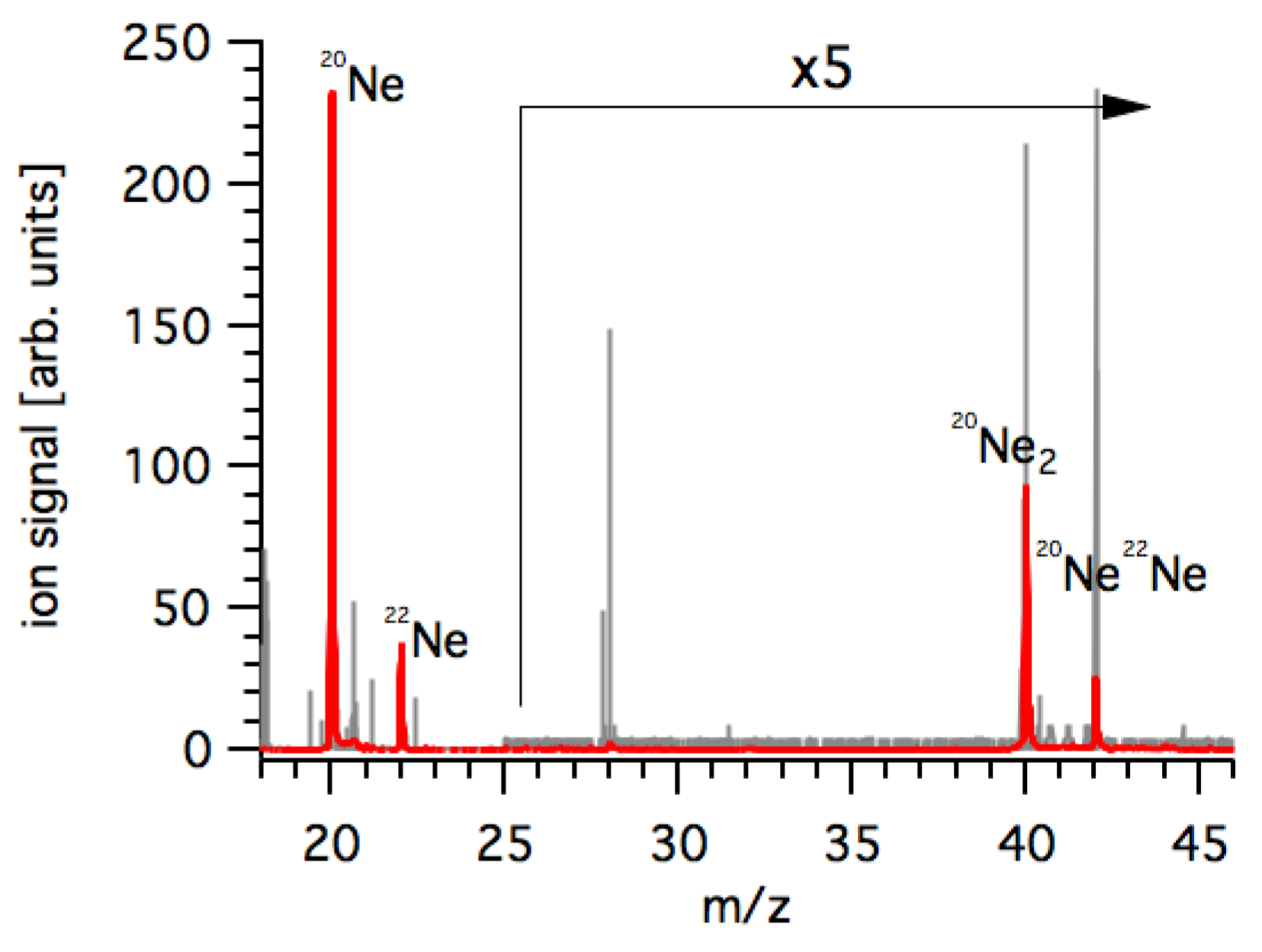
The excited dimers decayed by Interatomic Coulombic Decay to stable dimer cations Ne 2 + , which were detected by a time-of-flight (TOF) mass spectrometer. Ionization by the UV pulse led to a repulsive state of the dimer, which dissociated, so that the yield of dimer ions was reduced, and the yield of Ne + increased. The dimer sample used in that work was very dilute with a large atomic background, as it was produced in a supersonic expansion of neon gas, with a yield of about 1%. The data were therefore noisy, and a substantial effort was needed to analyze and filter them. In this paper, we describe the methods used for that analysis.
The data consisted of a number of temporal scans, each lasting approximately 30 min, in which the ion-TOF signal was measured as a function of the delay between pump and probe pulses, and these scans had poor signal-to-noise ratios. Simply averaging them did not give good results, probably because some of them suffered from poor FEL conditions or poor alignment of the pump and probe pulses. One should reject those scans that do not contribute significant signal, while avoiding human bias. A possible approach is to exploit the difference between signal and noise with respect to auto- and cross-correlation. This is an instance of the more general concept of “matched filter”, i.e., the linear filter maximizing the signal-to-noise ratio (SNR) of a measured noisy sample [3]. Under the assumption of white noise, the matched filter is the complex-conjugate time-reversal of the signal sought, i.e., application of the matched filter returns the autocorrelation of the signal [4]. The concept is widely applied in signal processing, where one is primarily interested in extracting a burst of periodic signal from a noisy sample. As far as peak detection is concerned, a popular field of application is chromatography, but the general results obtained there apply equally well to our case; Ref. [5] explicitly discusses the use of a matched filter to determine amplitude and time shift of the peak being sought. We consider the use of auto- and cross-correlation for three purposes:
  • validate the scans to be included or excluded from averaging
  • determine the weight with which each scan should enter the average
  • determine, if desired, by how much to temporally shift a scan prior to averaging

2. Results

For a set of delays { d i } , i = 0 . . n , let us consider two delay scans R = { R 0 , , R n } and S = { S 0 , , S n } each consisting of a sequence of Ne 2 + ion-TOF signals, reduced as explained in Section 4, and padded with zeros outside of the delay range scanned. We will consider R our reference scan, which for convenience is assumed to be noise-free.
The definition of cross-correlation without normalization, Γ RS , q is:
Γ RS , q = i R i S i + q ( R S ) q
Note that Γ is linear in the two sequences (scaling either one by a factor α scales Γ by the same factor), and that Γ SS , q is the autocorrelation of S , which has a maximum for q = 0 :
( S S ) 0 = i ( S i ) 2
We now assume that any scan N = { N 0 , , N n } consisting of pure noise has zero (negligible) cross-correlation with any other scan (including itself except, obviously, at zero-shift), thus:
( N N ) q = δ q 0 i ( N i ) 2
( R N ) q = 0
with δ q 0 the Kronecker delta; we use Equation (3) to define a variance σ 2 = ( N N ) 0 = i ( N i ) 2 . Equations (3) and (4) strictly hold for white noise and infinite n; in a real-life situation we can expect that noise correlation just decays much faster than signal correlation: thus all scans whose autocorrelation is sharply peaked are probably pure noise, and will also have poor cross-correlation with the reference scan.
Any noisy scan S can be written in terms of the reference scan R and a pure-noise sequence N as: S = α R + N , with α a real number. In a worse-case scenario, S i may be shifted (for simplicity by an integer index r), that is: S i = α R i + r + N i . Then:
( R S ) q = α ( R R ) q r + ( R N ) q = α ( R R ) q r
note that R S is proportional to R R but shifted by r as expected; this is the argument invoked in Ref. [5] to associate the position of the maximum of the cross-correlation function to the shift of the peak being sought. In our work [1] it was not necessary to include a shift; while Equation (5) could be used to estimate the signal amplitude α , it is preferable to use the autocorrelation instead:
( S S ) q = α 2 ( R R ) q + ( N N ) q = α 2 ( R R ) q + σ 2 δ q 0
(note that the shift by r cancels, here). Equation (6) tells us in particular that all autocorrelation sequences should be the same except for a scale factor α 2 and a sharp noise peak at q = 0 
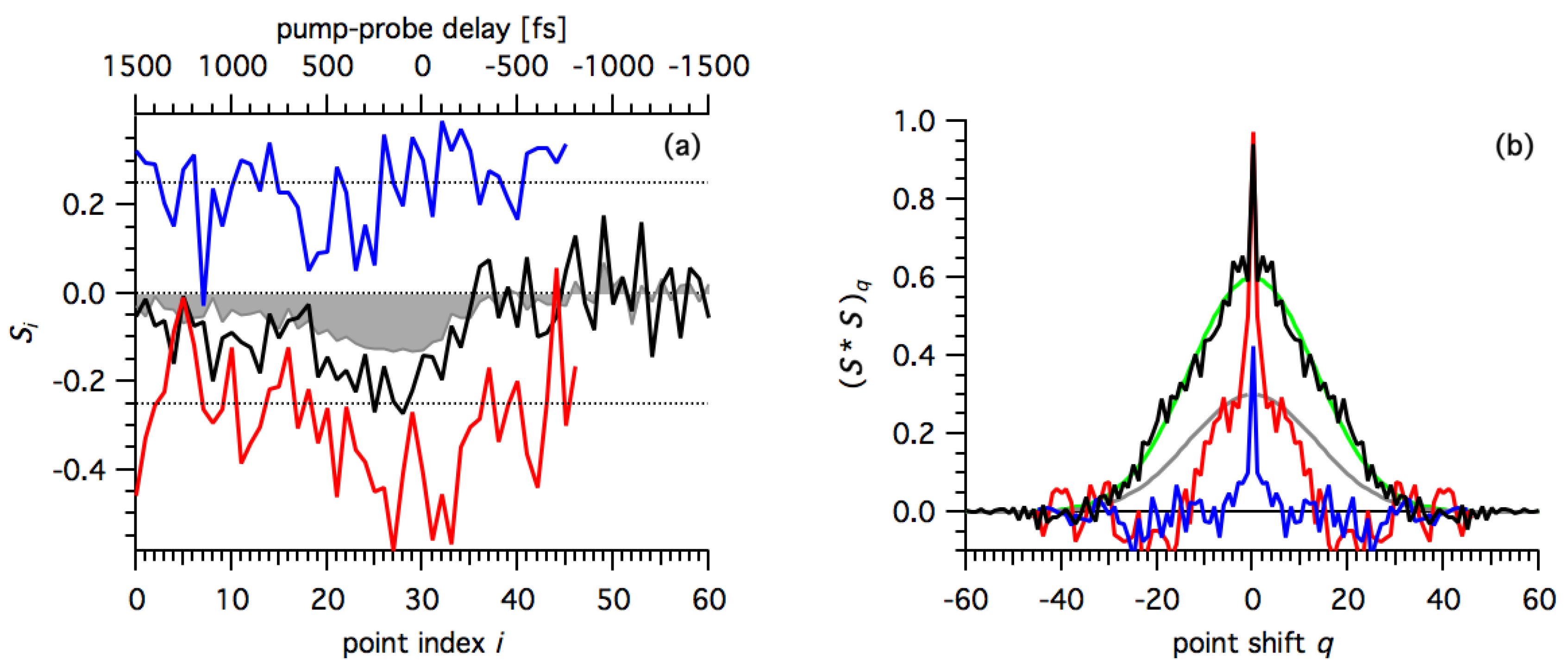
. Visual inspection shows that this is true for a number of scans which we consider good; other scans exhibit a narrower, or structured, sometimes negative, autocorrelation, probably indicating correlated noise, i.e., a drift during the measurement; the rest only exhibits the noise peak, indicating no signal at all (Figure 1). From now on we will consider ( R R ) to be noiseless and, as empirically found, satisfactorily approximated by a gaussian; we derive the width of the gaussian from our best scan (Figure 1).
Our choice of a gaussian is purely empirical, and our method does not critically depend on it: to the extent that all good scans have the same shape of the autocorrelation function, Equation (6), the best fit parameters will be the same for all good scans, except for a scale factor for the height. What is important is that the fitting function provides a reasonable approximation of α in Equation (6), i.e., of the peak value of the signal component of the autocorrelation.
It is nevertheless instructive to discuss some limiting cases for the shape of the autocorrelation function: we begin by noting that the expected shape of a pump-probe signal such as that of our experiment is an exponential decay (we ignore the possible complication brought on by the presence of more than one decay constant) convoluted with the instrumental resolution (in our case a gaussian, coming from the finite duration of the FEL and UV pulses). The respective autocorrelation functions are an exponential and a gaussian. For the case of non-negligible instrumental resolution the autocorrelation will resemble a gaussian near q = 0 , but will have broader wings decaying as exp ( | q | ) rather than exp ( q 2 ) . An early truncation of the scan will clip the wings of the autocorrelation function. In our case an early truncation does somewhat contribute to determining the shape of the autocorrelation function, but does so equally for all scans (the pump-probe delay was scanned in reverse, and point index i = 0 in Figure 1 consistently corresponds to the maximum value of the delay).
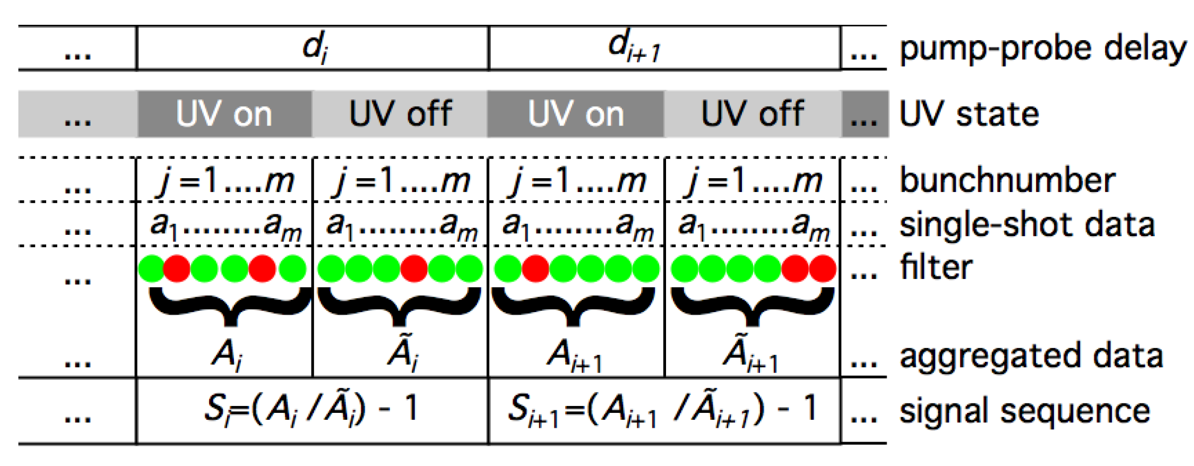
Let us finally consider two possible sources of artefacts, namely a constant, or a linearly drifting, baseline (remembering that the scans are padded with zeros outside of the delay range scanned). This would primarily contribute a slowly decaying component to the autocorrelation signal (of width comparable to that of the scan itself). Let us however note that because the scans are acquired by rapid double-background subtraction (Equation (9) and Figure 4), we expect a complete baseline cancellation. Finally, a drifting signal would alter the shape of the peak and consequently of its autocorrelation function: assuming an even drift that causes a loss of the optimal experimental conditions (temporal or spatial overlap; quality of the focus; resonance wavelength) one can speculate that its main effect would be a reduction of the measured width.

3. Discussion

Given a set of scans S ( k ) , their weighted average is
S = k w k S ( k ) k w k
S is the quantity reported in our work ([1] note for the sake of exactness that in Figure 2a therein, the unity baseline was not subtracted); we want to determine which scans to include in the average, and their weights w k .
From Equation (6) and Figure 1b we can estimate the signal-to-noise ratio as:
SNR k = ( S ( k ) S ( k ) ) 0 ( N ( k ) N ( k ) ) 0 1 = α k 2 ( R R ) 0 ( N ( k ) N ( k ) ) 0 = α k σ k
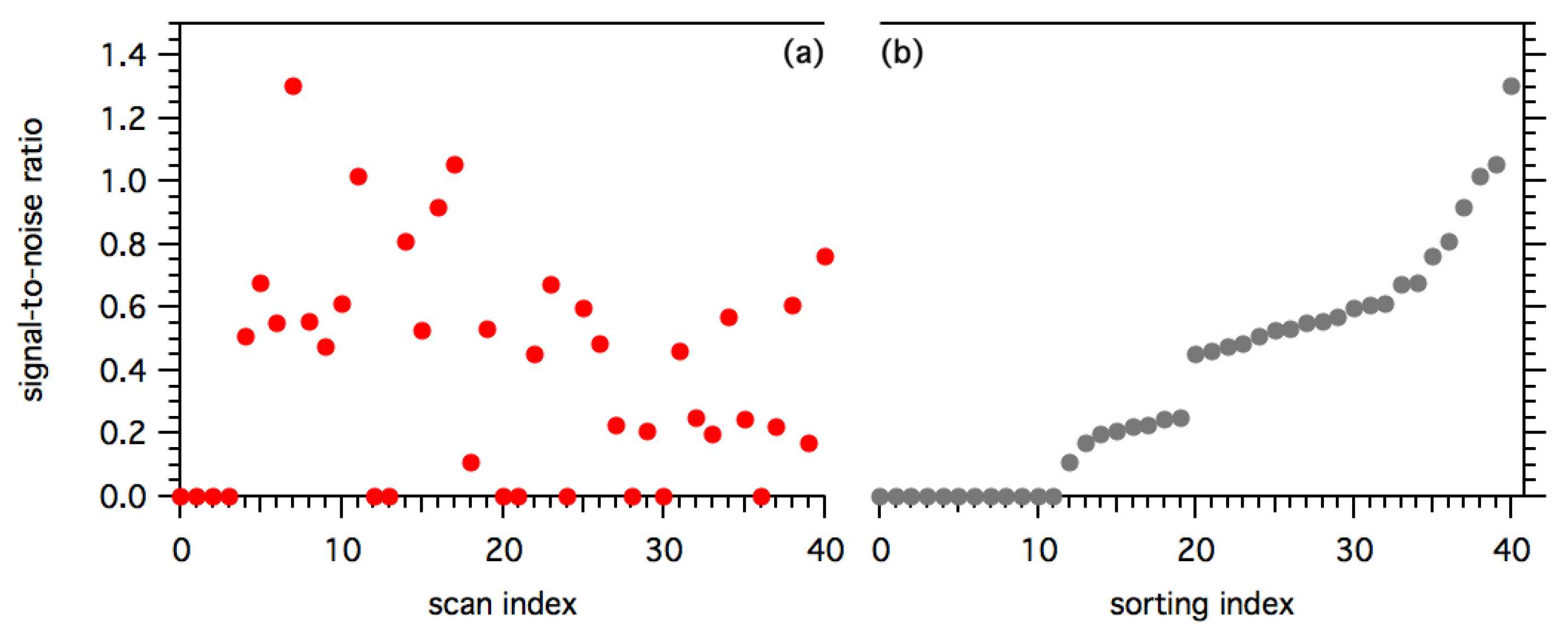
A simple analysis of its trend over the course of the experiment reveals some regularities that we exploit to qualitatively classify scans, and to define a quantitative criterion that we adopt to accept or reject them. When the scans are ordered in the sequence they were acquired (Figure 2a) no obvious trend is visible for the S N R , but one does note a large number of scans with S N R = 0 : they are either those for which a gaussian fit of the autocorrelation was not successful, or those which have been excluded a priori (e.g., because the scan was aborted). The ordering of the scans by increasing SNR (Figure 2b) reveals a gap between scans with SNR < 0.25 and SNR > 0.45 . We cannot find an obvious reason for this gap; because this was one of the first resonant two-photon experiments performed at FERMI we can speculate a threshold behavior of some of the less-controlled parameters of the FEL (peak intensity; second harmonic content). In any case, we decided to use the condition SNR > 0.45 as a discriminant to include a scan in the average.
Let us now come to the weight with which each accepted scan enters the average. We show in Appendix A that the weight which maximizes the SNR of S is w k = α k / σ k 2 = SNR k / σ k ; in Ref. [1] we used w k = SNR k , which gives a slightly worse result, although the difference is not significant. We presume that the latter fact depends on the limited number of samples, the predominance of few of them (see Figure 2a), and the low dispersion of the σ k . In both cases we observe an improvement of the signal-to-noise ratio of S by a factor ≈2.25 relative to the best single scan.
Unfortunately at the time of the experiment we were not anticipating the need for this test, so we are not able to perform further checks on which parameters and events mostly affected our experiment. Likewise our primary goal was to identify a simple unbiased method of data selection, and we do not attempt a systematic analysis of its merits and limitations, for which we refer the reader to the vast existing literature ([6,7] and references therein); we simply note that the method is most easily applicable to the case of white noise and single- or well-separated peaks, although generalizations to other noise [6] or multiple peaks [8] have been discussed. Let us finally note that because the autocorrelation is the Fourier Transform of the power spectrum (Wiener-Khinchin Theorem), the same determination of the signal-to-noise ratio could have been accomplished by Fourier Transform of each scan (in the frequency domain, the white-noise component appears as a constant).
Despite its simplicity and limitations, we believe that our simple test can be further characterized and profitably applied in future experiments. Let us note that the original and most immediate application of the method addresses a situation common to the beginning of many experiments, namely the need of making a weak signal visible when the expected signal shape is not precisely known in advance.

4. Materials and Methods

4.1. Experimental

The experiment was performed at the Low Density Matter (LDM) beamline [9] at FERMI FEL-1 [2]. The EUV pulses had an average energy of 16 μ J, duration estimated between 60 and 80 fs FWHM, circular polarization, focal size 30 μ m FWHM, and were tuned to the wavelength resonant with the two-photon doubly excited target state, 75.65 nm. The UV pulses had an energy of 35 μ J, estimated duration 200 fs, focal size 80 μ m FWHM, fixed wavelength (261 nm). The Ne dimers were produced by adiabatic expansion of Ne gas at a pressure of 0.8 MPa and temperature of 190 K through a 100 μ m nozzle. The target ions were detected by the time-of-flight mass spectrometer of the LDM endstation [10].

4.2. Data Acquisition

The Free Electron Laser FERMI currently operates at a repetition rate of 50 Hz (10 Hz at the time of the experiment). This is determined by the operation rate of the LINAC that accelerates the electron bunches used to generate the FEL pulses. Single-shot ion TOF traces (Figure 3) are acquired, tagged with a progressive integer (“bunchnumber”) and stored along with a wide selection of experimental parameters and machine parameters, for post-processing. The relevant single-shot quantities for us are the FEL energy per pulse ( I 0 ), the UV energy per pulse ( I UV ), and the integrated area a of the TOF peak of interest (specifically the 20 Ne 2 + peak).
A preset number of single-shot values a j at nominally identical conditions are acquired and aggregated into a datapoint A i ; one in three shots is a blank shot (no gas sample), which is subtracted from the average to eliminate spurious signals (Equation (9)). Although in reality the bunchnumber is never reset, i.e., each bunchnumber is unique since the inception of FERMI, for the purpose of this work we will think of it as spanning a range j = { 1 . . m } for each datapoint. A set of datapoints at a sequence of delay values constitutes a delay scan. Delay scans are averaged into a global delay scan, where each scan enters with the weight determined in Equation (8).

4.3. Data Reduction

From the single-shot values we build a datapoint as follows:
A i = j = gas a j j = gas I 0 j p j = blank a j j = blank I 0 j p
with the new index i labelling sets of nominally identical measurements at a series of pump-probe delays d i . A ˜ i is the analogue of A i with UV off. We consider equally spaced delays, so d i = Δ t × i   ( i = 0 . . n ) . Let us note that single-shot data can be excluded from the sum by applying in post-analysis suitable filter conditions (e.g., a threshold on I 0 , or on the quality of the FEL spectrum); for this reason the number of single-shots aggregated into a datapoint is not strictly constant. For each i we define the quantity S i = A i / A ˜ i 1 : this is the base datapoint of a delay scan (Figure 4). The integer p in Equation (9) is the normalization order; for the data presented in Ref. [1] we chose p = 0 , i.e., no normalization. Let us also note that the intensity of the UV pulse was kept constant and is very stable, so it does not appear in the data processing. Let us finally note that at negative delays, and large positive delays we expect the UV to have no effect, i.e., S i = 0 .
Figure 4. Schematic representation of the generation of a delay scan { S i } , as a function of pump-probe delay { d i } from single-shot data a j . The green (red) dots symbolize shots that pass (fail) the filter conditions.
Applsci 07 00621 g004

5. Conclusions

Although rather simple, the method proposed has many advantages and applications. It provides a quick and reliable method to evaluate the quality of a measurement in real time, even when the shape of the expected signal is unknown. In fact, in the approximation of white noise, and of an unstructured pump-probe signal, it provides a first coarse estimate of the signal shape, and thus of the delay range that needs to be scanned. In post-analysis it provides an unbiased criterion to include each scan in an averaged measurement.

Acknowledgments

This work was supported by the X-ray Free Electron Laser Priority Strategy Program of the Ministry of Education, Culture, Sports, Science, and Technology of Japan (MEXT); by JSPS and CNR under the Japan - Italy Research Cooperative Program; by the Grant-in-Aid for the Global COE Program ’the Next Generation of Physics, Spun from Universality and Emergence’ from the MEXT; by the Grants-in-Aid (No. 20310055 and No. 21244062) from the Japan Society for the Promotion of Science (JSPS); by the JSPS KAKENHI Grant Number JP 16J02270; by the Swedish Research Council and the Swedish Foundation for Strategic Research; by the ERC Starting Research Grant UDYNI No. 307964; by the European Union Horizon 2020 research and innovation programme under the Marie Skłodowska-Curie grant agreement No. 641789 “MEDEA” (Molecular Electron Dynamics investigated by IntensE Fields and Attosecond Pulses); by the DOE-SC-BES under Award No. DE-SC0012376; and by the Italian Ministry of Education, Universities and Research (MIUR) (PRIN 2012 - NOXSS)

Author Contributions

K.U. conceived and designed the experiment; A.D., B.S., C.C., C.V., D.F., D.I., E.F., F.C., G.S., H.F., K.C.P., Ke.M., Ko.M., K.N., K.U., M.A., M.C., M.C.C, M.D., M.R., N.B., O.P., P.C., P.F., P.J., P.P., S.M., T.N., Ts.T., Te.T., Y.K. performed the experiments; C.C., H.F., Ko.M., Ts.T. analyzed the data; A.D., C.C., P.J., P.P. contributed analysis tools; C.C. and K.C.P. drafted the paper, which was completed in consultation with all authors.

Conflicts of Interest

The authors declare no conflict of interest. The founding sponsors had no role in the design of the study; in the collection, analyses, or interpretation of data; in the writing of the manuscript, and in the decision to publish the results.

Abbreviations

The following abbreviations are used in this manuscript:
EUVExtreme Ultra Violet
FELFree Electron Laser
FERMIFree Electron laser Radiation for Multidisciplinary Investigations (this acronym identifies the Free Electron Laser facility in Trieste, Italy)
FWHMFull Width at Half Maximum
I0FEL energy per pulse
LINACLinear Particle Accelerator
S N R Signal-to-noise Ratio
TOFTime-of-flight
UVUltra Violet

Appendix A

We demonstrate that within a proportionality factor the optimum value of the weights appearing in Equation (7) is w j = α j σ j 2 ; all three quantities α j , σ j , w j are assumed positive; note that we use j to indicate a specific index, and tacitly replace it with k whenever it becomes a dummy index in a sum. We wish to maximize
k w k α k 2 k w k 2 σ k 2 λ 1 k w k
where λ is a Lagrange multiplier. The condition of zero partial derivatives with respect to each of the w j and of λ yields:
2 a j k w k α k k w k 2 σ k 2 2 w j σ j 2 k w k α k 2 + λ k w k 2 σ k 2 2 = 0
k w k = 1
Multiplying (A2) by w j and summing over j, one has:
2 k w k α k 2 k w k 2 σ k 2 2 k w k 2 σ k 2 k w k α k 2 + λ k w k k w k 2 σ k 2 2 = 0
hence λ = 0 ; and Equation (A2), divided by 2 σ j 2 0 , simplifies to
a j σ j 2 k w k 2 σ k 2 w j k w k α k = 0
Summing over j, and using Equation (A3) yields
k w k α k = k a k σ k 2 k w k 2 σ k 2
which replaced in Equation (A5) finally gives
w j = a j / σ j 2 k a k / σ k 2
Note that in the special case when α k is the same for all k, one has the familiar result that the minimum variance of an average is the one with w j = σ j 2 / k σ k 2 [11].

References

  1. Takanashi, T.; Golubev, N.V.; Callegari, C.; Fukuzawa, H.; Motomura, K.; Iablonskyi, D.; Kumagai, Y.; Mondal, S.; Tachibana, T.; Nagaya, K.; et al. Time-Resolved Measurement of Interatomic Coulombic Decay Induced by Two-Photon Double Excitation of Ne2. Phys. Rev. Lett. 2017, 118, 33202. [Google Scholar] [CrossRef] [PubMed]
  2. Allaria, E.; Appio, R.; Badano, L.; Barletta, W.A.; Bassanese, S.; Biedron, S.G.; Borga, A.; Busetto, E.; Castronovo, D.; Cinquegrana, P.; et al. Highly coherent and stable pulses from the FERMI seeded free-electron laser in the extreme ultraviolet. Nat. Photonics 2012, 6, 699–704. [Google Scholar] [CrossRef]
  3. Green, P. Preface to the matched filter issue. IRE Trans. Inf. Theory 1960, 6, 310. [Google Scholar] [CrossRef]
  4. North, D. An Analysis of the factors which determine signal/noise discrimination in pulsed-carrier systems. Proc. IEEE 1963, 51, 1016–1027. [Google Scholar] [CrossRef]
  5. Van den Heuvel, E.; van Malssen, K.; Smit, H. Optimal estimation of intensity of noisy peaks by matched filtering with application to chromatography. Anal. Chim. Acta 1990, 235, 343–353. [Google Scholar] [CrossRef]
  6. Smit, H. Specification and estimation of noisy analytical signals: Part I. Characterization, time invariant filtering and signal approximation. Chemom. Intell. Lab. Syst. 1990, 8, 15–27. [Google Scholar] [CrossRef]
  7. Smit, H. Specification and estimation of noisy analytical signals: Part II. Curve fitting, optimum filtering and uncertainty determination. Chemom. Intell. Lab. Syst. 1990, 8, 29–41. [Google Scholar] [CrossRef]
  8. Van den Bogaert, B.; Boelens, H.F.M.; Smit, H.C. Quantification of overlapping chromatographic peaks using a matched filter. Chemom. Intell. Lab. Syst. 1994, 25, 297–311. [Google Scholar] [CrossRef]
  9. Svetina, C.; Grazioli, C.; Mahne, N.; Raimondi, L.; Fava, C.; Zangrando, M.; Gerusina, S.; Alagia, M.; Avaldi, L.; Cautero, G.; et al. The Low Density Matter (LDM) beamline at FERMI: optical layout and first commissioning. J. Synchrotron Radiat. 2015, 22, 538–543. [Google Scholar] [CrossRef] [PubMed]
  10. Lyamayev, V.; Ovcharenko, Y.; Katzy, R.; Devetta, M.; Bruder, L.; LaForge, A.; Mudrich, M.; Person, U.; Stienkemeier, F.; Krikunova, M.; et al. A modular end-station for atomic, molecular, and cluster science at the low density matter beamline of FERMI@Elettra. J. Phys. B 2013, 46, 164007. [Google Scholar] [CrossRef]
  11. Bevington, P.R.; Robinson, D.K. Data Reduction and Error Analysis for the Physical Sciences, 2nd ed.; McGraw-Hill: New York, NY, USA, 1992. [Google Scholar]
Figure 1. (a) Three representative delay scans and (b) their autocorrelation curves. We use the autocorrelation curves ( q = 0 excluded) as a criterion to classify scans as good (black), drifting (red), or pure noise (blue). The autocorrelation curve of a good scan is well approximated by a gaussian (green). In panel (a), traces have been offset for clarity, and the shaded curve is the weighed average Equation (7); in panel (b), the green curve is a gaussian fit of the black autocorrelation trace; the gray curve is the same, scaled to the height of the red autocorrelation trace (white-noise peak excluded). The calculated signal-to-noise ratio ( S N R ) for the three scans are 1.30, 0.52, and 0.20.
Applsci 07 00621 g001
Figure 2. (a) Signal-to-noise ratio plotted versus scan index. (b) Same data as (a) sorted by increasing value, to highlight the gap between SNR > 0.25 and SNR < 0.45 .
Applsci 07 00621 g002
Figure 3. Single-shot ion-TOF trace (gray) and average over 12 , 200 shots (red). One in three shots is a blank shot (no gas sample), which is subtracted from the average to eliminate spurious signals, such as that at m / z = 28 in the single shot spectrum, due to residual nitrogen gas. Note that for m / z > 25 both spectra are magnified by a factor 5.
Applsci 07 00621 g003

