
Efficiency Evaluation of Operation Analysis Systems Based on Dynamic Data Envelope Analysis Models from a Big Data Perspective

1
School of Economics and Management, North China Electric Power University, Beijing 102206, China
2
State Grid Energy Research Institute, Beijing 102209, China
3
Department of Economics and Management, Yan’an University, Shanxi 716000, China
4
Deltac Energy Technology Co. Ltd., Beijing 100084, China
*
Author to whom correspondence should be addressed.
Appl. Sci. 2017, 7(6), 624; https://doi.org/10.3390/app7060624
Submission received: 14 April 2017
/
Revised: 12 June 2017
/
Accepted: 12 June 2017
/
Published: 16 June 2017
(This article belongs to the Special Issue Simulation, Analysis, Optimization and New Challenges of District Heating and Cooling Networks)
Abstract
:The operating environment of power grid enterprises is complex with a range of monitoring indicators. To grasp the overall operational status in time and find the key affecting factors, Balanced Scorecard Card (BSC), Interpretive Structural Model (ISM), Principal component analysis (PCA) should be applied. This paper proposed several grid enterprise operators and monitoring indicator systems (which include achievement indicators and driver indicators), and applied PCA for verification and evaluation. The achievement indicators mainly reflected the effectiveness of business operations, which included corporate value, social value, customer value, and so on. Driver indicators mainly reflected the core resources and operations process management of business operations, which have a direct impact on the achievement indicators. The driver and achievement indicators were used as input and output indicators for the provinces to assess the efficiency of operations, and appropriate measures were proposed for improvement. The results showed that the dynamic data envelopment analysis (DEA) model could reflect the time lag of the grid enterprises operating investment and income much better than the other two methods, and the static changes compared to assess efficiency had an average around 4%.
1. Introduction
As distributed energy has developed, regional energy grids have gradually formed. For example, in industrial parks, the Combined Cooling Heating and Power (CCHP), which has formed a network structure of district energy power generation, heating, and cooling, has been adopted. Energy efficiency has been improving with the development of distributed energy, but has also brought new challenges to district heating and cooling networks, especially for district power grid operation and management, which calls for greater requirements. Enterprise operational efficiency evaluation is an important method used to evaluate the investment behavior and effectiveness of managers. An efficiency evaluation of power grid enterprises is mainly conducted to evaluate the efficiency of grid investment behavior made by power grid enterprise managers, and to sort the evaluation object based on the evaluation results to provide the theoretical basis for judging the investment behavior of power grid enterprises.
First, a grid operational efficiency evaluation should involve both design and management issues, which are inseparable. At present, however, evaluations of the operating efficiency of power grid enterprises mainly focus on financial indicators, and ignore the entire process of operations management, which leads to some existing problems of evaluation as the evaluation method is limited to the feasibility study of the single power grid construction project, and the non-financial indicators are always despised. Furthermore, these types of evaluation mainly use the financial internal rate of return and financial net present value to reflect the performance of a single power grid construction project, so lack indicators that can accurately reflect supply reliability, voltage, and cannot completely reflect power grid development and efficiency. Therefore, this paper puts forward the analysis of operational performance indicators based on the whole process of grid operation perspective, extracts key indicators through scientific and reasonable methods, and uses them as input–output indicators to analyze the efficiency of the assessment objects.
Second, a proposal has been made for the use of the Cobb Douglas production function as an intelligent technology evaluation method in the analysis of the technical progress of a grid. This method reflects the development level of an intelligent power grid through the contribution of technology for economic benefits [1]. To evaluate the technical and scale efficiency of a power grid, integrated data envelopment analysis was adopted [2]. The Stochastic Frontier Model (SFM) was proposed to evaluate the efficiency of a smart grid [3]; furthermore, some scholars have used data envelopment analysis (DEA) to evaluate the technical efficiency of hydraulic power generation enterprises and transmission-distribution systems [4,5]. However, the results of these studies were based on static data, and power grid operation is unique as it exhibits a strong time lag in investment and income, which traditional DEA and SFM methods cannot solve. To fuse the time factor problem, big data theory may provide some favorable resources.
To resolve the above-mentioned issues, this paper proposed the selection of monitoring indicators that reflected the operational efficiency of these enterprises. The Interpretive Structural Model (ISM) was used to filter the driving and achievement indexes, and the improved DEA method was used to evaluate the operational performance of the power grid enterprises to improve the efficiency of the evaluation. The methodology proposed in this paper can be applied in two ways: first, for power grid enterprises, the results can be used directly in the drive and achievement indicators, and Dynamic Data Envelopment Analysis (D-DEA) can be used to calculate operational efficiency. For non-grid companies, the drive and performance indicators should first be sorted through the ISM before D-DEA is used to calculate operational efficiency.
2. Materials and Methods
2.1. Operational Monitoring Index System of Power Grid Enterprises
The monitoring index is the main mean in power grid enterprises that reflects business transaction and efficiency [6,7]. Related indexes include human resources, financial resources, material resources, power grid planning, infrastructure, operations, maintenance, marketing and other aspects. In such a large group, a comprehensive evaluation index system not only evaluates the operation state, but also analyzes the internal driving factors of enterprise development.
The Balanced Scorecard (BSC) theory [8] can be used to adjust four aspects of finance: customers, internal operations, learning and growth [9]; however, one must also consider the public interest in power grid enterprises. As operational performance can be reflected in social value, the financial index was adjusted for the operating results index. The second was to consider the non-quantifiable index in the learning and growth index. As the power enterprise belongs to a traditional energy enterprise that pays more attention to resource investment, this type of index was adjusted to a core resource index.
The improved index system included core resources, internal operations, customer market, and operating results. The core resource index reflected the basic condition of enterprise operation and resource investment; the internal operation index reflected the collaboration and effectiveness of internal operations; the customer market index reflected the effect and recognition degree of operation activities; and the operating result reflected the final value of the enterprise operations, including financial performance, energy saving, and emission reduction performance.
2.2. Index Identification Method
This paper proposed an operational monitoring index system that identified key indicators within huge amounts of data that produced very significant results to identify operational changes and monitor operational risk. For power grid enterprises, the key indicator is one of duality: the result indicator reflects the operational situation, and the driving indicator has the largest effect on the performance indicator.
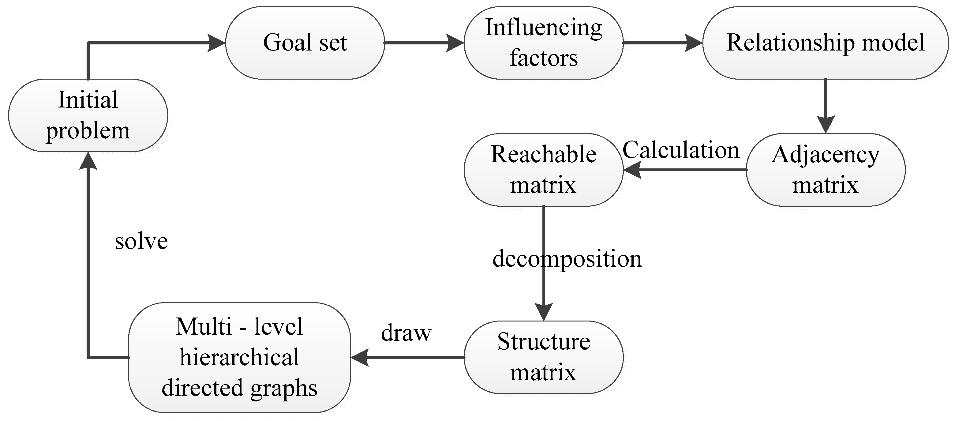
The Interpretative Structural Model is a special research method used to analyze the correlation structure of complex elements in educational technology research [10], with the role of revealing the internal structure using known relationships among the system elements. The ISM was improved in this paper (based on the relation graph of the reachability matrix) to select the operational outcome index from the top down and the operation driving index from the bottom up, before checking the selection index using the principal component analysis method. The working process of the ISM can be divided into the decision making stage and calculation process, which is shown in Figure 1.
2.3. Operational Efficiency Evaluation Model Based on Dynamic Data Envelopment Analysis (D-DEA)
Data Envelopment Analysis, which is based on the concept of relative efficiency, can be used in efficiency evaluation as a non-parametric statistical method to evaluate the efficiency of decision-making units with the same type of multiple input and output [11,12,13]. The idea is to regard an economic system as a unit (called a Decision Making Unit (DMU)), and make a “product” by putting in production factors on the grandest scale possible. The evaluation group is composed of DMUs where through the analysis of input or output ratio, evaluation variables are index weights of the DMU. Next, the efficient production frontier is determined and the validity of each DMU can be known by the distance between the DMU and the frontier. At the same time, the projection method can be used to point out the improved direction.
For model selection, this study focused on two aspects. First, compared to other models, DEA models are not only used to obtain the efficiency of each DMU, but also to solve problems where the data contain negative values due to their translation invariance. Second, Tone and Tsutsui [14] classified the constraints of linking two types: the free link and the fixed link. With respect to the free link case, the linking activities were freely determined whilst continuity between the input and output was maintained. This case demonstrated whether the current link flow was appropriate in light of the other DMUs. With respect to the fixed link case, the linking activities were kept unchanged.
This model also considered the time continuity of enterprise development, which means that the grid construction effect of the last time-period is the initial condition of the next time. The management efficiency evaluation model is dynamic, and so defined as the Dynamic Data Envelopment Analysis. At the same time, it considers the relevance of different attributes, that is, the benefit of construction investment from a property may become the investment of another property. Thus, the target function of the D-DEA was as follows:
where is the value of the input index in year; is the value of output index in year; is the slack variable of input index in year; and is the slack variable of output index in year.
The constraint conditions were as follows:
where indicates the associated value of decision-making unit from attribute to attribute during period. represents the influence value of attribute from to .
Through optimization and adjustment, the setting parameters were changed as follows:
The efficiency value of each DMU was obtained with Equation (5):
Among them, the efficiency value of each attribute of the DMU was calculated:
2.4. Operational Efficiency Evaluation Model Based on Stochastic Frontier Function
Combined with cost and production functions, SFM can be used to realize the allocation efficiency evaluation. The Douglas’s cost function with stochastic frontier characteristics can be defined as [15,16,17]:
where is the total cost of grid enterprise in the period; is the price of input factor for grid enterprise in the period; is the input factor for grid enterprise in the period and is only or ; and is the type of input element.
From Equation (7), if the cost function was used to evaluate the allocation efficiency, the known price information of the input elements is the primary condition. To avoid the price information demand of the input elements as per the inherent duality between the Cobb-Douglas production and cost function, the following optimization model as established by combining Equation (8).
The objective function of Equation (8) was to minimize the cost, and the constraint condition indicated that the input–output met the condition of the Cobb-Douglas production function. Taking the production function of the input element into consideration, the extremum problem of this condition was solved with Lagrange’s function.
By obtaining the exponential function from the production function, we can see
The coefficient was calculated by
The obtained parameter function was brought into the original formula, and the unknown parameters were eliminated, so the new cost function became
Based on the general form of the Cobb-Douglas production function, we know that the cost efficiency is the exponential term of cost function. Therefore, the cost efficiency, technical efficiency, and allocation efficiency were obtained by
3. Results and Discussion
By using the actual operation monitoring index of the State Grid Corporation as a case study, 32 relevant indicators with the highest attention were selected in operation, and the specific corresponding relationships of the indicators are shown in Table 1.
3.1. Identification and Verification of Dual Index in Power Grid Enterprises
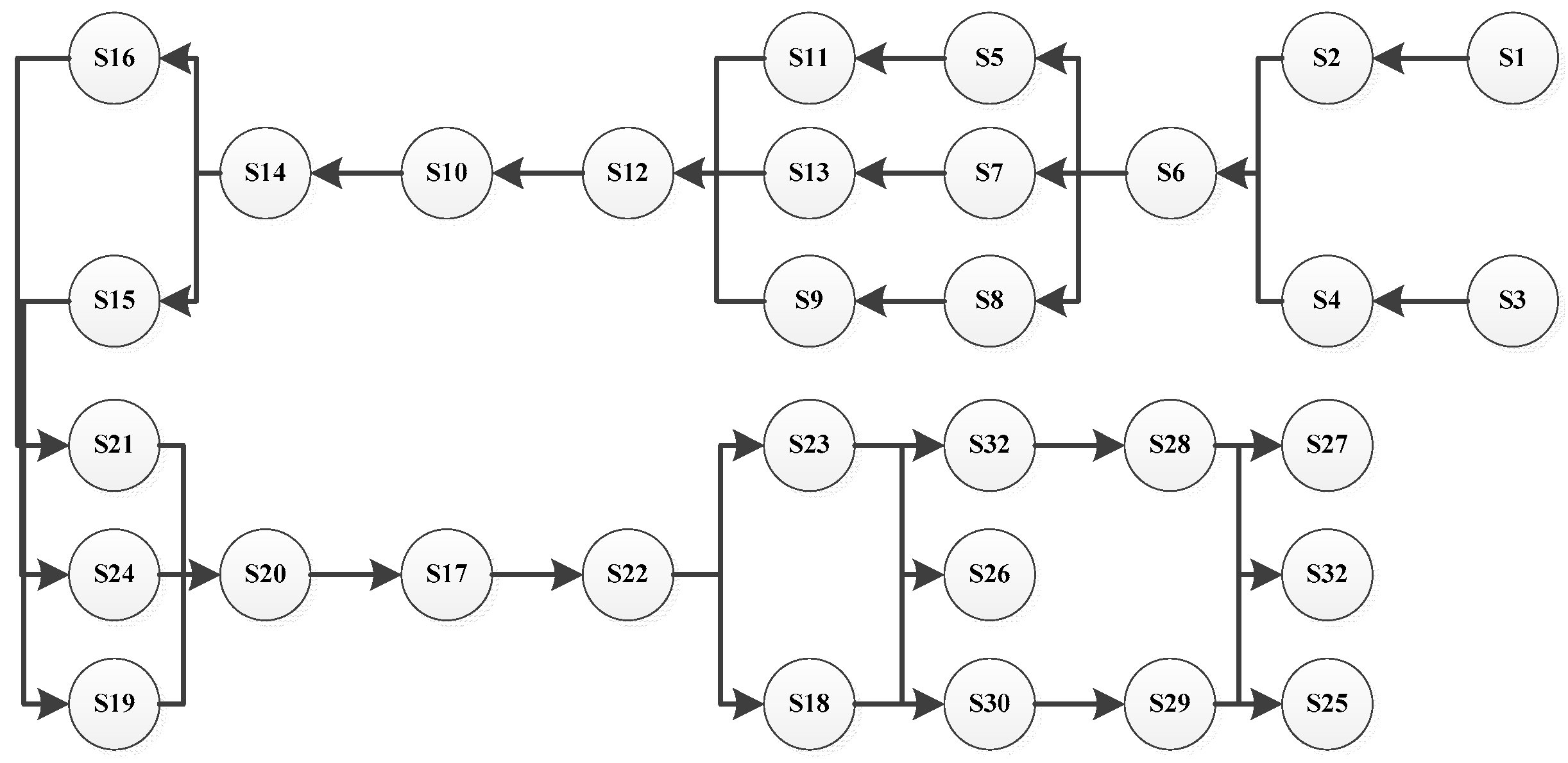
First, the index system was analyzed, and the element relation was constructed as per the relationship among indexes determined by expert grading. Next, an adjacency matrix was established based on this relationship (Figure 2), and a reachability matrix was calculated through the matrix operation (Figure 3).
Finally, the reachability matrix was decomposed under the condition of , and the relation diagram was constructed based on the result (Figure 1).
As seen in Figure 4, the 32 indexes were distributed at two ends of the level, which meant that the element closer to the top was more likely to be affected, so had great dependence; and the element closer to the bottom was more likely to impact others, so had great driving force. Two core indicators were divided under different requirements: the achievement index group and the driving index group (specific indicators are shown in Table 2).
The data was analyzed by SPSS, and to test whether 16 core indicators from the structural model could achieve a contribution rate of more than 85%. Based on the software results (Table 3), the contribution rate was more than 85%, which meant that the extracted index by the structural model could represent the operational monitoring index of a power grid.
3.2. Operational Efficiency Evaluation of Power Grid Enterprises
(1) Driving index evaluation
We comprehensively evaluated eight driving indicators, and the results using SPSS software are shown in Table 4.
Based on the processing results, we calculated the comprehensive evaluation model, as shown in the formula:
where is comprehensive score; and indicates the standard value of driving indicator i.
(2) Achievement index evaluation
We also comprehensively evaluated eight achievement indicators, and the results using SPSS software are shown in Table 5.
Based on the processing results, we calculated the comprehensive evaluation model shown in the formula:
where is the comprehensive score; and indicates the standard value of achievement indicator i.
Based on the comprehensive evaluation model of the driving and achievement indexes, the index scores were calculated in combination with nearly six years of standard data. The trend chart is shown in Figure 5.
From Figure 5, the driving index of operational performance had a rising trend. Although the achievement index as basically the same, there were some differences, especially shown by the different trends in 2011 and 2012. This difference showed that the driving index was not only the influencing factor of the achievement index, but the most important one. Thus, the index analysis could be replaced by the driving and achievement indexes, which could greatly reduce the amount of computation and improve efficiency. Combined with the general trend and efficiency evaluation of the driving and achievement indexes, it could release an early warning signal and make recommendations.
3.3. Operational Efficiency Evaluation of Power Grid Enterprises
(1) Comparison of operating efficiency over the years
We used the driving index as the input index, and the achievement index as the output index. When considering the availability of the indicators, the output index was added, including the increased supply load of unit investment, the increased consumption of unit investment, and the transmission cost of unit quantity. Next, a company’s operational efficiency was analyzed and some improvements made based on the evaluation results.
First, actual data were collected from 2008 to 2013. The mixed distance function and bidirectional priority of input–output were used in the calculation. The result showed that annual efficiency evaluations were 1 from 2008 to 2013, and the scale returns were stable. Thus, the technical efficiency and scale benefit scores of this enterprise were 1, which meant it was well controlled in input–output proportion. At the same time, it also showed that input decision and post management were reasonable and had achieved good operating efficiency.
(2) Operational efficiency comparison among enterprises
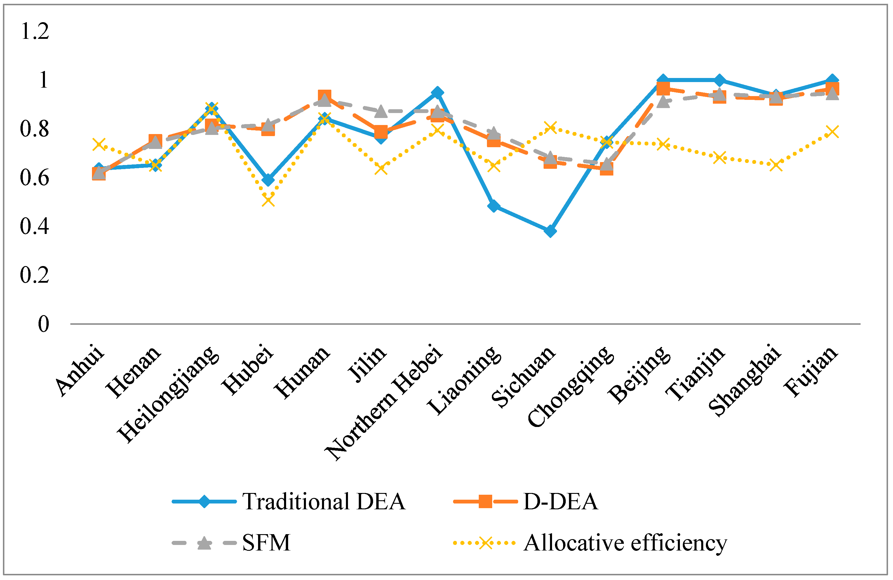
As the contrast of operational efficiency can improve the investment decision, we selected 14 provincial companies to calculate their efficiency based on data from 2013. The mixed distance function and bidirectional priority of input–output were also selected, and the operation results are shown in Table 6 and Figure 6.
Where, DMU is abbreviation of Decision Making Unit; DEA is abbreviation of Data Envelopment Analysis; D-DEA is abbreviation of Dynamic Data Envelopment Analysis; SFM is abbreviation of Stochastic Frontier Model.
From Table 6 and Figure 6, we observed that the results were similar to the improved DEA and SFM methods when calculating technical efficiency over one year; therefore, the two improved methods could provide a good solution when the efficiency of the DMU was 1.
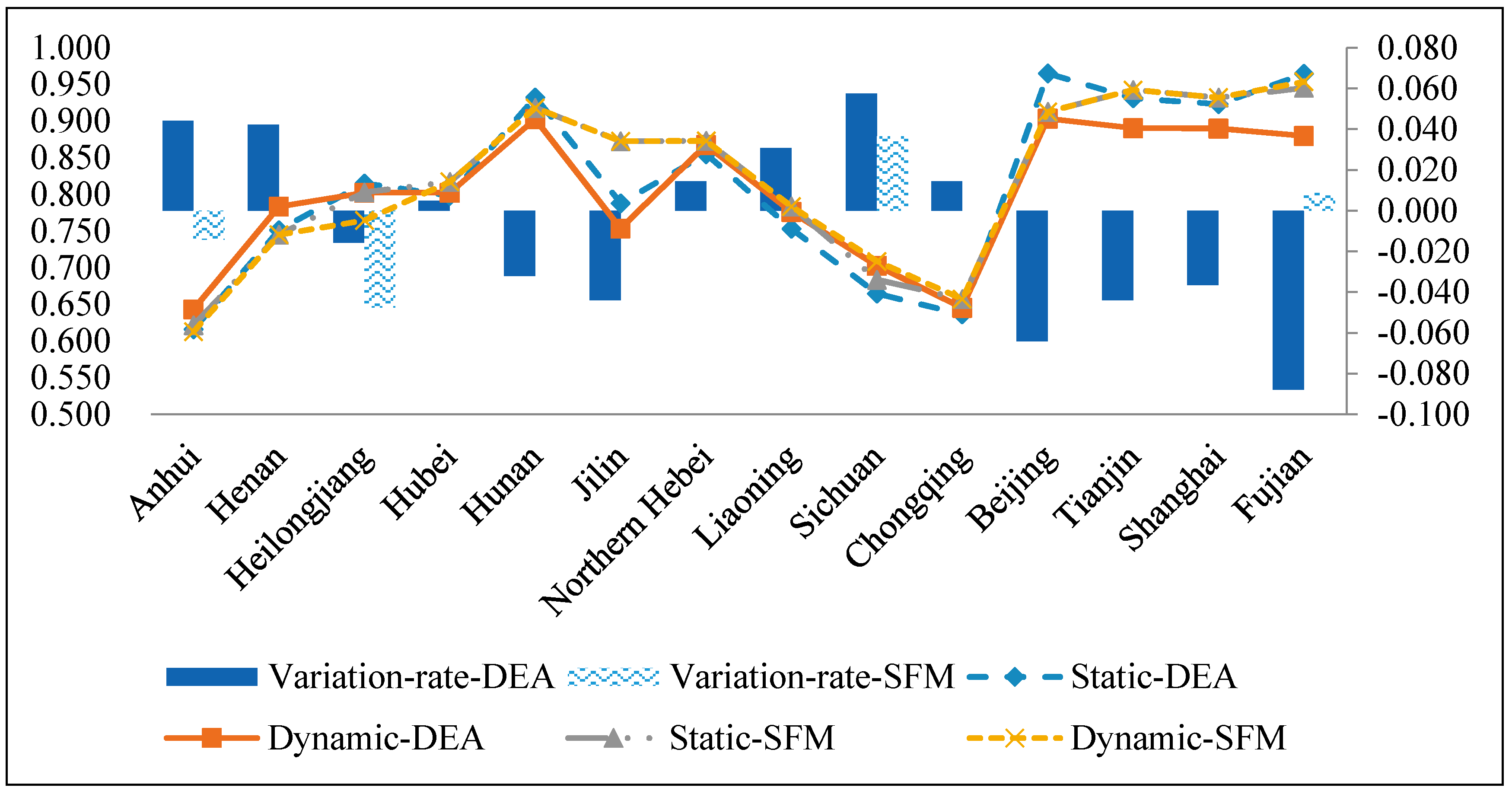
To better compare the two improved methods, we designed an efficiency linkage evaluation to account for many years, which considered the return delay of power grid investment. Through the technical efficiency calculation of each region, the results of the static efficiency and dynamic efficiency were compared, as shown in Table 7 and Figure 7.
From Table 7 and Figure 7, when considering the delay of grid investment, the dynamic and static evaluation results changed with the improved DEA method, and was relatively reasonable for the certain particularities of power grid investment, which include the large scale of fixed assets, long investment cycle, influence of grid structure, and regional economy. Therefore, it was not scientific to evaluate the static efficiency of power grid enterprises, and instead, dynamic efficiency evaluation should be adopted.
Results with a high efficiency declined and increased with low assessment results. Although there was more investment in a low assessment region in 2013, the income was not obvious, and the efficiency evaluation results were low. When considering the delay of investment benefit, the dynamic calculation obtained a higher evaluation efficiency.
Through the comparison of static and dynamic evaluation efficiency, the improved DEA model considered the impact of the previous year's investment on the operating result of the following year. Using Henan Province as an example, by comparing the static and dynamic efficiency evaluation of the two methods, the dynamic efficiency evaluation result improved with the modified DEA method that considered power grid structure and regional economic factors; the results of the dynamic efficiency evaluation did not change with the SFM model, which indicated that these factors were not taken into account. Therefore, the improved DEA model was more consistent with the factual data.
4. Conclusions
The operational monitoring service of a power grid enterprise is pioneering work in the control practice of large enterprise groups. This paper evaluated the operational efficiency of power grid enterprises, and obtained the following conclusions:
- The index concerned with power grid enterprises may reach hundreds of items. The monitoring index system and identification method used in this study played a guiding role in simplifying the index.
- The key indicator identification method in this paper is feasible and applicable to power grid enterprises, and plays a supporting role in improving operations monitoring and the decision making technology of power grid enterprises.
- This paper compared the effectiveness of SFM, traditional DEA, and D-DEA for operational efficiency evaluations. Results showed that D-DEA had a stronger rationality when compared with the static efficiency evaluation where the average change ratio was 4% of the dynamic efficiency evaluation results.
The method proposed in this paper not only is applicable to the efficiency evaluation of regional power grids, but can also be applied to efficiency evaluations of district heating and cooling networks. And, there is still plenty of improved space for model design methods in further study, and is the subject of future research.
Acknowledgments
The paper is supported by the Fundamental Research Funds for the Central Universities 2016XS82, the National Science Foundation of China (Grant No.: 71273090, 71573084), the Beijing Municipal Social Science Foundation (16JDYJB044), and the Science and Technology Project of State Grid Corporation (Research on Application Technology and Model of Big Data in Key Fields of the Company).
Author Contributions
Yixin Sun, Qingyou Yan and Zhongfu Tan conceived and designed the experiments; Xiaobao Yu performed the experiments; Qingyou Yan and Zhongfu Tan analyzed the data; Yixin Sun contributed analysis tools and collected data; Xiaobao Yu and Xiaofei Xu wrote the paper and modificated the paper.
Conflicts of Interest
The authors declare no conflict of interest.
Nomenclature
| DMU | Decision Making Unit |
| D-DEA | Dynamic Data Envelopment Analysis |
| ISM | Interpretive Structural Model |
| SFM | Stochastic Frontier Model |
| i | input index |
| r | output index |
| j | Decision Making Unit |
| t | time |
| k | division |
| s | input factors category |
| x | the value of input index |
| y | the value of output index |
| S | slack variable |
| z | the associated value |
| efficiency value | |
| C | cost |
| p | price |
| l | labor force |
| v | random error |
| u | non-technical efficiency |
| elasticity coefficient of input index | |
| elasticity coefficient of labor force | |
| A | constant |
References
- Yu, X.; Tan, Z. Differentiated Evaluation of Smart Grid in the Improved Hall Three-Dimensional Perspective. Mod. Electr. Power 2015, 4, 42–48. [Google Scholar]
- Yan, Z.; Li, L.; Han, D.; Chen, H.; Yu, N. Evaluation Model for Low-carbon Electricity Production on Efficiency Based on Improved Super Efficiency Data Envelopment Analysis Method. Dianli Xitong Zidonghua Autom. Electr. Power Syst. 2014, 17, 170–176. [Google Scholar]
- Han, D.; Yan, Z.; Li, L. An Evaluation Method for Efficiency of Smart Grids Based on Stochastic Frontier Model. Power Syst. Technol. 2015, 7, 1963–1969. [Google Scholar]
- Jha, D.K.; Shrestha, R. Measuring efficiency of hydropower plants in Nepal using data envelopment analysis. IEEE Trans. Power Syst. 2006, 21, 1502–1511. [Google Scholar] [CrossRef]
- Price Cap Regulation in the Electricity Sector; Netherland Electricity Regulatory Service: Hague, The Netherlands, 1999.
- Liu, Y.; Gu, H. Research on risk control system in regional power grid. In Proceedings of the 2012 China International Conference on Electricity Distribution (CICED), Shanghai, China, 10–14 September 2012. [Google Scholar]
- Sun, Q.; Ye, J.H.; Li, N.; Chen, H.; Jin, X.; Wang, J.; Yao, J.G. Study on the effect of high-speed railway traction power supply system on real-time power grid operation. J. Hunan Univ. Nat. Sci. 2012, 10, 50–55. [Google Scholar]
- Kaplan, R.S.; Norton, D.P. The Balanced Scorecard: Translating Strategy into Action. J. Prod. Innov. Manag. 1997, 14, 235–237. [Google Scholar]
- Li, J.-X.; Hu, F.; Liu, Z.-H. A New Loan Project Performance Evaluation Model of the Commercial Bank. J. Hunan Univ. Nat. Sci. 2010, 2, 83–87. [Google Scholar]
- Han, J.-S.; Tan, Z.-F.; Liu, Y. Research on Interpratative Structure Modeling for Risks of Electricity Retail Market. Power Syst. Technol. 2005, 8, 14–19. [Google Scholar]
- Yang, G.; Liu, W.; Zheng, H. Review of Data Envelopment Analysis. J. Syst. Eng. 2013, 6, 840–860. [Google Scholar]
- Guo, Z.; Wu, J.; Kong, F. Multi-objective Optimization Scheduling for Hydrothermal Power Systems Based on Electromagnetism-like Mechanism and Data Envelopment Analysis. Proc. Chin. Soc. Electr. Eng. 2013, 4, 53–61. [Google Scholar]
- Liu, S.; Du, S.-X. Fuzzy Comprehensive Evaluation Based on Data Envelopment Analysis. Fuzzy Syst. Math. 2010, 2, 93–98. [Google Scholar]
- Tone, K.; Tsutsui, M. Network DEA: A slacks-based measure approach. Eur. J. Oper. Res. 2009, 197, 243–252. [Google Scholar] [CrossRef]
- Li, C.-B.; Li, P.; Lu, G.-S. Comprehensive Evaluation of Smart Grid Operation Risk Based on Fuzzy Number Similarity. East China Electr. Power 2012, 9, 1486–1489. [Google Scholar]
- Cai, Y. Research and Application of Data Mining Technology in Grid Operational Monitoring Platform; Shanghai Jiaotong University: Shanghai, China, 2013. [Google Scholar]
- Kılıç, D.; Sağlam, N. Students’ understanding of genetics concepts: The effect of reasoning ability and learning approaches. J. Boil. Educ. 2014, 48, 63–70. [Google Scholar] [CrossRef]
Figure 1.
Basic workflow of the Interpretive Structural Model (ISM).

Figure 2.
Adjacency matrix.
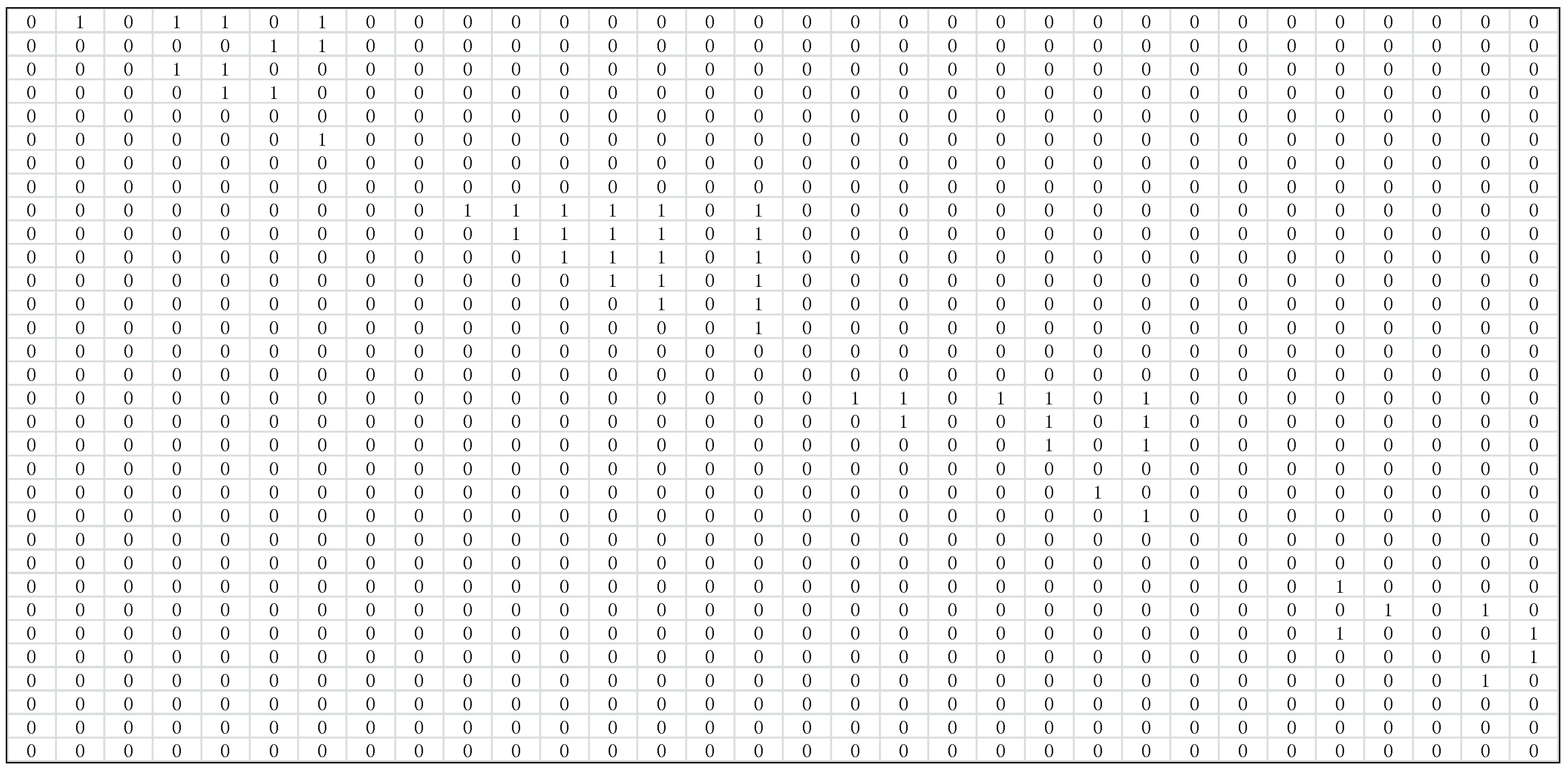
Figure 3.
Reachability matrix.
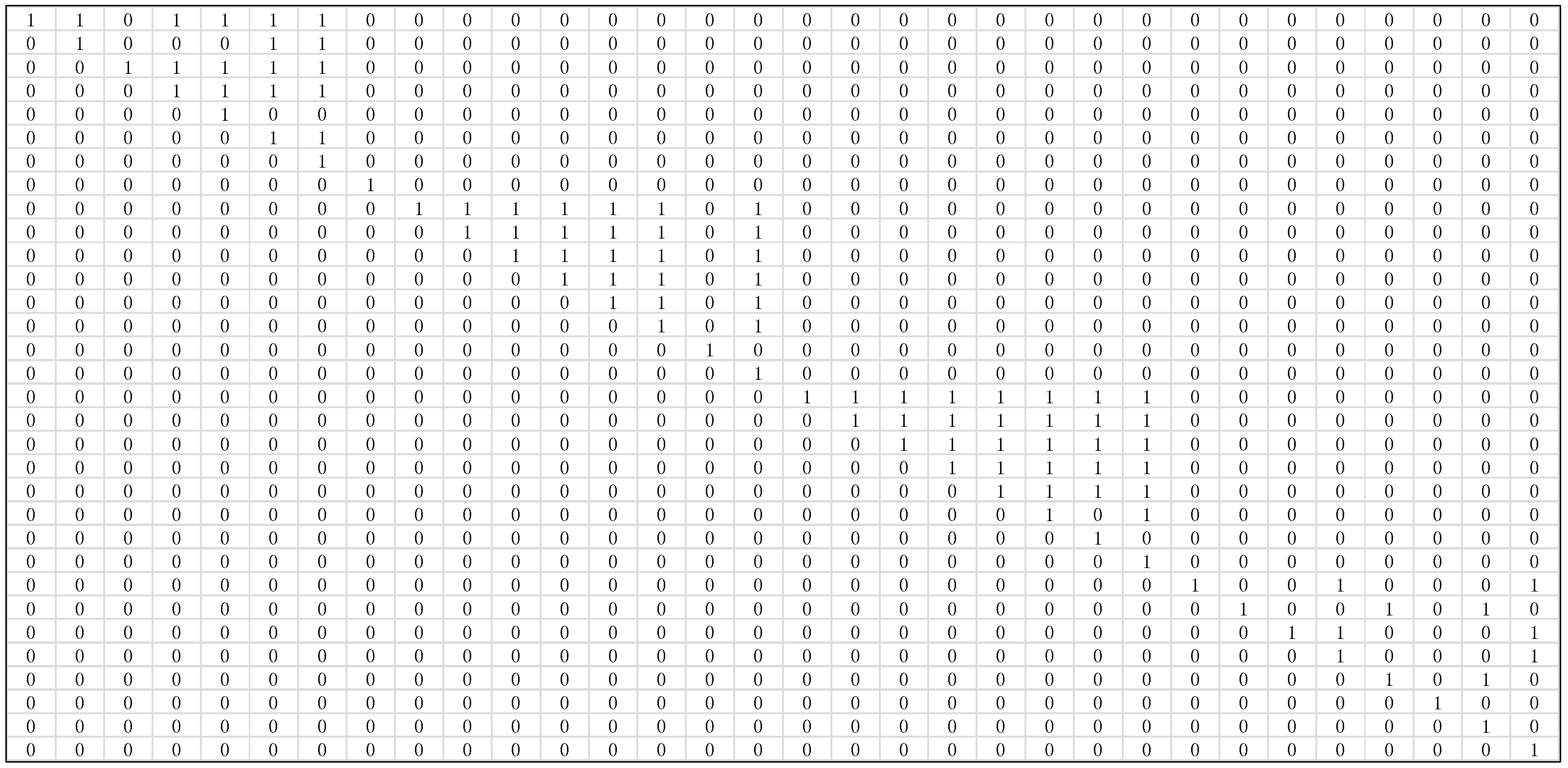
Figure 4.
Relationship diagram of the operational monitoring index.

Figure 5.
Comprehensive trend of operational performance driving index and achievement index.
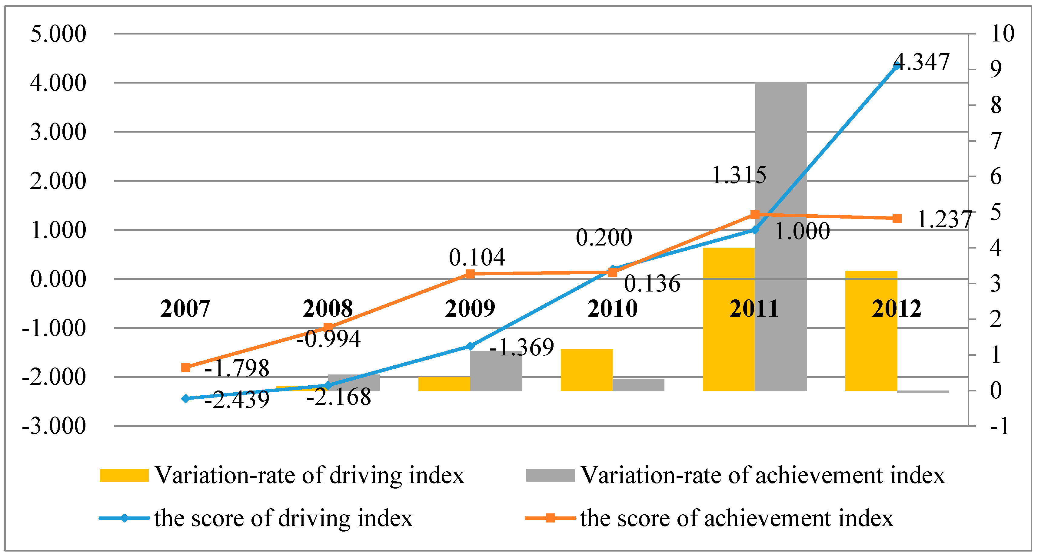
Figure 6.
A comparison of the efficiency evaluation results.

Figure 7.
Evaluation comparison of static efficiency and dynamic efficiency.

Table 1.
Correspondence relation for index definition.
| Index | Definition | Index | Definition |
|---|---|---|---|
| Power grid investment | S1 | Maintenance cost of power grid | S17 |
| Infrastructure investment | S2 | Industrial added value | S18 |
| Line length of per capita | S3 | Transmission and distribution cost | S19 |
| Total staff | S4 | Load rate | S20 |
| Technological transformation investment | S5 | Inventory turnover | S21 |
| Average price difference of power purchasing and selling | S6 | Outage rate of power grid system | S22 |
| Marketing investment | S7 | Inventory material idle rate | S23 |
| Grid-connected installed capacity of new energy | S8 | Talent equivalent density | S24 |
| Electricity recovery rate | S9 | Electricity sales | S25 |
| Market share | S10 | Per capita profit | S26 |
| Gross income | S11 | Economic value added | S27 |
| Reliability rate of power supply | S12 | Comprehensive line loss rate | S28 |
| Customer satisfaction rate | S13 | Voltage qualification rate | S29 |
| Power supply population | S14 | Return on equity | S30 |
| Emission reduction CO2 by generation right transaction | S15 | Total owners’ equity | S31 |
| Execution equilibrium rate of Electricity Purchase Contracts | S16 | Asset-liability ratio | S32 |
Table 2.
Achievement index group and driving index group.
| Driving Index Group | Achievement Index Group | ||
|---|---|---|---|
| Number | Index | Number | Index |
| 1 | Power grid investment | 1 | Comprehensive line loss rate |
| 2 | Infrastructure investment | 2 | Voltage qualification rate |
| 3 | Line length of per capita | 3 | Asset-liability ratio |
| 4 | Total staff | 4 | Per capita profit |
| 5 | Technological transformation investment | 5 | Economic value added |
| 6 | Average price difference of power purchasing and selling | 6 | Electricity sales |
| 7 | Marketing investment | 7 | Total owners’ equity |
| 8 | Grid-connected installed capacity of new energy | 8 | Return on equity |
Table 3.
Contribution rate of core index and total amount.
| Core Index | Power Grid Investment | Infrastructure Investment | Line Length of Per Capita | Total Staff | Technological Transformation Investment | Average Price Difference of Power Purchasing and Selling | Marketing Investment | Grid-Connected Installed Capacity of New Energy |
| Contribution rate | 0.0918 | 0.0789 | 0.0625 | 0.0611 | 0.0546 | 0.0421 | 0.0376 | 0.103 |
| Cumulative contribution rate | 0.0918 | 0.1707 | 0.2332 | 0.2943 | 0.3489 | 0.391 | 0.4286 | 0.5316 |
| Comprehensive line loss rate | Voltage qualification rate | Asset-liability ratio | Per capita profit | Economic value added | Electricity sales | Total owners’ equity | Return on equity | |
| 0.0727 | 0.0672 | 0.0535 | 0.0416 | 0.0382 | 0.0339 | 0.0235 | 0.011 | |
| 0.6043 | 0.6715 | 0.725 | 0.7666 | 0.8048 | 0.8387 | 0.8622 | 0.8732 | |
Table 4.
Processing results of the driving index.
| Component | Initial Eigenvalues | Extraction Sums of Squared Loadings | ||||
|---|---|---|---|---|---|---|
| Total | % of Variance | Cumulative % | Total | % of Variance | Cumulative % | |
| 1 | 6.799 | 84.986 | 84.986 | 6.799 | 84.986 | 84.986 |
| 2 | 0.914 | 11.419 | 96.405 | |||
| 3 | 0.162 | 2.020 | 98.425 | |||
| 4 | 0.116 | 1.451 | 99.875 | |||
| 5 | 0.010 | 0.125 | 100.000 | |||
| 6 | 3.01E-16 | 3.766E-15 | 100.000 | |||
| 7 | 1.72E-16 | 2.155E-15 | 100.000 | |||
| 8 | −2.71E-17 | −3.3394E-16 | 100.000 | |||
Extraction Method: Principal Component Analysis.
Table 5.
Processing results of the achievement index.
| Component | Initial Eigenvalues | Extraction Sums of Squared Loadings | ||||
|---|---|---|---|---|---|---|
| Total | % of Variance | Cumulative % | Total | % of Variance | Cumulative % | |
| 1 | 4.091 | 51.139 | 51.139 | 4.091 | 51.139 | 51.139 |
| 2 | 2.225 | 27.813 | 78.952 | 2.225 | 27.813 | 78.952 |
| 3 | 1.006 | 12.579 | 91.530 | 1.006 | 12.579 | 91.530 |
| 4 | 0.549 | 6.868 | 98.399 | |||
| 5 | 0.128 | 1.601 | 100.000 | |||
| 6 | 1.24E-16 | 1.560E-15 | 100.000 | |||
| 7 | −7.45E-17 | −9.323E-16 | 100.000 | |||
| 8 | −1.67E-16 | −2.094-15 | 100.000 | |||
Extraction Method: Principal Component Analysis.
Table 6.
Regional efficiency assessment.
| Number | DMU | Technical Efficiency | Allocative Efficiency | Return of Scale | ||
|---|---|---|---|---|---|---|
| Traditional DEA | D-DEA | SFM | ||||
| 1 | Anhui | 0.636429 | 0.615978 | 0.621734 | 0.736429 | Growing |
| 2 | Henan | 0.651479 | 0.751509 | 0.745261 | 0.651479 | Growing |
| 3 | Heilongjiang | 0.88382 | 0.815186 | 0.802847 | 0.88382 | Growing |
| 4 | Hubei | 0.590821 | 0.798534 | 0.817264 | 0.50821 | Growing |
| 5 | Hunan | 0.842656 | 0.932699 | 0.918274 | 0.842656 | Growing |
| 6 | Jilin | 0.763904 | 0.788218 | 0.872734 | 0.63904 | Growing |
| 7 | Northern Hebei | 0.94921 | 0.855103 | 0.873212 | 0.794921 | Growing |
| 8 | Liaoning | 0.484767 | 0.75323 | 0.783621 | 0.64923 | Growing |
| 9 | Sichuan | 0.380624 | 0.664676 | 0.683762 | 0.80624 | Growing |
| 10 | Chongqing | 0.745368 | 0.636271 | 0.657261 | 0.745368 | Growing |
| 11 | Beijing | 1 | 0.965293 | 0.912837 | 0.738273 | Stable |
| 12 | Tianjin | 1 | 0.931343 | 0.942812 | 0.682763 | Stable |
| 13 | Shanghai | 0.937281 | 0.923472 | 0.932321 | 0.652734 | Growing |
| 14 | Fujian | 1 | 0.964716 | 0.945627 | 0.789321 | Stable |
Table 7.
Comparison of static and dynamic results for efficiency evaluation.
| Number | DMU | D-DEA | Variation Rate | SFM | Variation Rate | ||
|---|---|---|---|---|---|---|---|
| Static | Dynamic | Static | Dynamic | ||||
| 1 | Anhui | 0.616 | 0.643 | 0.044 | 0.622 | 0.613 | –0.014 |
| 2 | Henan | 0.752 | 0.783 | 0.042 | 0.745 | 0.745 | 0.000 |
| 3 | Heilongjiang | 0.815 | 0.802 | −0.016 | 0.803 | 0.765 | –0.048 |
| 4 | Hubei | 0.799 | 0.802 | 0.005 | 0.817 | 0.817 | 0.000 |
| 5 | Hunan | 0.933 | 0.903 | −0.032 | 0.918 | 0.918 | 0.000 |
| 6 | Jilin | 0.788 | 0.754 | −0.044 | 0.873 | 0.873 | 0.000 |
| 7 | Northern Hebei | 0.855 | 0.867 | 0.014 | 0.873 | 0.873 | 0.000 |
| 8 | Liaoning | 0.753 | 0.776 | 0.031 | 0.784 | 0.784 | 0.000 |
| 9 | Sichuan | 0.665 | 0.703 | 0.057 | 0.684 | 0.709 | 0.037 |
| 10 | Chongqing | 0.636 | 0.645 | 0.014 | 0.657 | 0.657 | 0.000 |
| 11 | Beijing | 0.965 | 0.903 | −0.064 | 0.913 | 0.913 | 0.000 |
| 12 | Tianjin | 0.931 | 0.890 | −0.044 | 0.943 | 0.943 | 0.000 |
| 13 | Shanghai | 0.923 | 0.890 | −0.036 | 0.932 | 0.932 | 0.000 |
| 14 | Fujian | 0.965 | 0.880 | −0.088 | 0.946 | 0.954 | 0.009 |
© 2017 by the authors. Licensee MDPI, Basel, Switzerland. This article is an open access article distributed under the terms and conditions of the Creative Commons Attribution (CC BY) license (http://creativecommons.org/licenses/by/4.0/).
Share and Cite
MDPI and ACS Style
Sun, Y.; Yu, X.; Tan, Z.; Xu, X.; Yan, Q. Efficiency Evaluation of Operation Analysis Systems Based on Dynamic Data Envelope Analysis Models from a Big Data Perspective. Appl. Sci. 2017, 7, 624. https://doi.org/10.3390/app7060624
AMA Style
Sun Y, Yu X, Tan Z, Xu X, Yan Q. Efficiency Evaluation of Operation Analysis Systems Based on Dynamic Data Envelope Analysis Models from a Big Data Perspective. Applied Sciences. 2017; 7(6):624. https://doi.org/10.3390/app7060624
Chicago/Turabian StyleSun, Yixin, Xiaobao Yu, Zhongfu Tan, Xiaofei Xu, and Qingyou Yan. 2017. "Efficiency Evaluation of Operation Analysis Systems Based on Dynamic Data Envelope Analysis Models from a Big Data Perspective" Applied Sciences 7, no. 6: 624. https://doi.org/10.3390/app7060624
Note that from the first issue of 2016, this journal uses article numbers instead of page numbers. See further details here.