
Soliton Content of Fiber-Optic Light Pulses

Institut für Physik, Universität Rostock, A.-Einstein-Str. 23, 18059 Rostock, Germany
*
Author to whom correspondence should be addressed.
†
These authors contributed equally to this work.
Appl. Sci. 2017, 7(6), 635; https://doi.org/10.3390/app7060635
Submission received: 11 May 2017
/
Revised: 8 June 2017
/
Accepted: 11 June 2017
/
Published: 19 June 2017
(This article belongs to the Special Issue Guided-Wave Optics)
Abstract
:This is a review of fiber-optic soliton propagation and of methods to determine the soliton content in a pulse, group of pulses or a similar structure. Of central importance is the nonlinear Schrödinger equation, an integrable equation that possesses soliton solutions, among others. Several extensions and generalizations of this equation are customary to better approximate real-world systems, but this comes at the expense of losing integrability. Depending on the experimental situation under discussion, a variety of pulse shapes or pulse groups can arise. In each case, the structure will contain one or several solitons plus small amplitude radiation. Direct scattering transform, also known as nonlinear Fourier transform, serves to quantify the soliton content in a given pulse structure, but it relies on integrability. Soliton radiation beat analysis does not suffer from this restriction, but has other limitations. The relative advantages and disadvantages of the methods are compared.
1. Introduction
Light pulses in optical fibers carry the bulk of all telecommunication today. In comparison to electrical pulses in cables, fiber-optic transmission is vastly superior, mostly due to two fundamental advantages: light in fibers suffers extremely low power loss, and fibers provide an extremely wide bandwidth. For the loss, a rough number is . This implies that even after 100 km, still, 1% of the launch power is left, which is unrivaled. The available bandwidth can be estimated as (maybe if one accepts slightly higher loss), which is several orders of magnitude better than anything that can be achieved with electronics.
Further comparison of optical and electrical transmission brings us to an imperfection shared by both: in either type of conduit, group velocity depends on frequency; as any signal requires a certain bandwidth, transmitted signals suffer from distortion due to group velocity dispersion. This is a linear distortion, which means that it can be perfectly compensated by adding an element of opposite dispersion.
In one respect, however, optical fibers are very different from electrical cables. The response of glass to light is nonlinear, whereas that of copper to current is not (within reasonable limits). Therefore, the physics of data transmission with light pulses through optical fibers is fundamentally different in that it involves a nonlinear response of the material to the signal [1,2]. Nonlinear distortions are not as easily compensated as linear ones. This has led to a widely-held conception that optical power in fibers must always be kept low enough so that nonlinear distortions are avoided.
To this argument, one can give two responses: One, nonlinearity can actually be put to good use, even be used to an advantage, when the concept of solitons is adopted. It has already been demonstrated even in a commercial setting. Two, the ever-growing demand for data-carrying capacity brings us close to a capacity crunch, unless means are found in just a few years to improve technology. It may become necessary to look at solitonic formats again.
2. The Nonlinear Schrödinger Equation and Some of Its Solutions
The glass of optical fiber is a dispersive material. With the index being a function of wavelength or optical frequency, i.e., , the group velocity is also frequency dependent. The glass is also a nonlinear material. This chiefly means that the refractive index follows the instantaneous intensity, i.e., . Across the duration of a short pulse of light, the index experiences a slight modulation, which gives rise to intensity-dependent phase shifts known as self-phase modulation [3].
A propagation equation for light pulses in fibers must contain these two influences, at least in leading order. The equation that fits this description is known as the nonlinear Schrödinger equation (NLSE). It plays an absolutely central role in all of the nonlinear fiber optics. It describes the evolution of the pulse amplitude envelope (the fast oscillation at some central optical frequency is removed) in a frame of reference comoving with the traveling light, i.e., with the group velocity at . Written in physical quantities, it is given by:
Here, is the complex amplitude with z the position along the fiber and t the retarded time. is the coefficient of group velocity dispersion, and is the coefficient of nonlinearity. Depending on the situation, it may become necessary to add corrective terms for loss, higher-order dispersion or other nonlinear effects, as we shall see in Section 3.1. The equation received its name due to its formal similarity to the Schrödinger equation of quantum mechanics fame: The quantum mechanical version typically describes how a wave function spreads out in space as time goes by; here, the equation describes how a short pulse gets broadened temporally as it propagates down the fiber. Therefore, time and space coordinates switch roles. The potential, in the nonlinear case, comes from the self-phase modulation, which is captured in the nonlinear term.
The effort to find solutions to this equation benefited from the fact that the NLSE is integrable. Integrable equations have very special mathematical properties like an infinite number of preserved quantities. A first solution was found by Vladimir E. Zakharov and Aleksei B. Shabat in 1972 [4] using the inverse scattering technique, developed by Gardner et al. in 1967 [5] (see Section 4.1). It exists for a particular combination of algebraic signs of the two parameters; with always positive, one would have the correct signs for , i.e., for what is known as anomalous dispersion. Two years later, Junkichi Satsuma and Nubuo Yajima [6] treated the pertaining initial-value problem. Between them, these two papers already form a solid base of the understanding of solitons. In the time between those two, Akira Hasegawa and Frederick Tappert suggested that the NLSE was applicable to pulse propagation in optical fibers, so that fiber-optic solitons would exist [7]. At that time, optical fibers were a novelty and not yet technologically matured. Attempts to transmit light pulses for data transmission suffered from dispersive distortions. It was therefore a bold proposal that the use of solitons as signaling pulses might overcome dispersive broadening, in other words that nonlinearity could be exploited to cancel distortions arising from a linear mechanism.
Of course, the proposal required as a very first step that the existence of fiber-optic solitons be corroborated experimentally. In the anomalously dispersive regime, i.e., at wavelengths longer than ca. , they were still too lossy for any meaningful test. By 1980, this situation had improved, and Linn F. Mollenauer, Roger H. Stolen and James P. Gordon could experimentally verify the existence of solitons [8].
2.1. Soliton Solutions
2.1.1. The Fundamental Soliton
In the anomalous dispersion regime, the NLSE Equation (1) supports a stable solution known as the fundamental soliton:
Here, is the peak power; is the pulse duration; is the deviation of the soliton’s center optical frequency from that of the frame of reference, . , and are the initial values of center time, start position and phase offset, respectively. As long as a single soliton is considered, frequency offset and initial values may be set to zero without loss of generality so that a considerably simplified version:
remains. In either case, amplitude and duration are coupled and must fulfil:
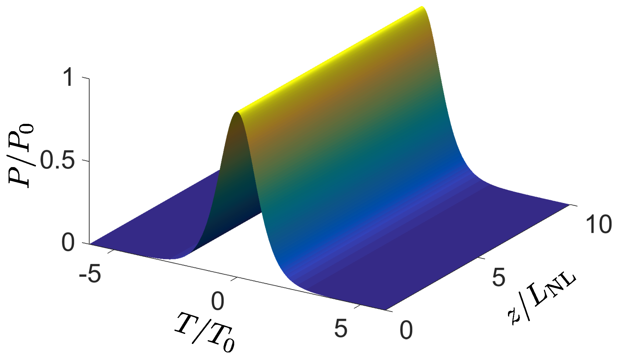
The propagation of a fundamental soliton with is shown in Figure 1. As the temporal evolution (sech term) does not contain z, the temporal shape does not change during propagation. Without nonlinearity, the shape would change appreciably after one dispersion length . The other relevant length scale is the nonlinearity length after which self-phase modulation becomes appreciable. As Equation (4) shows, for the soliton . This equality expresses the balance between both.
Among the conserved quantities of the integrable equation are the soliton energy:
and the soliton center frequency . As will be described below (Section 4.1), these two values are found from inverse scattering in the form of imaginary and real parts of a complex eigenvalue. We point out that in a dispersive medium, a nonzero frequency translates to a relative motion, so that the frequency is usually referred to as the velocity. The number of solitons is also preserved, even in cases when there is more than one.
2.1.2. Radiation and Higher-Order Solitons
To create a soliton, one can launch a sech-shaped pulse as in Equation (3) for into a fiber with parameters conforming to Equation (4). If, however, the parameters are only approximately right, we can do as follows: In the spirit of [6] and as also detailed in [9] (but they call A what we call N as in [1,2,10]), we write the initial condition as:
where the pulse is scaled by a factor , called the soliton order. The energy is then:
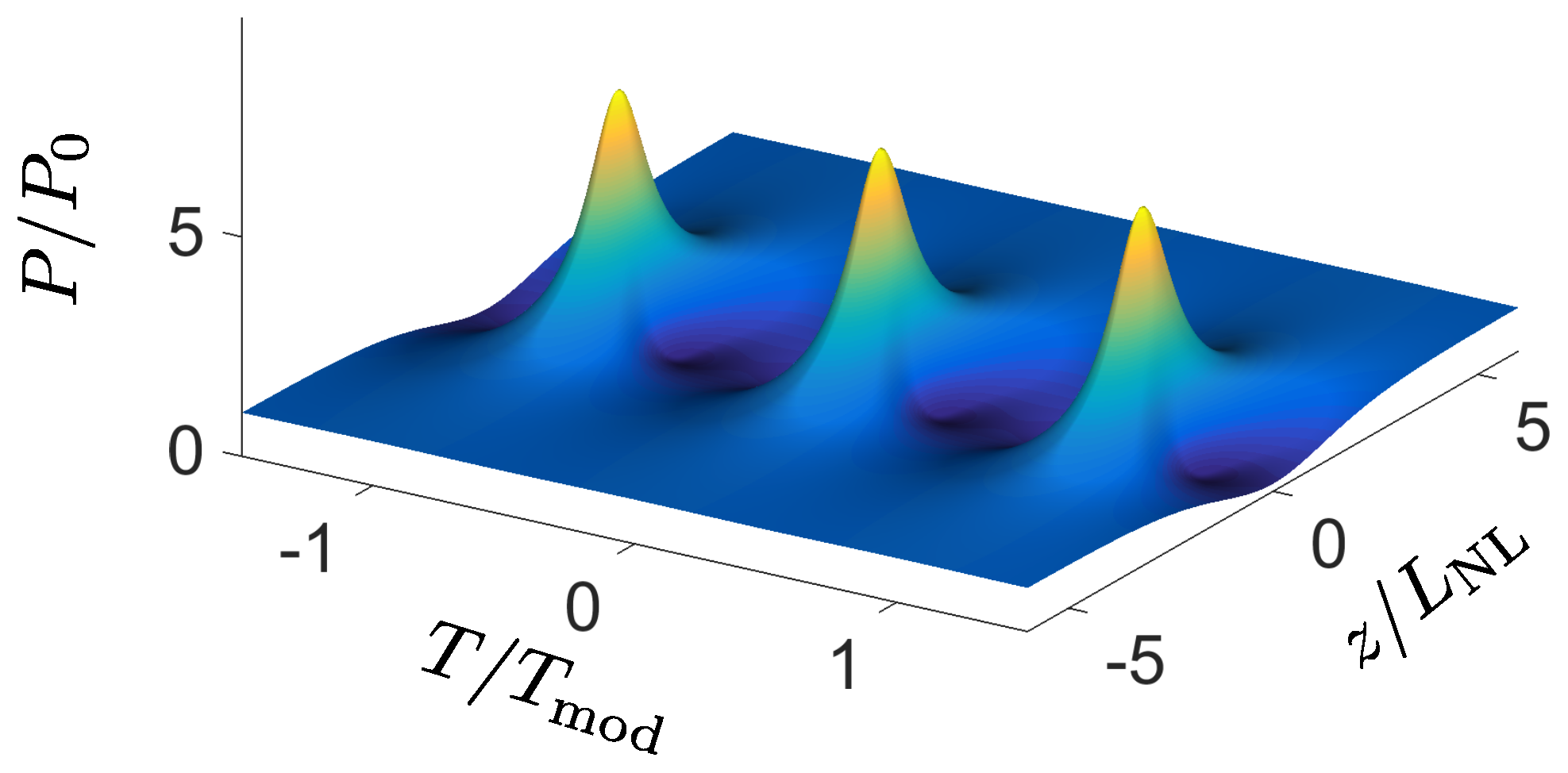
Of course, at , there is the fundamental soliton, but at non-integer N, there is also a part of the pulse energy that is not part of the soliton energy. This balance is a linear wave; in the soliton context, it is called radiation. Linear waves are subject to dispersive broadening, so that after a sufficiently long propagation, radiation will be dispersed away from the soliton, and the soliton itself emerges. Until that happens, the different phase evolution of soliton and radiation creates a beat note, visible as a slowly-decaying beat pattern. This is shown for in Figure 2 (left), where lengths are scaled to . Evaluation of the beat pattern can yield soliton parameters, see Section 4.2.
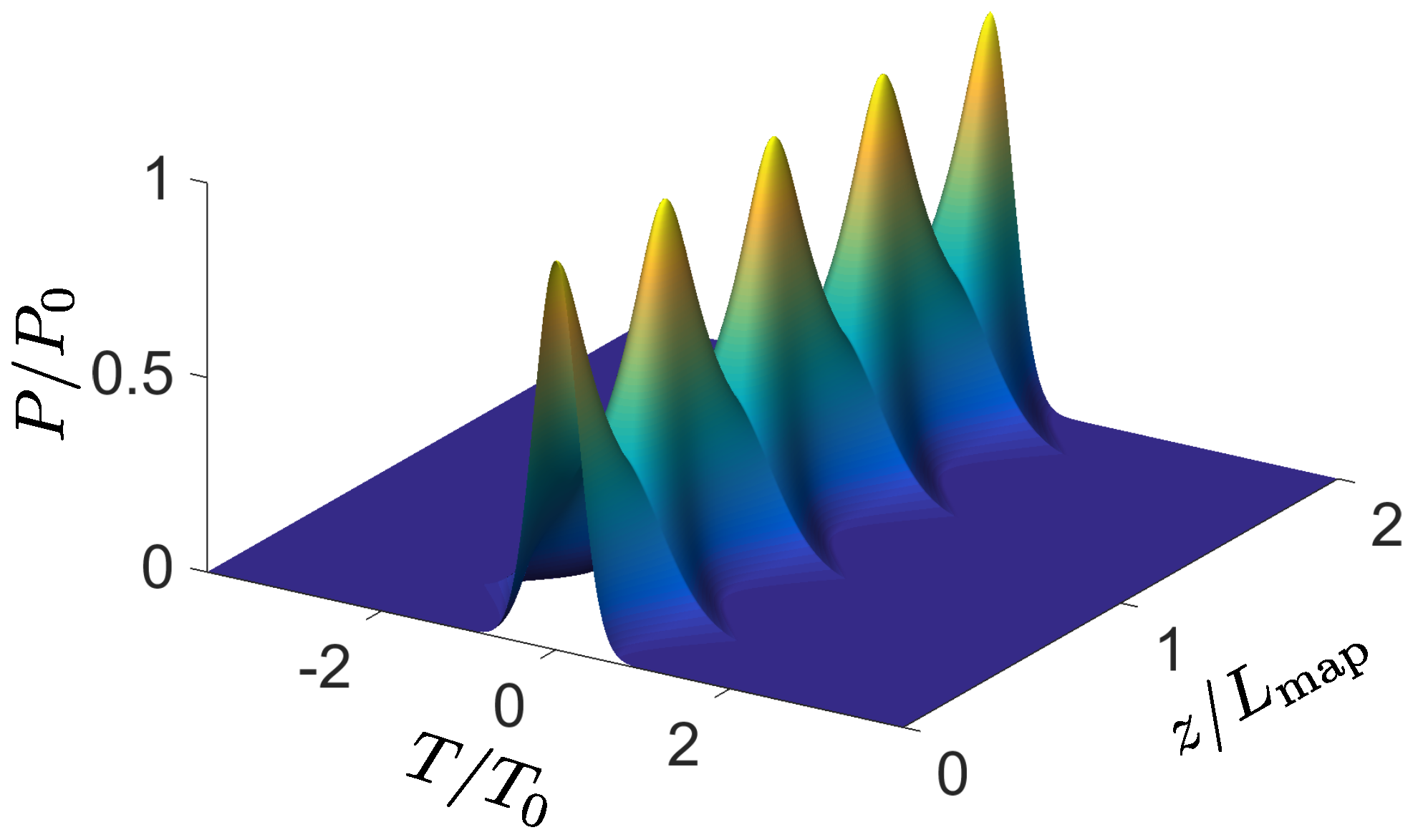
There is a threshold value of N to generate a soliton. As long as , all energy goes into radiation. At , the radiative part dips to zero. At , it reaches the same energy as at again, and that suffices to generate a second soliton. At , there is a combination of two solitons without any radiative part. This structure, for which an explicit expression was already given in [6], is called an soliton (Figure 2 right). More generally speaking, for any , , one has a so-called higher-order soliton of order N in the pure form, i.e., without radiation. An explicit expression for the case solitons was found in [11]. The power profile of all higher-order solitons oscillates with period . For all non-integer values of N, there is a radiative contribution.
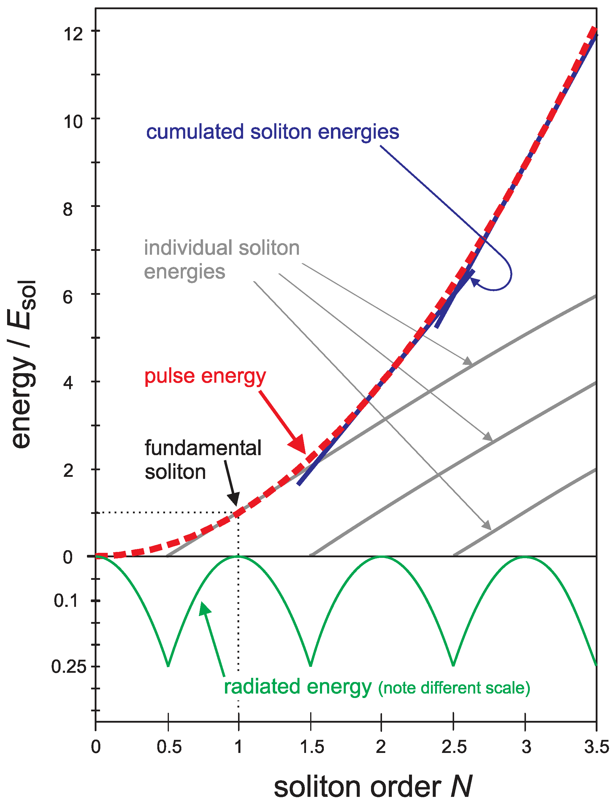
Figure 3 gives an overview of this situation. In its upper part, the pulse energy according to Equation (7), shown in units of , is represented by the dashed parabola. Beginning at , the first soliton appears. Its energy then rises linearly and passes through unity at . Similarly, at other half-integer values of N, more solitons begin, each of them contributing energy to a cumulative value shown in blue. The latter is tangent to the parabola at integer N values; here, the individual soliton energies are also integer in units. They take the first N values of the sequence , which add up to . For all non-integer N, there is a gap between the cumulative solitonic and the total energy, which represents the radiative part of the energy. Radiation energy is shown in the figure’s lower part on an inverted, magnified scale (green curve). Whenever, at some half-integer N, it reaches , the next soliton is created. Always the integer number closest to N determines the number of solitons involved, while the fractional part determines the amount of radiation created along with them.
2.1.3. Soliton Interaction
When two or more pulses are launched in rapid succession, each of them is affected by the presence of the others due to the index nonlinearity. In an integrable system, they cannot merge (the number is preserved), but they can be set in relative motion as if there were interaction forces. Gordon investigated the soliton-soliton interaction [12] and found that an effective force would decay exponentially with growing separation between pulses and vary sinusoidally with their relative phase. This means that there can be both attraction (in phase) or repulsion (opposite phase). This prediction was tested experimentally in [13] and was found to be fully correct, with the only caveat that in the attractive case, the first close encounter (collision) leads to processes of higher order not captured in the NLSE.
Note that this view of interaction forces between particles is metaphorical and justifiable only if both are well separated. In a nonlinear system, the superposition principle does not hold; therefore, two sech-shaped pulses in close proximity to each other are not really two identical, but overlapping solitons, but form a somewhat more involved two-soliton compound [14]. For that, energy and velocity are preserved quantities.
2.2. Breather Solutions
There is a different family of solutions of the NLSE, which is best explained by starting with the continuous wave (cw) case. The NLSE is solved by the cw ansatz:
with constant power . It turns out that this solution is stable for normal () and unstable for anomalous dispersion (). The instability implies growth of small perturbations of the cw; this is known as modulation instability [1]. The frequency of maximum gain is offset by from the carrier frequency, with:
If the cw is perturbed by white noise, there is always energy in these Fourier components, and a ripple with frequency will begin to grow with gain:
The further fate was widely appreciated only a couple of years ago even though the mathematical results had all been worked out as early as 1986 [15]. There is a family of solutions of the NLSE characterized by an infinitely extended cw background and some modulation on top. Its general form can be written as [16]:
where describes the modulation term. In the case of what is now known as the Akhmediev breather, it takes the form:
with parameters and . The modulation frequency is , and:
is the frequency range where gain is possible. Gain maximum occurs at with , and Equations (9) and (10) are recovered. This particular case is illustrated in Figure 4. From a cw background, the modulation grows, until at , it reaches a maximum amplitude. Here, one has a periodic train of pulses. During further evolution, the modulation decays until for , the cw is recovered.
The first experiments to demonstrate the Akhmediev breather in optical fibers were described in [17] and in more detail in [18]. The process was initiated either from random perturbation [17] or from a suitable weak modulation as suggested in [19] and performed experimentally in [18].
If we let , this implies that , and the temporal separation between the pulses in the train diverges. The modulation then takes the form:
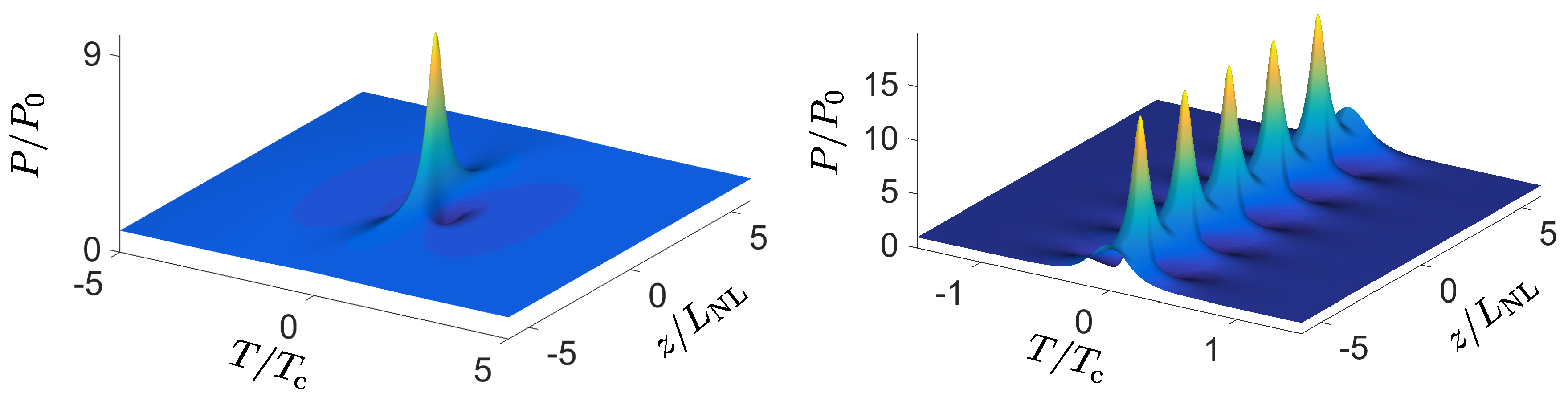
This is a structure that is localized in both time and space, known as the Peregrine soliton [20]. It is shown in Figure 5 (left); a first experimental demonstration was given in [21]. A further member of this family of NLSE solutions was studied in [22] and is known as the Kuznetsov–Ma soliton. Mathematically, that solution is described by the modulation term:
with a parameter range of . It consists of a periodically-recurring peak; see Figure 5 (right).
3. Extensions to the Nonlinear Schrödinger Equation
3.1. Generalized Nonlinear Schrödinger Equation
The NLSE neglects linear loss, approximates dispersion by the leading group velocity dispersion term and ignores nonlinear effects other than the intensity dependence of the refractive index. Depending on the situation and/or the required accuracy of the calculated results, terms must be added to include what is not represented. This leads to a generalized NLSE, which may take the form:
As the generalized NLSE is not integrable, it usually must be treated numerically. The impact of the new terms is as follows:
The dispersion curve can be written as a Taylor expansion around the carrier frequency ; the NLSE is written so that the term appears. All higher-order terms (shown here up to the fourth order) provide corrections that become relevant when either the pulse spectrum gets quite wide or when the carrier frequency is close to a zero-dispersion point (wavelength where passes through zero) of the fiber.
The ‘self-steepening’ term [1,23] results from the intensity dependence of the group velocity and leads to an asymmetry in the pulse shape. It can produce shifts in spectral and temporal positions even in the absence of the Raman term.
The Raman effect leads to a redistribution of spectral power to the advantage of the low-frequency slope of the pulse spectrum. A first study of the Raman gain in fibers was done by R. H. Stolen et al. [24]. The gain curve peaks at a frequency offset of ≈13 , but is nonzero all the way down to zero offset. As a result, the spectral ‘center of mass’ of a pulse is shifted to lower frequencies. This ‘redshift’ scales with the inverse fourth power of the pulse width [25]. The term expressing this in the NLSE is shown here in a simplified version, which contains the Raman response time . This model is valid for pulses being longer than ≈100 ; more accurate models are described in [26,27,28].
The loss term contains Beer’s loss coefficient ; the impact of the loss can be characterized by the characteristic loss length . As long as the loss is weak, i.e., , the equilibrium of dispersive and nonlinear effects that characterizes the soliton is only mildly perturbed. In that situation, the soliton can rearrange its shape: With the peak power drooping and the width increasing slightly, Equation (4) can still be approximately fulfilled even when the energy is reduced [29,30].
3.2. Dispersion-Managed Fibers
As a further complication in a realistic assessment of pulse propagation in fibers, one must acknowledge that in the telecommunications field, a special type of fiber has been preferred for 20 years now in which is not a constant. Originally, an attempt was made to cancel dispersive effects by concatenating segments of fiber with alternatingly positive and negative group velocity dispersion. As it turned out, a perfect cancellation (path average )—possible at a single wavelength only anyway—did not work as well as if a small negative value were left. This is on account of the fiber’s nonlinearity.
Figure 6 illustrates the structure of a dispersion-managed fiber (DM fiber). The dispersion map is described by the spatial period with which the alternating pattern is repeated [31]. Strictly speaking, the value of the nonlinearity coefficient will also alternate from one fiber segment to the other.
It is not immediately clear whether in a dispersion-managed (DM) fiber something like solitons can exist, as they are solutions of the NLSE for anomalous dispersion only. However, as it turned out, a type of pulse exists that is stabilized by nonlinearity [32,33,34,35,36,37]. These pulses were then called dispersion-managed (DM) solitons. Their shape is neither of the usual unchirped sech type, nor constant. Rather, it breathes over a full dispersion period so that after a full period, the shape in both the amplitude and phase profile is restored. An example of a DM soliton is shown in Figure 7.
Mathematically, dispersion management is captured by making fiber parameters z-dependent:
This modifies the NLSE into a non-integrable form so that it does not support solitons in the usual sense. Depending on the dispersion modulation strength (essentially, –), the DM soliton shape may be nearly sech-shaped or closer to a Gaussian [38]. In the strong modulation limit DM, solitons exhibit oscillating tails [38,39]. There is no closed analytical expression for it, but good approximations to its shape can be found by numerical procedures like that given in [40]. During propagation, a DM soliton suffers from continuous radiative loss, which may be weak, but nevertheless must lead to its eventual decay. Fortunately, for applications, the decay distance typically exceeds any practically relevant fiber length.
It was eventually understood that dispersion-management provides advantages over a constant-dispersion fiber. It suppresses four-wave mixing, a process occurring in a transmission system with many wavelength channels filled simultaneously with independent data streams, where it leads to cross-talk and, thus, errors. An extensive review of dispersion-management is given in [31].
3.3. Cases Involving Several Solitons
We mention a few more cases in which solitons or their compounds play a role and which have received attention in the research literature.
3.3.1. Soliton Molecules
In DM fibers, stable compounds of solitons exist, which have been called soliton molecules [41]. The alternating dispersion creates a rapid to-and-fro of the chirp of DM solitons and, thus, a varying mutual force. If two DM solitons are in a particular mutual separation, the net force is zero, and an equilibrium is obtained [42,43]. For larger separations, there is attraction, for smaller, repulsion: it is a stable equilibrium. Soliton molecules also exist for more than two DM solitons and have been discussed as information carriers in data transmission [44,45]. As it turns out, there can be several equilibrium positions [46].
3.3.2. Soliton Gas and Crystal
Another situation in which soliton propagation is subject to periodic perturbation was described in a series of experiments about a synchronously-driven fiber resonator [47] (using non-DM fiber). Free propagation in the fiber alternated with interference at an input coupler. As a result, relatively long input pulses organized themselves into a pattern that contained a multitude of short pulses; each of those fulfilled the soliton condition Equation (4). The pattern could be either chaotic (soliton gas) [48] or periodic (called soliton crystal) [49], depending on the drive power.
Similar phenomena have also been reported from fiber lasers [50,51,52], which, however, are not described by the NLSE, as that does not consider nonlinear gain and loss. An equation including these effects is the cubic-quintic complex Ginzburg–Landau equation. One finds that there are soliton-like solutions of this equation that are called dissipative solitons [53,54,55].
3.3.3. Supercontinuum Generation
For some metrological purposes like coherence tomography, wide bandwidth light with good focusability is required. Thermal light sources cannot deliver adequate power due to both their insufficient spatial coherence and the limitations set by Planck’s radiation law. One can, however, generate broadband light in a fiber by exploiting the nonlinearity to create new frequency components. Experiments involve, in most cases, a powerful mode-locked laser and a piece of highly nonlinear fiber. Either a modulation instability according to an Akhmediev breather scenario evolves, but the structure then breaks apart, or the input pulse represents a high-order () soliton, which undergoes fission [56]. In either event, the initial light signal breaks up into an arrangement of several pulses, many of which have soliton characteristics, and radiation. This arrangement has similarities to the soliton gas described above. Through the action of the Raman effect, four-wave mixing and cross-phase modulation combined with complex phase matching properties in the fiber’s dispersion curve (see, e.g., [57]), the light quickly develops a spectrum that may easily be one octave wide and often much more. Such a structure is referred to as an optical supercontinuum and has found much research interest; commercial supercontinuum sources are being offered. A good review is [58].
A corollary to this is the phenomenon of optical rogue waves. Rogue waves of the ocean have been identified as a real phenomenon, not a myth. Unusually, large single waves can occasionally appear without warning, possibly wreaking havoc on ships, and disappear again just as suddenly. It was first discussed in [59] that in the context of optical supercontinuum generation, single spikes of extreme power can occur every once in a while. There is an ongoing discussion about the mechanisms [60].
4. Methods to Verify Soliton Content
The inverse scattering technique allows one to find solutions to integrable nonlinear wave equations. However, in practice, one quite often is faced with the reversed task of determining the soliton content of a given signal. The task is relatively straightforward when the signal consists of isolated bell-shaped pulses. One can check whether the power profile approximates a shape and whether the chirp is close to zero. Then, duration and peak power can be checked with Equation (4). This way, an soliton can be directly identified, and for pulses with , the local value of N can be found. However, the applicability of this direct method is limited to simple cases. It is of no use for waveforms, as they may be found in more complex situations like soliton gas or optical supercontinuum; see Section 4.1.3.
We will therefore briefly describe more advanced techniques. The direct scattering method is often considered as the benchmark for the determination of soliton parameters. However, it has its limitations, chief among which is that it relies on the integrability of the system. An alternative is soliton radiation beat analysis, which does not have that same restriction, but the price to be paid for that is that (i) more input data are required and that (ii) in complex cases, the obtained pattern may get too complicated to interpret.
4.1. The Inverse and Direct Scattering Transform
4.1.1. The Method
The inverse scattering transform (IST) is a technique that can be used to solve certain nonlinear partial differential equations (PDE) like the Korteweg–de Vries equation, the sine-Gordon equation or the nonlinear Schrödinger equation. The basic concepts of this method were presented in 1967 in a groundbreaking paper by Gardner and coworkers dealing with the Korteweg–de Vries equation [5]. Shortly after, Lax showed how to apply the method also to other nonlinear PDEs when certain conditions are met [61]. The IST was successfully adapted to the NLSE by Zakharov and Shabat in 1972 [4].
The method of IST is based on transformations between the time-space domain and a nonlinear spectral domain, in which the nonlinear evolution of some given input field reduces to a linear problem. In the spectral domain, a given field is represented by its scattering spectrum, which is calculated by the so-called direct scattering transform (DST). The inverse operation is called the inverse scattering transform. As these transformations can be regarded as extensions to the well-known Fourier transform, they are also known as nonlinear Fourier transform and inverse nonlinear Fourier transform, respectively. Using the nonlinear Fourier transform, one can get insight into the linear and nonlinear components of a given field by analyzing its scattering spectrum. Generally, it consists of a continuous part, which represents the small amplitude radiation, and a discrete part, which can be attributed to the solitons contained.
In recent years, several groups took up the idea of using multi-soliton pulses for nonlinear optical data transmission, which originally was suggested by Hasegawa and Nyu [62]. In the course of this renewed attention, several nonlinear transmission schemes and techniques for the nonlinear Fourier transform and its inverse transform have been (and still are) developed to overcome the linear capacity limits of fiber-optical transmission lines. An overview about the latest developments can be found in [63].
DST is a great tool to analyze given pulses, but its application is somewhat involved. The DST has been applied analytically to only a few simple pulse shapes like sech-shaped [6] or rectangular pulses [64]. Even for such a standard shape as a Gaussian,
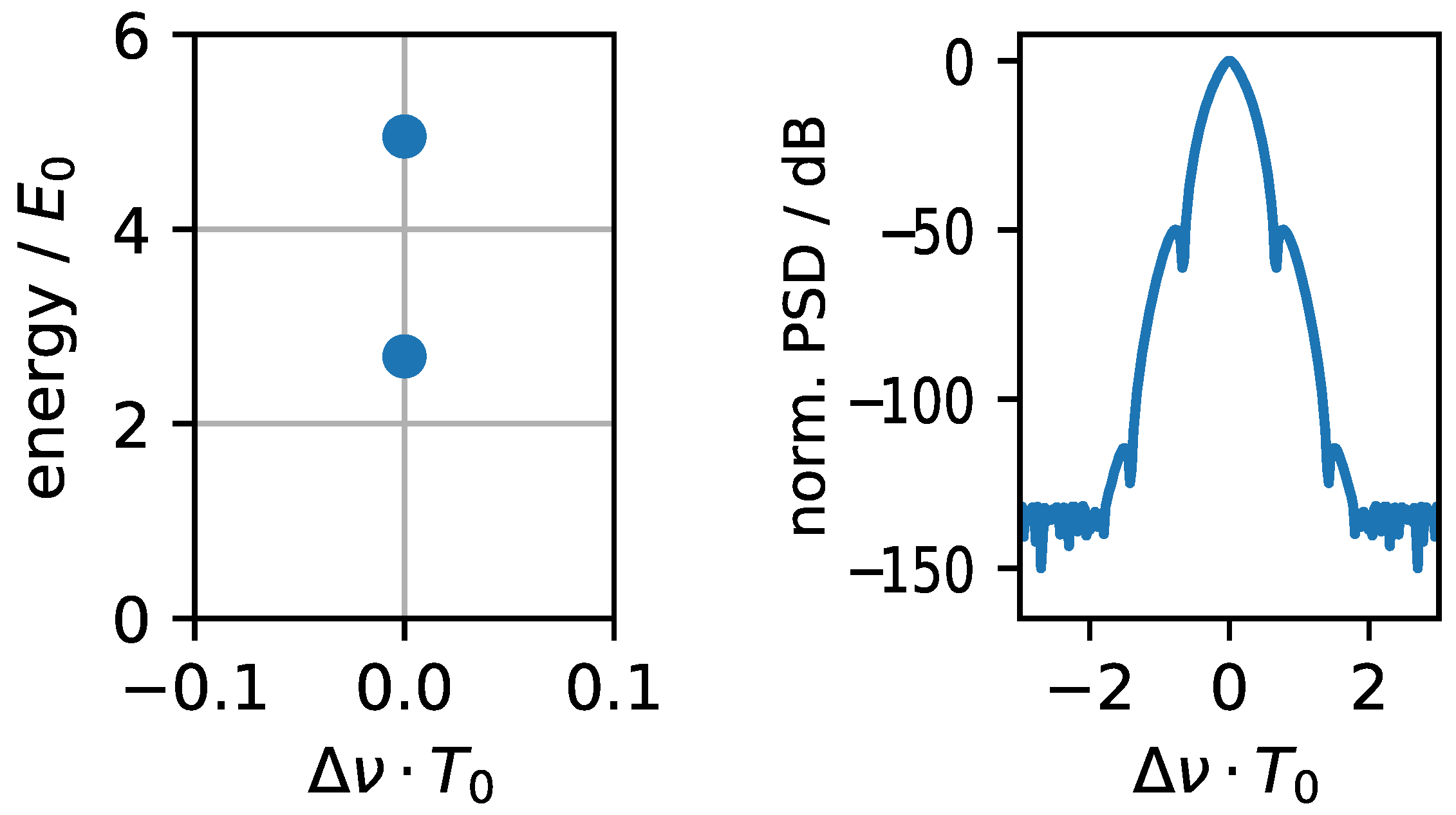
no analytical result is known to the authors’ best knowledge. Instead, approximate solutions can be found numerically. As an example, when setting and choosing and according to Equation (4), DST reveals that the pulse consists of two solitons and a small amplitude radiation part of nontrivial spectral shape (see Figure 8).
Various schemes for numerical calculations of the DST are available [63,65,66,67,68]. They all solve the Zakharov–Shabat eigenvalue problem of a discretized input field with M sample points and determine the nonlinear spectrum. One can distinguish between matrix methods that calculate the eigenvalues directly from a matrix and search methods in which the eigenvalues are found in an iterative manner. For a recent discussion, see, e.g., [63,66,67,68].
In the following, we will sketch briefly how to calculate the scattering spectrum using a search method. Using the formulation of Ablowitz et al. [69], one finds that solving the dimensionless NLSE:
is equivalent to the integration of the system of equations:
T and Z are operators (matrices) that determine the temporal and spatial evolution of some auxiliary function:
where and are called Jost functions. Explicitly, the operator T can be written as:
Calculation of the DST can be done by integrating Equation (20) with respect to time with different test values of the eigenvalue candidate . The initial condition can be chosen as:
when q is localized in the sense that for , at an exponential rate [65,66]. As a result, one obtains the scattering coefficients and from :
Additionally, the derivatives of a and b with respect to can also be calculated by extending the integration scheme to include .
In the scattering spectrum for anomalous dispersion, solitons are present in the form of discrete eigenvalues with and . represents the frequency, and corresponds to the amplitude of the soliton; both values are preserved during propagation. The continuous part of the spectrum (radiation) can be calculated from the values of , with . The spectral power density is then obtained as:
4.1.2. Numerical Restrictions
We have applied numerical DST to a case for which exact analytical results are known, i.e., the fundamental soliton Equation (3), to assess inaccuracies of the numerical procedure. They arise from various sources; we identify three main error sources.
Truncation error: At the edges of the computational time window of finite width , the pulse wings are truncated. A fraction of the energy is not represented in the numerical field:
Sampling error: Sampling error arises from coarse sampling when the temporal discretization step is too wide for the pulse duration.
Floating point error: Computers store numbers in some format with a limited number of digits; ‘double precision’ usually offers 15 digits plus the exponent. After a large number of floating point operations, numerical errors accumulate.
To disentangle these contributions, we varied the number of sampling points and the width of the time window for a given pulse width; the results are shown in Figure 9. To the right, the computational window is sufficiently wide (). Then, the three curves shown are for discretization step numbers as indicated by the labels. For points, sampling is increasingly coarse when these points are spread over a wider window, and the error rises. Larger numbers of points improve the situation quadratically because the error scales with the square of the sampling point separation. To the left, truncation error dominates; the prediction of Equation (28), plotted as a solid curve, fits well. Floating point error becomes relevant only where these two contributions are small and where the number of calculation steps is large; in our example, it appears as ‘noise’ in the central section of the curve for points. We convinced ourselves that the transfer-matrix (TM) method presented in [65] yields the same results.
4.1.3. Applications and Limitations of DST
The DST method as described so far is quite generally applicable to arbitrary pulse profiles provided two conditions are met: One is integrability, which is not fulfilled for many structures in the generalized NLSE in Section 3.1 and for DM systems in Section 3.2. The other is that for time to infinity, the structure must decay to zero sufficiently fast [65,66]. This is not the case for the structures described in Section 2.2.
If integrability is violated only weakly either by loss or through the Raman effect, the concept of solitons remains valid in an approximate sense as pulses that maintain an (near-) equilibrium between dispersive and nonlinear influences. It might be more accurate to speak then of solitary pulses. Strictly speaking, though, all preserved quantities are no more. Perturbation theory has shown [29,30] that solitons rearrange their shape in terms of width and peak power; in the process, they acquire a new energy value, as well. In the sense that this may still be interpreted as solitons, some researchers have adopted the following strategy: In a mildly non-integrable system with loss [70] or Raman effect [71,72,73], the pulse structure is propagated numerically up to some position , where DST is then applied to find what one may call ‘local eigenvalues’. Then, one lets slide and repeats DST, in order to find the position dependence, or spatial evolution, of the eigenvalues. An example of such a case is shown in Figure 10 where the Raman effect, third-order dispersion and loss are treated separately. The most conspicuous effects are the energy reduction by the loss term and the frequency downshift by the Raman effect.
When it comes to complex situations like in the context of optical supercontinuum generation where many interactions and collisions of several pulses take place, energy can be transferred between pulses, and more changes to local eigenvalues will occur. In any event, one has to interpret the results produced in this way with caution.
If one considers infinitely-extended structures, one first needs to acknowledge that they have infinite energy. One possible approach is to start with a finite piece (‘window’) of the infinite structure and determine eigenvalues, then increment the window width and follow the eigenvalues; finally, let the window width tend to infinity [74]. In the limit, one obtains an infinite number of eigenvalues, but with a finite density (number of eigenvalues per unit time). These eigenvalues cover a continuum of energies from zero up to some maximum; if one considers the simplest case of an unmodulated continuous wave, this maximum depends only on its power and is given by . With respect to the interpretation of these eigenvalues as signatures of solitons, the following was shown in [74]: Consider a finite window, which contains m eigenvalues, and allow it to propagate. On account of integrability, it contains a constant number of m solitons. If one then applies a perturbation, e.g., by Raman effect, precisely m separate pulses emerge; once they are sufficiently separated from each other after some propagation, it can be checked that each fulfills the soliton criterion Equation (4).
The other approach to infinitely extended fields is to consider periodic problems, like the Akhmediev breather. Adaptations of IST to periodic boundary conditions (periodic IST, also called finite gap theory) have been given in [75,76,77] where the obtained eigenvalues are not necessarily interpreted as solitons, but rather as the representation of linear and nonlinear modes [78,79,80]. Like the nonperiodic IST, this periodic case gained renewed interest in recent years. Different theoretical and numerical schemes have been developed with a view toward the application of nonlinear data transmission [63,66,67,81,82,83]. A variant of the periodic DST based on the artificial periodization of field components was used to analyze rogue events and numerically to find the eigenvalue spectra of the breather solutions of Section 2.2 [84]. Another approach to characterize rogue events via DST was taken in [85,86].
We have here concentrated on pulse-like initial conditions. Recently, the scope was extended to integrable turbulence [87] with a view towards understanding rogue waves. Initial conditions for the NLSE were generated by superimposing random perturbations in both amplitude and phase on a continuous wave; the resulting field was characterized by its eigenvalue spectrum.
4.2. Soliton Radiation Beat Analysis
Soliton radiation beat analysis (SRBA) is a numerical method to determine the soliton content of a pulse in an optical fiber even if the system is not integrable. In contrast to DST, which requires the pulse profile at a single position in the fiber, SRBA requires knowledge of the evolution over a certain length section of the fiber. This is easily understood: In integrable systems, soliton parameters are invariant so that if they are known in one place, they are known everywhere. SRBA can follow the evolution of soliton parameters in a non-integrable setting; the price to pay is that representative information about it must be introduced into the calculation.
As early as in 1974, it was noted [6] that the envelope of a pulse not exactly conforming to a soliton undergoes oscillations. Such a pulse contains a soliton and some radiation; the oscillation arises as a beating between both. The radiation evolves linearly; the soliton contains a power-dependent phase term as shown in Equation (3). The frequency of the beat note therefore allows a direct conclusion about the soliton energy.
The SRBA method was first introduced in [88]. The propagation of a sech pulse with the initial form was simulated numerically. This was repeated while incrementing the soliton parameter N. As the oscillation of the peak power is damped due to dispersive spreading of the radiative part, it was found advantageous to evaluate the peak spectral power, which undergoes undamped oscillation. A windowed Fourier transform was applied to the spatial evolution of the power at the center frequency . This produces a spectrogram of spatial frequencies called the soliton radiation beat pattern. An example is shown in Figure 11 (left).
As N is increased, a soliton radiation beat first appears at its expected threshold near . The figure shows that this beat note also has overtones. Its amplitude (grey scale) vanishes at integer N (apparent ‘white stripes’), which is of course because there, the radiation amplitude vanishes; the beat amplitude is proportional to the product of both amplitudes.
If there is more than one soliton involved, the beat pattern will contain the frequencies of beats between all pairs of solitons, as well as that of each soliton beating with radiation. In Figure 11 (left), traces pertaining to the second soliton begin at as expected and have amplitude nulls at . Difference frequencies are visible as downward-bending curves. In the right panel of Figure 11, analytical results for beat frequencies are plotted for comparison. Shown are all calculated frequencies, up to four overtones, and all combination frequencies of this multitude. It is obvious that all SRBA traces of the left panel can be identified in this way. SRBA provides the additional information that there are notches in the amplitudes of all traces involving radiation at integer N values.
This shows that SRBA reproduces all known features of the soliton energies as known analytically from IST. In [89], this method was shown to work for chirped Gaussian pulses in the NLSE. Going beyond the NLSE to non-integrable situations is also possible as SRBA makes no assumption about integrability. A lossy fiber was treated in [90]. It was shown that a mild, ‘adiabatic’ loss, if it persists for a long fiber length, eventually turns diabatic because the relevant length scales and also change in the process. Once the loss is diabatic, the soliton decays. In that situation, however, the applicability of DST even in the approximate sense as described above in Section 4.1.3 is ultimately lost, and interpretations based on that approach [70] are doubtful and at variance to the SRBA results.
A further important example of the application of SRBA is the determination of the dispersion-managed soliton content. This case is just not accessible for DST, not even in the sense of ‘local’ analysis as in Section 4.1.3. Other than SRBA, no other numerical method to analyze DM structures is known. In [88], a suitably-scaled Gaussian pulse was used as a good approximation to an ideal DM soliton, and an SRBA pattern was obtained. Both the modification of the soliton energy and the characteristic minima of soliton radiation beat traces were found.
In subsequent research, SRBA was also applied to analyze Akhmediev breathers and a sinusoidally modulated cw [91], as well as soliton crystals [92]. One can assume that in principle, the SRBA method can be applied to all non-integrable systems where a nonlinear phase shift appears. Potential applications are soliton molecules (see Section 3.3.1) or dissipative solitons (see Section 3.3.2).
SRBA as described so far relies on the evaluation of the central spectral power . In a generalization of the technique, the consideration is extended to the full spectrum, [93]. In this variant, the technique also yields information about soliton velocities. Figure 12 shows an example for the case of an soliton.
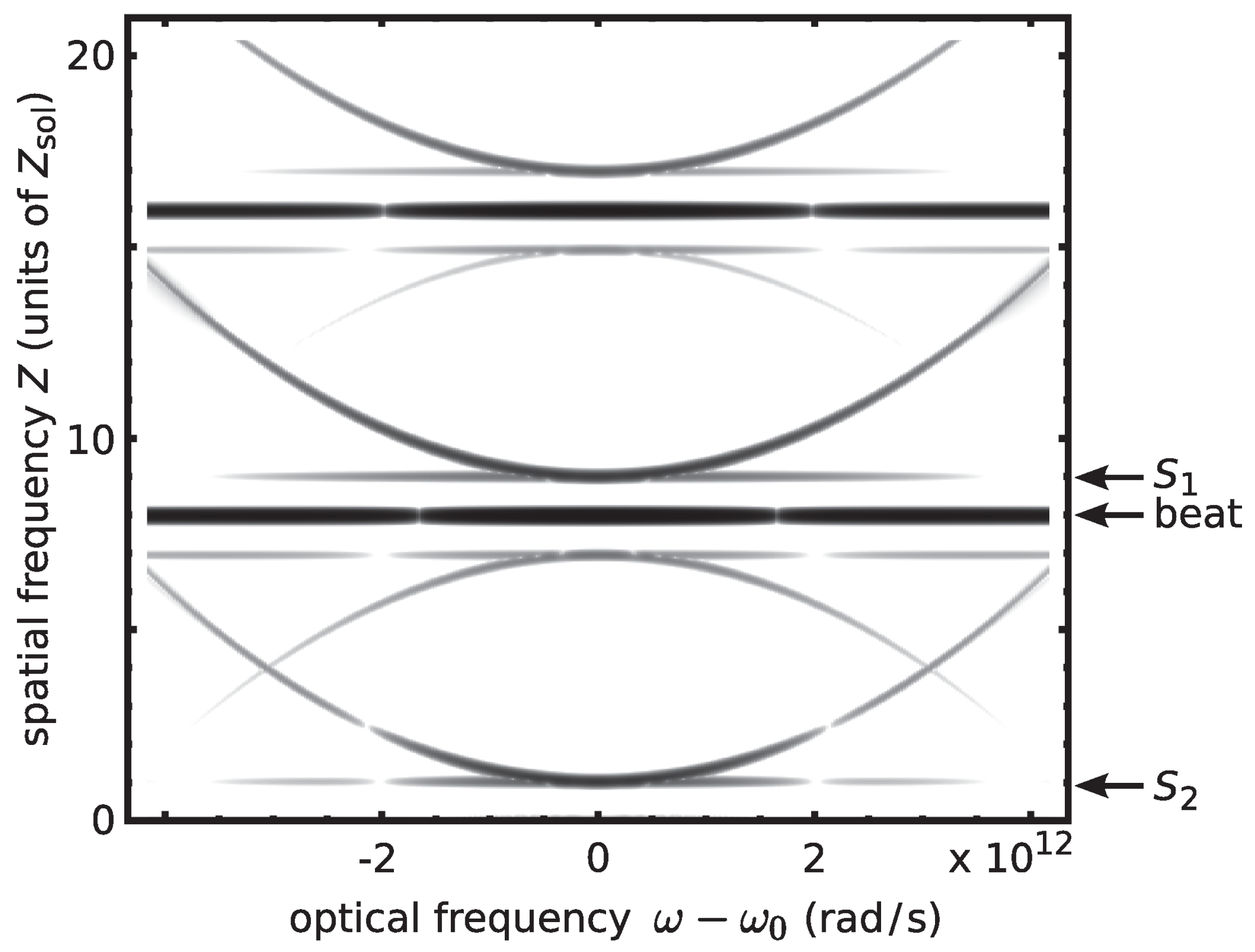
The pattern was generated using a value of , so that there is always a little bit of radiation copropagating with the second-order soliton, and a beat note is generated. Parabola-like curves are due to radiation; horizontal flat lines touching the parabolas are due to solitons. Once the traces are identified, the soliton energies can be obtained from the spatial frequency of the nonlinear phase rotation. To illustrate the interpretation of such data, we point out that the two solitons appear with spatial frequencies in the ratio of 9:1. According to Equation (3), this means that the peak powers are . Equation (4) then dictates that . The ratio of energies obtained from Equation (5) is then 3:1, precisely as expected from Figure 3. Any frequency shifts would appear as horizontal displacements; in this particular example, there are none. There is no scan of N here; this extended procedure has the advantage that only a single propagation simulation is necessary.
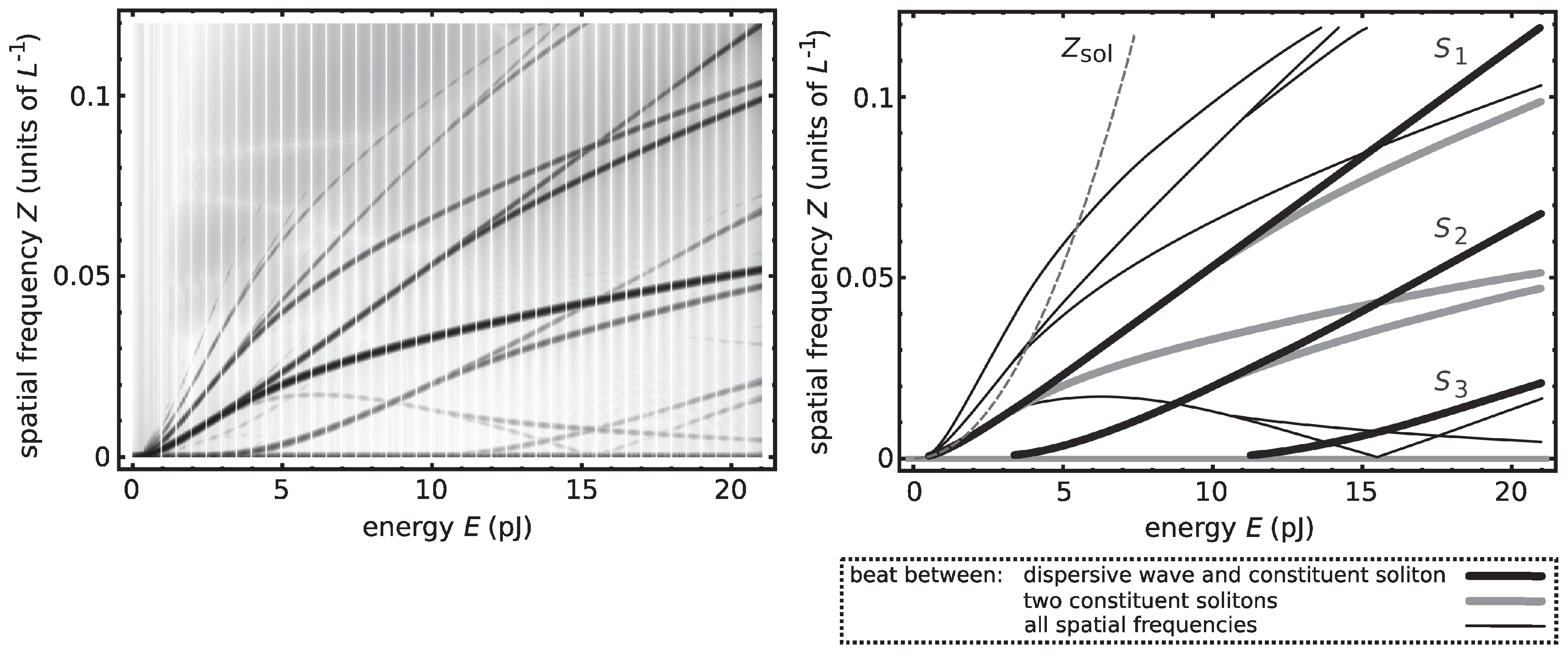
A particular difficulty with DM solitons is that their shape undergoes continuous changes. At various positions within , the shape varies considerably, but the pulse shape repeats after (it is ‘stroboscopically’ stable). Even then, when the power is modified, the shape varies from ‘nearly sech’ to ‘nearly Gaussian’, and depending on the dispersion modulation depth, oscillating tails may appear. Therefore, extra measures need to be taken when the energy is scanned for an SRBA pattern calculation. For the data in the left panel of Figure 13, at 0.5 pJ increments of energy, the best approximation to the DM soliton shape was found using Nijhof’s method [40]. If the pulse shape were exact, there would be no beat note with radiation. This is why in 0.5 pJ increments, there seem to be white lines in the figure. Above and below each such step, the energy was scanned by simple scaling of the pulse shape to . The slight deviation from the best pulse shape suffices to produce beat notes, and a full survey of their positions is obtained. For better clarity, the data from this calculation are transferred to the right panel of Figure 13, and different line thicknesses are standardized into three classes in the process. The data show that a DM soliton consists of several constituent solitons; the pertaining traces are labeled –.
A comparison of DST and SRBA reveals the advantages and weaknesses of both. SRBA requires more input data. These can only be available from numerical simulations; it is hard to imagine how suitable data could be obtained from an experiment. On the other hand, SRBA can treat cases that are inaccessible to DST. Its limit is reached when for a growing number of solitons involved, the number of traces becomes too large to disentangle them all. DST can be applied to many-soliton cases [94], but only in strictly integrable systems, or with the limitations in ‘nearly integrable’ systems as pointed out in Section 4.1.3.
5. Conclusions
Solitons in optical fibers are pulses of light that maintain a balance between linear and nonlinear distortions. Real-world systems are rarely, if ever, of the integrable kind. It is therefore appropriate to apply the word ‘soliton’ also to pulses for which the balance is maintained at least approximately; to do so is now common usage. However, one occasionally sees research papers in which the word is used in a very loose sense, with no effort being made to actually check whether the balance is fulfilled.
In this review, we outline the concept of fiber-optic solitons, with a particular view toward methods of verification of the solitonic nature of a given pulse, or group of pulses, or a similar structure. Soliton content has been discussed in the context of structures like soliton molecules, soliton gas and crystal, Akhmediev breather, optical supercontinuum and rogue waves. The simplest method is to check pulse parameters with Equation (4), which directly expresses an equilibrium condition. Unfortunately, this straightforward test is only applicable in very simple situations when there are clean, well-isolated pulses, and it does not fully quantify the soliton content. Grown from inverse scattering theory, the first method to analytically find the soliton solution of the NLSE is direct scattering transform. It basically tests whether the structure under test contains pulses that hang together as entities even when they collide, the property that gave solitons their ‘particle-like’ name [95]. An alternative method is soliton radiation beat analysis, which basically tracks the nonlinear phase rotation, which is the signature of solitons. We discuss some issues of practicality and accuracy and compare the ranges of applicability of both DST and SRBA.
There is no single method that covers all cases; indeed, in some relevant cases, no available method is fully satisfactory. In the complex evolution of supercontinuum, for example, the method is often adapted ad hoc to the situation, for want of alternatives. In some interesting cases, soliton content analysis has not been pursued yet, to our knowledge. Dissipative solitons are subject to yet another condition beyond Equation (4), but should be accessible for SRBA. This article is meant to provide the reader with a survey to what is currently known, to foster future research.
Author Contributions
F.M., C.M. and A.H.have contributed equally to this manuscript.
Conflicts of Interest
The authors declare no conflict of interest.
Abbreviations
The following abbreviations are used in this manuscript:
| cw | continuous wave |
| DM | dispersion-management |
| DST | direct scattering transform |
| IST | inverse scattering transform |
| NLSE | nonlinear Schrödinger equation |
| SRBA | soliton radiation beat analysis |
References
- Agrawal, G.P. Nonlinear Fiber Optics, 5th ed.; Academic Press: Oxford, UK, 2013. [Google Scholar]
- Mitschke, F. Fiber Optics. Physics and Technology, 2nd ed.; Springer: Heidelberg, Germany, 2016. [Google Scholar]
- Stolen, R.H.; Lin, C. Self-phase-modulation in silica optical fibers. Phys. Rev. A 1978, 17, 1448–1453. [Google Scholar] [CrossRef]
- Zakharov, V.E.; Shabat, A.B. Exact Theory of Two-Dimensional Self-Focusing and One-Dimensional Self-Modulation of Waves in Nonlinear Media. Sov. Phys. JETP 1972, 34, 62–69. [Google Scholar]
- Gardner, C.S.; Greene, J.M.; Kruskal, M.D.; Miura, R.M. Method for Solving the Korteweg-de Vries Equation. Phys. Rev. Lett. 1967, 19, 1095–1097. [Google Scholar] [CrossRef]
- Satsuma, J.; Yajima, N. Initial Value Problem of One-Dimensional Self-Modulation of Nonlinear Waves in Dispersive Media. Prog. Theor. Phys. Suppl. 1974, 55, 284–306. [Google Scholar] [CrossRef]
- Hasegawa, A.; Tappert, F. Transmission of stationary nonlinear optical pulses in dispersive dielectric fibers. I. Anomalous dispersion. Appl. Phys. Lett. 1973, 23, 142–144. [Google Scholar] [CrossRef]
- Mollenauer, L.F.; Stolen, R.H.; Gordon, J.P. Experimental Observation of Picosecond Pulse Narrowing and Solitons in Optical Fibers. Phys. Rev. Lett. 1980, 45, 1095–1098. [Google Scholar] [CrossRef]
- Yang, J. Nonlinear Waves in Integrable and Nonintegrable Systems; Society for Industrial and Applied Mathematics (SIAM): Philadelphia, PA, USA, 2010. [Google Scholar]
- Kivshar, Y.S.; Agrawal, G.P. Optical Solitons. From Fibers to Photonic Crystals; Academic Press: London, UK, 2003. [Google Scholar]
- Schrader, D. Explicit calculation of N-Soliton Solutions of the nonlinear Schrödinger equation. IEEE J. Quantum Electron. 1995, 31, 2221–2225. [Google Scholar] [CrossRef]
- Gordon, J.P. Interaction forces among solitons in optical fibers. Opt. Lett. 1983, 8, 596–598. [Google Scholar] [CrossRef] [PubMed]
- Mitschke, F.; Mollenauer, L.F. Experimental observation of interaction forces between solitons in optical fibers. Opt. Lett. 1987, 12, 355–357. [Google Scholar] [CrossRef] [PubMed]
- Desem, C.; Chu, P.L. Reducing soliton interaction in single-mode optical fibres. IEEE Proc. 1987, 134, 145–151. [Google Scholar] [CrossRef]
- Akhmediev, N.N.; Korneev, V.I. Modulation instability and periodic solutions of the nonlinear Schrödinger equation. Theor. Math. Phys. 1986, 69, 1089–1093. [Google Scholar] [CrossRef]
- Mahnke, C.; Mitschke, F. Ultrashort Light Pulses Generated from Modulation Instability: Background Removal and Soliton Content. Appl. Phys. B 2013, 116, 15–20. [Google Scholar] [CrossRef]
- Dudley, J.M.; Genty, G.; Dias, F.; Kibler, B.; Akhmediev, N. Modulation instability, Akhmediev Breathers and continuous wave supercontinuum generation. Opt. Express 2009, 17, 21497–21508. [Google Scholar] [CrossRef] [PubMed]
- Hammani, K.; Wetzel, B.; Kibler, B.; Fatome, J.; Finot, C.; Millot, G.; Akhmediev, N.; Dudley, J.M. Spectral dynamics of modulation instability described using Akhmediev breather theory. Opt. Lett. 2011, 36, 2140–2142. [Google Scholar] [CrossRef] [PubMed]
- Hasegawa, A. Generation of a train of soliton pulses by induced modulational instability in optical fibers. Opt. Lett. 1984, 9, 288–290. [Google Scholar] [CrossRef] [PubMed]
- Peregrine, D.H. Water waves, nonlinear Schrödinger equations and their solutions. J. Aust. Math. Soc. B 1983, 25, 16–43. [Google Scholar] [CrossRef]
- Kibler, B.; Fatome, J.; Finot, C.; Dias, F.; Genty, G.; Akhmediev, N.; Dudley, J.M. The Peregrine soliton in nonlinear fiber optics. Nat. Phys. 2010, 6, 790–795. [Google Scholar] [CrossRef]
- Kibler, B.; Fatome, J.; Finot, C.; Millot, G.; Genty, G.; Wetzel, B.; Akhmediev, N.; Dias, F.; Dudley, J.M. Observation of the Kuznetsov-Ma soliton dynamics in optical fibre. Sci. Rep. 2012, 2, 463. [Google Scholar] [CrossRef] [PubMed]
- Anderson, D.; Lisak, M. Nonlinear asymmetric self-phase modulation and self-steepening of pulses in long optical waveguides. Phys. Rev. A 1983, 27, 1393–1398. [Google Scholar] [CrossRef]
- Stolen, R.H.; Lee, C.; Jain, R.K. Development of the stimulated Raman spectrum in single-mode silica fibers. J. Opt. Soc. Am. B 1984, 1, 652–657. [Google Scholar] [CrossRef]
- Gordon, J.P. Theory of the soliton self frequency shift. Opt. Lett. 1986, 11, 662–664. [Google Scholar] [CrossRef] [PubMed]
- Stolen, R.H.; Gordon, J.P.; Tomlinson, W.J.; Haus, H.A. Raman response function of silica-core fibers. J. Opt. Soc. Am. B 1989, 6, 1159–1166. [Google Scholar] [CrossRef]
- Mamyshev, P.V.; Chernikov, S.V. Ultrashort-pulse propagation in optical fibers. Opt. Lett. 1990, 15, 1076–1078. [Google Scholar] [CrossRef] [PubMed]
- Lin, Q.; Agrawal, G.P. Raman response function for silica fibers. Opt. Lett. 2006, 31, 3086–3088. [Google Scholar] [CrossRef] [PubMed]
- Kaup, D.J. A perturbation expansion for the Zakharov–Shabat inverse scattering transform. SIAM J. Appl. Math. 1976, 31, 121–133. [Google Scholar] [CrossRef]
- Hasegawa, A.; Kodama, Y. Amplification and reshaping of optical solitons in a glass fiber—I. Opt. Lett. 1982, 7, 285–287. [Google Scholar] [CrossRef] [PubMed]
- Turitsyn, S.K.; Bale, B.G.; Fedoruk, M.P. Dispersion-managed solitons in fibre systems and lasers. Phys. Rep. 2012, 521, 135–203. [Google Scholar] [CrossRef]
- Smith, N.J.; Knox, F.M.; Doran, N.J.; Blow, K.J.; Bennion, I. Enhanced power solitons in optical fibres with periodic dispersion management. Electron. Lett. 1996, 32, 54–55. [Google Scholar] [CrossRef]
- Nijhof, J.H.B.; Doran, N.J.; Forysiak, W.; Knox, F.M. Stable soliton-like propagation in dispersion managed systems with net anomalous, zero and normal dispersion. Electron. Lett. 1997, 33, 1726–1727. [Google Scholar] [CrossRef]
- Chen, Y.; Haus, H.A. Dispersion-managed solitons with net positive dispersion. Opt. Lett. 1998, 23, 1013–1015. [Google Scholar] [CrossRef] [PubMed]
- Turytsin, S.K.; Shapiro, E.G. Dispersion-managed solitons in optical amplifier transmission systems with zero average dispersion. Opt. Lett. 1998, 23, 682–684. [Google Scholar] [CrossRef]
- Kutz, J.N.; Evangelides, S.G. Dispersion-managed breathers with average normal dispersion. Opt. Lett. 1998, 23, 685–687. [Google Scholar] [CrossRef] [PubMed]
- Grigoryan, V.S.; Menyuk, C.R. Dispersion-managed solitons at normal average dispersion. Opt. Lett. 1998, 23, 609–611. [Google Scholar] [CrossRef] [PubMed]
- Turitsyn, S.; Shapiro, E.; Medvedev, S.; Fedoruk, M.P.; Mezentsev, V. Physics and mathematics of dispersion managed optical solitons. C. R. Phys. 2003, 4, 145–161. [Google Scholar] [CrossRef]
- Lushnikov, P.M. Oscillating tails of a dispersion-managed soliton. J. Opt. Soc. Am. B 2004, 21, 1913–1918. [Google Scholar] [CrossRef]
- Nijhof, J.H.B.; Forysiak, W.; Doran, N.J. The averaging method for finding exactly periodic dispersion-managed solitons. IEEE J. Sel. Top. Quantum Electron. 2000, 5, 330–336. [Google Scholar] [CrossRef]
- Stratmann, M.; Pagel, T.; Mitschke, F. Experimental Observation of Temporal Soliton Molecules. Phys. Rev. Lett. 2005, 95, 143902. [Google Scholar] [CrossRef] [PubMed]
- Hause, A.; Hartwig, H.; Seifert, B.; Stolz, H.; Böhm, M.; Mitschke, F. Phase structure of soliton molecules. Phys. Rev. A 2007, 75, 063836. [Google Scholar] [CrossRef]
- Hause, A.; Hartwig, H.; Böhm, M.; Mitschke, F. Binding mechanism of temporal soliton molecules. Phys. Rev. A 2008, 78, 063817. [Google Scholar] [CrossRef]
- Rohrmann, P.; Hause, A.; Mitschke, F. Solitons Beyond Binary: Possibility of Fibre-Optic Transmission of Two Bits per Clock Period. Sci. Rep. 2012, 2, 866. [Google Scholar] [CrossRef] [PubMed]
- Rohrmann, P.; Hause, A.; Mitschke, F. Two-soliton and three-soliton molecules in optical fibers. Phys. Rev. A 2013, 87, 043834. [Google Scholar] [CrossRef]
- Hause, A.; Mitschke, F. Higher-order equilibria of temporal soliton molecules in dispersion-managed fibers. Phys. Rev. A 2013, 88, 063843. [Google Scholar] [CrossRef]
- Steinmeyer, G.; Buchholz, A.; Hänsel, M.; Heuer, M.; Schwache, A.; Mitschke, F. Dynamical pulse shaping in a nonlinear resonator. Phys. Rev. A 1995, 52, 830–838. [Google Scholar] [CrossRef] [PubMed]
- Schwache, A.; Mitschke, F. Properties of an optical soliton gas. Phys. Rev. E 1997, 55, 7720–7725. [Google Scholar] [CrossRef]
- Malomed, B.A.; Schwache, A.; Mitschke, F. Soliton lattice and gas in passive fiber-ring resonators. Fiber Integr. Opt. 1998, 17, 267–277. [Google Scholar]
- Amrani, F.; Haboucha, A.; Salhi, M.; Leblond, H.; Komarov, A.; Sanchez, F. Dissipative solitons compounds in a fiber laser. Analogy with the states of the matter. Appl. Phys. B 2010, 99, 107–114. [Google Scholar] [CrossRef]
- Grelu, P.; Soto-Crespo, J.M. Temporal soliton “molecules” in mode-locked lasers: Collisions, pulsations, and vibrations. In Dissipative Solitons: From Optics to Biology and Medicine; Lecture Notes in Physics; Akhmediev, N., Ankiewicz, A., Eds.; Springer: Berlin/Heidelberg, Germany, 2008; Volume 751, pp. 137–173. [Google Scholar]
- Chouli, S.; Grelu, P. Soliton rains in a fiber laser: An experimental study. Phys. Rev. A 2010, 81, 063829. [Google Scholar] [CrossRef]
- Soto-Crespo, J.M.; Akhmediev, N.N.; Afanasjev, V.V. Stability of the pulselike solutions of the quintic complex Ginzburg–Landau equation. J. Opt. Soc. Am. B 1996, 13, 1439–1449. [Google Scholar] [CrossRef]
- Grelu, P.; Akhmediev, N.N. Dissipative solitons for mode-locked lasers. Nat. Photonics 2012, 6, 84–92. [Google Scholar] [CrossRef]
- Akhmediev, N.; Ankiewicz, A. (Eds.) Dissipative Solitons: From Optics to Biology and Medicine; Lecture Notes in Physics; Springer: Berlin/Heidelberg, Germany, 2008; Volume 751. [Google Scholar]
- Husakou, A.V.; Herrmann, J. Supercontinuum generation of higher-order solitons by fission in photonic crystal fibers. Phys. Rev. Lett. 2001, 87, 203901. [Google Scholar] [CrossRef] [PubMed]
- Roy, S.; Bhadra, S.K.; Agrawal, G.P. Perturbation of higher-order solitons by fourth-order dispersion in optical fibers. Opt. Commun. 2009, 282, 3798–3803. [Google Scholar] [CrossRef]
- Dudley, J.M.; Genty, G.; Coen, S. Supercontinuum generation in photonic crystal fiber. Rev. Mod. Phys. 2006, 78, 1135–1184. [Google Scholar] [CrossRef]
- Solli, D.R.; Ropers, C.; Koonath, P.; Jalali, B. Optical Rogue Waves. Nature 2007, 450, 1054–1057. [Google Scholar] [CrossRef] [PubMed]
- Akhmediev, N.; Kibler, B.; Baronio, F.; Belić, M.; Zhong, W.P.; Zhang, Y.; Chang, W.; Soto-Crespo, J.M.; Vouzas, P.; Grelu, P.; et al. Roadmap on optical rogue waves and extreme events. J. Opt. 2016, 18, 063001. [Google Scholar] [CrossRef]
- Lax, P.D. Integrals of nonlinear equations of evolution and solitary waves. Commun. Pure Appl. Math. 1968, 21, 467–490. [Google Scholar] [CrossRef]
- Hasegawa, A.; Nyu, T. Eigenvalue communication. J. Lightwave Technol. 1993, 11, 395–399. [Google Scholar] [CrossRef]
- Turitsyn, S.K.; Prilepsky, J.E.; Le, S.T.; Wahls, S.; Frumin, L.L.; Kamalian, M.; Derevyanko, S.A. Nonlinear Fourier transform for optical data processing and transmission: Advances and perspectives. Optica 2017, 4, 307–322. [Google Scholar] [CrossRef]
- Manakov, S.V. Nonlinear Fraunhofer diffraction. Zh. Eksp. Teor. Fiz. 1973, 65, 1392–1398. [Google Scholar]
- Boffetta, G.; Osborne, A. Computation of the Direct Scattering Transform for the Nonlinear Schroedinger Equation. J. Comput. Phys. 1992, 102, 252–264. [Google Scholar] [CrossRef]
- Kamalian, M.; Prilepsky, J.E.; Le, S.T.; Turitsyn, S.K. Periodic nonlinear Fourier transform for fiber-optic communications, Part I: Theory and numerical methods. Opt. Express 2016, 24, 18353–18369. [Google Scholar] [CrossRef] [PubMed]
- Kamalian, M.; Prilepsky, J.E.; Le, S.T.; Turitsyn, S.K. Periodic nonlinear Fourier transform for fiber-optic communications, Part II: Eigenvalue communication. Opt. Express 2016, 24, 18370–18381. [Google Scholar] [CrossRef] [PubMed]
- Yousefi, M.I.; Kschischang, F.R. Information transmission using the nonlinear Fourier transform, Part II: Numerical methods. IEEE Trans. Inf. Theory 2014, 60, 4329–4345. [Google Scholar] [CrossRef]
- Ablowitz, M.J.; Kaup, D.J.; Newell, A.C.; Segur, H. Nonlinear-Evolution Equations of Physical Significance. Phys. Rev. Lett. 1973, 31, 125–127. [Google Scholar] [CrossRef]
- Prilepsky, J.E.; Derevyanko, S.A. Breakup of a multisoliton state of the linearly damped nonlinear Schrödinger equation. Phys. Rev. E 2007, 75, 036616. [Google Scholar] [CrossRef] [PubMed]
- Kodama, Y.; Hasegawa, A. Nonlinear pulse propagation in a monomode dielectric guide. IEEE J. Quantum Electron. 1987, 23, 510–524. [Google Scholar] [CrossRef]
- Tai, K.; Bekki, N.; Hasegawa, A. Fission of optical solitons induced by stimulated Raman effect. Opt. Lett. 1988, 13, 392–394. [Google Scholar] [CrossRef] [PubMed]
- Gölles, M.; Uzunov, I.M.; Lederer, F. Break up of N-soliton bound states due to intrapulse Raman scattering and third-order dispersion—An eigenvalue analysis. Phys. Lett. A 1997, 231, 195–200. [Google Scholar] [CrossRef]
- Mahnke, C.; Mitschke, F. Possibility of an Akhmediev breather decaying into solitons. Phys. Rev. A 2012, 82, 033808. [Google Scholar] [CrossRef]
- Its, A.R.; Matveev, V.B. Schrödinger operators with finite-gap spectrum and N-soliton solutions of the Korteweg—de Vries equation. Theor. Math. Phys. 1975, 23, 51–68. [Google Scholar] [CrossRef]
- Kawata, T.; Inoue, H. Inverse scattering method for the nonlinear evolution equations under nonvanishing conditions. J. Phys. Soc. Jpn. 1978, 44, 1722–1729. [Google Scholar] [CrossRef]
- Ma, Y.C.; Ablowitz, M.J. The periodic cubic Schrodinger equation. Stud. Appl. Math. 1981, 65, 113–158. [Google Scholar] [CrossRef]
- Ma, Y.C. The Perturbed Plane Wave Solutions of the Cubic Schrödinger Equation. Stud. Appl. Math. 1979, 60, 43–58. [Google Scholar] [CrossRef]
- Tracy, E.R.; Chen, H.H. Nonlinear self-modulation: An exactly solvable model. Phys. Rev. A 1988, 37, 815–839. [Google Scholar] [CrossRef]
- Osborne, A. Nonlinear Ocean Waves and the Inverse Scattering Transform; International Geophysics Series; Academic Press: Burlington, MA, USA, 2010; Volume 97. [Google Scholar]
- Olivier, C.P.; Herbst, B.M.; Molchan, M.A. A numerical study of the large-period limit of a Zakharov–Shabat eigenvalue problem with periodic potentials. J. Phys. A Math. Theor. 2012, 45, 255205–255211. [Google Scholar] [CrossRef]
- Wahls, S.; Poor, H.V. Introducing the fast nonlinear Fourier transform. In Proceedings of the 2013 IEEE International Conference on Acoustics, Speech and Signal Processing (ICASSP), Vancouver, BC, Canada, 26–31 May 2013. [Google Scholar]
- Wahls, S.; Poor, H.V. Fast numerical nonlinear Fourier transforms. IEEE Trans. Inf. Theory 2015, 61, 6957–6974. [Google Scholar] [CrossRef]
- Randoux, S.; Suret, P.; El, G. Inverse scattering transform analysis of rogue waves using local periodization procedure. Sci. Rep. 2016, 6, 29238. [Google Scholar] [CrossRef] [PubMed]
- Weerasekara, G.; Tokunaga, A.; Terauchi, H.; Eberhard, M.; Maruta, A. Soliton’s eigenvalue based analysis on the generation mechanism of rogue wave phenomenon in optical fibers exhibiting weak third order dispersion. Opt. Express 2015, 23, 143–153. [Google Scholar] [CrossRef] [PubMed]
- Weerasekara, G.; Maruta, A. Characterization of optical rogue wave based on solitons’ eigenvalues of the integrable higher-order nonlinear Schrödinger equation. Opt. Commun. 2017, 382, 639–645. [Google Scholar] [CrossRef]
- Akhmediev, N.; Soto-Crespo, J.M.; Devine, N. Breather turbulence versus soliton turbulence: Rogue waves, probability density functions, and spectral features. Phys. Rev. E 2016, 94, 022212. [Google Scholar] [CrossRef] [PubMed]
- Böhm, M.; Mitschke, F. Soliton radiation beat analysis. Phys. Rev. E 2006, 73, 066615. [Google Scholar] [CrossRef] [PubMed]
- Böhm, M.; Mitschke, F. Soliton content of arbitrarily shaped light pulses in fibers analysed using a soliton-radiation beat pattern. Appl. Phys. B 2007, 86, 407–411. [Google Scholar] [CrossRef]
- Böhm, M.; Mitschke, F. Solitons in lossy fibers. Phys. Rev. A 2007, 76, 063822. [Google Scholar] [CrossRef]
- Zajnulina, M.; Böhm, M.; Blow, K.; Rieznik, A.A.; Giannone, D.; Haynes, R.; Roth, M.M. Soliton radiation beat analysis of optical pulses generated from two continuous-wave lasers. Chaos 2015, 25, 103104. [Google Scholar] [CrossRef] [PubMed]
- Zajnulina, M.; Böhm, M.; Bodenmüller, D.; Blow, K.; Chavez Boggio, J.M.; Rieznik, A.A.; Roth, M.M. Characteristics and stability of soliton crystals in optical fibres for the purpose of optical frequency comb generation. Opt. Commun. 2017, 393, 95–102. [Google Scholar] [CrossRef]
- Hartwig, H.; Böhm, M.; Hause, A.; Mitschke, F. Slow oscillations of dispersion-managed solitons. Phys. Rev. A 2010, 81, 033810. [Google Scholar] [CrossRef]
- Mitschke, F.; Halama, I.; Schwache, A. Soliton Gas. Chaos Solitons Fractals 1999, 10, 913–920. [Google Scholar]
- Kruskal, M.D.; Zabusky, N.J. Interaction of “solitons” in a collisionless plasma and the recurrence of initial states. Phys. Rev. Lett. 1965, 15, 240–243. [Google Scholar]
Figure 1.
Evolution of a fundamental nonlinear Schrödinger equation (NLSE) soliton.

Figure 2.
(Left) If a pulse with soliton order is launched, a slowly decaying beat with radiation lets the soliton emerge gradually; (right) at , one generates a higher-order soliton, a structure with periodic shape oscillation.
Figure 2.
(Left) If a pulse with soliton order is launched, a slowly decaying beat with radiation lets the soliton emerge gradually; (right) at , one generates a higher-order soliton, a structure with periodic shape oscillation.
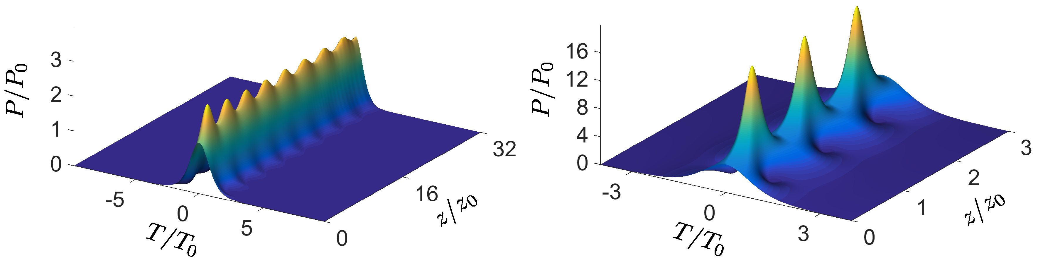
Figure 3.
Soliton and radiation energies as a function of soliton order N. Energy is normalized to units of fundamental soliton of Equation (5). The fundamental soliton is at the black dotted markers. Individual soliton energies (grey lines) add up to a cumulative value (piecewise linear blue trace); the latter approximates the total pulse energy (red dashed parabola). The difference between both is shown on an expanded, inverted scale in the lower part (green curve). From [2].

Figure 4.
Evolution of an Akhmediev breather at . .

Figure 5.
Evolution of a Peregrine soliton (left) and a Kuznetsov–Ma soliton (right). .

Figure 6.
Dispersion-managed fiber consists of alternatingly normally (dispersion compensating fiber (DCF)) and anomalously dispersive fiber (standard single mode fiber (SSMF)) segments. The dispersion parameter alternates between values of and ; the lengths of segments are and , respectively. The dispersion map period is .
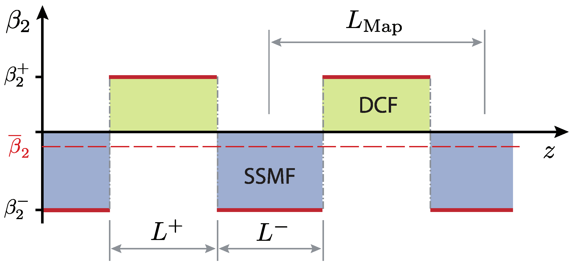
Figure 7.
Evolution of a dispersion-managed soliton over two dispersion map periods.

Figure 8.
Nonlinear spectrum calculated for a Gaussian pulse shape (Equation (18)) with and fulfilling Equation (4). (Left) The discrete spectrum, consisting of two solitons of the same center frequency. The reference energy here is chosen as . (Right) The power spectral density (PSD) of the linear radiation part.

Figure 9.
Direct scattering analysis of an soliton with different time window widths . The difference between the soliton energy found by direct scattering transform (DST) and the analytical value is shown. Labels on the right indicate the number of sample points used. Solid curve: expected truncation error, Equation (28) of the input pulse.
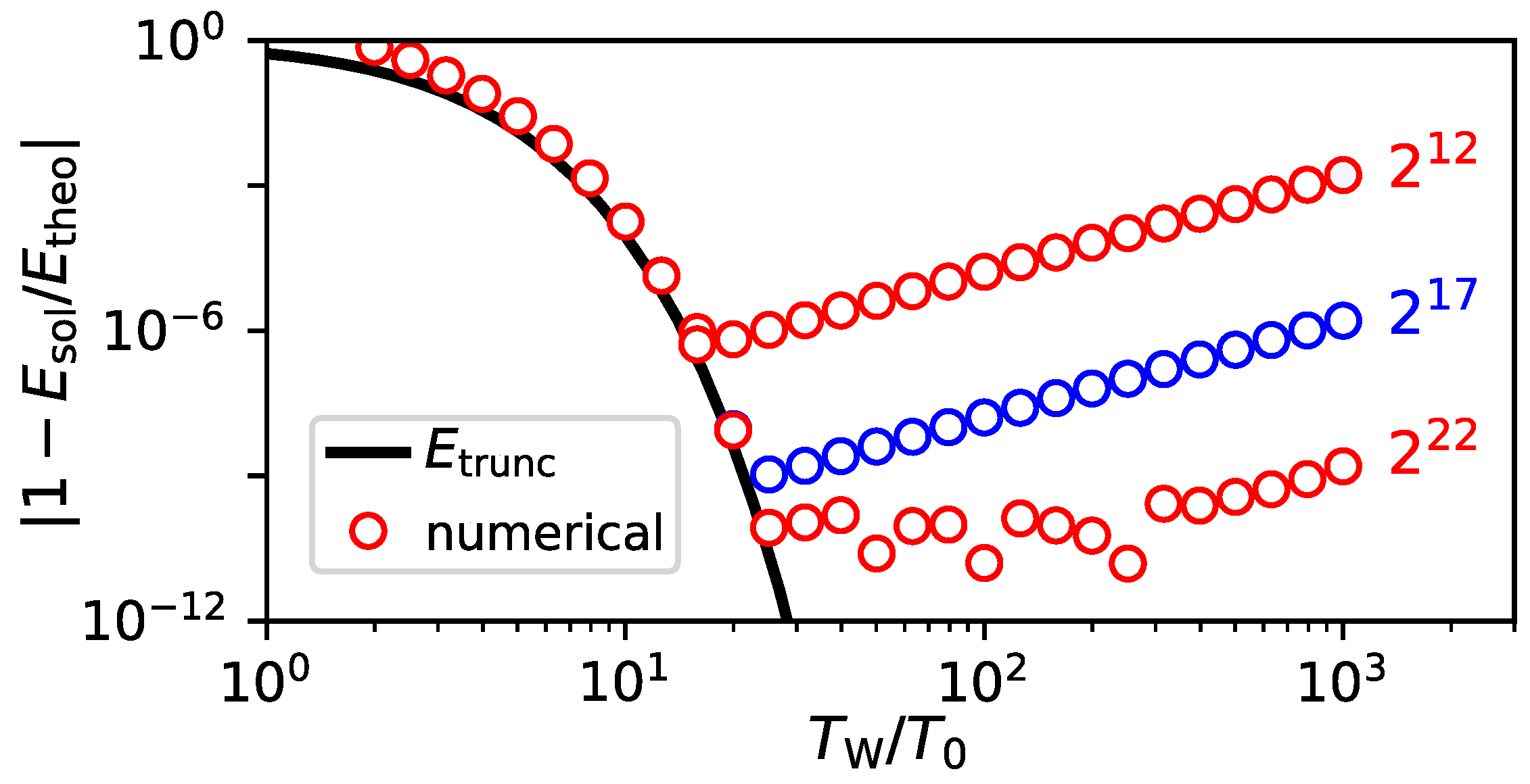
Figure 10.
Energy and frequency eigenvalues of a fundamental soliton obtained using the DST method. The soliton was perturbed by Raman self-frequency shift (blue, solid, Raman response time: ), third-order dispersion (orange, solid, TODparameter: ), and linear loss (green, dashed, loss length: ).
Figure 10.
Energy and frequency eigenvalues of a fundamental soliton obtained using the DST method. The soliton was perturbed by Raman self-frequency shift (blue, solid, Raman response time: ), third-order dispersion (orange, solid, TODparameter: ), and linear loss (green, dashed, loss length: ).
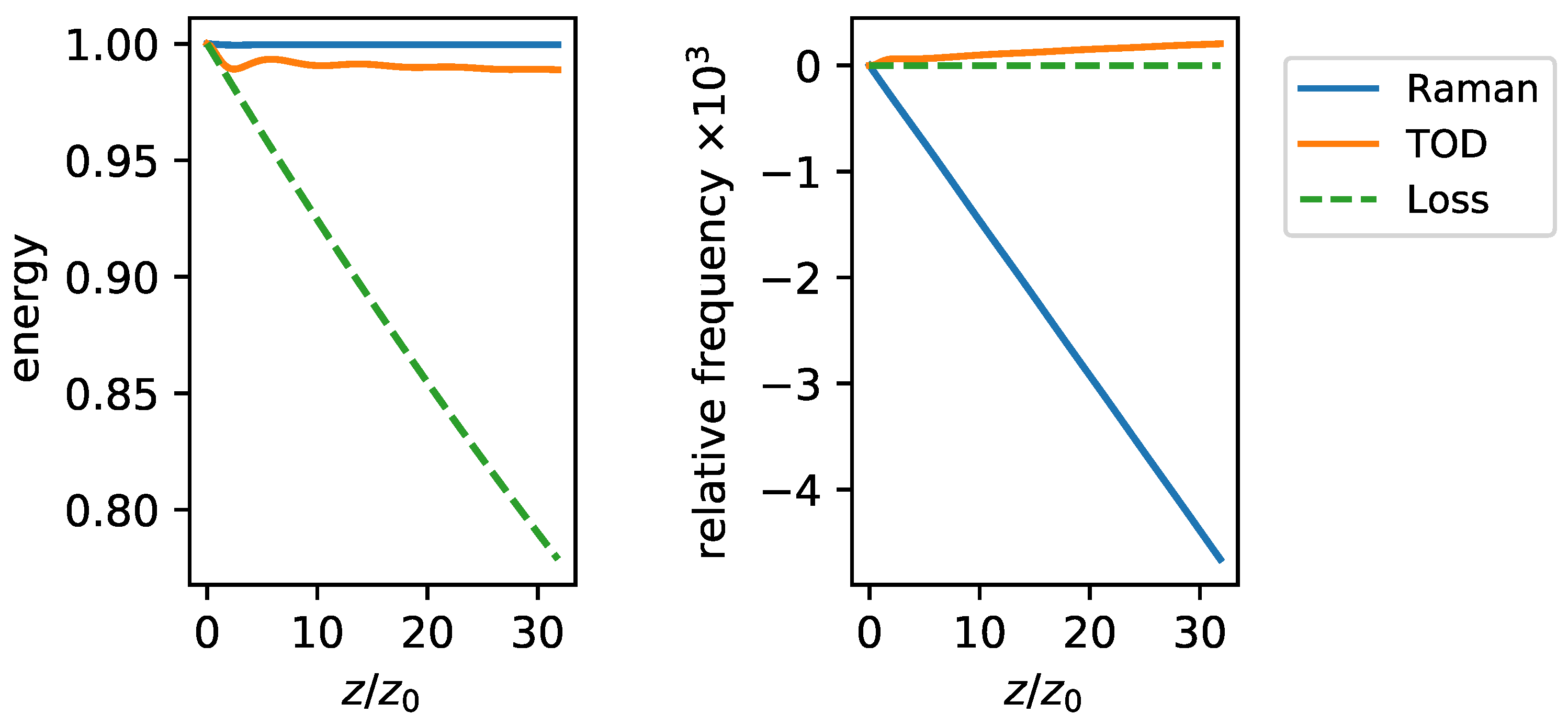
Figure 11.
(Left) Soliton radiation beat analysis (SRBA) chart from repeated numerical simulations with increasing soliton number N; (right) corresponding predictions of beat signals and its overtones (from [88]).
Figure 11.
(Left) Soliton radiation beat analysis (SRBA) chart from repeated numerical simulations with increasing soliton number N; (right) corresponding predictions of beat signals and its overtones (from [88]).
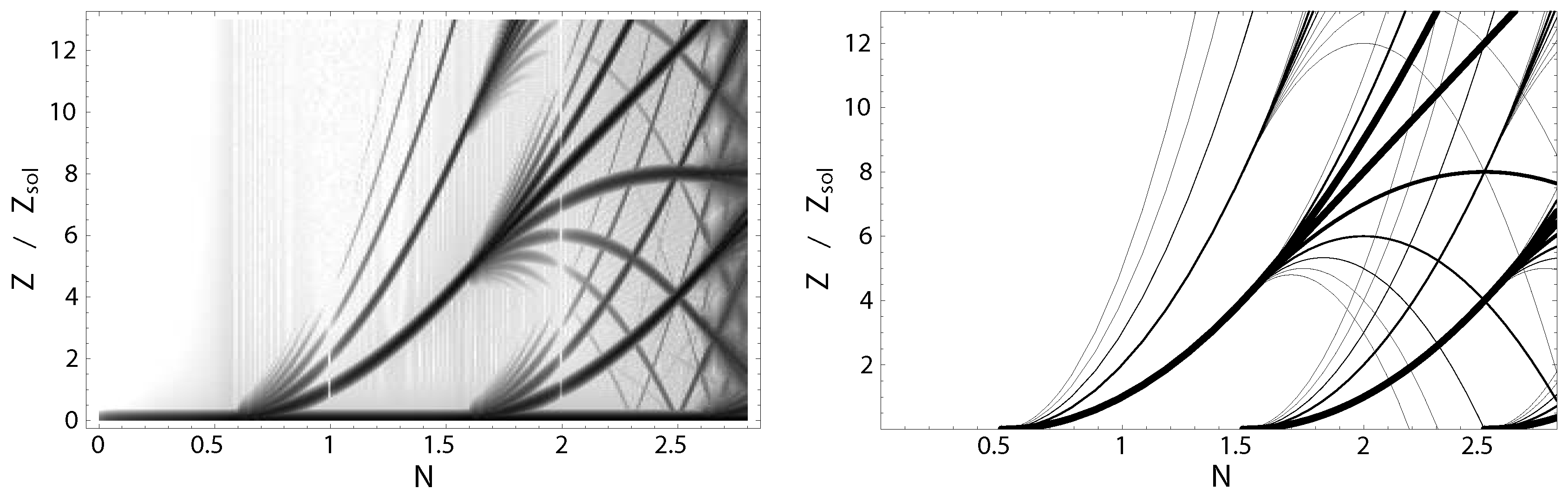
Figure 12.
Full-frequency SRBA chart to determine the soliton content of an soliton. Grey scale corresponds to the log of the Fourier transform of the spatial evolution of the spectral power density. Arrows labeled and mark traces pertaining to the first and second soliton; their beat note is also highlighted (from [93]).

Figure 13.
(Left) SRBA chart for an energy scan of a DM soliton. For an explanation of the procedure, and the apparent white vertical stripes in particular, see the text. (Right) Extract of the left panel, with standardized line types. The fundamentals pertaining to three constituent solitons are labeled –. The dashed line labeled ‘sol’ is for reference; it represents the spatial frequency for a non-DM soliton in a fiber with (from [93]).

© 2017 by the authors. Licensee MDPI, Basel, Switzerland. This article is an open access article distributed under the terms and conditions of the Creative Commons Attribution (CC BY) license (http://creativecommons.org/licenses/by/4.0/).
Share and Cite
MDPI and ACS Style
Mitschke, F.; Mahnke, C.; Hause, A. Soliton Content of Fiber-Optic Light Pulses. Appl. Sci. 2017, 7, 635. https://doi.org/10.3390/app7060635
AMA Style
Mitschke F, Mahnke C, Hause A. Soliton Content of Fiber-Optic Light Pulses. Applied Sciences. 2017; 7(6):635. https://doi.org/10.3390/app7060635
Chicago/Turabian StyleMitschke, Fedor, Christoph Mahnke, and Alexander Hause. 2017. "Soliton Content of Fiber-Optic Light Pulses" Applied Sciences 7, no. 6: 635. https://doi.org/10.3390/app7060635
Note that from the first issue of 2016, this journal uses article numbers instead of page numbers. See further details here.