
Remaining Useful Life Prediction of Hybrid Ceramic Bearings Using an Integrated Deep Learning and Particle Filter Approach


1
Department of Mechanical and Industrial Engineering, University of Illinois at Chicago, Chicago, IL 60607, USA
2
College of Mechanical Engineering and Automation, Northeastern University, Shenyang 110819, China
*
Author to whom correspondence should be addressed.
Appl. Sci. 2017, 7(7), 649; https://doi.org/10.3390/app7070649
Submission received: 31 March 2017
/
Revised: 7 June 2017
/
Accepted: 20 June 2017
/
Published: 23 June 2017
(This article belongs to the Special Issue Deep Learning Based Machine Fault Diagnosis and Prognosis)
Abstract
:Bearings are one of the most critical components in many industrial machines. Predicting remaining useful life (RUL) of bearings has been an important task for condition-based maintenance of industrial machines. One critical challenge for performing such tasks in the era of the Internet of Things and Industrial 4.0, is to automatically process massive amounts of data and accurately predict the RUL of bearings. This paper addresses the limitations of traditional data-driven prognostics, and presents a new method that integrates a deep belief network and a particle filter for RUL prediction of hybrid ceramic bearings. Real data collected from hybrid ceramic bearing run-to-failure tests were used to test and validate the integrated method. The performance of the integrated method was also compared with deep belief network and particle filter-based approaches. The validation and comparison results showed that RUL prediction performance using the integrated method was promising.
1. Introduction
Mechanical big data has the characteristics of large volume, diversity, and high velocity. The prediction of remaining useful life (RUL) has been used as an important parameter for condition-based maintenance decision making [1]. Traditional data-driven prognostic methods have their limitations for processing mechanical big data. Many prognostic methods are developed based on explicit model equations [2]. Therefore, they are largely dependent on human expertise and knowledge in model building and signal processing, and hence are difficult to implement for automatic processing of massive data. These prognostic methods include recurrent neural networks [3,4], Kalman filters [5,6,7], dynamic Bayesian networks [8], k-reliable decentralized prognosis [9], particle filter-based [10,11,12,13], and combined particle filter and neural networks [14]. In addition, some fuzzy systems-based approaches for prediction have been developed [15]. However, in comparison with fuzzy systems, particle filters take a probabilistic approach, in that the posterior distribution is modeled by sampling from a set of distributions, whereas in fuzzy systems the model output is based on the input variables of fuzzy set membership and an implication of rules. Among all the approaches, particle filters [16] have emerged in recent years as a comparatively good RUL prediction method and are becoming more and more widespread, mainly due to their capability of dealing with dynamic systems characterized with nonlinear and non-Gaussian natures. For example, Yoon and He [17] showed the superior RUL prediction performance of a particle filter-based approach using the gear data provided by the NASA Glenn Spiral Bevel Gear Test Facility.
However, all of the above mentioned methods require either complicated signal processing techniques to extract features from the sensor data, or knowledge of system dynamics to build the explicit model equations. This type of requirement involves manual processing and analysis of data by human experts, and therefore makes these methods unsuitable for automatic data processing and feature extraction for big data. There also may be situations in which these models are unavailable, such as in offshore well drilling and wind turbines, or for some bearings in which online measurements of the damage may not be available, in which the traditional particle filter approach cannot be used [11]. To effectively extract features from massive bearing condition monitoring data and accurately predict bearing RUL, new effective methods are needed. The recent developments in deep learning have provided an attractive opportunity to build advanced RUL prediction methods for big data.
Since the introduction of a deep belief network [18], deep belief networks and other deep learning methods have become widely used for big data processing and analysis. Deep learning is capable of extracting useful and important features from data to improve the power of prediction [19]. Equipped with multiple layers of structure, deep learning is also capable of processing massive data and extracting hidden information. One recent successful story of deep learning is AlphaGo by Google Deepmind [20]. AlphaGo has demonstrated the power of deep learning for massive data processing and feature learning by defeating the best human Go player in the world. Deep neural network architectures have been successfully built in various domains such as image recognition, automatic speech recognition, and natural language processing [21]. Recently [22,23] applied deep learning on raw vibration signals and time-domain features for machine fault diagnostics. In addition to classification problems, deep learning also has promising capability to solve prediction problems. These prediction problems include predicting car traffic [24], weather [25], wind speed [26], and internet traffic [27]. A number of deep learning algorithms have been used for solving prediction problems. These include auto-encoders, restricted Boltzmann machines, deep belief networks, convolutional neural networks, and more. Deep learning represents an attractive option to process massive data for RUL prediction. Deutsch and He [28] presented a deep learning-based bearing RUL prediction method using a deep brief network, and compared RUL prediction performance with a particle filter-based approach. Their comparison results showed that even though the RUL prediction performance of the deep learning based approach was comparable with particle filter-based approach, the RUL prediction accuracy of the deep learning-based approach was slightly lower than that of the particle filter. Therefore, it was of interest to investigate an integrated method that can use the strength of deep learning to overcome the limitations of the particle filter. To date, no research on combining deep learning with particle filter for RUL prediction of hybrid ceramic bearings has been reported in the literature.
In this paper, a new integrated method that combines a deep belief network with a particle filter for remaining useful life prediction of hybrid ceramic bearings using vibration signals was presented. Real vibration data collected from hybrid ceramic bearing run-to-failure tests were used to test and validate the integrated method. The performance of the integrated method was also compared with a deep belief network and particle filter-based approaches.
2. Methodology
A deep belief network (DBN), which is a stacked version of a restricted Boltzmann machine (RBM), and a purely data-driven particle filter were combined in this paper in order to predict the RUL at L steps ahead into the future. Next, the relevant background of RBM, DBN and the particle filter was provided. The section concludes with the combined DBN and particle filter-based approach for RUL prediction.
2.1. The Restricted Boltzmann Machine
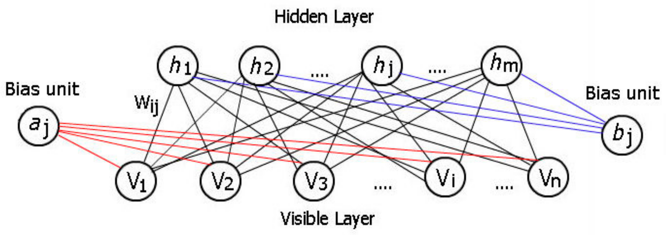
An RBM [29] is considered as a type of unsupervised machine learning method. It is a stochastic artificial neural network that learns a probability distribution over the set of its inputs. A RBM normally has two layers: a visible layer and a hidden layer. It can be represented by a bipartite graph that contains undirected edges from its two layers. Each layer contains a collection of neurons/nodes. Each neuron/node of the visible layer represents a feature of the input data, while neurons/nodes of the hidden layer represent the latent variables. A typical RBM structure is shown in Figure 1. The reason that an RBM is “Restricted” is because there are no connections between each neuron/node within either the visible or hidden layers. An RBM contains a matrix of weights representing the connection to visible node and hidden node . In Figure 1, represents the bias term in the visible layer, and in the hidden layer.
The weights and biases are computed by maximizing , the probability that the network assigns to a visible vector :
where is the normalization constant that can be obtained by summing over all the possible pairs of visible and hidden vectors:
and the energy function of the joint configuration is given by:
Theoretically, the problem of maximizing Equation (1) can be solved by taking its partial log derivative with respect to its parameters , and :
Normally Equation (4) can also be written as:
where < > denotes the expectation. However, the expectation in the maximum log likelihood function cannot be easily computed, and is thus estimated using contrastive divergence which leads to the following parameter updating equation [30]:
where represents a full step of Gibbs sampling, represents the learning rate and represents the of contrastive divergence. The neuron activation probabilities are given by the following equations:
where represents the number of visible units, the number of hidden units, and σ is the activation function. The activation function is typically the logistic function used as a threshold defined as:
2.2. The Deep Belief Network
A DBN is formed by stacking multiple RBMs on top of each other (see Figure 2) in order to create high representations of data that can be used for classification, regression (continuous output) tasks as well as unsupervised learning.
The RBM becomes a building block for forming a deep belief network. The DBN can be trained in a greedy-layer-wise fashion by stacking RBMs on top of each other [31]. The output of one RBM, that is the activation values in the hidden layer, simply becomes the input for the next RBM, and the parameters of the previous RBM do not change. This next RBM is trained by the same process as illustrated in the previous section. This process allows for creating multiple hidden layers.
In order to use a DBN to predict a continuous output, one can first learn the weights and biases in the unsupervised stage of learning. Once the optimal parameters (weights and biases) have been determined, a supervised fine tuning stage is performed. This is done by creating a final output layer on the top of the DBN which outputs the predicted RUL value, given a set of vibration features. This is illustrated in Figure 3. The parameters of the entire network are then updated using the back-propagation algorithm in the same way as a feedforward neural network (FNN) is trained. In this way, the DBN pre-trains the network, which serves as an initialization step for the parameters of the FNN, instead of a random initialization of the weights and biases, which has been shown to add robustness to deep architectures and decrease the probability of obtaining a poor local minima [32].
The DBN performs unsupervised learning first by training it on a set of signal features in order to learn a latent representation of the data. After the end of training, an output layer is added on top of the last layer of the DBN, where it is fully connected to the (last) hidden layer. This output layer contains one neuron (without an activation function) which represents the continuous prediction.
2.3. Particle Filter
The particle filter is a Monte Carlo approach that can be used to estimate the state of a system by combining both the state evolution of the system and the observation/measurement parameters obtained from the state.
In discrete time, a system can be described by the following state space model:
From the above equations, represents the state of the system (such as the crack depth) at time , which is independently and contains identically distributed (iid) noise/variance at time is a function that maps the transitions between states, represents the measurement/observation (can be thought of as a feature, typically derived from a vibration signal) at time , is the iid noise/variance associated with each measurement, and is a function that maps the state with the measurement.
The goal of the particle filter is then to be able to estimate the probability density function (pdf) of , that is, to estimate the state at time , given the measurements up to time It is also assumed that the prior probability of the state is unkown.
In the Bayesian setting, the state estimation is usually computed recursively in two stages; the prediction and the update. For the prediction step, the is given as:
For the update step, new measurements are collected, which are then used to update the prior distribution. The posterior distribution can then be written as:
Typically, the calculations for Equations (12) and (13) are intractable and the particle filter sampling approach is used to approximate them. This can be accomplished by using a set of samples/particles , where is the ith weight at time and is the user-specified number of particles generated. The weights can be updated by using the sequential importance resampling (SIR) algorithm [33], and samples are drawn from the state transition distribution:
Finally, the posterior distribution is obtained by resampling from where (predicted estimate) is drawn with probability .
2.4. Combined DBN and Particle Filter-Based Approaches for RUL Prediction
The ultimate objective of the combined DBN and particle filter approach is to estimate the pdf of , where and represents the length of the signal. It should be noted that no new (future) information about the system is provided at the generic time step , and only information provided from time steps may be used for the prediction.
There are two functions that are of interest in modeling; the state transition distribution Equation (14) (sometimes referred to as the proposal distribution) and the measurement distribution Equation (15). Both of these functions can be modeled by the DBN, since neural networks in general are universal function approximators [34].
In the prediction step, the state transition model can simply be approximated by first reconstructing the time series of the measurements ( for into a matrix, where each feature (column) represents a lagged order of the time series, and whose output is an L-step ahead into the future state value, and each row represents an index in time. Formally, the input can be denoted as:
and treat the state as the actual RUL of the bearing at time as the output:
where represents the embedding dimension, and determines the size of the first visible layer in the DBN. Thus, the network requires training tuples of the form , . Using this training set, the state transition model is instead actually modeling the pdf of . The step ahead prediction, is simply made by subtracting the network’s output by . The advantages of treating the state (instead of treating it as the crack depth for instance) as the actual RUL allow for a simpler model to be developed. One does not need to utilize another neural network to determine the RUL, given the crack depth, or to recursively compute the state transition model multiple times until it exceeds such a threshold, which needs to be defined. By training the network directly on the RUL, the network is minimizing the error of predicting the RUL, rather than an intermediate value. This results in a network that is more easily trainable and reduces the potential problem of having the network’s eventual forecast of the state die off (converging to a single value). The disadvantage of this approach however, is that the parameters of the state transition model will be updated/relearned less frequently. The measurement (often a multi dimensional vector) can be constructed into a mono-dimensional feature vector by setting the input of the DBN as and then setting the size of the last hidden layer to one. The output of the DBN in its unsupervised stage of learning is then the reconstructed mono-dimensional feature vector of .
Equations (16) and (17) define a method often called the sliding window technique [35]. This windowing approach is illustrated in Figure 4.
The first plot in Figure 4 is the complete series of a fault feature. The second plot highlights the first window of size = 100. The last figure simply shows a zoom-in of the first window. The first window contains points from (first row of features), and the second window would contain points from (second row of features), and so on.
The state transition model and its respective variance in Equation (10) can be modeled by taking bootstraps, which randomly samples (with replacement) each row of the training data times. The DBN is then trained times for each bootstrap and the predicted values will be defined as:
where, represents the generic testing input vector of the past measurements [Equation (16)] and represents the DBN-FNN output [Equation (17)] with respect to the bootstrap. The mean and variance are simply then calculated as:
and then samples can be generated from the following Gaussian distribution:
The measurement distribution can be modeled in a somewhat similar approach to the state transition distribution. The technique [13] requires a dataset of tuples of where bootstraps are sampled from this training data set, and an interpolator is created. is typically a multi-dimensional vector, which can be reduced to a single mono-dimensional vector for simplicity and ease of calculation. This can be performed by the DBN in its unsupervised stage of learning, by setting the last layer of the DBN’s hidden layer to a size of one. A simple FFN can also be used as an interpolator for computing the following:
where, is the th bootstrap sampled from the dataset. The measurement model in Equation (11) can be hypothesized as:
From Equation (23), we can subtract from both sides such that:
The error term is then a function of and , which we will call the model error and intrinsic noise respectively. Their variances are then denoted as and respectively. The model error variance can be modeled by taking groups of interpolators from of length networks and computing the average as:
The set, is then resampled with replacement using bootstraps, denoted as , where is the th bootstrap of . The estimate of the model error variance can then be computed as:
The noise variance can be modeled by building up a training set , where is defined as:
A single FNN can then be trained on the aforementioned training set in order to estimate for an arbitrary vector. Finally can be approximated by:
The confidence intervals for a generic prediction can then be obtained with 1-% confidence by the following formula [36]:
The training/testing procedure for the integrated DBN and particle filter is then as follows:
| Step 1 | Let the last 100 rows be equal to the testing set, and set the rest of the data to the training set. | |
| Step 2 | Approximate the state transition model. | |
| a | Reconstruct the time series of the signal features into a matrix with an embedding dimension of . This will serve as the input, and the output will be the mapped state , where . | |
| b | Create bootstrapped data sets using the data created in Step 1. | |
| c | Initialize the weights and biases of the FNN by training the DBN on the input data with all the data except for the last 100 rows. The rest of the data is the testing set. | |
| d | Train the FNN. Fine tune the weights in a supervised fashion by minimizing the loss function on the training set and by using the back-propagation algorithm. | |
| e | Predict the . This is accomplished by subtracting the network’s output by L, i.e., = . | |
| f | Let , and update the training vector with input features . | |
| g | Repeat Steps 2e–2f, until all 100 points have been predicted. | |
| Step 3 | Estimate the measurement distribution. Create a new dataset of the form Generate B bootstraps from this training dataset and apply Equations (22)–(28) to obtain the measurement distribution. The DBN can be used for estimates in Equations (22) and (27). | |
| Step 4 | Estimate the state. The predicted state can be obtained by sampling with probability [from Equation (15)]. | |
This method allows a complete data-driven approach to be developed in conjunction with a particle filter for RUL estimation. Equation (10), the proposal distribution is built up using training tuples of the form . The bootstrapping approach is then used to collect the statistics for the mean and variance. Equation (11), the measurement model is then modeled by Equations (22)–(28). Here the DBN can serve two purposes. It can be used to reduce the dimensionality of the measurement and it can also to be used in order to initialize the weights of the neural network.
3. Validation
In this section, the validation of the integrated bearing RUL prediction method using vibration data collected from a single hybrid ceramic bearing run-to-failure test is discussed.
3.1. Hybrid Ceramic Bearing Run-to-Failure Test Setup
The hybrid ceramic bearing run-to-failure tests were performed using a bearing test rig in the laboratory as shown in Figure 5. The bearing test rig consisted of the following main components: (1) 3-HP AC motor with a maximum speed up to 3600 rpm and variable speed controller; (2) Hydraulic dynamic loading system with a maximum radial load up to 4400 lbs or 19.64 kN; (3) Integrated loading and bearing housing. The rig can be used for testing both ball and tapered roller bearings.
An automatic data acquisition system was constructed using a National Instrument CI 4462 board (NI, Austin, TX, USA) and NI LabVIEW software (LabView 2012, NI, Austin, TX, USA). The automatic data acquisition system is characterized with the following key features: (1) Maximum sampling rate up to 102.4 kHz; (2) 4 Input simultaneous anti-aliasing filters; (3) Software-configurable AC/DC coupling and IEPE conditioning; (4) Vibration analysis functions such as envelope analysis, cepstrum analysis, and so on for computing necessary condition indicators.
The tested hybrid ceramic ball bearing was a SMR6205C-ZZ/C3 #3 L55/MG2 type bearing by Boca Bearing Company (Boca Bearings, Boynton Beach, FL, USA). It consisted of stainless steel inner outer races, and ceramic balls. The bearing was mounted on the test rig. Two accelerometers were stunt mounted on the bearing housing in the direction perpendicular to the shaft. During the tests, the rig was run at a speed of 1800 rpm (30 Hz) and was subjected to a radial load of 600 psi. Vibration data were collected with a sampling rate of 102.4 kHz for two seconds at each sampling point. There was a 5 min gap between any two sampling points. At the end of the test, the test bearing was disassembled, checked, and photographed. The bearing data contained a total of 849 data files with a length of approximately 71 hours. Table 1 describes the run-to-failure test setting. Table 2 provides the specifications of the tested bearing.
The root mean square (RMS) of the vibration signals was computed to represent the degradation of the bearing over time during the run to failure tests. The RMS at each time interval (denoted as ) can be calculated as follows:
where represents the raw vibration data point at time interval and is the length of the signal at time interval . The RMS for the bearing data can be seen in Figure 6.
For the bearing data, the (remaining useful life at time ) was calculated simply by taking the time index of the maximum recorded RMS value as the point of failure denoted as and subtracting it from each time step:
The raw vibration signals were preprocessed using the fast Fourier transform (FFT), and the FFT values were used as the only signal feature input into the integrated DBN-particle filter model to predict the RUL of the bearing. The FFT, which is an efficient algorithm for computing the discrete Fourier transform (DFT) at a time interval , can be calculated as follows:
where is the raw vibration signal at time interval , is the length of the signal at time interval , , and = 0,1,…,.
Equation (31) transforms the vibration signals from a time domain to a frequency domain in which we extracted ten equal bands ranging from 0 to 20 kHz.
3.2. Hybrid Ceramic Bearing RUL Prediction Results
A total of 849 time steps were extracted from the bearing data in which all the data up until time step 792 were used. As seen from Figure 6, a rather large dip in the RMS values occurred from time steps 720 through 735. Features collected from those points were simply removed from the data and treated as outliers.
= 1 and were used to predict 5 min and 50 min into the future for the bearing data, respectively.
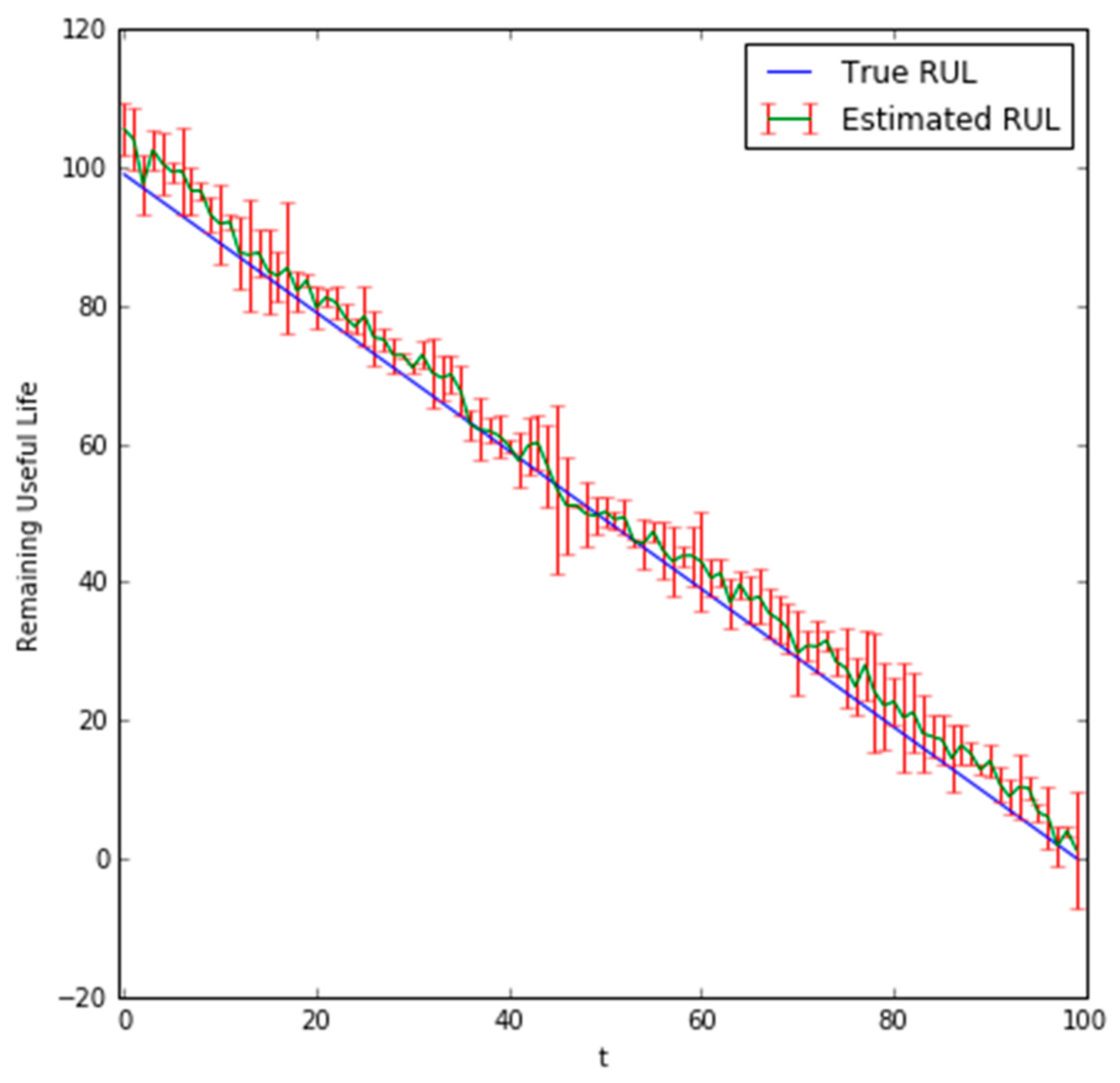
The predicted RUL values for the last 100 steps can be seen in Figure 7 and Figure 8 for = 1 and = 10, respectively. The error metrics and hyperparameters of the DBN with = 1 and = 10 are provided in Table 3 and Table 4, respectively. Table 4 shows the hyperparameters of the DBN for the state transition model which were determined using a grid search. Input data was also scaled to be in [0, 1], = 100 was set as the embedding dimension, was set as 50, and 50 particles were used for both = 1 and = 10 predictions.
In Figure 7 and Figure 8, the green color represents the average predicted RUL values across the bootstrapped samples. The red error bars represent the 95% bounds. The predicted results show for both = 1 and = 10 that it can accurately predict the true RUL, and as the bearing approaches the point of failure, the accuracy of the predictions tends to increase.
The confidence bounds for the = 10 predicts the RUL of the bearing slightly early when compared to the = 1 predictions and exhibits a greater variance.
The common error metrics used in Table 3 are the root mean squared error (RMSE), metric [37,38], and the mean absolute percentage error (MAPE). The MAPE, RMSE, and metric are defined by the following equations:
In Equations (33) and (34), denotes the actual value, represents the predicted value, and equals the number of points to be predicted. In Equation (35), represents a user specified bound level, represents the actual RUL at time , and represents the predicted RUL at time . is given as a percentage of RUL for a given equipment (i.e., represents the time index where half the RUL is left). The reported in Table 3 represents the average metric across the all testing samples. In the metric, results closer to one indicate better performance. The loss functions used to train the state transition models for and were the MSE () and the MAPE respectively. Satisfactory hyperparameters for building up Equations (22) and (27) for both and were set as [105, 59] for the hidden layer structure using 122 epochs with a learning rate of 0.00085. The hyperparameters for the reconstructed mono-dimensional measurement data were set as [142, 87] for the hidden layer structure using a small learning rate of 0.0094 and 212 epochs. The hyperparameters for each built network was done by employing a grid search and evaluating candidate hyperparameters on the MSE using a 10 fold cross validation on the training set. Cross validation is a widely used method to avoid overftting when selecting hyperparameters [39]. The chosen hyperparameters were obtained by those that minimized the MSE during cross validation. For all of these networks, the activation function was set as the rectified linear unit (ReLU) function. It solves the vanishing gradient problem that other non-linear activation functions can cause [40]. The ReLU activation function for the input of a neuron is defined as:
Since the particle filter is the most competitive RUL prediction method for bearings, for a comparison purpose, the RMSE and MAPE of the RUL predictions obtained by the particle filter-based approach are also provided in Table 3. In comparison with the results obtained using the particle filter-based approach, the RMSE and MAPE values of the integrated approach were slightly lower and the metric values were higher. Note that since in [28], it was reported that using the same bearing data, the particle filter gave a better RUL prediction accuracy than a DBN based approach did, we consider the integrated method presented here as better than the DBN-based approach used on the same dataset. The comparison results showed the promising performance of combining the deep learning based approach with particle filter for hybrid ceramic bearing RUL prediction.
Given that the integrated approach did not require explicit model equations like the particle filter-based approach and is scalable for big data applications, the RUL prediction performance achieved by the integrated approach has shown great potential for bearing RUL prediction with big data.
4. Conclusions
Predicting the remaining useful life of bearings has been an important task for condition-based maintenance of industrial machines, as bearings are one of the most critical components in these machines. To meet the challenge of automatically processing massive data and accurately predicting RUL of the bearings in the era of the Internet of Things and Industrial 4.0, this paper addressed the limitations of traditional data-driven prognostics by presenting a new method that integrates a deep belief network and a particle filter for RUL prediction of hybrid ceramic bearings. Real vibration data collected from hybrid ceramic bearing run-to-failure tests were used to test and validate the integrated method. The performance of the integrated method was also compared with DBN and particle filter-based approaches. In comparison with the RUL prediction results obtained using the particle filter-based method, the prediction accuracy measured by RMSE and MAPE of the integrated method is slightly lower. Also, based on the previous comparison between DBN and the particle filter methods for the same dataset reported in [28], the RUL prediction performance of the integrated method is considered better than the DBN method. The validation and comparison results showed the promising RUL prediction performance of the integrated method.
Since the integrated approach was a purely data-driven approach, future work should focus on increasing user confidence in the method. This may be accomplished by combining the integrated approach with other techniques such as employing the use of fuzzy similarity [41]. This would require a large database of run to fail trajectories that can be compared based on their similarity with the observed data. This large database should not only increase the accuracy of the integrated approach, but also further validate it. Additional work may also include the processing of the raw vibration signals at each sampling interval by a DBN into a single dimension signal feature that can be used for prognostics.
Author Contributions
Jason Deutsch conceived the idea and formulated the mathematical models behind the provided approach. In addition, he was responsible for all parameter tuning, data processing, figures, and calculations. Miao He was responsible for the run to fail trajectories of the hybrid ceramic bearings in the experimental setup. David He was responsible for research idea generation, the introduction, abstract, conclusions, and for the final editing and reviewing of the provided approach.
Conflicts of Interest
The authors declare no conflict of interest.
References
- Huynh, K.T.; Castro, I.T.; Barros, A.; Bérenguer, C. On the use of mean residual life as a condition index for condition-based maintenance decision-making. IEEE Trans. Syst. Man Cybern. Syst. 2014, 44, 877–893. [Google Scholar] [CrossRef]
- Vachtsevanos, G.; Lewis, F.L.; Roemer, M.; Hess, A.; Wu, B. Intelligent Fault Diagnosis and Prognosis for Engineering System; John Wiley & Sons, Inc.: Hoboken, NJ, USA, 2006. [Google Scholar]
- Malhi, A.; Yan, R.; Gao, R.X. Prognosis of defect propagation based on recurrent neural networks. IEEE Trans. Instrum. Meas. 2011, 60, 703–711. [Google Scholar] [CrossRef]
- Heimes, F. Recurrent neural networks for remaining useful life estimation. In Proceedings of the 2008 IEEE International Conference of Prognostics and Health Management, Denver, CO, USA, 6–9 October 2008; pp. 1–6. [Google Scholar]
- Lim, P.; Goh, C.K.; Tan, K.C.; Dutta, P. Estimation of remaining useful life based on switching Kalman filter neural network ensemble. In Proceedings of the 2014 Annual Conference of the Prognostics and Health Management Society, Fort Worth, TX, USA, 29 September–2 October 2014; pp. 2–9. [Google Scholar]
- Baraldi, P.; Mangili, F.; Zio, E. A Kalman filter-based ensemble approach with application to turbine creep prognostics. IEEE Trans. Reliab. 2012, 61, 966–977. [Google Scholar] [CrossRef]
- Bechhoefer, E.; Clark, S.; He, D. A state space model for vibration based prognostics. In Proceedings of the 2010 Annual Conference of the Prognostics and Health Management Society, Portland, OR, USA, 10–16 October 2010. [Google Scholar]
- Codetta-Raiteri, D.; Portinale, L. Dynamic Bayesian networks for fault detection, identification, and recovery in autonomous spacecraft. IEEE Trans. Syst. Man Cybern. Syst. 2015, 45, 13–24. [Google Scholar] [CrossRef]
- Yin, X.; Li, Z. Reliable decentralized fault prognosis of discrete-event systems. IEEE Trans. Syst. Man Cybern. Syst. 2016, 46, 1598–1603. [Google Scholar] [CrossRef]
- Daigle, M.J.; Goebel, K. Model-based prognostics with concurrent damage progression processes. IEEE Trans. Syst. Man Cybern. Syst. 2013, 43, 535–546. [Google Scholar] [CrossRef]
- Baraldi, P.; Compare, M.; Sauco, S.; Zio, E. Ensemble neural network-based particle filtering for prognostics. Mech. Syst. Signal Process. 2013, 41, 288–300. [Google Scholar] [CrossRef]
- Chen, C.; Zhang, B.; Vachtsevanos, G.; Orchard, M. Machine condition prediction based on adaptive neuro–fuzzy and high-order particle filtering. IEEE Trans. Ind. Electron. 2011, 58, 4353–4364. [Google Scholar] [CrossRef]
- He, D.; Bechhoefer, E.; Ma, J.; Li, R. Particle filtering based gear prognostics using one-dimensional health index. In Proceedings of the 2011 Annual Conference of the Prognostics and Health Management Society, Montreal, QC, Canada, 25–29 September 2011. [Google Scholar]
- Daroogheh, N.; Baniamerian, A.; Meskin, N.; Khorasani, K. Prognosis and health monitoring of nonlinear systems using a hybrid scheme through integration of PFs and neural networks. IEEE Trans. Syst. Man Cybern. Syst. 2016, PP, 1–15. [Google Scholar] [CrossRef]
- Bououden, S.; Chadli, M.; Allouani, F.; Filali, S. A new approach for fuzzy predictive adaptive controller design using particle swarm optimization algorithm. Int. J. Innov. Comput. Inf. Control 2013, 9, 3741–3758. [Google Scholar]
- Arulampalam, M.S.; Makell, S.; Gordon, N.; Clapp, T. A tutorial on particle filters for online nonlinear/non-Gaussian Bayesian tracking. IEEE Trans. Signal Process. 2002, 50, 174–188. [Google Scholar] [CrossRef]
- Yoon, J.; He, D. Development of an efficient prognostic estimator. J. Fail. Anal. Prev. 2015, 15, 129–138. [Google Scholar] [CrossRef]
- Hinton, G.E.; Osindero, S.; Teh, Y.-W. A fast learning algorithm for deep belief nets. Neural Comput. 2006, 18, 1527–1554. [Google Scholar] [CrossRef] [PubMed]
- Bengio, Y.; Courville, A.; Vincent, P. Representation learning: A review and new perspectives. IEEE Trans. Pattern Anal. Mach. Intell. 2013, 35, 1798–1828. [Google Scholar] [CrossRef] [PubMed]
- Silver, D.; Huang, A.; Maddison, C.J.; Guez, A.; Sifre, L.; Van Den Driessche, G.; Schrittwieser, J.; Antonoglou, I.; Panneershelvam, V.; Lanctot, M.; et al. Mastering the game of Go with deep neural networks and tree search. Nature 2016, 529, 484–489. [Google Scholar] [CrossRef] [PubMed]
- LeCun, Y.; Bengio, Y.; Hinton, G. Deep learning. Nature 2015, 521, 436–444. [Google Scholar] [CrossRef] [PubMed]
- Chen, Z.; Zeng, X.; Li, W.; Liao, G. Machine fault classification using deep belief network. In Proceedings of the 2016 IEEE International Instrumentation and Measurement Technology Conference, Taipei, Taiwan, 23–26 May 2016; pp. 1–6. [Google Scholar]
- Shao, H.; Jiang, H.; Zhang, X.; Niu, M. Rolling bearing fault diagnosis using an optimization deep belief network. Meas. Sci. Technol. 2015, 26, 115002. [Google Scholar] [CrossRef]
- Lv, Y.; Duan, Y.; Kang, W.; Li, Z.; Wang, F.-Y. Traffic flow prediction with big data: A deep learning approach. IEEE Trans. Intell. Transp. Syst. 2015, 16, 865–873. [Google Scholar] [CrossRef]
- Hossain, M.; Rekabdar, B.; Louis, S.J.; Dascalu, S. Forecasting the weather of Nevada: A deep learning approach. In Proceedings of the 2015 International Joint Conference on Neural Networks (IJCNN), Killarney, Ireland, 12–17 July 2015; pp. 1–6. [Google Scholar]
- Tao, Y.; Chen, H.; Qiu, C. Wind power prediction and pattern feature based on deep learning method. In Proceedings of the 2014 IEEE PES Asia-Pacific Power and Energy Engineering Conference (APPEEC), Hong Kong, China, 7–10 December 2014; pp. 1–4. [Google Scholar]
- Oliveira, T.P.; Barbar, J.S.; Soares, A.S. Multilayer perceptron and stacked autoencoder for Internet traffic prediction. In Proceedings of the 11th IFIP International Conference on Network and Parallel Computing (NPC), Ilan, Taiwan, 18–20 September 2014; Springer: Berlin/Heidelberg, Germany, 2014; pp. 61–71. [Google Scholar]
- Deutsch, J.; He, D. Using deep learning based approach to predict remaining useful life of rotating components. IEEE Trans. Syst. Man Cybern. Syst. 2017, PP, 1–10. [Google Scholar] [CrossRef]
- Smolensky, P. Information Processing in Dynamical Systems: Foundations of Harmony Theory. In Parallel Distributed Processing: Explorations in the Microstructure of Cognition, Volume 1: Foundations; MIT Press: Cambridge, MA, USA, 1986; Chapter 6; pp. 194–281. [Google Scholar]
- Hinton, G.E. Training products of experts by minimizing contrastive divergence. Neural Comput. 2002, 14, 1711–1800. [Google Scholar] [CrossRef] [PubMed]
- Bengio, Y.; Lamblin, P.; Popovici, D.; Larochelle, H. Greedy layer-wise training of deep networks. In Proceedings of the 19th International Conference on Neural Information Processing Systems, Vancouver, BC, Canada, 4–7 December 2006; MIT Press: Cambridge, MA, USA, 2006; Volume 19, pp. 153–160. [Google Scholar]
- Erhan, D.; Bengio, Y.; Courville, A.; Manzagol, P.; Vincent, P.; Bengio, S. Why does unsupervised pre-training help deep learning? J. Mach. Learn. Res. 2010, 11, 625–660. [Google Scholar]
- Gordon, N.; Salmond, D.; Smith, A. Novel approach to nonlinear/non-Gaussian Bayesian state estimation. IEE Proc. F Radar Signal Process. 1993, 140, 107–113. [Google Scholar] [CrossRef]
- Hornik, K.; Stinchcombe, M.; White, H. Multilayer feedforward networks are universal approximators. Neural Netw. 1989, 2, 359–366. [Google Scholar] [CrossRef]
- Frank, R.J.; Davey, N.; Hunt, S.P. Time series prediction and neural networks. J. Intell. Robot. Syst. 2001, 31, 91–103. [Google Scholar] [CrossRef]
- Khosravi, A.; Nahavandi, S.; Creighton, D.; Atiya, A.F. Comprehensive review of neural network-based prediction intervals and new advances. IEEE Trans. Neural Netw. 2011, 22, 1341–1356. [Google Scholar] [CrossRef] [PubMed]
- Al-Dahidi, S.; Di Maio, F.; Baraldi, P.; Zio, E. Remaining useful life estimation in heterogeneous fleets working under variable operating conditions. Reliab. Eng. Syst. Saf. 2016, 156, 109–124. [Google Scholar] [CrossRef]
- Saxena, A.; Celaya, J.; Saha, B.; Saha, S.; Goebel, K. Metrics for offline evaluation of prognostic performance. Int. J. Progn. Health Manag. 2010, 1, 4–23. [Google Scholar]
- Bergstra, J.; Bengio, Y. Random search for hyper-parameter optimization. J. Mach. Learn. Res. 2002, 13, 281–305. [Google Scholar]
- Glorot, X.; Bordes, A.; Bengio, Y. Deep sparse rectifier neural networks. In Proceedings of the Fourteenth International Conference on Artificial Intelligence and Statistics (AISTATS), Ft. Lauderdale, FL, USA, 11–13 April 2011; pp. 315–323. [Google Scholar]
- Maio, F.; Zio, E. Failure prognostics by a data-driven similarity-based approach. Int. J. Reliab. Qual. Saf. Eng. 2013, 20, 1–17. [Google Scholar]
Figure 1.
A restricted Boltzmann machine.

Figure 2.
A deep belief network with two hidden layers.
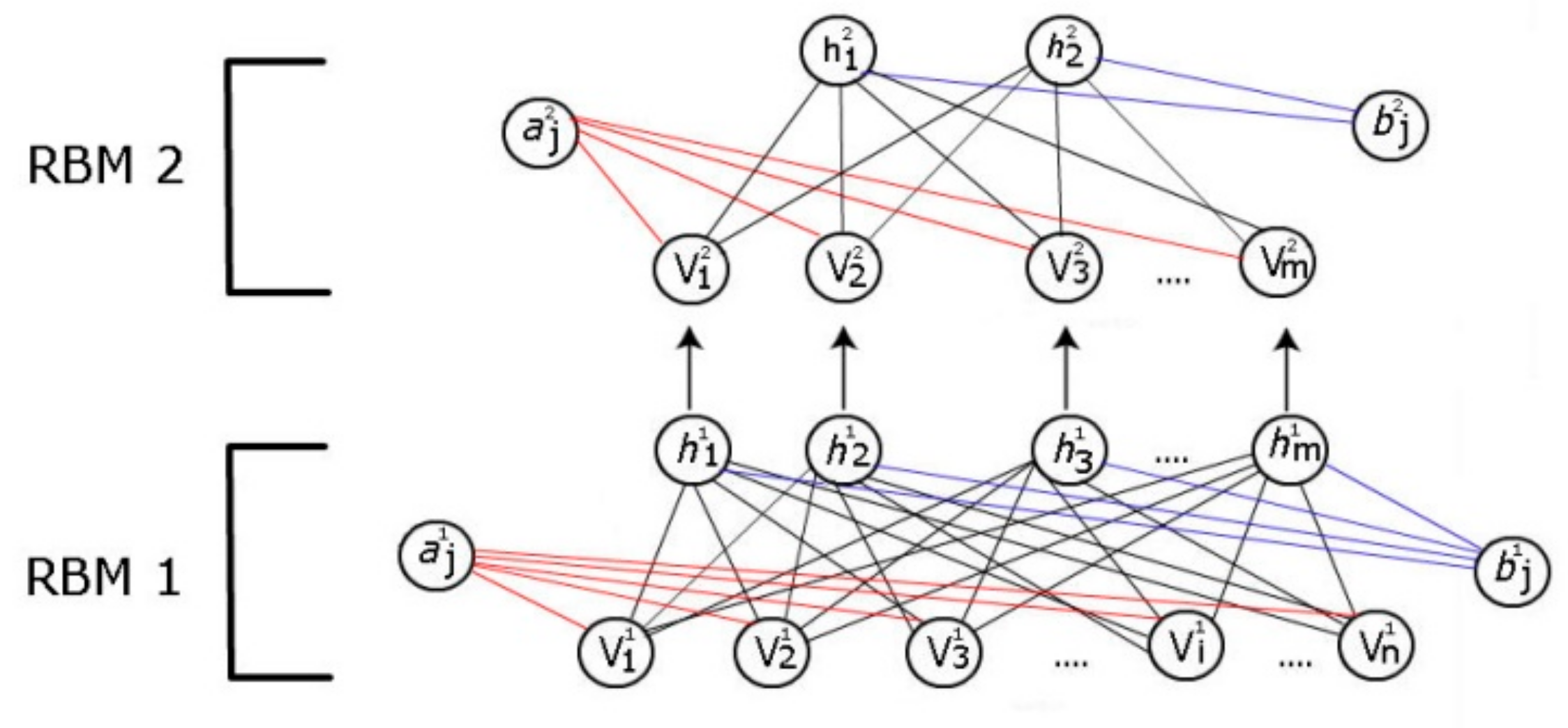
Figure 3.
A feedforward neural network with and a single hidden layer.
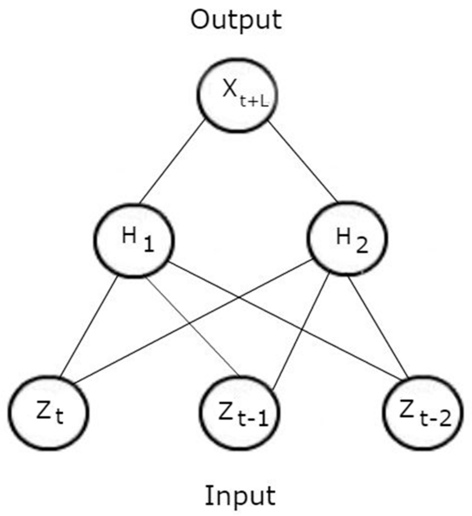
Figure 4.
The windowing approach.
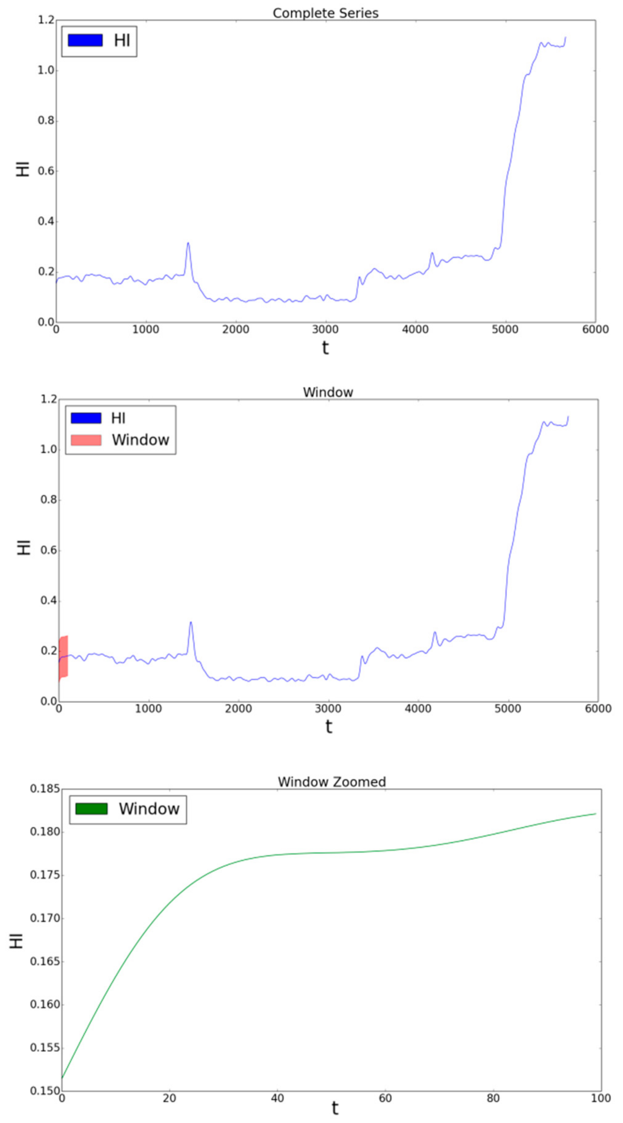
Figure 5.
The bearing run-to-failure test rig.

Figure 6.
The bearing RMS values.
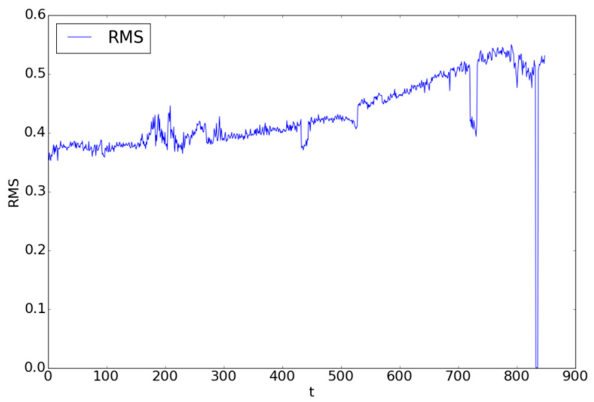
Figure 7.
Plot of bearing values with = 1.
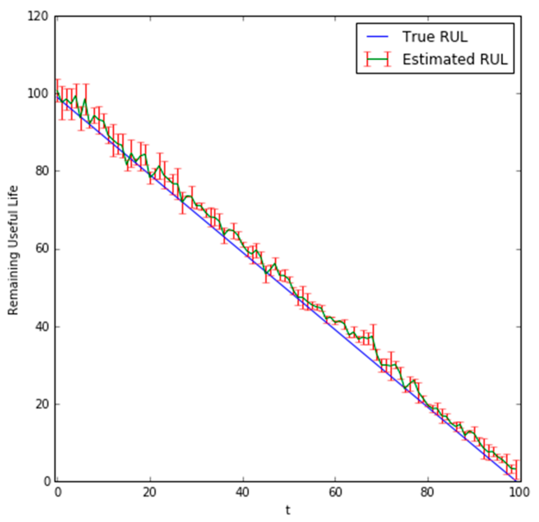
Figure 8.
Plot of bearing values with = 10.


Table 1.
The settings of the run-to-failure test.
| Test Bearing Name | Type of Bearing | Load (psi) | Input Shaft Speed (hz) |
|---|---|---|---|
| B2 | Hybrid ceramic bearing | 600 | 30 |
Table 2.
Specifications of the test bearing.
| Parameter | Specification |
|---|---|
| Bearing material | Stainless steel 440c |
| Ball material | Ceramic SI3N4 |
| Inner diameter (d) | 25 mm |
| Outer diameter (D) | 52 mm |
| Width | 15 mm |
| Enclosure | Two shields |
| Enclosure material | Stainless steel |
| Enclosure type | Removable (S) |
| Retainer material | Stainless steel |
| ABEC/ISO rating | ABEC #3/ISOP6 |
| Radial play | C3 |
| Lube | Klubber L55 grease |
| RPM grease (×1000 rpm) | 19 |
| RPM oil (×1000): | 22 |
| Dynamic load (kgf) | 1429 |
| Basic load (kgf) | 804 |
| Working temperature (°C) | 121 |
| Weight (g) | 110.32 |
Table 3.
Root mean squared error (RMSE) and mean absolute percentage error (MAPE) results.
| Combined DBN and Particle Filter-Based Approach | |||
|---|---|---|---|
| RMSE | MAPE | Accuracy (α = 10%) | |
| 1 | 2.04 | 7.33% | 0.80 |
| 10 | 3.52 | 8.68% | 0.61 |
| Particle Filter-Based Approach | |||
| RMSE | MAPE | Accuracy (α = 10%) | |
| 1 | 2.53 | 7.47% | 0.71 |
| 10 | 3.65 | 8.73% | 0.53 |
Table 4.
Hyperparameters of the deep belief network (DBN).
| DBN Learning Rate | DBN Epochs | Hidden Layer Structure | FNN Learning Rate | FNN Epochs | |
|---|---|---|---|---|---|
| 1 | 0.002 | 74 | [146, 53] | 0.0017 | 176 |
| 10 | 0.0023 | 82 | [120, 54] | 0.0014 | 92 |
© 2017 by the authors. Licensee MDPI, Basel, Switzerland. This article is an open access article distributed under the terms and conditions of the Creative Commons Attribution (CC BY) license (http://creativecommons.org/licenses/by/4.0/).
Share and Cite
MDPI and ACS Style
Deutsch, J.; He, M.; He, D. Remaining Useful Life Prediction of Hybrid Ceramic Bearings Using an Integrated Deep Learning and Particle Filter Approach. Appl. Sci. 2017, 7, 649. https://doi.org/10.3390/app7070649
AMA Style
Deutsch J, He M, He D. Remaining Useful Life Prediction of Hybrid Ceramic Bearings Using an Integrated Deep Learning and Particle Filter Approach. Applied Sciences. 2017; 7(7):649. https://doi.org/10.3390/app7070649
Chicago/Turabian StyleDeutsch, Jason, Miao He, and David He. 2017. "Remaining Useful Life Prediction of Hybrid Ceramic Bearings Using an Integrated Deep Learning and Particle Filter Approach" Applied Sciences 7, no. 7: 649. https://doi.org/10.3390/app7070649
Note that from the first issue of 2016, this journal uses article numbers instead of page numbers. See further details here.