Modified Godard Timing Recovery for Non Integer Oversampling Receivers
by

Arne Josten
*, 
Benedikt Baeuerle
,
Edwin Dornbierer
,
Jonathan Boesser
,
David Hillerkuss
and
Juerg Leuthold
ETH Zurich, Institute of Electromagnetic Fields (IEF), Zurich 8092, Switzerland
*
Author to whom correspondence should be addressed.
Appl. Sci. 2017, 7(7), 655; https://doi.org/10.3390/app7070655
Submission received: 19 May 2017
/
Revised: 18 June 2017
/
Accepted: 21 June 2017
/
Published: 24 June 2017
(This article belongs to the Special Issue Optical Signal Processing: Advances and Perspectives)
Abstract
:A timing recovery algorithm is introduced that operates with less than two samples per symbol and provides an enormous complexity reduction. The complexity reduction is due to a synergy with the already existing Fourier transforms in a coherent receiver, an avoidance of terms that are dominated by noise, and a complete elimination of multiplications. A simulation and an experiment with a single carrier modulation format show that the inherent timing jitter is, despite of the significant complexity reduction, comparable with the state of the art, and in particular outperforms the Godard algorithm for low roll-off factors. In addition, it is one of the few algorithms that operates with less than two samples per symbol in the frequency domain, and thus enables the lowest complexity in a receiver.
1. Introduction
Timing recovery estimates and corrects the sampling phase in a receiver. As transmitters and receivers usually operate using different clock sources, sampling points at the receiver will not be aligned to the incoming data symbols. This corresponds to small sampling frequency offsets and drifting sampling phase relations. A timing recovery then estimates the sampling phase and resamples the signal to align the symbols and samples.
The synchronization of the receiver clock can be achieved in the analog or the digital domain.
- Most analog receivers rely on a phase locked loop (PLL). Here, the received signal is multiplied with a reference clock and the low pass filtered product is used to drive a voltage-controlled oscillator (VCO). This way, the reference clock, which is the output of the VCO, is converging to the transmitter clock. This synchronized clock is used to process the signal. The concept of the PLL can be extended to a Costas loop, which has increased sensitivity and therefore reduced jitter in the estimate.
- Next generation receivers mainly operate in the digital domain. A number of digital processing techniques have been developed. These techniques can be classified into three categories: pure time domain, combined time and frequency domain, and pure frequency domain. Pure time domain techniques typically observe the shape of the received waveform. These techniques process the time domain signal and shift the sampling time towards the maximum eye opening. The most common candidate of this group is the Gardner method [1]. Here, two samples per symbol are acquired, and the samples are shifted in such a way that the zero crossings occur right in between the samples that correspond to the symbols. Another common technique is the early-late gate synchronization (also called the Alexander phase detector) [2]. Three samples are acquired and compared. The correct sampling phase is reached when the early and the late samples have a similar amplitude and the optimum sample in between is located at the maximum of the pulse. In addition, techniques that use symbol decisions in a decision directed approach are proposed in the literature. One example of such a structure is the Mueller and Müller algorithm [3]. Combined time and frequency domain techniques process a time signal and calculate a frequency domain coefficient corresponding to the clock tone of the signal. This clock tone then contains the sampling phase information. Two commonly known examples are the Order and Meyer technique [4] and the Lee technique [5]. Both are flexible with respect to oversampling (the Order and Meyer technique requires more than two samples per symbol), but are rather computationally heavy. In the pure frequency domain technique, the domain coefficients of the signal can be used to calculate the clock tone directly with the Godard [6] algorithm. Here, a twofold oversampled signal is processed in the frequency domain.
These techniques are designed to operate with a single carrier modulation format, such as pulse amplitude modulation (PAM) or quadrature amplitude modulation (QAM) with different pulse shapes. It is interesting to note that most of the techniques mentioned above are approximately equivalent, and can be converted into each other [7]. Therefore, the main question is which implementation is most versatile for a variety of signals, symbol rates, and oversampling factors, while still allowing for a low complexity implementation. The ideal timing recovery technique would fulfill two conditions. First, it should operate with less than two samples per symbol to reduce the total amount of samples that have to be processed. Second, it should operate in the frequency domain to benefit from the already existing Fourier transform blocks for chromatic dispersion compensation and filtering. However, none of the shown state-of-the-art techniques meets both conditions.
In this paper, we present our real-time capable modified Godard timing recovery [8]. It operates with non-integer oversampling and less than two samples per symbol. The timing estimate is obtained from the frequency domain coefficients. It is designed for single carrier modulation formats, and benefits especially from a coherent system of the already existing Fourier transformation blocks. The modified Godard algorithm shows reduced jitter when compared to the Godard algorithm, especially for low roll-off factors. A further optimization permits the elimination of all multiplications for the actual implementation. Our hardware implementation shows a significant reduction in resource requirements and proves to be practical for real-time applications. The simulations are supported by an experiment using 32 GBd 16QAM signals.
The remainder of the paper is organized as follows. Section 2 proposes an architecture of a coherent optical receiver with frequency domain processing. Here, the timing synchronization is realized in the frequency domain. Section 3 derives the modified Godard algorithm, and shows how all multiplications can be removed. Section 4 shows the jitter of the Gardner algorithms and gives detail to the resulting bit error ratio (BER) for a certain timing jitter. Section 5 presents the real-time implementation of the multiplier-free modified Godard algorithm and its resource occupation. The capability of the modified Godard algorithm is substantiated with experimental results in Section 6.
2. Non-Integer Oversampling Receiver Architecture in the Frequency Domain
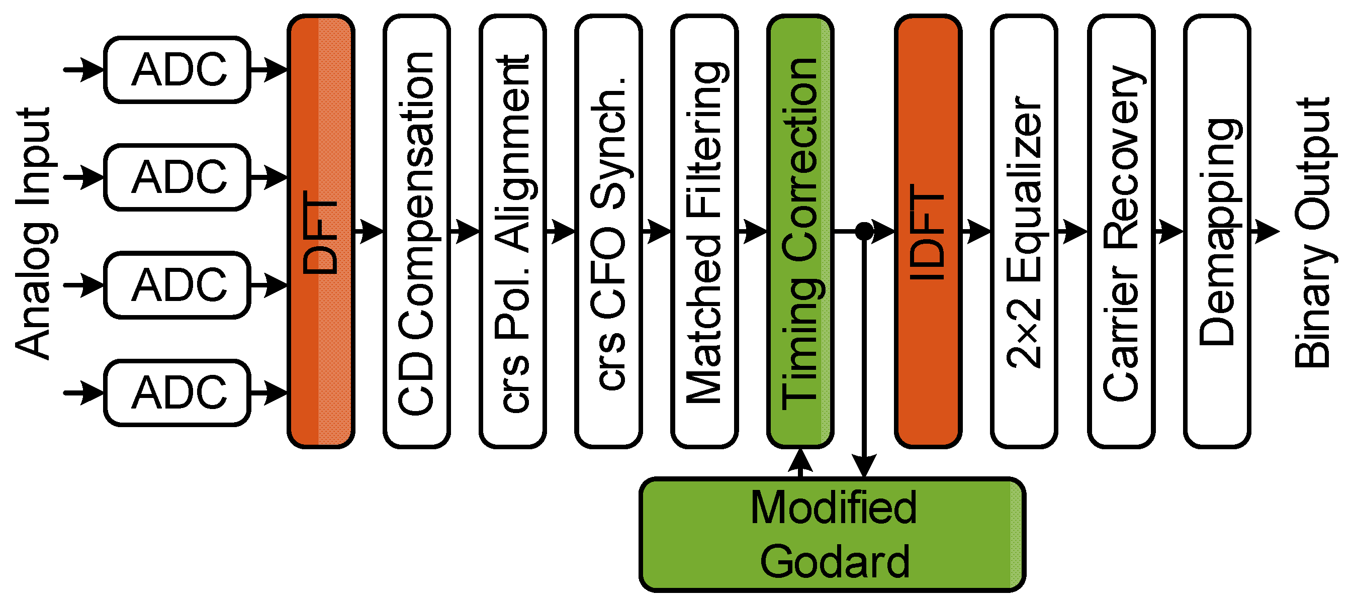
The proposed coherent signal processing structure is shown in Figure 1. Four analog-to-digital converters (ADC) convert the analog output of the coherent receiver’s front-end to the digital domain. The four signals correspond to in-phase and quadrature components of x- and y-polarization. These four channels are converted to the frequency domain by a discrete Fourier transform (DFT). For a reliable timing recovery, we apply the following synchronization algorithms beforehand: chromatic dispersion compensation, coarse polarization alignment, coarse carrier frequency offset correction [9], and matched filtering. Then, the timing recovery operates in a feedback loop. The timing recovery consists of the modified Godard estimator and the timing correction block. The timing correction block performs a frequency domain resampling of the signal. After the timing correction, the signal can be downsampled to one sample per symbol. Then an inverse discrete Fourier transform (IDFT) converts the signal back to the time domain. A 2×2 equalizer equalizes the signal and does fine polarization demultiplexing. The carrier recovery corrects the frequency and phase offsets of the signal. Finally, demapping converts the complex symbols back to binary information.
The advantage of frequency domain processing for the timing correction becomes clear when looking at the mathematical operations required for resampling. While resampling in the time domain requires a convolution with a sinc-function, frequency domain processing is much simpler. Here, a time shift corresponds to applying a linearly increasing phase shift as a function of frequency. The phase slope describes the strength of the timing shift. This is explained by Equation (1).
Here, is the Fourier transform of the time domain signal , and is the time shift.
The implementation complexity of Equation (1) is influenced by two aspects. First, a variable digital filter is needed to handle the varying time shift. Second, downsampling to one sample per symbol is needed for the final symbol decision. When performing the timing recovery in the time domain, an efficient implementation for the variable digital filter is the Farrow structure [10]. Here, a change in results in an update of only one scalar value, whereas in the general case, all finite impulse response (FIR) filter coefficients have to be adapted with respect to the time shift. The filter coefficients could be determined with the Lagrange interpolation, however this brings in some band limitation [11]. Additionally, when the conversion factor for the downsampling to one sample per symbol is a ratio of very large integers, fractional delay filters become difficult to implement and computationally expensive [12]. The increased complexity results out of the higher amount of filter coefficients that are needed to sustain a desired performance.
However, in the frequency domain, oversampling factors consisting of large integers can be efficiently handled by adapting the ratio of DFT to IDFT size. The delay with a certain time shift is done by manipulating the phase according to Equation (1).
Further insights on the tracking of chromatic dispersion (CD), polarization, and coarse carrier frequency offset (CFO) can be found in [13]. Here, we observed that the clock tone gives insight on how to synchronize these impairments.
3. Multiplier-Free Modified Godard Timing Recovery
The Godard algorithm is a technique that estimates the timing error of a signal with at least two samples per symbol based on frequency domain coefficients [6]. Equation (2) shows an adaption of the discretized representation as used in [14].
Here, is the discrete Fourier transform of the received time domain signal , is the size of the DFT, and is the complex conjugate.
By calculating the imaginary part of this CT (as shown in Equation (3)), the Godard technique is realized.
The estimate follows a sinusoidal shape, which is commonly referred to as an s-curve (see Section 4 for further details). For positive estimates, the samples were taken too late with respect to the symbols, while for negative estimates, the samples were taken too early. Due to the sinusoidal shape, there is no unique correspondence between the timing error and the value of the estimate. As a result, this scheme cannot be used for feedforward structures. For feedback structures, the sign of the estimate can be used to control a feedback loop. The loop operates towards the zero crossing of the estimate between too late and too early and therefore the ideal sampling phase. When calculating the angle instead of the imaginary part, a linear dependence between the timing error and the estimate can be observed. A normalization by provides the estimate for a feedforward timing correction.
3.1. Modified Godard Algorithm for Simplified Clock Tone Calculation
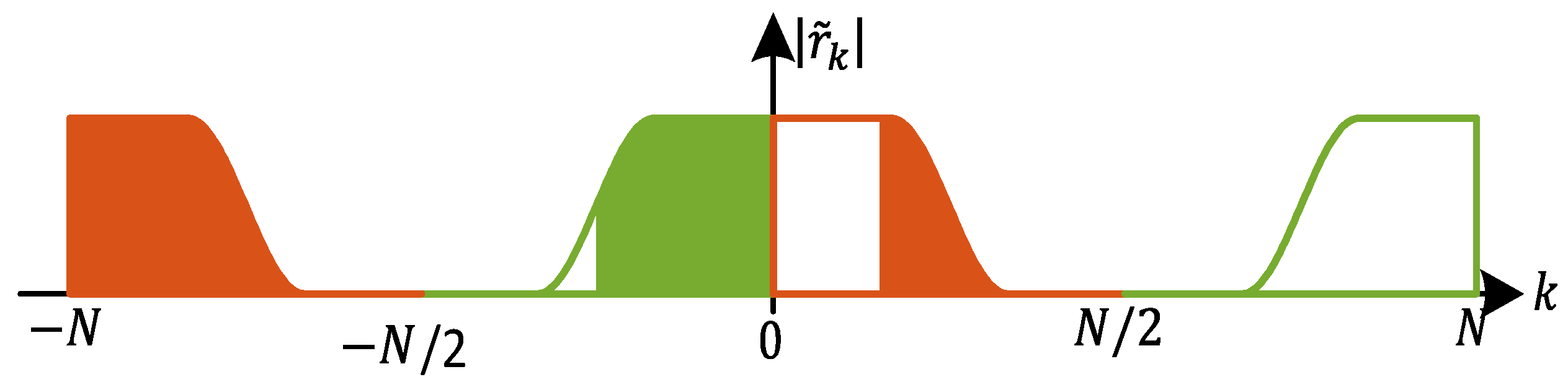
The clock tone calculation can be simplified. To illustrate the necessary steps, we start with Figure 2 that shows a graphical representation of the DFT coefficients used to calculate the Godard estimate. The Godard algorithm multiplies the positive frequency components (upper sideband, red part in Figure 2) with the complex conjugate of the negative frequency components (lower sideband, green part in Figure 2). Note that the DFT spectrum is periodic, so that the coefficients and are equal.
Figure 2 displays a spectrum from to . Commonly, a spectrum is displayed from to . In the following derivations, we will display the spectrum from to for explanatory reasons.
The Godard algorithm can be improved in two steps, resulting in the modified Godard technique. In the first step, terms that do not contribute to the timing estimate are neglected. In the second step, the algorithm is adapted to arbitrary oversampling, which allows for operation with less than two samples per symbol.
For the first step, we simplify Equation (3) by dropping terms in the summation that only give negligible contributions. To illustrate this process, we show it graphically in Figure 3. Here, the magnitude of and is displayed in Figure 3a,b, respectively. Figure 3c shows the overlap of both spectral parts and their multiplication according to Equation (3) in blue. This illustrates that only some elements provide meaningful contributions to the timing estimate. The other elements are zero in magnitude and only contaminate the estimate with additional noise. Moreover, it can be seen that it is sufficient to calculate the sum from to , because the sum from to would only add a factor of two.
With the first adaption of neglecting the terms without information, the estimation of the timing error changes to Equation (4).
Consequently, the size of the area (see the blue in Figure 3c) depends on the roll-off factor and therefore the excess bandwidth. It is interesting to note that Godard has already discussed band-pass filtering of the signal sidebands for a practical implementation. Such a band-pass filtering corresponds to a reduction of the summation limits as elaborated above. Limiting the summation by the excess bandwidth was also discussed in [15].
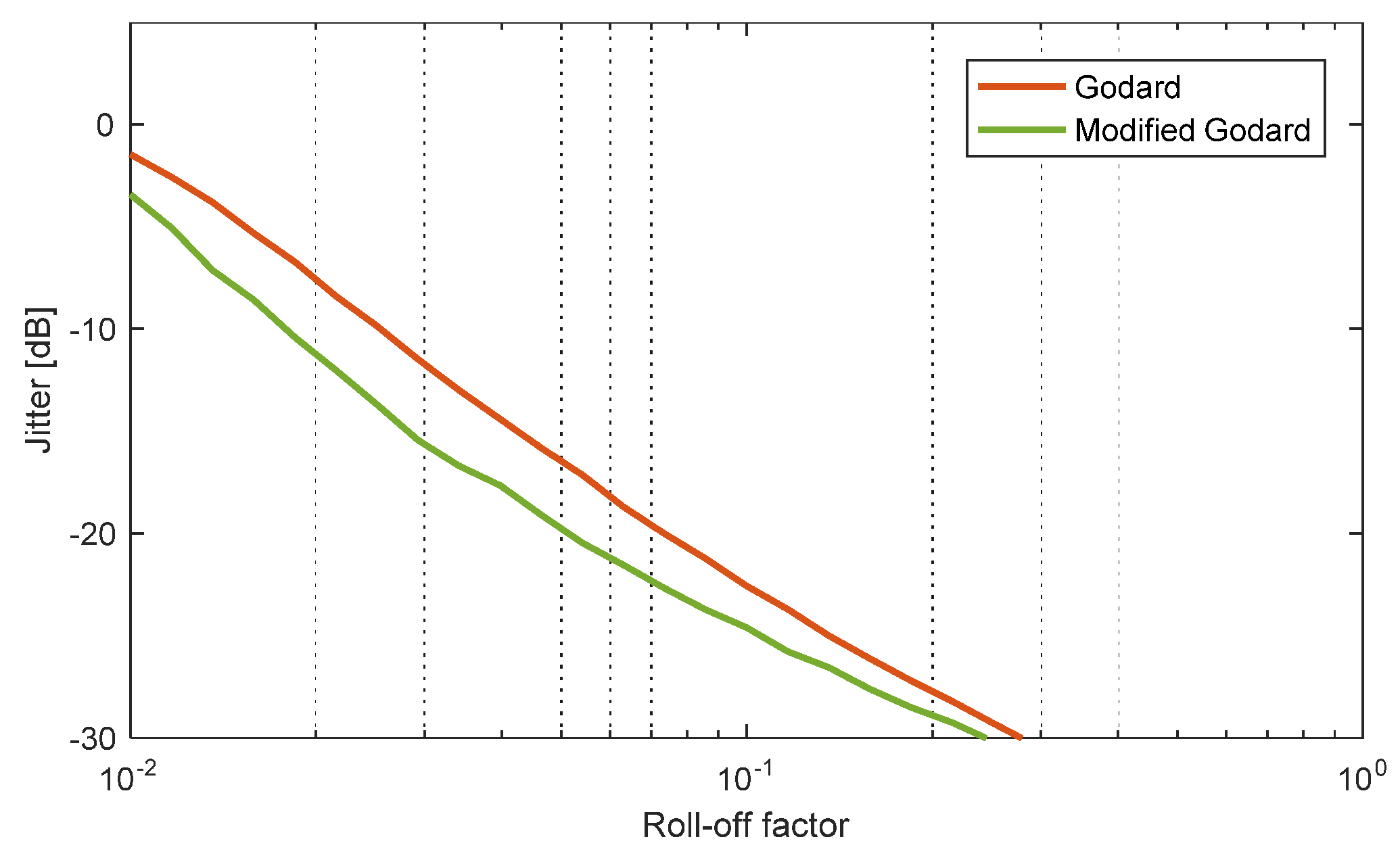
To evaluate the influence of the adaption on performance, we use the variance of the timing estimation error in logarithmic scale. This so-called jitter is calculated from the fluctuations of the estimate around the actual value. The calculated jitter is displayed in Figure 4. The red curve shows the jitter over roll-off factor for the original Godard technique, and the green curve shows that for the modified Godard technique. It can be seen that the modified Godard technique has a reduced jitter, especially for smaller roll-off factors. For larger roll-off factors, the modified Godard algorithm converges to the original Godard algorithm. Therefore, it can be summarized that neglecting the outer elements reduces the amount of computational steps, but nevertheless improves the performance of the estimate.
The second step takes the amount of oversampling of the processed signal into account. This is illustrated in Figure 5, where the oversampling is reduced from 2 to 4/3. The original Godard technique would fail in this situation because it requires two samples per symbol. However, when overlapping the red and green half of the spectrum as displayed in Figure 5c, the estimate for the timing error can still be calculated.
This adaption brings us to:
, , and should be chosen in a way such that the lower and upper bound of the summation results in an integer number.
Without oversampling (), the roll-off factor would have to be zero and so the sum would no longer contain any elements. Therefore, and is required for timing error estimation in the frequency domain. The same limitation occurs for a duobinary signal [16]; here too, no elements would be left in the summation.
3.2. Multiplier-Free Modified Godard Algorithm
Reducing the number of required multiplications typically leads to a reduced computational complexity. So far, Equation (5) has complex multiplications per timing error estimate. Now, we substitute these multiplications with an approximation. For this, we adapt to Equation (6) were we perform the calculation in polar coordinates.
Calculating the imaginary part results in:
In a hardware implementation, the multiplier-free CORDIC algorithm performs the transformation from Cartesian to polar coordinates [17].
Our investigations revealed that neglecting the magnitude of Equation (7) does not significantly decrease the performance of the modified Godard algorithm, but simplifies the calculation. Therefore, we can calculate the timing estimate as described in Equation (8).
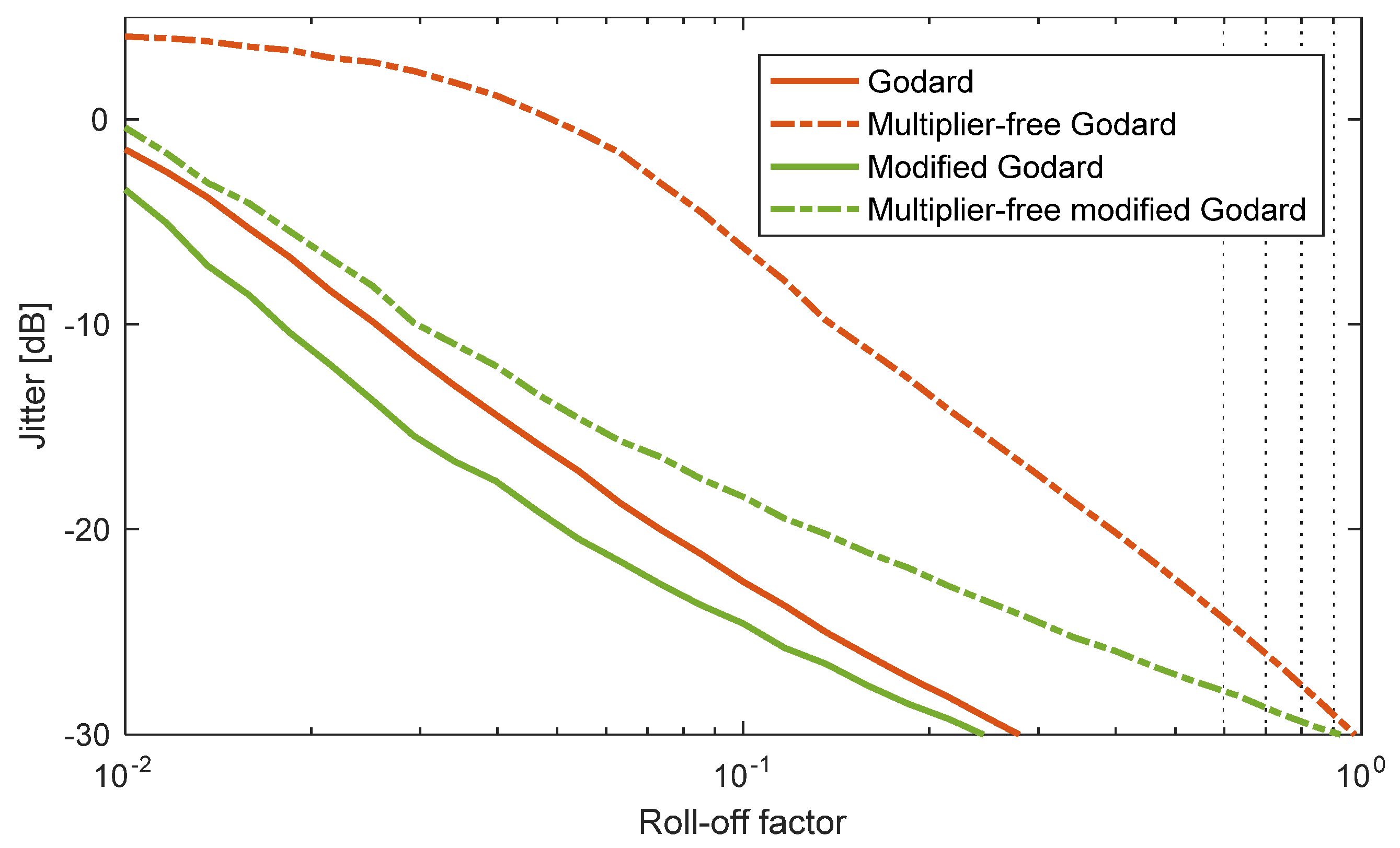
The influence of neglecting the amplitude can be seen in Figure 6. Neglecting the amplitude results in a severe performance decrease for the original Godard (see red dashed curve). The reason for this is that the elements with zero magnitude, which we neglected for the modified Godard algorithm, now have the same influence as the elements that contain the phase information. This clearly decreases performance. Since, for the modified Godard, we only consider elements that are of interest, the amplitude neglect does not have a big influence.
For the feedback loop, we are only interested in the zero crossing of the estimate. For this reason, the first Taylor expansion of the sine function can be used (see Equation (9)). This adaption eliminates the last computationally heavy calculation, and we are only left with additions.
4. Comparison of the Modified Godard Algorithm to the Gardner Algorithm
In this section, the timing estimation algorithms are extended to include the Gardner algorithms. For this, we first comment on how timing jitter can be determined, and then compare the different versions of the Godard algorithm from above with the two versions of the Gardner algorithm.
Timing jitter can be calculated from the statistics of the zero crossing of the s-curve (see Figure 7) [7,18]. This can be achieved in four steps. First, we resample the signal to several sets with a different timing offset. Second, we evaluate the timing estimate with a feedback algorithm. Third, we fit a sinusoidal to the estimates. Fourth, we determine the zero crossing of the sinusoidal. This zero crossing will have zero mean, and its variance gives a quantitative estimate of the timing jitter. The timing jitter can be calculated with Equation (10):
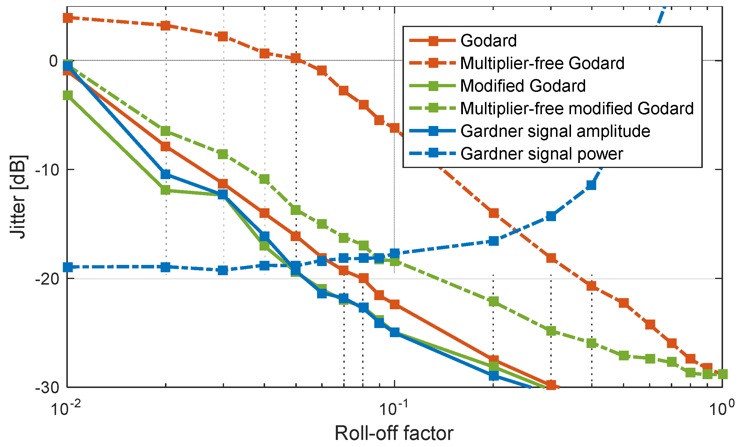
The Gardner algorithm can be used in two ways. It can be applied to the signal amplitude [1] as well as the signal power [18]. Figure 8 shows the jitter over roll-off factor of six different timing estimation algorithms for a 16QAM signal with an SNR of 16.5 dB. The six different algorithms consist of different versions of the Godard algorithm as well as the two Gardner algorithms. It can be seen that the Gardner algorithm with the signal amplitude lies in the range of the Godard and modified Godard algorithms. The Gardner algorithm applied to the signal power provides the lowest jitter for signals with roll-off factors smaller than 0.05.
Our simulations show that the result of Figure 8 applies to a wide range of modulation formats and SNRs, and will only result in an increased timing jitter for the Gardner algorithm applied to the signal power when switching to more advanced modulation formats or decreasing the SNR.
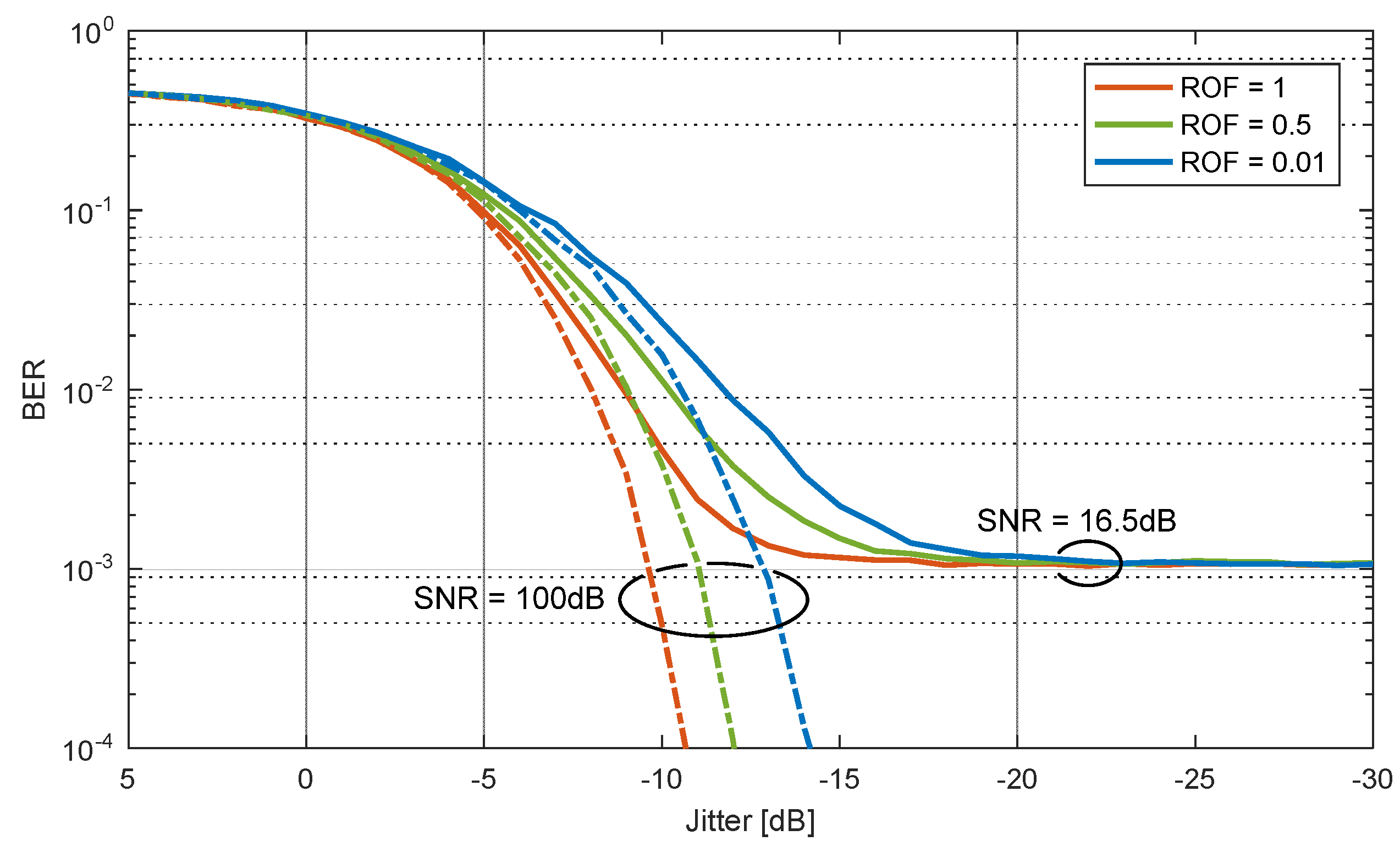
Next, we will determine the BER for a certain timing jitter. To simulate the timing jitter, we used a normal distribution with zero mean and a variance according to the desired timing jitter. This distribution was used to resample the signal and measure the resulting BER afterwards. Figure 9 shows the resulting BER for different timing jitter values. A 16QAM signal with a roll-off factor of 1, 0.5, and 0.01 is simulated. The signals are evaluated with an SNR of 100 dB and an SNR of 16.5 dB. It can be seen that a signal with a roll-off factor of 1 is most resilient to timing jitter. When operating at a BER of 10−3, the signal quality below a timing jitter of −20 dB is dominated by the SNR. Therefore, a timing jitter below −20 dB does not bring benefit to the signal quality.
The timing jitter has a different impact on signals with different modulation formats. The higher the order of the modulation format, the stronger the impact of the timing jitter. Figure 10 shows the BER over timing jitter for a signal with roll-off factor of 0.1 and quadrature phase-shift keying (QPSK), 16QAM, and 64QAM as modulation formats. As expected, it can be seen that QPSK is more robust to timing jitter than 16QAM and 64QAM.
The values in Figure 9 and Figure 10 were obtained without averaging the timing jitter. Since the estimates are unbiased and the drift of the timing estimate over time is rather small, averaging the estimates will reduce the jitter significantly. With these considerations, timing jitters above −20 dB will also allow an operation at a BER of 10−3.
5. Realization of Multiplier-Free Modified Godard on Real-Time Platform
To estimate the complexity of a hardware implementation, the multiplier-free modified Godard algorithm derived above was implemented in very high speed integrated circuit (VHSIC) hardware description language (VHDL) and tested with Xilinx Vivado and Mentor Graphics ModelSim. For comparison to a pure time domain algorithm, we implemented the Gardner algorithm. The Gardner algorithm is seen as a candidate for next-generation receivers [19].
The hardware design is realized for an oversampling of 4/3, a clock frequency of 250 MHz, 96 symbols per clock cycle (=24 GBd), and 6 bit resolution. Table 1 compares the modified Godard hardware requirements of the implementation in Xilinx Vivado with a Gardner synchronization in the time domain.
When compared to the frequency domain, the time domain adaptive FIR filter for timing correction requires 22 times more lookup tables, 6 times more flip-flops, and an additional 2016 DSP slices for multiplications. Additionally, to the estimate and correction, as listed in Table 1, roughly 36% of the lookup tables (LUT) and 18% of the flip-flops (FF) would be required for the transformation to the frequency domain and the transformation to polar coordinates. However, the DFT transformation is needed for CD compensation and other equalization stages anyway, and the polar transformation greatly simplifies the CD compensation as well.
To test the performance of the timing synchronization loop, a signal with a certain timing error was generated in Matlab and sent to the test bench in ModelSim. To test the dynamic and the static response of the loop, the test signal was impaired for the first 8 µs with a sampling frequency offset of 50 kHz, and for the following 8 µs the sampling frequency offset was set to zero (red curve in Figure 11). From the line plotted in green, one can see how the modified Godard algorithm corrects the timing error. After 2 µs settling time, the 50 kHz sampling frequency offset is tracked successfully. The offset between introduced and corrected error results from the latency between error estimation and correction. For all tested modulation formats (QPSK, 8QAM, and 16QAM, depicted as insets in Figure 11), the same synchronization loop behavior was observed. Therefore, the performance is independent of the modulation format.
6. Performance Evaluation in Experiment
Finally, we show the performance difference between the six timing estimation algorithms (see Figure 8) for signals with different roll-off factors based on experimental results. To this end, a DP-16QAM signal with 32 GBd and a varying roll-off factor was measured. To enable a roll-off factor between 0.01 and 1, an oversampling of two was used for all of the evaluated signals.
Figure 12 shows the experimental setup. DP-16QAM signals with the desired pulse-shape (roll-off factor 0.01–1.0) and random data with a length of 219 bits were generated offline. The in-phase and quadrature parts for both polarizations of the signal were converted to the analog domain by four digital-to-analog converters (DAC) with a sampling rate of 64 GSa/s and 20 GHz electrical bandwidth. The output of the DACs was used to modulate the signal laser with a dual-polarization in-phase and quadrature (IQ) modulator. Noise was added to reach the desired BER of 10−3. A coherent receiver consisting of a 90° hybrid with four balanced detectors and four analog-to-digital converters (ADC) with 32 GHz electrical bandwidth received the optical signal. Finally, offline processing was used to evaluate the signal and determine the roll-off dependence of the compared algorithms.
The frequency domain signal processing chain described in Figure 1 was used to evaluate the received signal. Since a transmission over a longer distance would not give further insight to the comparison of the timing estimation algorithms, the CD correction step could be skipped for our comparison. Figure 13 shows the jitter over roll-off factor for the two versions of Godard, modified Godard, and Gardner timing estimation algorithms. These findings match our simulations that were presented before (see Figure 4).
7. Conclusions
A modified Godard timing estimation algorithm that allows for fast and efficient timing estimation has been introduced. It enables operation with less than two samples per symbol, which is not possible with the original Godard technique. The algorithm outperforms the multiplier-free Godard by, e.g., showing an improvement of more than 10 dB in jitter tolerance for a roll-off of 0.1. When compared to an implementation of the Gardner algorithm with the signal power, the newly introduced algorithm comes at the price of a slightly higher jitter for small roll-off factors, but pays off by allowing operation without any multiplications, an overall complexity reduction by more than a factor of two, and a factor of 22 and 6 times less LUTs and flip-flop operations, respectively.
Acknowledgments
We acknowledge financial support by the European Commission under the FP7 program, project FOX-C (grant No. 318415), by the Xilinx University Program (XUP), and Oclaro for lending the optical modulators. It is a pleasure to acknowledge stimulating discussion with W. Blumer, C. Hafner, and A. Messner.
Author Contributions
Arne Josten conceived the concept, performed the simulations and the measurement, analyzed the data, and wrote the manuscript. Benedikt Baeuerle developed the signal processing architecture, the hardware architecture, and the measurement, and helped with the manuscript. Edwin Dornbierer and Jonathan Boesser realized the VHDL implementation of the algorithms. David Hillerkuss organized the required hardware and wrote the manuscript. Juerg Leuthold conceived the concept, designed the experiment, and wrote the manuscript.
Conflicts of Interest
The authors declare no conflict of interest.
References
- Gardner, F.M. A bpsk/qpsk timing-error detector for sampled receivers. IEEE Trans. Commun. 1986, 34, 423–429. [Google Scholar] [CrossRef]
- Alexander, J.D.H. Clock recovery from random binary signals. Electron. Lett. 1975, 11, 541–542. [Google Scholar] [CrossRef]
- Mueller, K.; Muller, M. Timing recovery in digital synchronous data receivers. IEEE Trans. Commun. 1976, 24, 516–531. [Google Scholar] [CrossRef]
- Oerder, M.; Meyr, H. Digital filter and square timing recovery. IEEE Trans. Commun. 1988, 36, 605–612. [Google Scholar] [CrossRef]
- Seung Joon, L. A new non-data-aided feedforward symbol timing estimator using two samples per symbol. IEEE Commun. Lett. 2002, 6, 205–207. [Google Scholar] [CrossRef]
- Godard, D. Passband timing recovery in an all-digital modem receiver. IEEE Trans. Commun. 1978, 26, 517–523. [Google Scholar] [CrossRef]
- Huang, L.; Wang, D.; Lau, A.P.T.; Lu, C.; He, S. Performance analysis of blind timing phase estimators for digital coherent receivers. Opt. Express 2014, 22, 6749–6763. [Google Scholar] [CrossRef] [PubMed]
- Josten, A.; Baeuerle, B.; Dornbierer, E.; Boesser, J.; Abrecht, F.; Hillerkuss, D.; Leuthold, J. Multiplier-Free Real-Time Timing Recovery Algorithm in the Frequency Domain Based on Modified Godard. In Proceedings of the Signal Processing in Photonic Communications, Boston, MA, USA, 27 June–1 July 2015; Optical Society of America: Boston, MA, USA, 2015. [Google Scholar]
- Zhou, X. Efficient clock and carrier recovery algorithms for single-carrier coherent optical systems: A systematic review on challenges and recent progress. IEEE Signal Process. Mag. 2014, 31, 35–45. [Google Scholar] [CrossRef]
- Farrow, C.W. A continuously variable digital delay element. In Proceedings of the IEEE International Symposium on Circuits and Systems, Espoo, Finland, 7–9 June 1988; IEEE: New York, NY, USA, 1988; Volume 2643, pp. 2641–2645. [Google Scholar]
- Diaz-Carmona, J.; Dolecek, G.J. Applications of Matlab in Science and Engineering—Fractional Delay Digital Filters; INTECH Open Access Publisher: Rijeka, Croatia, 2011. [Google Scholar]
- Mitra, S. Digital Signal Processing; McGraw-Hill Education: New York, NY, USA, 2010. [Google Scholar]
- Josten, A.; Baeuerle, B.; Song, M.; Pincemin, E.; Hillerkuss, D.; Leuthold, J. Modified Godard algorithm applied on a fractional oversampled signal to correct cd, polarization, and cfo. In Proceedings of the Signal Processing in Photonic Communications, Vancouver, BC, Canada, 18–20 July 2016; Optical Society of America: Boston, MA, USA, 2016. [Google Scholar]
- Sun, H.; Wu, K.-T. A novel dispersion and pmd tolerant clock phase detector for coherent transmission systems. In Proceedings of the Optical Fiber Communication Conference and Exposition (OFC/NFOEC), Los Angeles, CA, USA, 6–10 March 2011. [Google Scholar]
- Stojanovic, N.; Chuan, H. Clock recovery in coherent optical receivers. In Proceedings of the Photonic Networks, 12. ITG Symposium, Leipzig, Germany, 2–3 May 2011; Optical Society of America: Los Angeles, CA, USA, 2012. [Google Scholar]
- Li, J.; Tipsuwannakul, E.; Eriksson, T.; Karlsson, M.; Andrekson, P.A. Approaching nyquist limit in wdm systems by low-complexity receiver-side duobinary shaping. J. Lightwave Tech. 2012, 30, 1664–1676. [Google Scholar] [CrossRef]
- Volder, J.E. The cordic trigonometric computing technique. IRE Trans. Electron. Comput. 1959, 8, 330–334. [Google Scholar] [CrossRef]
- Yan, M.; Tao, Z.; Dou, L.; Li, L.; Zhao, Y.; Hoshida, T.; Rasmussen, J.C. Digital clock recovery algorithm for nyquist signal. In Proceedings of the Optical Fiber Communication Conference/National Fiber Optic Engineers Conference 2013, Anaheim, CA, USA, 17–21 March 2013; Optical Society of America: Los Angeles, CA, USA, 2013. [Google Scholar]
- Kikuchi, N.; Yano, T.; Riu, H.R. Fpga prototyping of single-polarization 112-gb/s transceiver for optical multilevel signaling with intensity and delay detection. J. Lightwave Tech. 2016, 34, 1762–1769. [Google Scholar] [CrossRef]
Figure 1.
Overview of the receiver signal processing chain with the timing synchronization in the frequency domain. Four analog-to-digital converters (ADC) sample the analog input. A discrete Fourier transform (DFT) converts the signal to the frequency domain. Subsequently, the synchronization blocks for chromatic dispersion (CD) compensation, coarse (crs) polarization alignment, coarse carrier frequency offset (CFO) synchronization, and matched filtering are applied. Then, the timing synchronization feedback loop estimates and corrects the sampling phase offset. An inverse discrete Fourier transform (IDFT) converts the signal back to the time domain. A 2 × 2 equalizer separates the two polarizations and equalizes the signal. A carrier recovery corrects for frequency and phase offsets. Finally, demapping converts the complex symbols to binary information. DFT: discrete Fourier transform, IDFT: inverse discrete Fourier transform.

Figure 2.
Illustration of the magnitude of typical DFT coefficients needed to calculate the Godard timing error estimate. The DFT spectrum is periodic. The upper sideband is colored in red and the lower sideband is colored in green.
Figure 2.
Illustration of the magnitude of typical DFT coefficients needed to calculate the Godard timing error estimate. The DFT spectrum is periodic. The upper sideband is colored in red and the lower sideband is colored in green.

Figure 3.
First adaption towards the modified Godard algorithm by neglecting unnecessary terms. (a) Shows the magnitude of the coefficients of a twofold oversampled, raised-cosine spectrum with roll-off factor 1/3. (b) Shows the spectrum shifted by . (c) Shows the overlap of and and in blue their multiplication. It can be seen that elements of the multiplication are zero and so negligible.
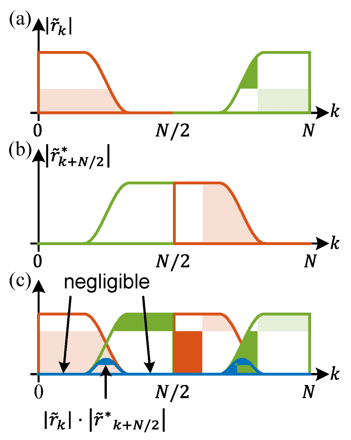
Figure 4.
Simulation results for the jitter over roll-off factor. The results of the Godard algorithm (red) and modified Godard algorithm (green) are shown. (M = 16QAM quadrature amplitude modulation, amount of evaluated symbols per roll-off factor equals 51.2 million, random data, DFT size 1024, oversampling of 2, SNR = 16.5 dB); QAM: quadrature amplitude modulation; SNR: signal-to-noise ratio.

Figure 5.
Second simplification towards the modified Godard algorithm by adapting the shift to the amount of oversampling. (a) Shows the coefficients of an oversampled, raised-cosine (RC) spectrum with roll-off factor 1/3. (b) Shows the spectrum shifted by . (c) Shows the overlap of and . The multiplication is only calculated in the area of to . Even though the oversampling is reduced to below two, the estimate can still be calculated.
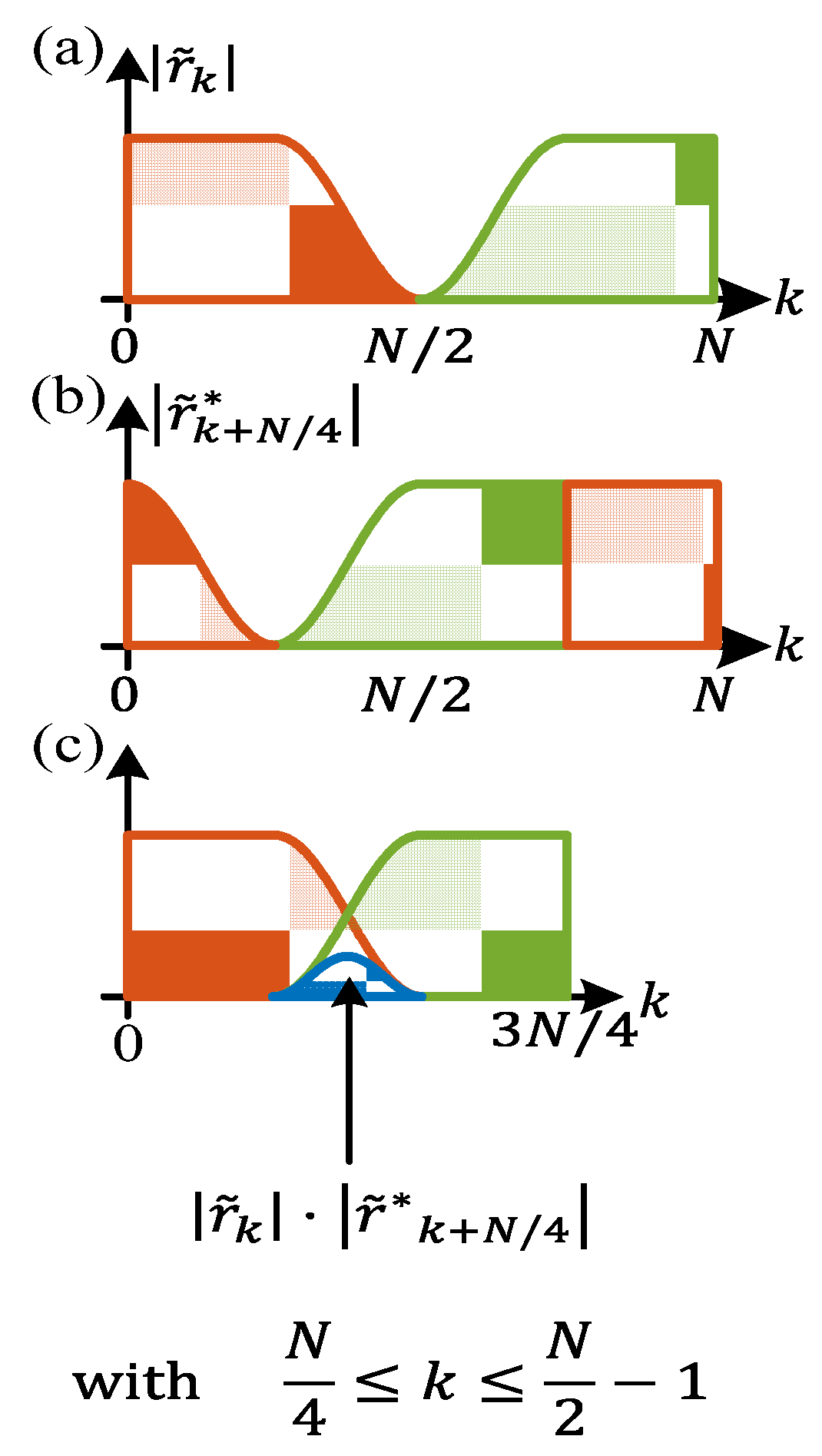
Figure 6.
Simulation results for the jitter over roll-off factor for Godard and modified Godard and the multiplier-free version. (Signals with an oversampling of two, 16QAM, and SNR = 16.5 dB were simulated).
Figure 6.
Simulation results for the jitter over roll-off factor for Godard and modified Godard and the multiplier-free version. (Signals with an oversampling of two, 16QAM, and SNR = 16.5 dB were simulated).

Figure 7.
S-curve for a signal with 16QAM, SNR = 16.5 dB, and roll-off factor of 0.1, 6 million symbols were simulated. The s-curve shows the response of a feedback timing estimation algorithm (Gardner algorithm in this case) to a signal with a timing error varying between −0.5 and 0.5. The color indicates the probability of occurrence. The jitter corresponds to the distribution of the zero crossing.
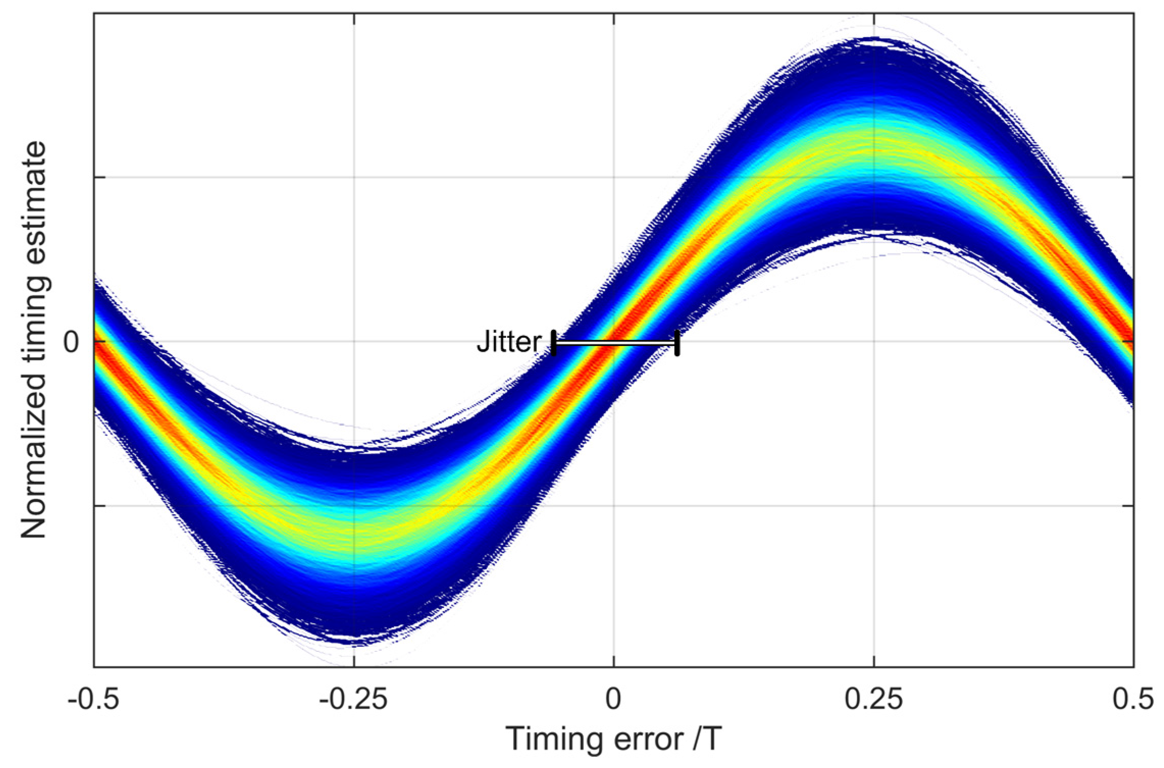
Figure 8.
Jitter over roll-off factor for a signal with 16QAM with an SNR of 16.5 dB (BER = 10−3). BER: bit-error ratio
Figure 8.
Jitter over roll-off factor for a signal with 16QAM with an SNR of 16.5 dB (BER = 10−3). BER: bit-error ratio
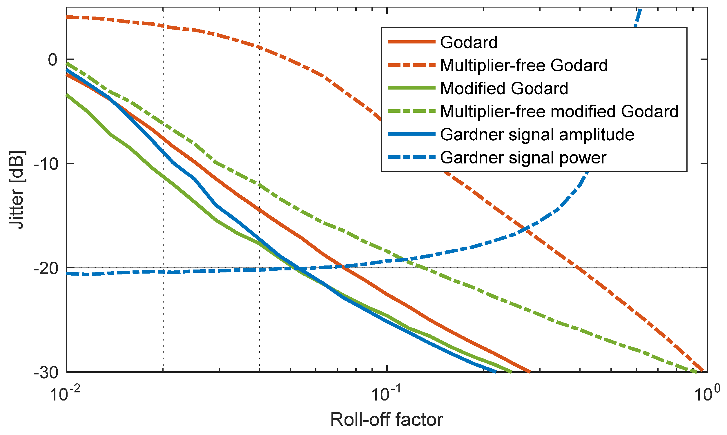
Figure 9.
BER over jitter for a signal with 16QAM with different roll-off factors. The results for an SNR of 100 dB and 16.5 dB are shown.
Figure 9.
BER over jitter for a signal with 16QAM with different roll-off factors. The results for an SNR of 100 dB and 16.5 dB are shown.

Figure 10.
BER over roll-off factor for a signal with roll-off factor 0.1 and modulation formats of QPSK (blue), 16QAM (red), and 64QAM (yellow) are shown. The results are plotted for an SNR of 100 dB and 9.8 dB, 16.5 dB, 22.5 dB, respectively; QPSK: quadrature phase-shift keying.
Figure 10.
BER over roll-off factor for a signal with roll-off factor 0.1 and modulation formats of QPSK (blue), 16QAM (red), and 64QAM (yellow) are shown. The results are plotted for an SNR of 100 dB and 9.8 dB, 16.5 dB, 22.5 dB, respectively; QPSK: quadrature phase-shift keying.
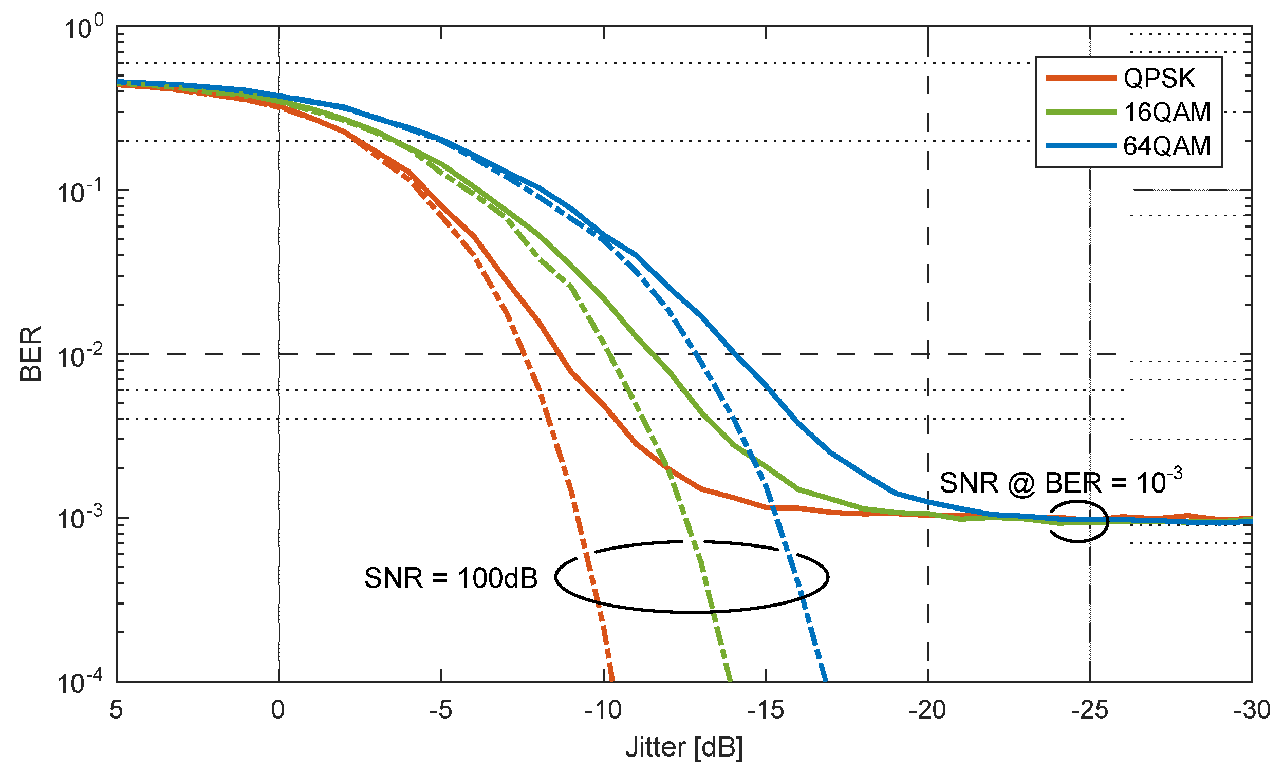
Figure 11.
ModelSim analysis of the timing correction (SNR = 10 dB, 16QAM, n = 4/3, = 1/3, sampling frequency offset 50 kHz). Insets show constellation diagrams with timing error and QPSK, 8QAM, and 16QAM after timing synchronization for a BER of 10−3.
Figure 11.
ModelSim analysis of the timing correction (SNR = 10 dB, 16QAM, n = 4/3, = 1/3, sampling frequency offset 50 kHz). Insets show constellation diagrams with timing error and QPSK, 8QAM, and 16QAM after timing synchronization for a BER of 10−3.
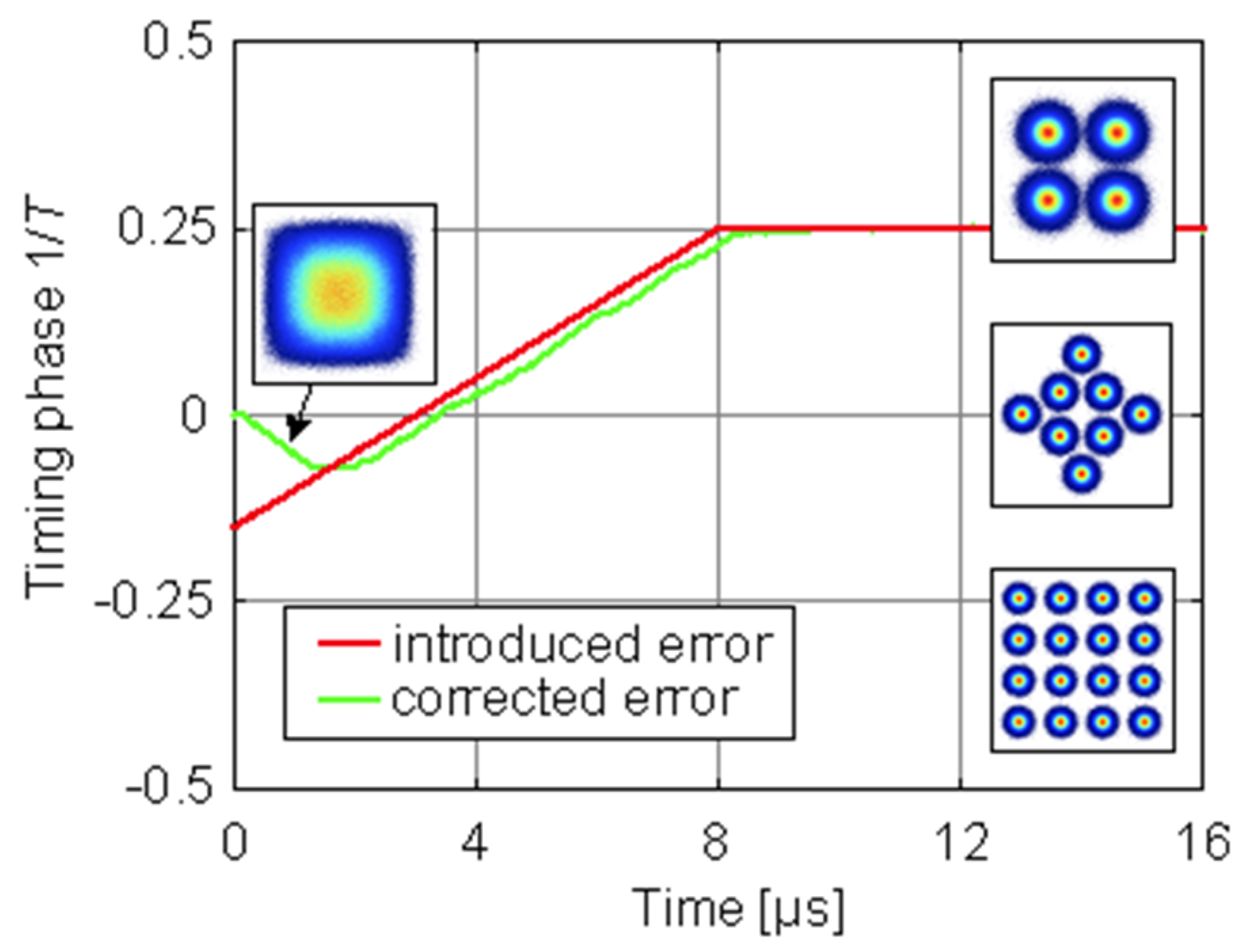
Figure 12.
Overview of measurement setup. The transmitter consists of offline signal generation, four digital-to-analog converters (DAC), and a laser being modulated with a dual-polarization in-phase and quadrature (IQ) modulator. Noise was added to reach the desired BER. A coherent receiver with a local oscillator (LO) and four channels with balanced detectors and analog-to-digital converters is used to receive the signal. The detected signal is evaluated in offline digital signal processing (DSP).
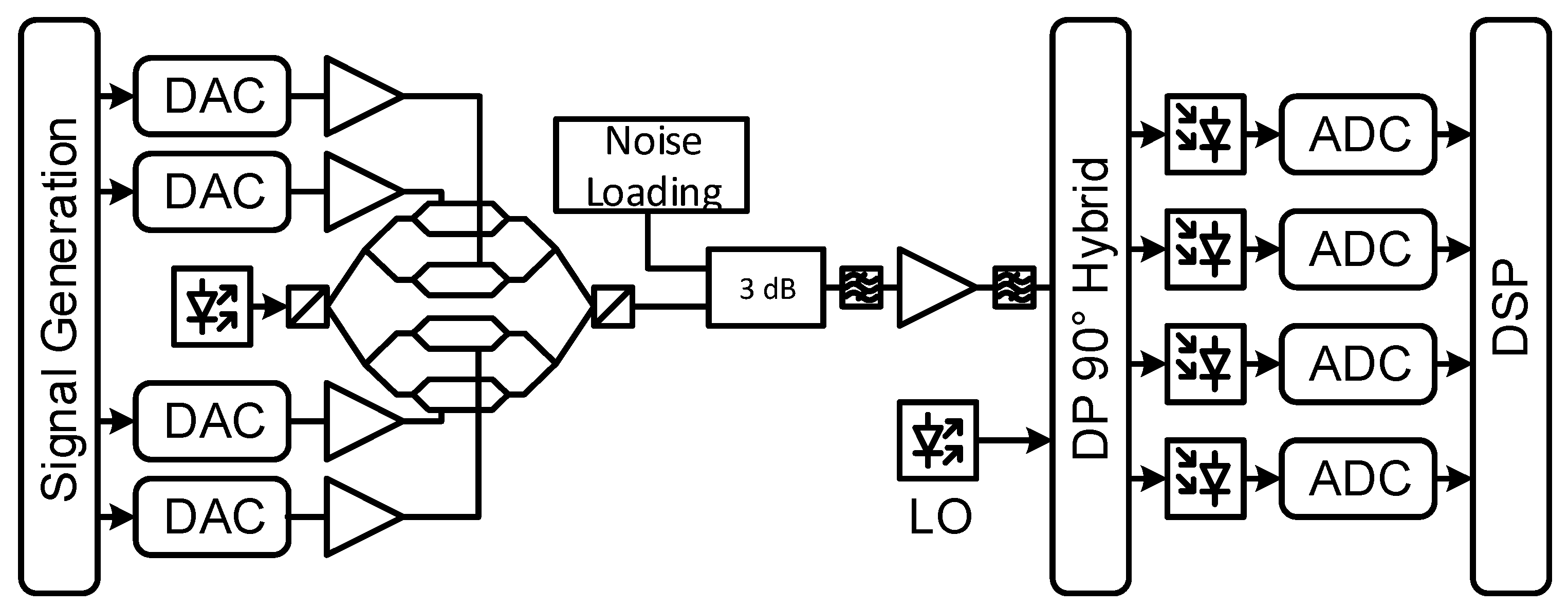
Figure 13.
Measurement results for timing jitter over roll-off factor. (M = 16QAM, 32 GBd, amount of symbols per roll-off factor 0.5 million, fast Fourier transform (FFT) size 1024).
Figure 13.
Measurement results for timing jitter over roll-off factor. (M = 16QAM, 32 GBd, amount of symbols per roll-off factor 0.5 million, fast Fourier transform (FFT) size 1024).


Table 1.
Hardware requirements for Gardner and modified Godard algorithms (Percentages are given with respect to the Xilinx Virtex 7 xc7vx690t board).
Table 1.
Hardware requirements for Gardner and modified Godard algorithms (Percentages are given with respect to the Xilinx Virtex 7 xc7vx690t board).
| Algorithm | Gardner | Modified Godard | ||
|---|---|---|---|---|
| Estimation | Correction | Estimation | Correction | |
| Lookup tables | 1435 (<1%) | 35,652 (8%) | 694 (<1%) | 1612 (<1%) |
| Flip-flops | 1932 (<1%) | 78,280 (9%) | 871 (<1%) | 11,641 (1%) |
| DSP | 97 (3%) | 2016 (56%) | 0 (0%) | 0 (0%) |
© 2017 by the authors. Licensee MDPI, Basel, Switzerland. This article is an open access article distributed under the terms and conditions of the Creative Commons Attribution (CC BY) license (http://creativecommons.org/licenses/by/4.0/).
Share and Cite
MDPI and ACS Style
Josten, A.; Baeuerle, B.; Dornbierer, E.; Boesser, J.; Hillerkuss, D.; Leuthold, J. Modified Godard Timing Recovery for Non Integer Oversampling Receivers. Appl. Sci. 2017, 7, 655. https://doi.org/10.3390/app7070655
AMA Style
Josten A, Baeuerle B, Dornbierer E, Boesser J, Hillerkuss D, Leuthold J. Modified Godard Timing Recovery for Non Integer Oversampling Receivers. Applied Sciences. 2017; 7(7):655. https://doi.org/10.3390/app7070655
Chicago/Turabian StyleJosten, Arne, Benedikt Baeuerle, Edwin Dornbierer, Jonathan Boesser, David Hillerkuss, and Juerg Leuthold. 2017. "Modified Godard Timing Recovery for Non Integer Oversampling Receivers" Applied Sciences 7, no. 7: 655. https://doi.org/10.3390/app7070655
Note that from the first issue of 2016, this journal uses article numbers instead of page numbers. See further details here.