
Analysis of Land Cover Classification Using Multi-Wavelength LiDAR System


Department of Civil Engineering, National Chiao Tung University, Hsinchu 30010, Taiwan
*
Author to whom correspondence should be addressed.
Appl. Sci. 2017, 7(7), 663; https://doi.org/10.3390/app7070663
Submission received: 26 April 2017
/
Revised: 22 June 2017
/
Accepted: 26 June 2017
/
Published: 28 June 2017
(This article belongs to the Special Issue Laser Scanning)
Abstract
:Featured Application
The featured application of this study is to combine the geometrical and spectral features from advanced multi-wavelength LiDAR in land cover classification.
Abstract
The airborne multi-wavelength light detection and ranging (LiDAR) system measures different wavelengths simultaneously and usually includes two or more active channels in infrared and green to acquire both topographic and hydrographic information. The reflected multi-wavelength energy can also be used to identify different land covers based on physical properties of materials. This study explored the benefits of multi-wavelength LiDAR in object-based land cover classification, focusing on three major issues: (1) the evaluation of single- and multi-wavelength LiDARs for land cover classification; (2) the performance of spectral and geometrical features extracted from multi-wavelength LiDAR; and (3) the comparison of the vegetation index derived from active multi-wavelength LiDAR and passive multispectral images. The three-wavelength test data were acquired by Optech Titan in green, near-infrared, and mid-infrared channels, and the reference data were acquired from Worldview-3 image. The experimental results show that the multi-wavelength LiDAR provided higher accuracy than single-wavelength LiDAR in land cover classification, with an overall accuracy improvement rate about 4–14 percentage points. The spectral features performed better compared to geometrical features for grass, road, and bare soil classes, and the overall accuracy improvement is about 29 percentage points. The results also demonstrated the vegetation indices from Worldview-3 and Optech Titan have similar characteristics, with correlations reaching 0.68 to 0.89. Overall, the multi-wavelength LiDAR system improves the accuracy of land cover classification because this system provides more spectral information than traditional single-wavelength LiDAR.
1. Introduction
1.1. Motivation
Airborne light detection and ranging (LiDAR), also known as airborne laser scanning (ALS), is the one of the most important technologies to obtain three-dimensional (3D) information effectively. The lidar system acquires high-resolution topographic data including (3D) shape and backscattered energy. LiDAR data provide both geometrical and radiometrical information to identify different objects, and it has been extensively used in various applications, for example digital elevation modeling [1], topographic mapping [2], 3D object modeling [3], and land cover classification [4,5].
Land cover classification is an important task for understanding natural resources as well as land resource management. Because of the demand for land cover information, various land cover maps are available online with different spatial resolutions, for example, the European Space Agency (ESA) 300 m global land cover map (GlobCover) [6] and 30 m global land cover data (GlobeLand30) [7]. The land cover map can be derived from active or passive sensors using an unsupervised classification system such as ISODATA and supervised classification such as Support Vector Machines (SVM). Several studies reported land cover classification using airborne LiDAR data, which provide 3D shape information rather than 2D spectrum information in classification. Moreover, the penetration of LiDAR also improves the ability to identify vegetation. The LiDAR features for land cover classification can be based on geometrical, waveform, and intensity features. In addition, LiDAR data and multispectral images can be combined to gain both shape and spectrum information [4].
Most commercial airborne LiDAR systems are commonly monochromatic or dual-wavelength laser systems, recording either discrete signals or full waveform signals. The monochromatic LiDAR system, such as topographic LiDAR, utilizes fixed wavelength laser (e.g., 1064 nm in near-infrared (NIR)) to acquire the return signal from the target. The dual-wavelength LiDAR system is capable of measuring two different wavelengths (e.g., 532 nm in green and 1064 nm in NIR) simultaneously. One of the well-known dual-wavelength LiDAR system is bathymetric LiDAR, which uses an NIR laser to determine water surface and a corresponding green laser to determine the underwater terrain. Bathymetric LiDAR can collect shallow-water terrain based on the NIR and green lasers. To enhance the applications of LiDAR system, a different type of multi-wavelength LiDAR system has been developed (such as Optech Titan, Riegl VQ-880-G, and Leica Chiroptera II) that acquires more 3D points than the monochromatic LiDAR system and also offers physical properties of material (such as backscattered energy) in different wavelengths. Backscattered energy from active sensors is a kind of physical property from different targets, mainly dependent on target materials, target roughness, and laser wavelength. Multi-wavelength LiDAR utilizes different wavelengths to obtain backscattered energies to separate different land covers. Therefore, understanding the capability of the multi-wavelength LiDAR system (also called multispectral LiDAR) is an important subject in the development of LiDAR technology.
1.2. Previous Studies
Several studies show the advantages of multi-wavelength LiDAR data in different applications, such as atmospheric processing [8,9], geological analysis [10], fire detection [11], topographic mapping [12,13,14], map updating [15], and plant monitoring [16,17]. Bakula, (2015) [18] analyzed the accuracies of digital terrain models (DTMs) from Optech Titan and showed that the mean differences among DTM generation from three channels were less than 0.03 m, and the composition of the three intensities could be considered an alternative orthoimage product. Bakula et al. (2016) [19] also used the Optech Titan multispectral LiDAR and maximum likelihood classifier in land covers classification, achieving an overall accuracy of 90% for six classes. Fernandez-Diaz et al. (2016) [20] presented the capabilities of assessment and performance metrics for the multi-wavelength LiDAR to quantify the performance of Optech Titan multi-wavelength LiDAR system in land cover classification, bathymetric mapping, canopy characterization, and geometrical accuracy. Zou et al. (2016) [21] used Optech Titan multi-wavelength LiDAR data to perform object-based land cover classification and found that a pseudo normalized difference vegetation index (pNDVI) generated from a multi-wavelength LiDAR system may improve vegetation identification, achieving an overall accuracy higher than 90% and kappa coefficient reaching 0.89. Sun et al. (2017) [22] compared the reflectance of active multispectral LiDAR, active hyperspectral LiDAR, and passive spectrometer for leaf nitrogen concentration; their coefficient of determination (R2) for spectrometer (R2 = 0.73) and hyperspectral LiDAR (R2 = 0.74) showed a high correlation with leaf nitrogen content. Based on previous studies, the multi-wavelength LiDAR not only increases the number of 3D points but also provides backscattered energies in different wavelengths.
Geospatial object-based image analysis (GEOBIA) [23] has been widely applied in multispectral images to merge similar pixels into a region; the geometrical and radiometrical properties of regions are then extracted to separate different land covers. The advantages of object-based classification compared with pixel-based classification have been established in previous studies [24,25]. Through image segmentation, the related image pixels are combined into image objects that provide the objects’ attributes and shape to identify different land covers [26]. Object-based classification is therefore more flexible than traditional pixel-based classification. A similar process can be applied to object-based LiDAR classification [27]. To obtain useful information in LiDAR classification, the LiDAR data are clustered into an object, and its features are then selected to separate different land covers in object-based LiDAR classification.
1.3. Need for Further Study
Multi-wavelength or multispectral LiDAR is an advanced sensor in the development of LiDAR technology. Several researchers studied the capability and benefit of using multispectral LiDAR in different applications, mostly focusing on the features from multi-wavelength LiDAR itself, but the comparison of measurements based on active multispectral LiDAR and passive multispectral image are sparse. This study explores the benefits and limitations of different aspects of land cover classification, including the comparison of single- and multi-wavelength LiDARs, the spectral and geometrical features, and the similarity of NDVI between an active multi-wavelength LiDAR system and a passive multispectral image.
1.4. Research Purpose
The aim of this research was to analyze the results of land cover classification using multi-wavelength LiDAR and compare the vegetation features from active multi-wavelength LiDAR and passive multispectral images. The geospatial object-based image analysis (GEOBIA) was used to achieve land cover classification. The multi-wavelength LiDAR was from Optech Titan using 532 nm (green), 1064 nm (NIR), and 1550 nm (MIR), whereas the multispectral image is from Worldview-3 (WV-3) satellite multispectral images. This study adopted the object-based image classification approach, a proposed scheme including feature extraction, image segmentation, and object-based classification. The correctness and completeness were generated by manual interpretation and verified by comparing LiDAR and multispectral images. The analysis compared (1) the results from single-wavelength LiDAR and multi-wavelength LiDAR; (2) spectral and geometrical features from multi-wavelength LiDAR system; and (3) LiDAR-derived and image-derived vegetation index.
2. Materials
2.1. Test Area
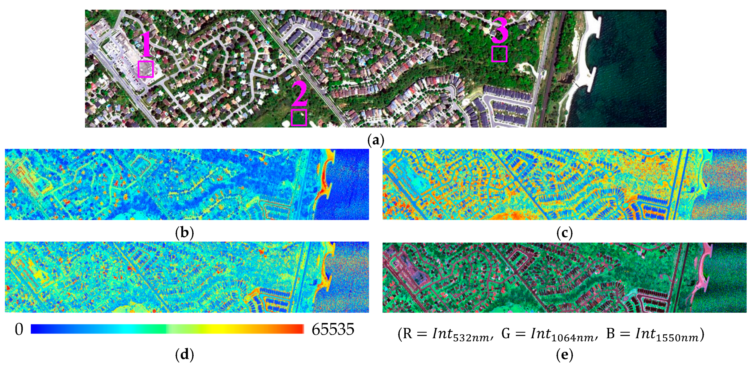
The test area, located at Adams Park, Canada, is about 574,600 m2 (1690 × 340 m) at a geometric elevation ranging from 28 m to 93 m. The park is a suburban area along the shoreline of Lake Ontario that contains both land and water regions (Figure 1a), and the land cover includes buildings, roads, trees, grass, and bare soil.
2.2. Multi-Wavelength LiDAR
The multi-wavelength LiDAR data were acquired in September 2014 by Optech Titan, a system that includes three active imaging channels at 532 nm visible (green), 1064 nm (NIR), and 1550 nm (MIR) [28]. The flying height is about 400 m. Number of flying strips is three, all merged into a single LAS file. The preprocessing of multi-wavelength LiDAR removes noise points (e.g., air point). Because system parameters and trajectories were limited or unavailable, this study used the intensities from LiDAR’s standard product, which is the amplitude of the return reflection without intensity calibration. Both topographic and hydrographic data for spatial mapping can be obtained from the Titan system from these three channels. We compared the characteristics of the individual laser pulses as well as other characteristics of each channel required to evaluate the behavior and performance of the system (Table 1).
These three intensities with wavelengths of 532 nm, 1064 nm, and 1550 nm (Figure 1b–d) were stored in separated files according to the ASPRS LAS standard. The tested data contained about 14,731,124, 13,530,547, and 12,439,573 points from these three channels, respectively. The total number of points in the study area was about 40 million, and the average point density was about 70.7 pts/m2.
Point density is an important factor in LiDAR processing. In general, three channels in different look directions may acquire more points than one channel. One advantage of multi-wavelength LiDAR is the ability to increase the number of points in a single strip. The scanning angles of the Titan system were designed in different directions to avoid interference and obtain more points. We selected three sub-regions to compare the point densities for different land covers (Table 2), including simple man-made objects, mixed objects, and complex tree regions (boxes 1, 2, and 3 in Figure 1a). Each sub-region is about 2500 m2 (50 × 50 m). In comparison to point density of the single wavelength system, the additional wavelengths in the three wavelengths system (i.e., 1550 nm in 3.5 degree forward; 1550 nm in nadir; 532 nm in 7.0 degree forward) may increase the number of points in the three sub-regions. For building region, the point densities of single wavelength were originally about 23.2–24.8 points/m2 and the use of multi-wavelength LiDAR increased it to 71.5 points/m2. The point density is related to the ability of multiple returns and multi-channel lasers in different scanning directions. This area contains three overlapped flying strips and the tree and building regions were covered by same flying strips. The tree area has a higher penetration rate than buildings and thus produces higher number of multiple returns. A comparison of the tree and building shows that the complex tree region has the highest point density because laser beams from different directions may penetrate the tree crown, demonstrating the benefit of using multi-wavelength LiDAR to improve point density in complex tree regions.
The multi-wavelength LiDAR was rasterized into 0.5 m grid data that included DSMs, DTMs, and intensities from different wavelengths. Because the average point density of the test area was about 70.7 points/m2, the height of DSM was the highest point in the cell, and the intensity map selected the intensity of the highest point in the cell. The ground point for DTM was automatically generated by a non-ground point filtering method in TerraScan Software, and the ground points were then placed into the grid by the kriging interpolation method.
2.3. Multispectral Satellite Image
The reference data are from a WV-3 multispectral satellite image acquired on 21 May 2015. The off-nadir view angle is about 7.8 degrees, and the ground sampling distances for panchromatic and multispectral images are 0.315 m and 1.26 m, respectively. The wavelength of panchromatic image is from 450 nm to 800 nm and contains eight multispectral bands, including coastal (400–450 nm), blue (450–510 nm), green (510–580 nm), yellow (585–625 nm), red (630–690 nm), red edge (705–745 nm), NIR-1 (770–895 nm), and NIR-2 (860–1040 nm) [29]. We manually selected ground control points from multi-wavelength LiDAR and WV-3 image. The registration accuracy of rational function geometrical model is better than one pixel. The DSM from all points was used to generate 0.3 m panchromatic and 1.2 m multispectral orthoimages. We also performed radiometric correction to convert the pixel values to reflectance values [30] using metadata of WV-3 images. The land cover classification only adopted LiDAR features, and the WV-3 satellite image was only a reference image in the selection of training and test regions. In addition, we compared the vegetation indices from the passive WV-3 multispectral image and active multi-wavelength LiDAR.
2.4. Targets of Classification
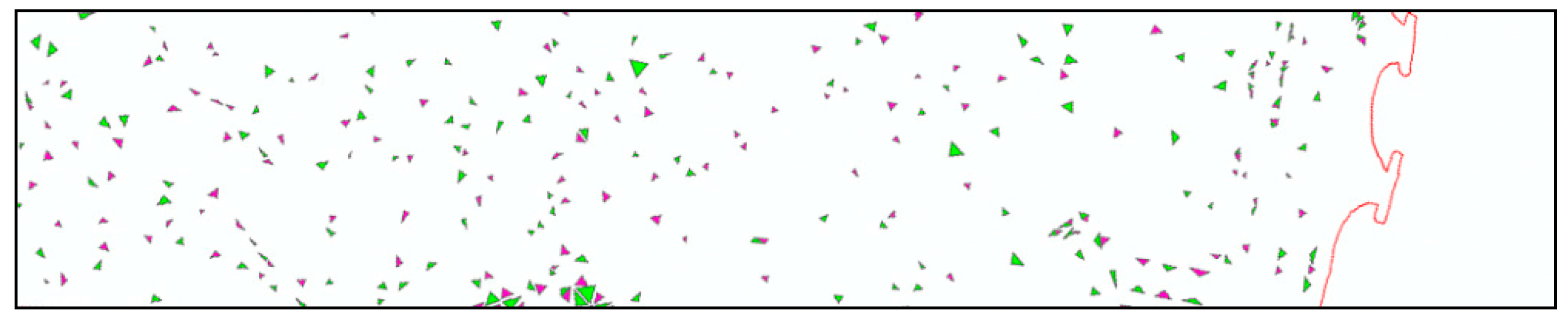
The study area comprises traditional urban types and covers a variety of land cover features on the ground such as buildings, roads, parking lots, shrubs, trees, and open grassy spaces. To define land cover classes in classification, we considered the most important classes for the land cover map and their availability in this study area and selected five major types for classification: buildings, trees, grass, roads, and bare soil. These classes are well-defined land cover types in urban areas and can be identified without ambiguity in reference data. This study manually selected 280 randomly distributed sampling objects comprising 44,158 pixels in the study area. The pixel size was 0.5 × 0.5 m (i.e., the pixel size of rasterized LiDAR), and the area of all selected pixels was 11,039.5 m2. We used 140 objects as the training data and the remaining 140 objects as the test data (Table 3), distributed in areas excluding the water regions (Figure 2).
3. Proposed Scheme
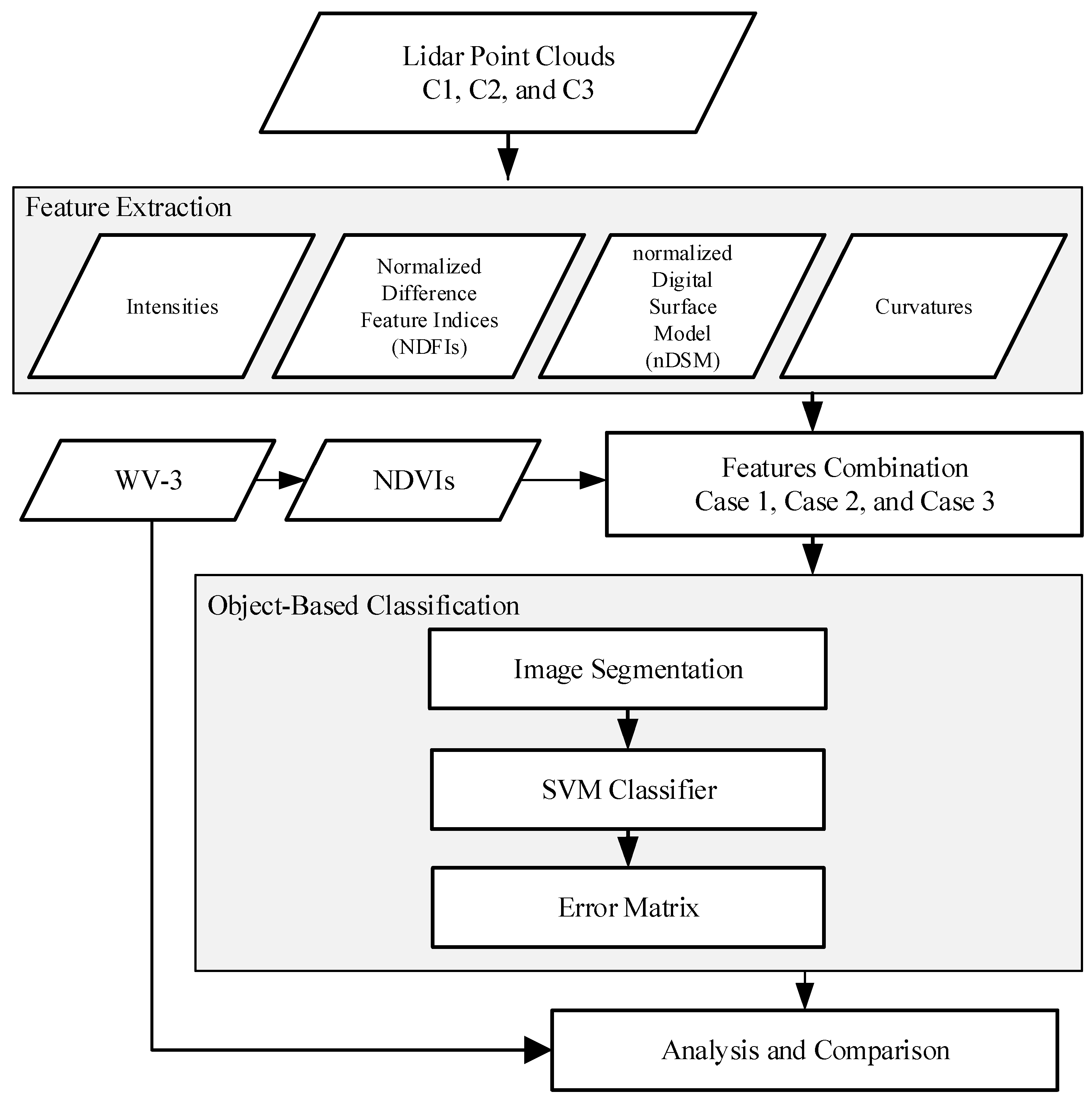
The proposed scheme utilized the concept of geospatial object-based image analysis (GEOBIA) [23] in land cover classification. Figure 3 shows the workflow of proposed scheme. The GEOBIA approach for land cover classification consists of three steps, including feature extraction, image segmentation, and object-based classification. The input data are LiDAR data from different wavelengths, and the preprocessing feature includes extraction, such as geometrical and spectral features. After selecting the training dataset, the object-based classification process applies segmentation and the SVM classifier, and the output data are the classification results from different combinations, including three combinations based on different features (Cases 1 and 2) and different data sources (Case 3). All the combinations used object-based classification to detect land cover types, and the results of all combinations were used to compare the performance of different features.
3.1. Feature Extraction
Feature extraction selects useful information to distinguish different land covers, including spectral and geometrical features from LiDAR. The spectral features selected were intensity and NDFI (Normalized Difference Feature Index), and the geometrical features selected were normalized digital surface model (nDSM) and curvature [31]. The intensities were the amplitude of the return reflection. We used the concept of NDVI to calculate the vegetation index (NDFI) from the spectral characteristics of each channel in the multi-wavelength LiDAR system; the NDFI is used to separate vegetation and non-vegetation from the return signals of active sensor. Because the Optech Titan does not have a red channel, we used the green channel to replace the red channel in NDVI; the infrared channels include NIR and MIR (Equations (1) and (2)). The NDVI from a passive multispectral image was also calculated for comparison (Equations (3) and (4)). The differences between active and passive sensors in the vegetation index were: (1) the return signal of passive signal was reflectance, whereas the return signal of the active signal was backscattered energy; (2) the band width of the passive sensor was comparatively wider than the active sensor.
where is 1550 nm intensity from LiDAR; is 1064 nm intensity from LiDAR; is 532 nm intensity from LiDAR; NIR1 is 772 to 890 nm wavelengths from WV-3; NIR2 is 866 to 954 nm wavelengths from WV-3; and red is 706 to 746 nm wavelengths from WV-3.
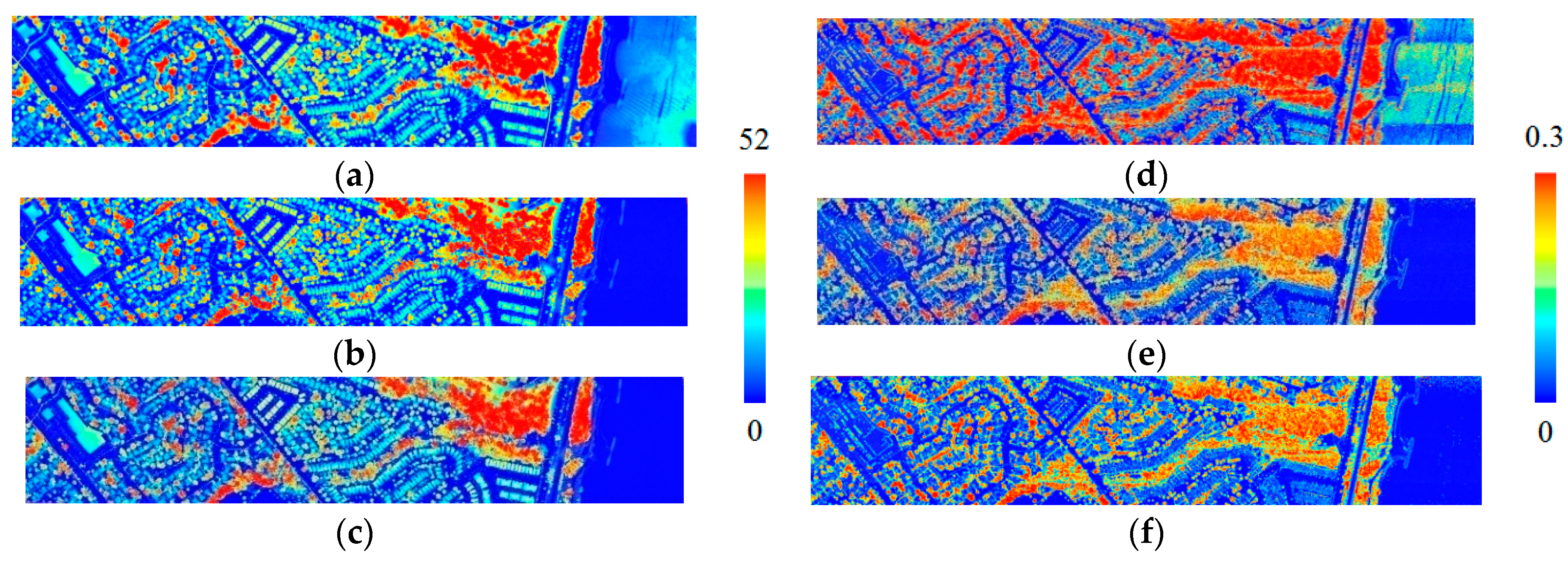
The geometrical features were used to represent the shape and roughness of the LiDAR data. The nDSM represents the object height, obtained by subtracting DTM from DSM. Different objects’ heights can be identified by nDSM. For example, grass and trees have similar spectral responses but different object heights. The curvature, a feature that represents roughness by calculating the spatial eigenvalues of target point clouds and the adjacent points (Equation (5)), is a useful feature to separate objects with smooth and rough surfaces; for example, the roughness of a tree crown is higher than road surface. Curvature is calculated from irregular points within the nearest 50 points and then interpolated into grid data for object classification (Figure 4).
where are the spatial eigenvalues.
3.2. Image Segmentation
The purpose of image segmentation is to generate objects for classification by merging pixels with similar attributes into a region, typically referred to an object. We used the LiDAR features (e.g., intensity, nDSM, curvature) as input data for segmentation, considering both attribute and shape factors. The pixels with similar attributes were merged into an object, and the attributes were the pixel values of the input data. The shape factors were the geometric pattern of the segmented object. The segment criteria are based on the heterogeneity index [32], which combines the attribute and shape factors. Segmentation is a bottom-up method starting from a pixel, and the heterogeneity index is calculated from each pixel as a logical object according to neighborhood pixels. If the heterogeneity index meets the predefined criterion, these pixels are merged.
We implemented image segmentation using Trimble eCognition software (Version 8.7 Trimble Inc., Westminster, CO, USA). All input features used the same coordinate system and pixel size, so different features are overlapped in the same coordinate system for segmentation. We used equal weight for all input features, so all input features have the same impact on segmentation. As the numerical value of all input features are not the same (e.g., nDSM is ranged from 0 m to 50 m while NDFI is ranged from −1 to +1), the range of the value will influence the results of segmentation. This study normalized all the features into the same range. Therefore, all input features have same range of values for segmentation. Segmentation has three parameters, and we used the same empirical parameters for all cases: the segmentation scale was 50, shape was 0.1, and compactness was 0.5. It should be noted that the ideal segmentation parameters for different types of input data might not be the same. We observed the results of segmentation using different parameters to find proper segmentation parameters for this test area. The objective of this study was to compare the results of land cover classification by different features, so we used the same parameters for different types of input data.
3.3. Object-Based Classification
Following segmentation, the object classification stage classifies each object into different land covers based on each object’s spectral and geometrical features. In reality, most land cover is the composition of several similar LiDAR points identified through human interpretation, but identifying the properties of a single LiDAR point is more difficult. The process of object-based classification is more similar to the human interpretation and has been widely used to improve the classification accuracy for remote sensing data [33]. For object-based classification in this study, we used a supervised support vector machine (SVM) designed to handle the complex features by maximizing the margins of hyperplanes using support vectors, and the SVM then classified different features based on training data in the hyperplane. The kernel of SVM in this study was the radial basis function (RBF) [34,35]. To examine the capability of multi-wavelength features, this study used different features in segmentation and classification. Note that the same training and check areas were used in all combinations.
4. Results
The experiments in this study analyzed three different aspects of the validation procedure. The first aspect compares single- and multi-wavelength LiDAR systems. Three channels (i.e., green, NIR, and MIR) were used to simulate single-wavelength LiDAR individually, and the results from single- and multi-wavelength LiDARs were used to compare the accuracy of land cover classification. The second aspect checks the suitability of spectral and geometrical features in land cover classification by evaluating different features extracted from multi-wavelength LiDAR system to understand the significance of the features. The third aspect compares the vegetation indices from passive multispectral images and active multi-wavelength LiDAR, including the results of vegetation classification and correlation of vegetation index.
To quantify the benefits of the multi-wavelength LiDAR system in land cover classification, we used completeness (also called producer accuracy) and correctness (also called user accuracy) for each land cover in different combinations. Completeness measures the percentage of classes occurring in the reference data and errors of omission; by contrast, correctness measures the percentage of extracted classes correctly classified and errors of commission. The confusion/error matrixes for all cases have been placed in the Appendix A.
4.1. Comparison of Single-Wavelength and Multi-Wavelength LiDAR
To compare the accuracy of land cover classification between single- and multi-wavelength LiDAR systems, we designed four combinations (Table 4) including the features intensity, nDSM, and curvature. The first three combinations were single-wavelength LiDAR features from each channel, respectively. The last combination merged all features from three channels, totaling nine, including three intensities, three nDSMs, and three curvatures. The segmentation of single-wavelength LiDAR only considered its own intensity, whereas the segmentation of multi-wavelength LiDAR considered three intensities simultaneously. The classification employed the same training areas but different features.
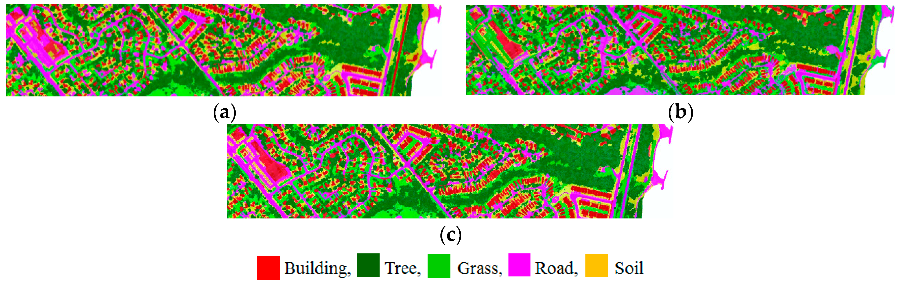
As previously described, the test area was classified into five land cover classes (buildings, trees, grass, roads, and bare soil), and the results from the four combinations were color-coded to indicate each land cover type (Figure 5).
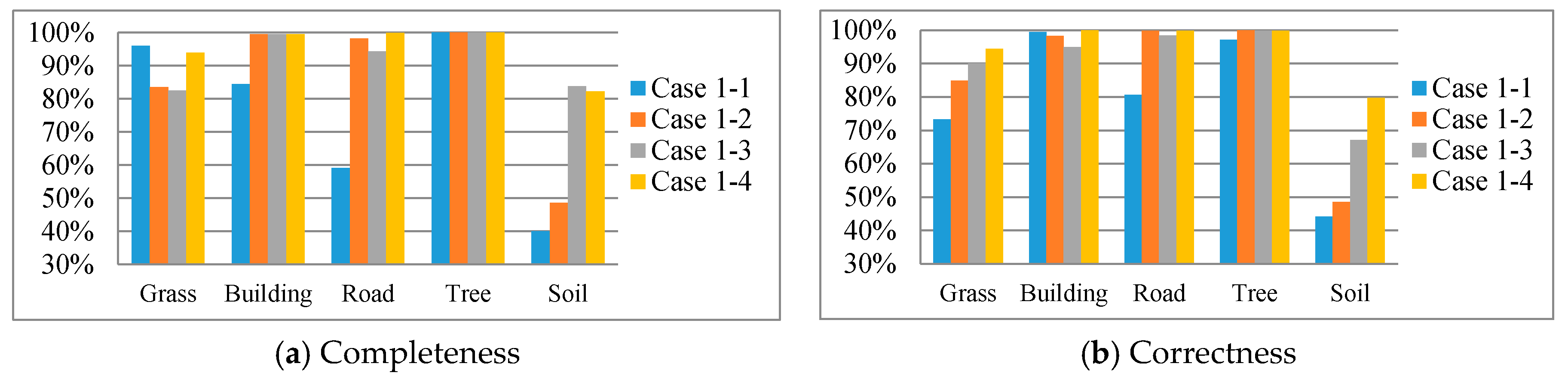
The quantitative results (i.e., completeness and correctness; Table 5 and Figure 6) show that, as expected, the accuracy of the green channel was lower than the other two channels in infrared because the green channel is designed to represent water surface in most situation. The completeness of roads for 532 nm (Case 1-1) was only 59%, lower than other cases, meaning that the infrared channel performs better than the green channel for asphalts road. Therefore, the intensity of infrared is widely used to discriminate between asphalt and non-asphalt roads [36]. The completeness values of bare soil for 532 nm (Case 1-1) and 1064 nm (Case 1-2) were less than 52% because soil, road, and grass have similar height and curvature in the single-wavelength system. The completeness of 1550 nm (Case 1-3) is slightly better than the other two channels because it is near-to-mid infrared. Wang et al. (2012) [8] also found that results from 1550 nm were better than those from 1064 nm. The integration of all features (Case 1-4) provided better discrimination among soil, road, and grass than single-wavelength features.
Because trees and buildings are significantly higher than other land covers, they show limited improvement when the three wavelengths were integrated. Overall, the completeness improvement from single- to multi-wavelength LiDAR ranged from 1.7 to 42.3 percentage points. In correctness analysis, the behavior of soil, road, and grass was similar to results from completeness. The multi-wavelength features (Case 1-4) also improved the correctness of these three classes from 1.4 to 35.8 percentage points. The soil and grass had a higher improvement rate when the multi-wavelength feature was adopted. The decrease in completeness is less than 2.5 percentage points between cases 1-1 and 1-4 for grass. For correctness, the decrease in accuracy is less than 0.2 percentage points between cases 1-2 and 1-4 for tree.
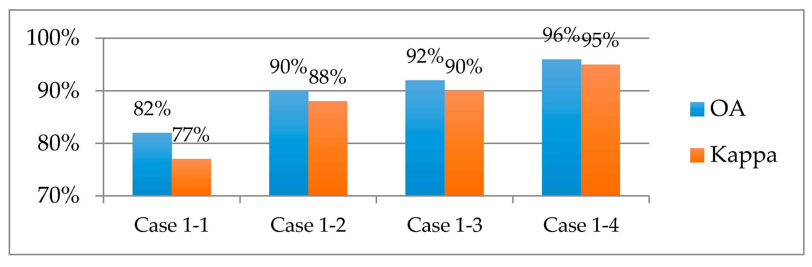
The classification results lead to overall accuracy (OA) from individual channels of 82%, 90%, and 92% from wavelengths 532, 1064, and 1550 nm, respectively. The OA and kappa coefficient achieved 96% and 95%, respectively, using extracted features from the multi-wavelength LiDAR system. The OA of multi-wavelength LiDAR increased 4–14 percentage points compared to single-wavelength LiDAR (Figure 7). The single-wavelength LiDAR extracts limited information and caused misclassifications when the classes had similar reflectivity, such as that for roads and grass in the green channel. The OA of classified results were similar to the features from 1064 nm and 1550 nm (90% and 92%) (Figure 7), but misclassifications still appeared for grass and soil (Figure 6).
4.2. Comparison of Spectral and Geometrical Features from Multi-Wavelength LiDAR
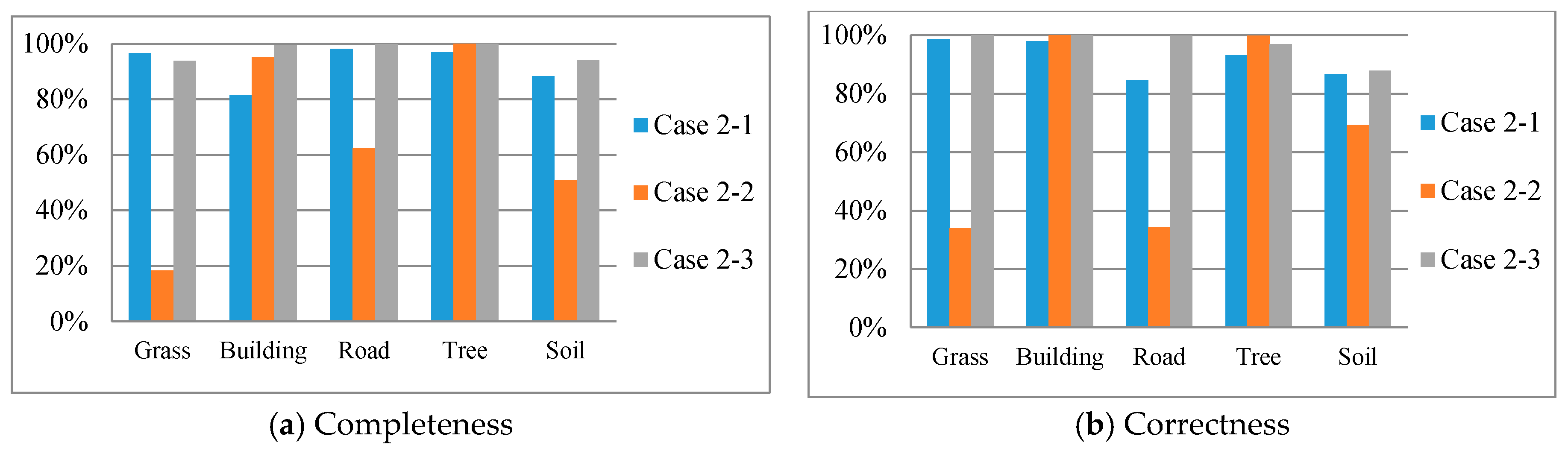
Airborne LiDAR records both 3D coordinates and reflected signals, and the LiDAR points can be used to generate the spectral features (i.e., intensity and vegetation index) and geometrical features (i.e., height and roughness). One characteristic of multi-wavelength LiDAR is providing spectral features at different wavelengths. The spectral feature of multi-wavelength LiDAR is not only the intensity, but also the vegetation index from the infrared and green channels. To compare the capability and benefits of spectral and geometric features for different land cover classification, we designed three combinations (Table 6): spectral features included intensity and NDFIs; geometrical features included nDSM and curvature; and the third merged the features of previous two combinations. For these three cases, the input features for classification were also the features for segmentation, and we used equal weight when combining all these input features in segmentation. We summarized the results of these three cases (Figure 8) and the completeness and correctness for each land cover in different combinations (Table 7, Figure 9).
The completeness from spectral features (Case 2-1) was higher than 80% because road, soil, and grass have different spectral signatures [37]. In addition, the results of spectral features were significantly better than for the geometrical features (Case 2-2) for road, soil, and grass. The geometrical features showed higher accuracy for buildings and trees because these two objects have different roughness (i.e., curvature). Because the heights of grass, road, and soil classes are similar; these geometrical features are not easily discriminated among those objects. The integration of spectral and geometrical features (Case 2-3) improved the accuracy of these three classes from 1.7 to 75.5 percentage points.
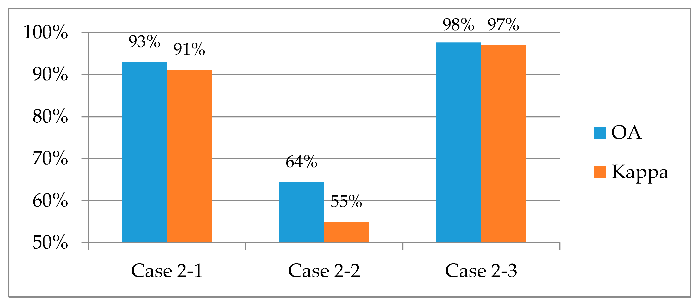
In correctness analysis, the integration of all features (Case 2-3) improved the accuracy from 1.1 to 65.6 percentage points. Most accuracy indices from spectral features were higher than those from geometrical features (Table 7); in other words, the results indicate that the use of LiDAR spectral features contributes more than the geometrical features. The OA of spectral features reaches 93% but only 64% for geometrical features (Figure 10) because of the higher accuracy for buildings and trees but lower accuracy for grasses, roads, and soils. The results demonstrate that spectral features from LiDAR could be useful features in land cover classification when multi-wavelength intensities are available.
4.3. Comparison of Vegetation Index from Active and Passive Sensor
Passive sensors (e.g., optical multispectral images) can only be used to detect naturally available energy (e.g., solar energy). By contrast, active sensors (e.g., LiDAR) provide their own energy source for illumination and obtain data regardless of time of day or season; therefore, active LiDAR sensors are more flexible than optical sensors in different weather conditions. Vegetation detection is an important task in ground-point selection for the digital terrain model (DTM) generation from LiDAR. Traditionally, vegetated areas are detected using the surface roughness from irregular points; intensity from LiDAR data is seldom used in the separation of vegetation and non-vegetation. With the development of multi-wavelength LiDAR, the intensities from different wavelengths are possibly similar to passive sensors in vegetation detection. Our goal is to discover the capability of the vegetation index from LiDAR, and the aim of this section is to compare the performance of vegetation index from active and passive sensors.
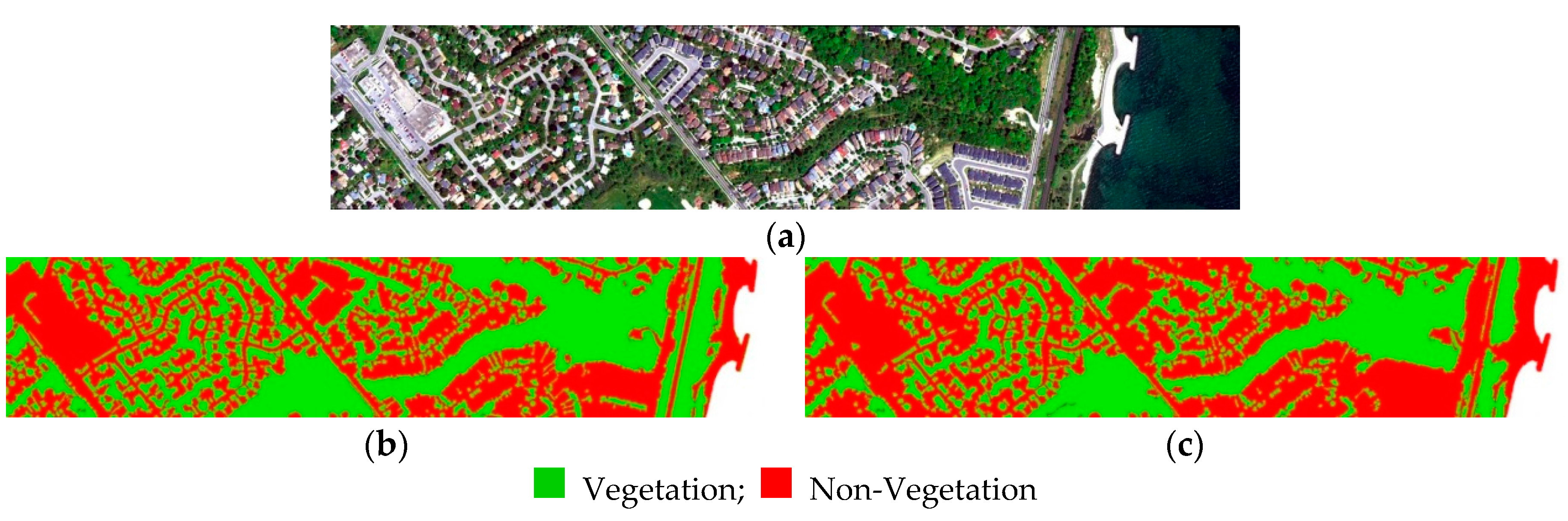
The NDVI has been widely used in vegetation detection, but it is calculated from passive multispectral images. Because the passive sensor has inherent limitations, such as day operation and haze, an active sensor like LiDAR can be operated at night and penetrate haze and might be an option to overcome these restrictions. We designed two cases to analyze the similarity and consistency (Table 8) between vegetation indices from active and passive sensors. Because the reflectance of the multispectral WV-3 image represents the radiance of the object surface (e.g., tree top), we selected the intensity of the highest point in a 1.2 × 1.2 m cell (i.e., pixel size of WV-3 multispectral image) as the LiDAR intensity for LiDAR-derived vegetation index so that both reflectance of the passive sensor and return energy of the active sensor represent the energy of object surface in different wavelengths. For the training and test data, the grass and tree classes were merged into a vegetation class, and the building, road, and soil classes were combined into a non-vegetation class; only the vegetation indices were used in segmentation and classification. A visual comparison of the two results of vegetation detection (Figure 11) show high consistency between these two vegetation indices.
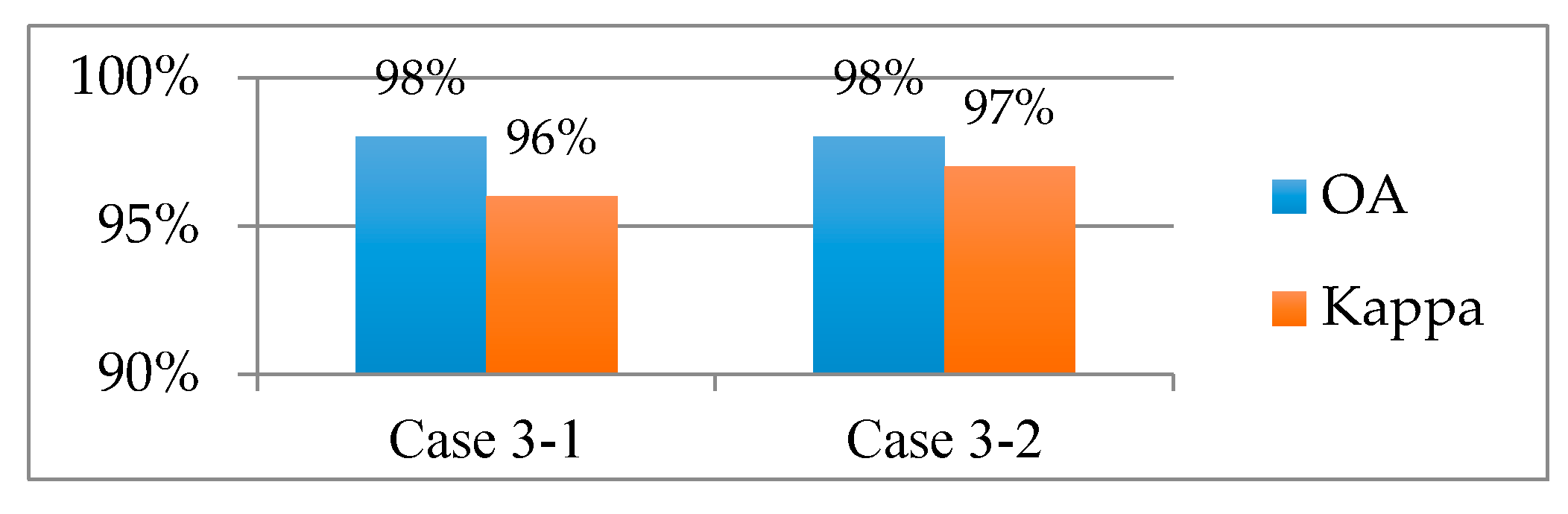
Completeness and correctness were compared between vegetation and non-vegetation in different combinations (Table 9 and Figure 12). Here we considered only two classes: vegetation and non-vegetation; therefore, the results were better than the results in Section 4.1 and Section 4.2 (i.e., five classes). The completeness and correctness analysis for active LiDAR and passive imagery were higher than 96%. The correctness of vegetation detection from the passive sensor was 98% in test samples and slightly lower, 96%, for the active sensor. A small amount of vegetation and non-vegetation was misclassified, but the overall accuracy reached 98% in both cases. The overall accuracies and kappa coefficients were also similar in this test area (Figure 13), with vegetation indices generated from multi-wavelength LiDAR were similar to those from passive multispectral imagery. The kappa of the passive sensor was slightly better (1%) than that for the active sensor. This experiment demonstrated that the vegetation index from active LiDAR sensor could be used to detect vegetation area effectively.
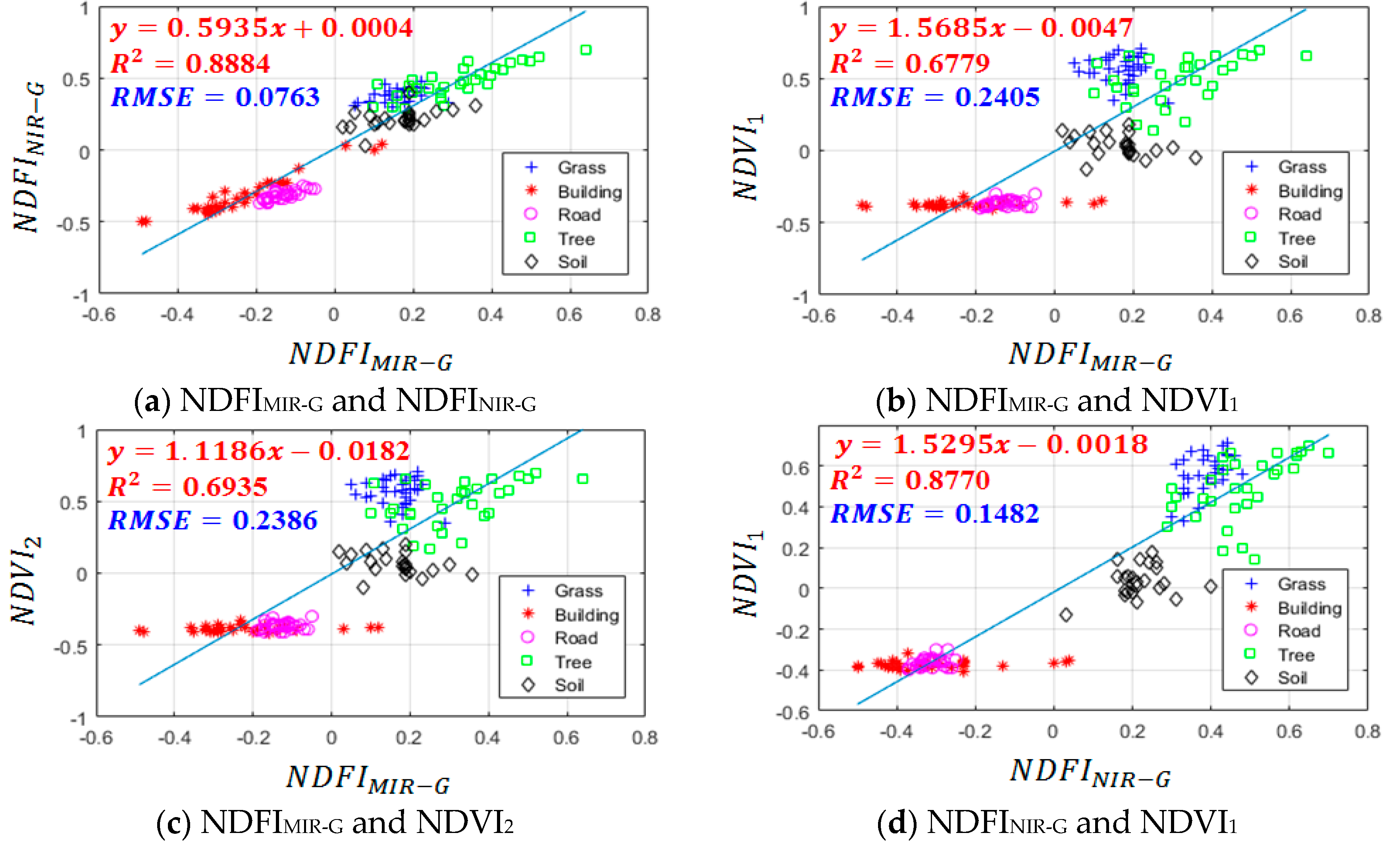
We also used the training data to calculate the coefficient of determination (R2) among these vegetation indices (Figure 14). For each training dataset, four vegetation indices were extracted from both active and passive sensors. Any two vegetation indices were selected to determine the similarity between them, and six combinations were selected for similarity analysis. The R2 between two passive vegetation indices (i.e., NDVI1 and NDVI2) reached 0.99 while the R2 between two active vegetation indices (i.e., NDFIMIR-G and NDFINIR-G) reached 0.88. The R2 among active or passive vegetation indices showed high consistency in these training data.
In the analysis across sensors, the R2 for combinations of (NDFIMIR-G and NDVI1) and (NDFIMIR-G and NDVI2) were less than 0.7 because the NDFIMIR-G used the MIR while the NDVI1 and NDVI2 used NIR. The root-mean-square errors (RMSEs) of (NDFIMIR-G and NDVI1) and (NDFIMIR-G and NDVI2) (i.e., 0.2405 and 0.2386) also had a large fitting error compared to other cases. For NDFINIR-G, NDVI1, and NDVI2, all calculated from NIR, the R2 of combinations (NDFINIR-G and NDVI1) and (NDFINIR-G and NDVI2) were higher than 0.87 for both combinations. Anderson et al. (2016) [38] also found that the vegetation indices from active sensors had high correlations. They reported that the vegetation indices measured from active and passive sensors were correlated (R2 > 0.70) for the same plant species. Although the vegetation index recorded by the active sensor was consistently lower than that of the passive sensor, differences were small and within the range of possibility. In this study, the vegetation indices from active LiDAR were also lower than those from passive imagery and were highly correlated (R2 > 0.87) between active and passive sensors. In addition, the overall accuracy in classification of vegetation from non-vegetation was higher than 98%. Our analysis clearly showed that vegetation indices from multi-wavelength could be a helpful feature for vegetation detection.
5. Conclusions and Future Works
The multi-wavelength LiDAR system is a new technology for obtaining additional spectral information for LiDAR point analysis. This study analyzed the benefits of multi-wavelength LiDAR in land cover classification. Object-based classification is an effective method for land cover classification and vegetation inventory, and this study established an object-based land cover classification scheme using spectral and geometrical features from multi-wavelength LiDAR. The major contributions of this study were to (1) analyze the classification results from single- and multi-wavelength LiDARs; (2) evaluate the improvement rates of different land covers using geometrical and spectral features; and (3) compare the vegetation indices derived from active and passive sensors. The conclusions are summarized as follows:
- (1)
- In the comparison of single- and multi-wavelength LiDARs, the multi-wavelength LiDAR generates more spectral information than the traditional single-wavelength LiDAR. The improvements of OA ranged from 4 to 14 percentage points when multi-wavelength features are available. The spectral features from multi-wavelength LiDAR are useful for the classification of grass, road, and bare soil classes.
- (2)
- In the comparison of geometrical and spectral features, the geometrical features are suitable for identifying objects with different heights and roughness, for example, buildings and trees. spectral features are suitable for identifying objects with different intensities, for example, asphalt roads and grass. The results of geometrical feature showed lower accuracy (i.e., OA 64%), whereas the integration of geometrical and spectral features showed higher accuracy (i.e., OA 98%). The experiment showed the benefit of integrating different features in land cover classification.
- (3)
- The concept of the vegetation index is to maximize differences between vegetation and non-vegetation cover using infrared and visible bands and can be utilized for active sensors when intensities from different wavelengths can be obtained. In comparing the vegetation indices from active and passive sensors, both achieved higher than 90% OA using a supervised SVM classification. Although the vegetation index recorded by the active sensor was consistently lower than that of the passive sensor, differences were small and within the range of possibility. In this study, the R2 from active LiDAR was also lower than that from passive imagery and was highly correlated (R2 > 0.87). The experiment demonstrated the possibility of using vegetation indices from active sensors in vegetation classification.
In this study, the proposed method mainly focused on land cover in topographic mapping. Because the multi-wavelength LiDAR is applicable to bathymetric application, future work will evaluate the ability of multi-wavelength LiDAR to separate water from non-water regions and assess the accuracy of underwater mapping, such as water depth and sediment classification. Because data on system parameters and trajectories are limited or unavailable, this study focused on the intensities from LiDAR’s standard product, which is the amplitude of the return reflection without intensity calibration. Future work will focus on the calibrated reflectance using additional system parameters and trajectories. Furthermore, this study used a trial-and-error method to find a set of proper segmentation parameters for different types of input data. The parameter optimization [39] for different data sets is needed to improve the results of classification in future study.
Acknowledgments
The authors would like to thank Teledyne Optech Inc. for providing the multi-wavelength LiDAR data.
Author Contributions
Tee-Ann Teo provided the overall conception of this research, designed the methodologies and experiments, and wrote the majority of the manuscript; Hsien-Ming Wu contributed to the implementation of proposed algorithms, conducted the experiments, and performed the data analyses.
Conflicts of Interest
The authors declare no conflict of interest.
Appendix A. The Confusion Matrixes are Listed in Different Cases in This Study

Table A1.
The confusion matrix of Case 1-1.
| User/Reference | Grass | Building | Road | Tree | Soil | User Accuracy |
|---|---|---|---|---|---|---|
| Grass | 4012 | 0 | 1202 | 0 | 253 | 73.4% |
| Building | 0 | 2714 | 0 | 0 | 13 | 99.5% |
| Road | 8 | 0 | 1752 | 0 | 409 | 80.8% |
| Tree | 0 | 4 | 0 | 3337 | 95 | 97.1% |
| Soil | 146 | 494 | 13 | 0 | 514 | 44.0% |
| Producer’s Accuracy | 96.3% | 84.5% | 59.0% | 100.0% | 40.0% | |
| OA | 82.3% | |||||
| Kappa | 77.2% | |||||
Table A2.
The confusion matrix of Case 1-2.
| User/Reference | Grass | Building | Road | Tree | Soil | User Accuracy |
|---|---|---|---|---|---|---|
| Grass | 3479 | 0 | 0 | 0 | 621 | 84.9% |
| Building | 0 | 3196 | 53 | 0 | 0 | 98.4% |
| Road | 0 | 2 | 2913 | 0 | 0 | 99.9% |
| Tree | 0 | 0 | 0 | 3337 | 0 | 100.0% |
| Soil | 687 | 14 | 1 | 0 | 663 | 48.6% |
| Producer’s Accuracy | 83.5% | 99.5% | 98.2% | 100.0% | 51.6% | |
| OA | 90.8% | |||||
| Kappa | 88.2% | |||||
Table A3.
The confusion matrix of Case 1-3.
| User/Reference | Grass | Building | Road | Tree | Soil | User Accuracy |
|---|---|---|---|---|---|---|
| Grass | 3437 | 2 | 167 | 0 | 208 | 90.1% |
| Building | 171 | 3196 | 0 | 0 | 0 | 94.9% |
| Road | 42 | 0 | 2799 | 0 | 0 | 98.5% |
| Tree | 0 | 4 | 0 | 3337 | 0 | 99.9% |
| Soil | 516 | 10 | 1 | 0 | 1076 | 67.1% |
| Producer’s Accuracy | 82.5% | 99.5% | 94.3% | 100.0% | 83.8% | |
| OA | 92.5% | |||||
| Kappa | 90.4% | |||||
Table A4.
The confusion matrix of Case 1-4.
| User/Reference | Grass | Building | Road | Tree | Soil | User Accuracy |
|---|---|---|---|---|---|---|
| Grass | 3909 | 0 | 0 | 0 | 224 | 94.6% |
| Building | 0 | 3196 | 0 | 0 | 0 | 100.0% |
| Road | 0 | 2 | 2966 | 0 | 0 | 99.9% |
| Tree | 0 | 4 | 0 | 3337 | 3 | 99.8% |
| Soil | 257 | 10 | 1 | 0 | 1057 | 79.8% |
| Producer’s Accuracy | 93.8% | 99.5% | 99.9% | 100.0% | 82.3% | |
| OA | 96.6% | |||||
| Kappa | 95.7% | |||||
Table A5.
The confusion matrix of Case 2-1.
| User/Reference | Grass | Building | Road | Tree | Soil | User Accuracy |
|---|---|---|---|---|---|---|
| Grass | 4023 | 0 | 0 | 0 | 55 | 98.7% |
| Building | 0 | 2618 | 54 | 0 | 0 | 98.0% |
| Road | 0 | 525 | 2913 | 0 | 0 | 84.7% |
| Tree | 143 | 0 | 0 | 3232 | 95 | 93.1% |
| Soil | 0 | 69 | 0 | 105 | 1134 | 86.7% |
| Producer’s Accuracy | 96.5% | 81.5% | 98.2% | 96.9% | 88.3% | |
| OA | 93.0% | |||||
| Kappa | 91.1% | |||||
Table A6.
The confusion matrix of Case 2-2.
| User/Reference | Grass | Building | Road | Tree | Soil | User Accuracy |
|---|---|---|---|---|---|---|
| Grass | 763 | 8 | 1106 | 0 | 368 | 34.0% |
| Building | 0 | 3050 | 0 | 0 | 0 | 100.0% |
| Road | 3130 | 146 | 1849 | 0 | 265 | 34.3% |
| Tree | 0 | 4 | 0 | 3337 | 0 | 99.9% |
| Soil | 273 | 4 | 12 | 0 | 651 | 69.3% |
| Producer’s Accuracy | 18.3% | 95.0% | 62.3% | 100.0% | 50.7% | |
| OA | 64.4% | |||||
| Kappa | 54.9% | |||||
Table A7.
The confusion matrix of Case 2-3.
| User/Reference | Grass | Building | Road | Tree | Soil | User Accuracy |
|---|---|---|---|---|---|---|
| Grass | 3909 | 0 | 0 | 0 | 224 | 98.1% |
| Building | 0 | 3196 | 0 | 0 | 0 | 100.0% |
| Road | 0 | 2 | 2966 | 0 | 0 | 99.9% |
| Tree | 101 | 4 | 0 | 3337 | 3 | 96.9% |
| Soil | 156 | 10 | 1 | 0 | 1057 | 87.8% |
| Producer’s Accuracy | 93.8% | 99.5% | 99.9% | 100.0% | 94.0% | |
| OA | 97.7% | |||||
| Kappa | 97.0% | |||||
Table A8.
The confusion matrix of Case 3-1.
| User/Reference | Vegetation | Non-Veg. | User Accuracy |
|---|---|---|---|
| Vegetation | 9766 | 362 | 96.4% |
| Non-Veg. | 0 | 10236 | 100.0% |
| Producer’s Accuracy | 100.0% | 96.6% | |
| OA | 98.2% | ||
| Kappa | 96.4% | ||
Table A9.
The confusion matrix of Case 3-2.
| User/Reference | Vegetation | Non-Veg. | User Accuracy |
|---|---|---|---|
| Vegetation | 9651 | 177 | 98.2% |
| Non-Veg. | 115 | 10421 | 98.9% |
| Producer’s Accuracy | 98.8% | 98.3% | |
| OA | 98.5% | ||
| Kappa | 97.1% | ||
References
- Shan, J.; Aparajithan, S. Urban dem generation from raw LiDAR data: A labeling algorithm and its performance. ISPRS J. Photogramm. Remote Sens. 2005, 71, 217–226. [Google Scholar] [CrossRef]
- Matikainen, L.; Hyyppa, J.; Ahokas, E.; Markelin, L.; Kaartinen, H. Automatic detection of buildings and changes in buildings for updating of maps. Remote Sens. 2010, 2, 1217–1248. [Google Scholar] [CrossRef]
- Kim, K.; Shan, J. Building roof modeling from airborne laser scanning data based on level set approach. ISPRS J. Photogramm. Remote Sens. 2011, 66, 484–497. [Google Scholar] [CrossRef]
- Guo, L.; Chehata, N.; Mallet, C.; Boukir, S. Relevance of airborne LiDAR and multispectral image data for urban scene classification using random forests. ISPRS J. Photogramm. Remote Sens. 2011, 66, 56–66. [Google Scholar] [CrossRef]
- Höfle, B.; Hollaus, M.; Hagenauer, J. Urban vegetation detection using radiometrically calibrated small-footprint full-waveform airborne LiDAR data. ISPRS J. Photogramm. Remote Sens. 2012, 67, 134–147. [Google Scholar] [CrossRef]
- Arino, O.; Gross, D.; Ranera, F.; Leroy, M.; Bicheron, P.; Brockman, C.; Defourny, P.; Vancutsem, C.; Achard, F.; Durieux, L.; et al. Globcover: ESA service for global land cover from MERIS. In Proceedings of the 2007 IEEE International Geoscience and Remote Sensing Symposium, Barcelona, Spain, 23–28 July 2007; pp. 2412–2415. [Google Scholar]
- Chen, J.; Chen, J.; Liao, A.; Cao, X.; Chen, L.; Chen, X.; He, C.; Han, G.; Peng, S.; Lu, M.; et al. Global land cover mapping at 30 m resolution: A pok-based operational approach. ISPRS J. Photogramm. Remote Sens. 2015, 103, 7–27. [Google Scholar] [CrossRef]
- Wang, Z.; Zhang, L.; Cao, X.; Huang, J.; Zhang, W. Analysis of dust aerosol by using dual-wavelength LiDAR. Aerosol Air Qual. Res. 2012, 12, 608–614. [Google Scholar] [CrossRef]
- Sawamura, P.; Muller, D.; Hoff, R.M.; Hostetler, C.A.; Ferrare, R.A.; Hair, J.W.; Rogers, R.R.; Anderson, B.E.; Ziemba, L.D.; Beyersdorf, A.L.; et al. Aerosol optical and microphysical retrievals from a hybrid multiwavelength LiDAR data set—Discover-AQ 2011. Atmos. Meas. Tech. 2014, 7, 3095–3112. [Google Scholar] [CrossRef]
- Hartzell, P.; Glennie, C.; Biber, K.; Khan, S. Application of multispectral LiDAR to automated virtual outcrop geology. ISPRS J. Photogramm. Remote Sens. 2014, 88, 147–155. [Google Scholar] [CrossRef]
- Suvorina, A.S.; Veselovskii, I.A.; Whiteman, D.N.; Korenskiy, M.K. Profiling of the forest fire aerosol plume with multiwavelength Raman LiDAR. In Proceedings of the International Conference Laser Optics, St. Petersburg, Russia, 30 June–4 July 2014. [Google Scholar]
- Rees, V.E. The first multispectral airborne LiDAR sensor. GeoInformatics 2015, 18, 10–12. [Google Scholar]
- Doneus, M.; Miholjek, I.; Mandlburger, G.; Doneus, N.; Verhoeven, G.; Briese, C.; Pregesbauer, M. Airborne laser bathymetry for documentation of submerged archaeological sites in shallow water. ISPRS Int. Arch. Photogramm. Remote Sens. Spat. Inf. Sci. 2015, XL-5/W5, 99–107. [Google Scholar] [CrossRef]
- Wichmann, V.; Bremer, M.; Lindenberger, J.; Rutzinger, M.; Georges, C.; Petrini-Monteferri, F. Evaluating the potential of multispectral airborne LiDAR for topographic mapping and land cover classification. ISPRS Int. Arch. Photogramm. Remote Sens. Spat. Inf. Sci. 2015, II-3/W5, 113–119. [Google Scholar] [CrossRef]
- Matikainen, L.; Karila, K.; Hyyppa, J.; Litkey, P.; Puttonen, E.; Ahokas, E. Object-based analysis of multispectral airborne laser scanner data for land cover classification and map updating. ISPRS J. Photogramm. Remote Sens. 2017, 128, 298–313. [Google Scholar] [CrossRef]
- Bo, Z.; Wei, G.; Shuo, S.; Shalei, S. A multi-wavelength canopy LiDAR for vegetation monitoring: System implementation and laboratory-based tests. Procedia Environ. Sci. 2011, 10, 2775–2782. [Google Scholar] [CrossRef]
- Centre of Excellence in Laser Scanning Research. Hyper-Spectral Dataset Available as Open Data. Available online: http://laserscanning.fi/hyperspectral-dataset-available-as-open-data/ (accessed on 25 April 2017).
- Bakula, K. Multispectral airborne laser scanning—A new trend in the development of LiDAR technology. Archiwum Fotogrametrii Kartografii i Teledetekcji. 2015, 27, 25–44. [Google Scholar]
- Bakula, K.; Kupidura, P.; Jelowicki, L. Testing of land cover classification from multispectral airborne laser scanning data. ISPRS Int. Arch. Photogramm. Remote Sens. Spat. Inf. Sci. 2016, XLI-B7, 161–169. [Google Scholar] [CrossRef]
- Fernandez-Diaz, J.C.; Carter, W.E.; Glennie, C.; Shrestha, R.L.; Pan, Z.; Ekhtari, N.; Singhania, A.; Hauser, D. Capability assessment and performance metrics for the titan multispectral mapping LiDAR. Remote Sens. 2016, 8, 936. [Google Scholar] [CrossRef]
- Zou, X.; Zhao, G.; Li, J.; Yang, Y.; Fang, Y. 3D land cover classification based on multispectral LiDAR point clouds. ISPRS Int. Arch. Photogramm. Remote Sens. Spat. Inf. Sci. 2016, XLI-B1, 741–747. [Google Scholar] [CrossRef]
- Sun, J.; Shi, S.; Gong, W.; Yang, J.; Du, L.; Song, S.; Chen, B.; Zhang, Z. Evaluation of hyperspectral LiDAR for monitoring rice leaf nitrogen by comparison with multispectral LiDAR and passive spectrometer. Sci. Rep. 2017, 7, 40632. [Google Scholar] [CrossRef] [PubMed]
- Blaschke, T. Object based image analysis for remote sensing. ISPRS J. Photogramm. Remote Sens. 2010, 65, 2–16. [Google Scholar] [CrossRef]
- Myint, S.W.; Gober, P.; Brazel, A.; Grossman-Clarke, S.; Weng, Q. Per-pixel vs. Object-based classification of urban land cover extraction using high spatial resolution imagery. Remote Sens. Environ. 2011, 115, 1145–1161. [Google Scholar] [CrossRef]
- Duro, D.C.; Franklin, S.E.; Dubé, M.G. Multi-scale object-based image analysis and feature selection of multi-sensor earth observation imagery using random forests. Int. J. Remote Sens. 2012, 33, 4502–4526. [Google Scholar] [CrossRef]
- Ke, Y.; Quackenbush, L.J.; Im, J. Synergistic use of quickbird multispectral imagery and LiDAR data for object-based forest species classification. Remote Sens. Environ. 2010, 114, 1141–1154. [Google Scholar] [CrossRef]
- Rutzinger, M.; Hofle, B.; Hollaus, M.; Pfeifer, N. Object-based point cloud analysis of full-waveform airborne laser scanning data for urban vegetation classification. Sensors 2008, 8, 4505–4528. [Google Scholar] [CrossRef] [PubMed]
- Teledyne Optech. Optech Titan Multispectral LiDAR System—A Revolution in LiDAR Applications. Available online: http://www.teledyneoptech.com/index.php/product/titan/ (accessed on 25 April 2017).
- Satellite Imaging Corporation. Worldview-3 Satellite Sensor. Available online: http://www.satimagingcorp.com/satellite-sensors/worldview-3/ (accessed on 25 April 2017).
- Updike, T.; Comp, C. Radiometric Use of Worldview-2 Imagery. Digitalglobe Technical Note Revision 1.0. Available online: http://www.pancroma.com/downloads/Radiometric_Use_of_WorldView-2_Imagery.pdf (accessed on 25 April 2017).
- Pauly, M.; Keiser, R.; Gross, M. Multi-scale feature extraction on point-sampled surfaces. In Computer Graphics Forum; Blackwell Publihshing Inc.: Malden, MA, USA, 2003; Volume 22, pp. 281–289. [Google Scholar]
- Baatz, M.; Schape, A. Multiresolution segmentation an optimization approach for high quality multi-scale image segmentation. Angew. Geogr. Informationsverarbeitung 2000, 58, 12–23. [Google Scholar]
- Secord, J.; Zakhor, A. Tree detection in urban regions using aerial LiDAR and image data. IEEE Geosci. Remote Sens. Lett. 2007, 4, 196–200. [Google Scholar] [CrossRef]
- Colgan, M.S.; Baldeck, C.A.; Feret, J.B.; Asner, G.P. Mapping savanna tree species at ecosystem scales using support vector machine classification and brdf correction on airborne hyperspectral and LiDAR data. Remote Sens. 2012, 4, 3462–3480. [Google Scholar] [CrossRef]
- Koetz, B.; Morsdorf, F.; van der Linden, S.; Curt, T.; Allgower, B. Multi-source land cover classification for forest fire management based on imaging spectrometry and LiDAR data. For. Ecol. Manag. 2008, 256, 263–271. [Google Scholar] [CrossRef]
- Clode, S.; Rottensteiner, F.; Kootsookos, P.; Zelniker, E. Detection and vectorization of roads from LiDAR data. Photogramm. Eng. Remote Sens. 2007, 73, 517–535. [Google Scholar] [CrossRef]
- Song, J.H.; Han, S.H.; Yu, K.Y.; Kim, Y.I. Assessing the possibility of land-cover classification using LiDAR intensity data. Int. Arch. Photogramm. Remote Sens. Spat. Inf. Sci. 2002, 34, 259–262. [Google Scholar]
- Anderson, H.B.; Nilsen, L.; Tommervik, H.; Karlsen, S.R.; Nagai, S.; Cooper, E.J. Using ordinary digital cameras in place of near-infrared sensors to derive vegetation indices for phenology studies of high arctic vegetation. Remote Sens. 2016, 8, 847. [Google Scholar] [CrossRef]
- Zhang, Y.; Maxwell, T.; Tong, H.; Dey, V. Development of a supervised software tool for automated determination of optimal segmentation parameters for ecognition. Int. Arch. Photogramm. Remote Sens. Spat. Inf. Sci. 2010, 37, 690–696. [Google Scholar]
Figure 1.
Optical image and light detection and ranging (LiDAR) intensity images. (a) True color from Worldview-3 image; (b) intensity image from 532 nm channel; (c) intensity image from 1064 nm channel; (d) intensity image from 1550 nm channel; (e) false color image from LiDAR intensities
Figure 1.
Optical image and light detection and ranging (LiDAR) intensity images. (a) True color from Worldview-3 image; (b) intensity image from 532 nm channel; (c) intensity image from 1064 nm channel; (d) intensity image from 1550 nm channel; (e) false color image from LiDAR intensities

Figure 2.
Distribution of training areas (pink block) and test areas (green block), the red line is the boundary between water and land.
Figure 2.
Distribution of training areas (pink block) and test areas (green block), the red line is the boundary between water and land.

Figure 3.
The workflow of land covers classification.

Figure 4.
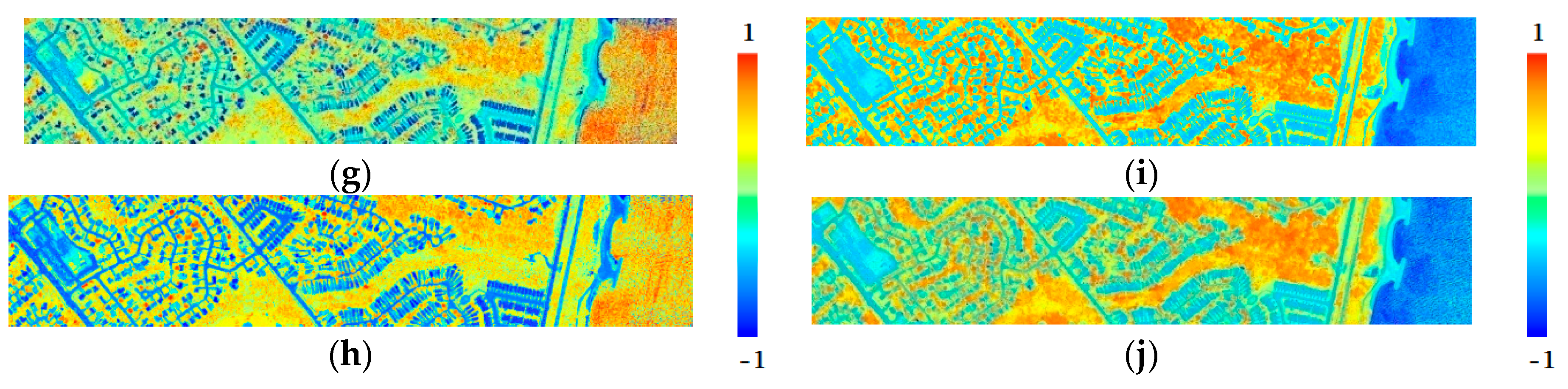
Extracted features. (a) nDSM of 532 nm channel; (b) nDSM of 1064 nm channel; (c) nDSM of 1550 nm channel; (d) curvature of 532 nm channel; (e) curvature of 1064 nm channel; (f) curvature of 1550 nm channel; (g) NDFIMIR-G image from LiDAR; (h) NDFINIR-G image from LiDAR; (i) NDVI1 image from WV-3; (j) NDVI2 image from WV-3.
Figure 4.
Extracted features. (a) nDSM of 532 nm channel; (b) nDSM of 1064 nm channel; (c) nDSM of 1550 nm channel; (d) curvature of 532 nm channel; (e) curvature of 1064 nm channel; (f) curvature of 1550 nm channel; (g) NDFIMIR-G image from LiDAR; (h) NDFINIR-G image from LiDAR; (i) NDVI1 image from WV-3; (j) NDVI2 image from WV-3.


Figure 5.
Results of Case 1. (a) Reference image; (b) the result of Case 1-1; (c) the result of Case 1-2; (d) the result of Case 1-3; (e) the result of Case 1-4.
Figure 5.
Results of Case 1. (a) Reference image; (b) the result of Case 1-1; (c) the result of Case 1-2; (d) the result of Case 1-3; (e) the result of Case 1-4.
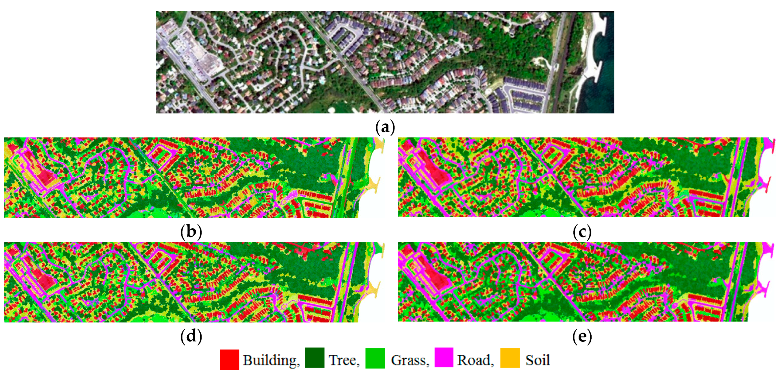
Figure 6.
Completeness and correctness for different classes in Case 1-1 to Case 1-4.

Figure 7.
Results of overall accuracies for single- and multi-wavelength LiDARs.

Figure 8.
Results of Case 2. (a) Result of Case 2-1; (b) result of Case 2-2; (c) result of Case 2-3.
Figure 8.
Results of Case 2. (a) Result of Case 2-1; (b) result of Case 2-2; (c) result of Case 2-3.

Figure 9.
Completeness and correctness for different classes in Case 2-1 to Case 2-3.

Figure 10.
Results of overall accuracies for spectral and geometrical features.

Figure 11.
Results of vegetation detection. (a) Reference image; (b) result of Case 3-1; (c) result of Case 3-2.
Figure 11.
Results of vegetation detection. (a) Reference image; (b) result of Case 3-1; (c) result of Case 3-2.

Figure 12.
Completeness and correctness for different classes in Case 3-1 to Case 3-2.
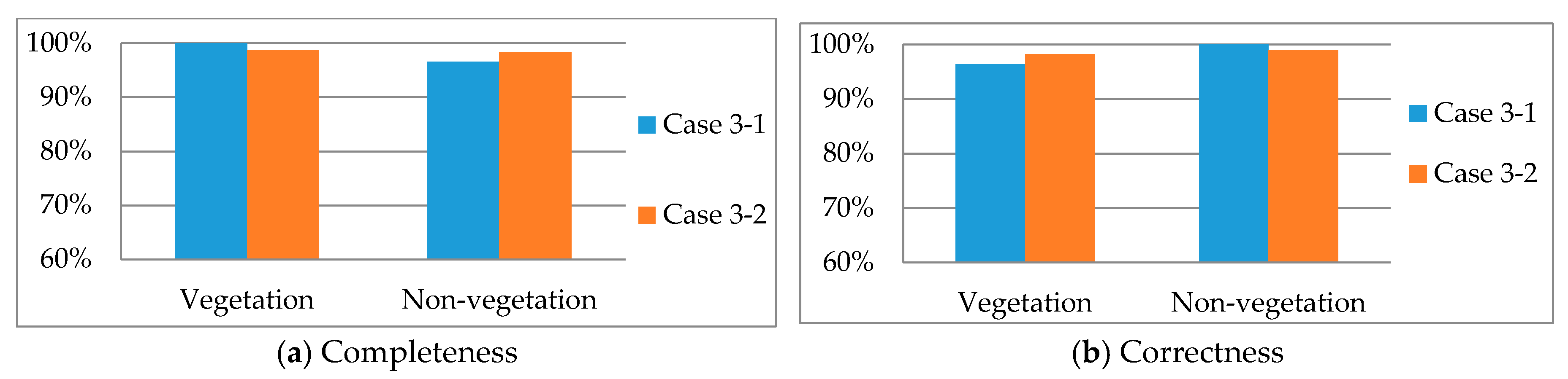
Figure 13.
Results of overall accuracies for active and passive vegetation index.

Figure 14.
R2 and RMSE between NDFIs (active) and NDVIs (passive).

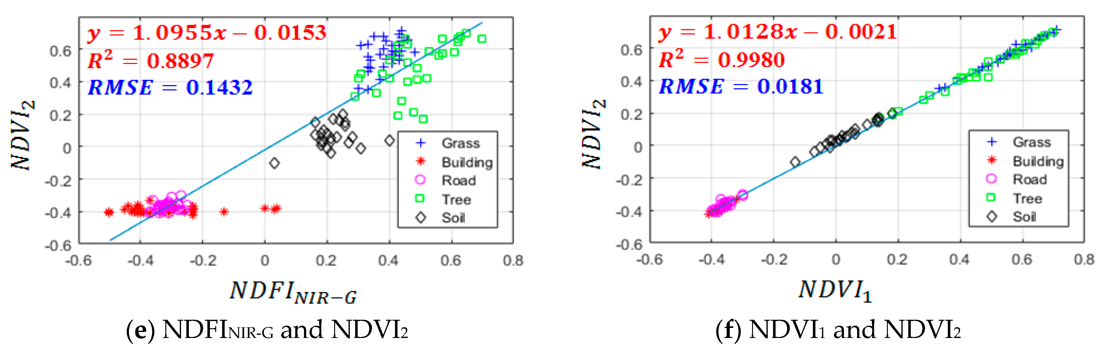
Table 1.
The specifications of Titan multi-wavelength light detection and ranging (LiDAR) system.
| Items | Channel 1 | Channel 2 | Channel 3 |
|---|---|---|---|
| Laser Wavelength (nm) | 1550 | 1064 | 532 |
| Beam divergence (mrad) | 0.35 | 0.35 | 0.7 |
| Laser classification | Class IV | Class IV | Class IV |
| Look angle (degree) | 3.5 forward | Nadir | 7.0 forward |
| Pulse repletion frequency (kHz) | 50–300 | 50–300 | 50–300 |
| Pulse energy (µJ) | 20–50 | ~15 | ~30 |
| Pulse width (ns) | ~2.7 | 3–4 | ~3.7 |
Table 2.
Point density in different land covers (Unit: points/m2).
| Density | Sum | |||
|---|---|---|---|---|
| Building | 24.8 | 23.5 | 23.2 | 71.5 |
| Grass | 32.7 | 31.9 | 29.5 | 94.1 |
| Tree | 39.6 | 46.9 | 39.2 | 125.7 |
Table 3.
Number of objects and pixels for training and test area.
| Object (Pixel) | Building | Tree | Grass | Road | Soil | Sum |
|---|---|---|---|---|---|---|
| Training | 30 (4140) | 30 (4630) | 30 (5136) | 30 (4761) | 20 (1697) | 140 (24,906) |
| Test | 30 (3212) | 30 (3337) | 30 (4166) | 30 (2967) | 20 (1284) | 140 (19,252) |
| Total | 60 (7352) | 60 (7967) | 60 (9302) | 60 (7728) | 40 (2981) | 280 (44,158) |
Table 4.
The combinations for single- and multi-wavelength LiDAR classification.
| Combinations | Features |
|---|---|
| Case 1-1 | |
| Case 1-2 | |
| Case 1-3 | |
| Case 1-4 | All features of Case 1-1, Case 1-2 and Case 1-3 |
Table 5.
Completeness and correctness for different classes in Case 1-1 to Case 1-4.
| (a) Completeness | (b) Correctness | ||||||||||
|---|---|---|---|---|---|---|---|---|---|---|---|
| Combinations | Grass | Build. | Road | Tree | Soil | Combinations | Grass | Build. | Road | Tree | Soil |
| Case 1-1 | 96.3% | 84.5% | 59.0% | 100% | 40.0% | Case 1-1 | 73.4% | 99.5% | 80.8% | 97.1% | 44.0% |
| Case 1-2 | 83.5% | 99.5% | 98.2% | 100% | 51.6% | Case 1-2 | 84.9% | 98.4% | 99.9% | 100% | 48.6% |
| Case 1-3 | 82.5% | 99.5% | 94.3% | 100% | 83.8% | Case 1-3 | 90.1% | 94.9% | 98.5% | 99.9% | 67.1% |
| Case 1-4 | 93.8% | 99.5% | 99.9% | 100% | 82.3% | Case 1-4 | 94.6% | 100% | 99.9% | 99.8% | 79.8% |
Table 6.
The combinations for spectral and geometrical features classification.
| Combinations | Features |
|---|---|
| Case 2-1 | , , , , |
| Case 2-2 | , , , , , |
| Case 2-3 | All features of Case 2-1 and Case 2-2 |
Table 7.
Completeness and correctness for different classes in Case 2-1 to Case 2-3.
| (a) Completeness | (b) Correctness | ||||||||||
|---|---|---|---|---|---|---|---|---|---|---|---|
| Combinations | Grass | Build. | Road | Tree | Soil | Combinations | Grass | Build. | Road | Tree | Soil |
| Case 2-1 | 96.6% | 81.5% | 98.2% | 96.9% | 88.3% | Case 2-1 | 98.7% | 98.0% | 84.7% | 93.1% | 86.7% |
| Case 2-2 | 18.3% | 95.0% | 62.3% | 100% | 50.7% | Case 2-2 | 34.0% | 100% | 34.3% | 99.9% | 69.3% |
| Case 2-3 | 93.8% | 99.5% | 99.9% | 100% | 94.0% | Case 2-3 | 98.1% | 100% | 99.9% | 96.9% | 87.8% |
Table 8.
The combinations for active and passive sensors classification.
| Combinations | Features |
|---|---|
| Case 3-1 | NDFIMIR-G and NDFINIR-G (from multi-wavelength LiDAR) |
| Case 3-2 | NDVI1 and NDVI2 (from WV-3 multispectral image) |
Table 9.
Completeness and correctness for different classes in Case 3-1 to Case 3-2.
| (a) Completeness | (b) Correctness | ||||
|---|---|---|---|---|---|
| Vegetation | Non-Veg. | Vegetation | Non-Veg. | ||
| Case 3-1 | 100.0% | 96.6% | Case 3-1 | 96.4% | 100.0% |
| Case 3-2 | 98.8% | 98.3% | Case 3-2 | 98.2% | 98.9% |
© 2017 by the authors. Licensee MDPI, Basel, Switzerland. This article is an open access article distributed under the terms and conditions of the Creative Commons Attribution (CC BY) license (http://creativecommons.org/licenses/by/4.0/).
Share and Cite
MDPI and ACS Style
Teo, T.-A.; Wu, H.-M. Analysis of Land Cover Classification Using Multi-Wavelength LiDAR System. Appl. Sci. 2017, 7, 663. https://doi.org/10.3390/app7070663
AMA Style
Teo T-A, Wu H-M. Analysis of Land Cover Classification Using Multi-Wavelength LiDAR System. Applied Sciences. 2017; 7(7):663. https://doi.org/10.3390/app7070663
Chicago/Turabian StyleTeo, Tee-Ann, and Hsien-Ming Wu. 2017. "Analysis of Land Cover Classification Using Multi-Wavelength LiDAR System" Applied Sciences 7, no. 7: 663. https://doi.org/10.3390/app7070663
Note that from the first issue of 2016, this journal uses article numbers instead of page numbers. See further details here.