
Adaptive Neuro-Fuzzy Inference System Model Based on the Width and Depth of the Defect in an Eddy Current Signal


1
Faculty of Electrical and Electronics, University Malaysia Pahang, Pekan 26600, Malaysia
2
Faculty of Engineering Technology, University Malaysia Pahang, Kuantan 26300, Malaysia, [email protected]
3
Faculty of Electrical & Automation Engineering Technology, TATI University College, Kemaman 26000, Malaysia
*
Author to whom correspondence should be addressed.
Appl. Sci. 2017, 7(7), 668; https://doi.org/10.3390/app7070668
Submission received: 17 March 2017
/
Revised: 24 June 2017
/
Accepted: 25 June 2017
/
Published: 29 June 2017
Abstract
:Non-destructive evaluation (NDE) plays an important role in many industrial fields, such as detecting cracking in steam generator tubing in nuclear power plants and aircraft. This paper investigates on the effect of the depth of the defect, width of the defect, and the type of the material on the eddy current signal which is modeled by an adaptive neuro-fuzzy inference system (ANFIS). A total of 60 samples of artificial defects are located 20 mm parallel to the length of the block in each of the three types of material. A weld probe was used to inspect the block. The ANFIS model has three neurons in the input layer and one neuron in the output layer as the eddy current signal. The used design of experiments (DOE) software indicates that the model equations, which contain only linear and two-factor interaction terms, were developed to predict the percentage signal. This signal was validated through the use of the unseen data. The predicted results on the depth and width of defect significantly influenced the percentage of the signal (p < 0.0001) at the 95% confidence level. The ANFIS model proves that the deviation of the eddy current testing measurement was influenced by the width and depth of the defect less than the conductivity of the materials.
1. Introduction
Non-destructive testing and evaluation is the process of assessing the structural integrity of a material or component without causing any physical damage to the test object [1]. Eddy current testing is an effective method to detect fatigue cracks and corrosion in conductive materials because it is cheap and can monitor subsurface defects or defects under insulating coatings without touching the surface of a specimen [2,3].
Many studies investigated the effect of different parameters on eddy current signal. Material permeability and strength of magnetic induction are influenced by the type of material [4]. Thus, more secondary electromagnetic waves are produced in ferrous metals than in non-ferrous metals. Therefore, permeability significantly influences the eddy current defect signal. Crack orientation strongly influences the output of the eddy current probe. Cracks must interrupt the surface eddy current flow to be detected. Defects parallel to the current path will not cause any significant interruption and may not be detected [5,6,7,8]. The response of the pickup coil or receiver coil to an eddy current depends on the conductivity and permeability of the test material and the frequency selected [9].
Artificial intelligence was used in many types of research in eddy current testing. In [10] Postolache proposed a neural network algorithm for fast classification of the aluminum plate defects, such as cracks and holes. Moreover, the discrete wavelet transform allied with an artificial neural network (ANN) was used in [11] to estimate the depth of defect based on eddy current testing ECT data. Morabito and Versaci introduced a fuzzy neural approach to localize holes in conducting plates. However, the limitation is that fuzzy inference systems are effective with a few number of inputs [12]. In 2016 an ANN with the statistical technique of principal component analysis PCA was applied to steam generator data in simultaneous measurement by using PEC. Combining PCA and ANN improves the sensitivity of pulsed eddy current PEC [13].
The eddy current testing was investigated and, statistically, the optimized condition was achieved through response surface methodology (RSM) using central composite design. An adaptive neuro-fuzzy inference system (ANFIS) model was utilized to compare with RSM. The materials of the artificial defect block are mild steel, brass, and copper with dimensions of 420 × 30 × 10 mm. The depth of the defect is between 1 and 2.5 mm from the surface of the artificial defect block, whereas the width of a defect is located between 0.2 and 1 mm. The ANFIS model is used to predict the future behavior of processes, as well as the evaluation of the statistical significance of the effects of the process effects on the desired response.
2. Materials and Methods
2.1. Materials
Three different materials were used to fabricate calibration blocks (copper, brass, and mild steel). The material conductivities of copper, brass, and mild steel were 99.75%, 23.65%, and 8.48%, respectively, based on International Annealed Copper Standard. The materials were used as calibration blocks with dimensions of 260 mm (length) × 30 mm (width) × 10 mm (height). A total of 20 slots of artificial defects with different depths were produced by performing surface grinding, milling process and electrical discharge machining. AutoCAD (Autodesk, San Rafael, CA, USA) 2004 design software was used to design the artificial defect slots.
2.2. Inspection the Calibration Blocks Using a Weld Probe
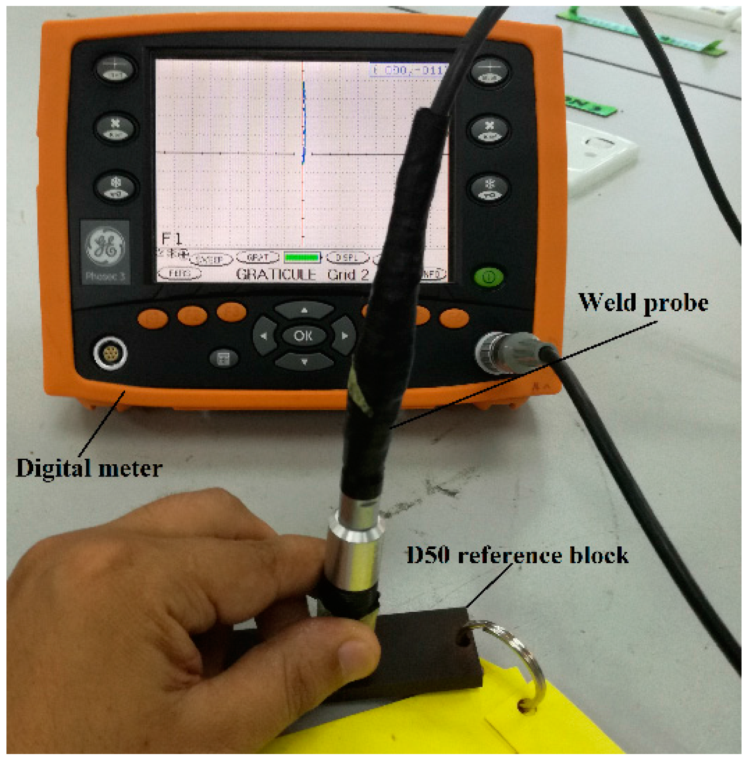
A weld (differential) probe was used to inspect the materials. The locator menu was first adjusted to the appropriate settings, as shown in Table 1. The positive and negative index points were indicated on the probe by maximizing the 1 mm notch in the D50 reference block, which is used to calibrate the weld probe, as shown in Figure 1.
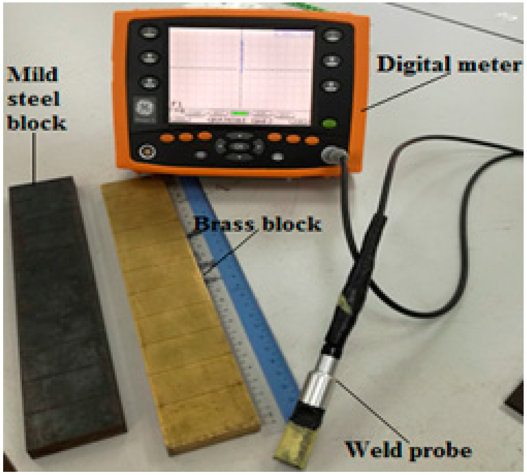
Figure 2 shows the images of a commercial ECT system and test specimens. The accurate gain, frequency, and velocity were considered to inspect all materials. All results were used to compare the defect signal of the width on different block materials and to measure the variations of the eddy current between the brass block, copper block, and mild steel block.
3. Proposed ANFIS Model
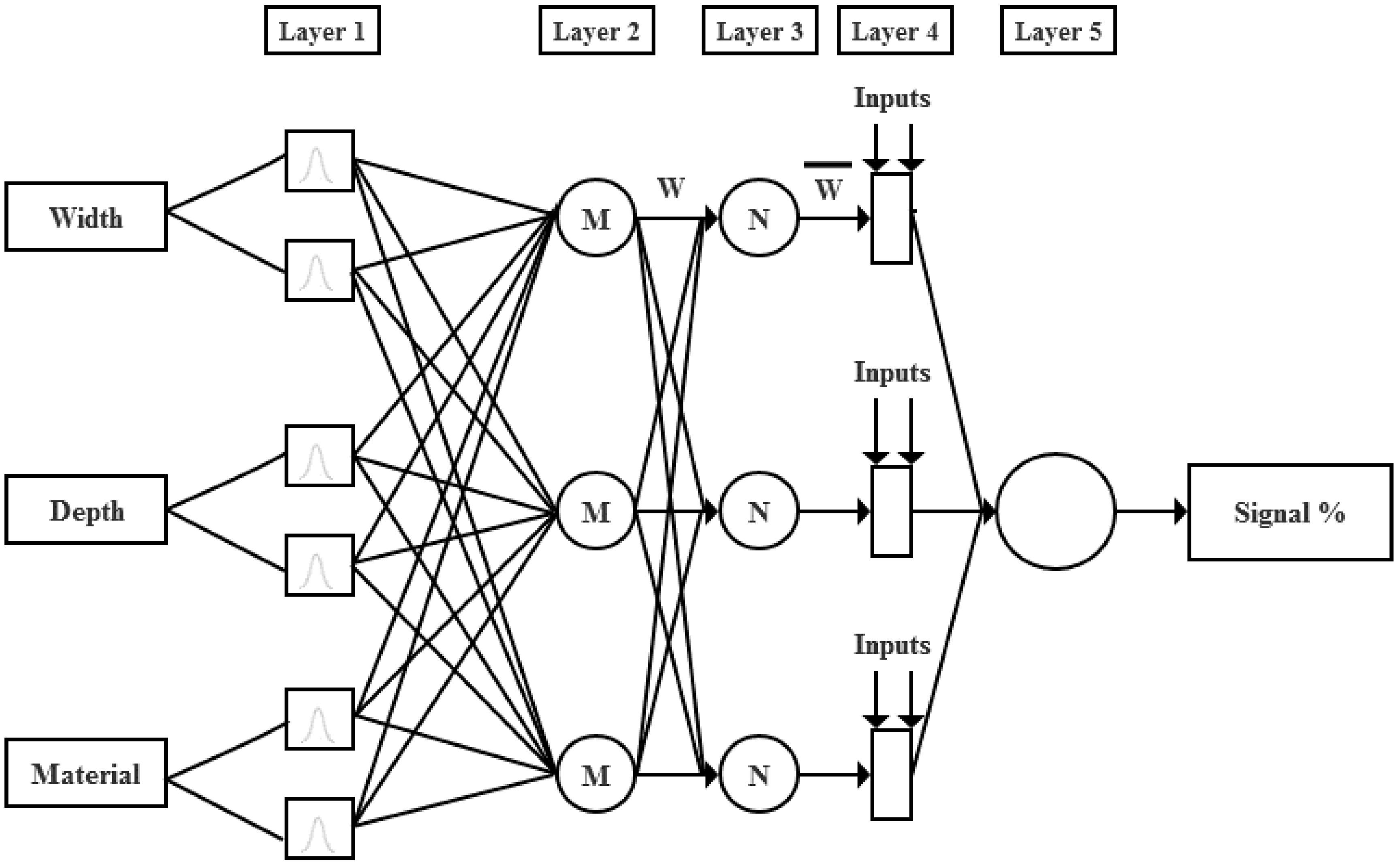
The MATLAB Neural Network Toolbox R2013a (MathWorks, Natick, MA, USA) was used to train and optimize ANNs. ANFIS is an adaptive network which allows the implementation of a neural network topology with fuzzy logic [14,15]. An ANFIS study compiles these two methods and utilizes the characteristics of both methods. In addition, ANFIS gathers the neural network and fuzzy logic and can address nonlinear and complex problems [16]. ANFIS is a class of adaptive multilayer feed-forward networks, which are functionally equivalent to a fuzzy inference system. The Takagi–Sugeno fuzzy inference system, which contains a five-membership and simple schematic of the proposed ANFIS model, is shown in Figure 3. The proposed model and all tests were implemented using MATLAB. The error function used is a function of the logistic sigmoid and standard total of squared error function.
The model inputs include the type of material, the width of the crack, and the depth of the crack. The model outputs include the percentage of the signal. The training data were collected experimentally and normalized to obtain the values. The formula used is as follows:
Low + (High − Low) × Actual value − Minimum/Maximum − Minimum
Low is the minimum normalized data value, which is equal to 0.1, and minimum is the minimum data value. High is the maximum normalized data value, which is equal to 0.9, and the maximum is the maximum data value [17].
4. Experimental Designs
The central composite design (CCD) was employed in the optimization study of the eddy current testing. The depth of defect, width of defect, and type of material were the independent variables (process factors) selected to optimize the percentage of the signal (response). Furthermore, RSM is used to generate the mathematical equation for the actual functional relationship between the dependent parameter (y) and the independent parameters. The first-order model is considered for linear function models of the independent parameters:
If the system has curvature, then the second-order model should be considered:
where y is the response (dependent variable, i.e., the percentage of the signal), b0 is the constant regression coefficient, bi and bii are the linear and quadratic regression coefficients, respectively, and bij is the regression coefficients of the two-factor interactions (i, j, = 1,2,3). xi, xj are the process factors (independent variables, i.e., type of material, depth of defect and width of defect). The fit of the model equation was evaluated by ANOVA, revealing the statistically-significant process factors with the confidence level of 95% (p-value < 0.05). The developed second-order polynomial equation was then modified by eliminating the insignificant terms. The CCD consisted of 60 experiments including five centre points, to identify the error. The design was executed with Design Expert software.
5. Results and Discussion
5.1. Inspection Results for Mild Steel Blocks
The effect of the depth of the defect and the width of the defect with mild steel on the eddy current testing signal could be detected by the weld probe. The inspection was conducted by using a frequency of 100 kHz. The amplitude was set to 100% FSH, and the gain was set to 50 dB (approximate). Table 2 shows the signal of the eddy current testing measurements for mild steel with different depths and widths.
5.2. The DOE Analysis
Design Expert 7 software was used to investigate the impact of the simulated runs on the responses. Numerical data revealed that the percentage of the signal is varied between 0.38 and 1. Table 3 shows that the value of total determination R2 is 0.8808% (close to 1), which indicates that the quadratic model reasonably fits the numerical data and can represent signal percentage in terms of the independent parameters [18]. The significance of each parameter was determined (p < 0.05) using the p-value.
Table 3 shows that the analysis of variance (ANOVA) of the independent parameters, depth of the defect, and width of the defect were significant (p < 0.05). Additionally, the type of material, the interaction impact of depth of defect with the type of material, width of the defect with the type of material, depth of the defect with width of the defect, quadratic terms of the depth of the defect, and quadratic terms of the width of the defect were not significant, given that the p-values are 0.0004, 0.6257, 0.0254, 0.0020, 0.0002, and 0.3040, respectively. Thus, non-significant terms were eliminated, and the optimization process was repeated until all terms become significant.
The implementation of RSM provides the following regression equation, which can be considered an empirical relationship between the percentage of the signal and the independent parameters.
where y is the percentage of the signal, X1 is the type of material, X2 is the depth of the defect, and X3 is the width of the defect.
y = +0.29064 − 8.69189 × 10⁻³ × X1 + 0.24640 × X2 + 0.18250 × X3 + 7.45897 × 10⁻⁵ × X12
5.2.1. The Effect of the Depth of the Defect and Width of the Defect on the Response
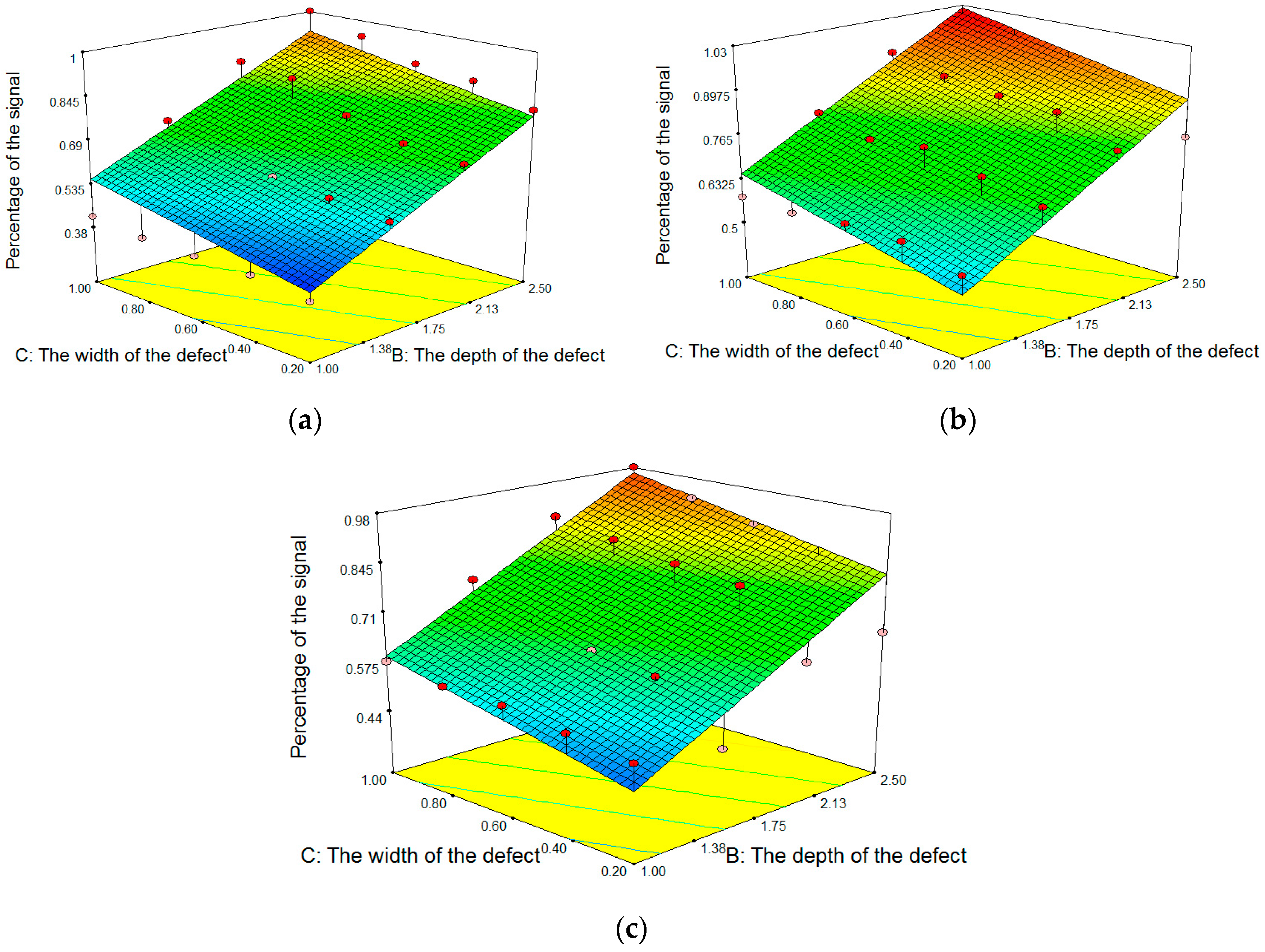
Figure 4 shows the response surface 3D plots with contour plots on their bases for the percentage of the signal as a function of the depth of the defect and width of the defect. Figure 4a shows the results for brass, and Figure 4b shows the results for mild steel. Figure 4c shows the results for copper. In general, these plots are useful to visualize the effects of the process factors and their interactions on the percentage of the signal and the optimal process conditions. The designs provided the results, where the percentage of the signal increased with the increase in depth and width of the defect and conductivity of the material. Figure 4a shows that, for brass, the influence of the depth of the defect on the percentage of the signal was insignificant when the width of the defect was narrow. The influence of the depth of the defect on the percentage of the signal was significant when the width was increased.
With mild steel, the increase in the percentage of the signal was evident, as shown in Figure 4b. The interactive effect of the size of the depth and size of the width on the percentage of signal was similar to that of brass, except that the obtained percentage of a signal was lower with brass. This result was explained by the negative effect of the type of material on the percentage of the signal formation. With the copper material, the percentage of signal continued to increase, as shown in Figure 4c. The effect of the depth of defect on the percentage of the signal was more significant at wide than at narrow defect widths.
5.2.2. The Effect of Defect Width and the Type of Material on the Response
Figure 5 shows the effect of the defect width and type of material on the signal output at a defect depth of 2.5 mm. The material type and defect width show significant effect on output signal, and the interaction of both shows an insignificant effect.
5.2.3. The Effect of Defect Depth and the Type of Material on the Response
Figure 6 shows the effect of the defect depth and the type of the material on the signal output with a defect width of 1 mm. The material type and defect depth show a significant effect on the output signal, and the interaction of both shows an insignificant effect.
To benchmark the accuracy of the present RSM models, Figure 7 compared the predicted values of the percentage of the signal, which were obtained using the regression models with the experimental values. Figure 7 evidently shows good agreement between the experimental results of the percentage of the signal and the predicted values using the developed regression equations.
5.3. ANFIS Simulation Results
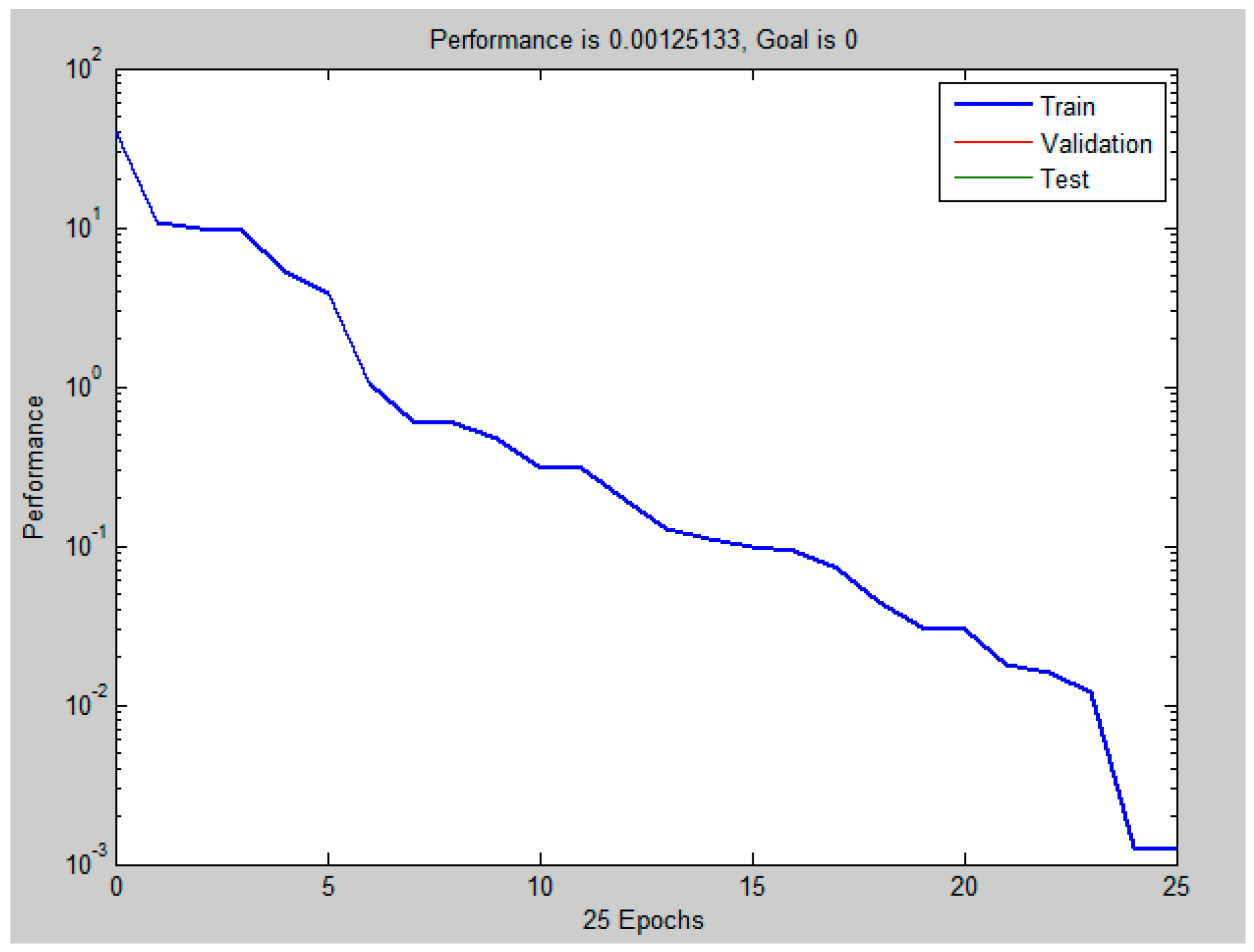
Sixty experimental data records were used to verify the performances of the ANFIS models. To improve the ANFIS model, approximately 75% of the data were used for training and the remainder for testing the performance. In Table 4, the training and testing experimental data are specified at the different run numbers. Figure 8 shows that the training optimized structure was selected as ANFIS, based on the percentage error minimum at 25 epochs.
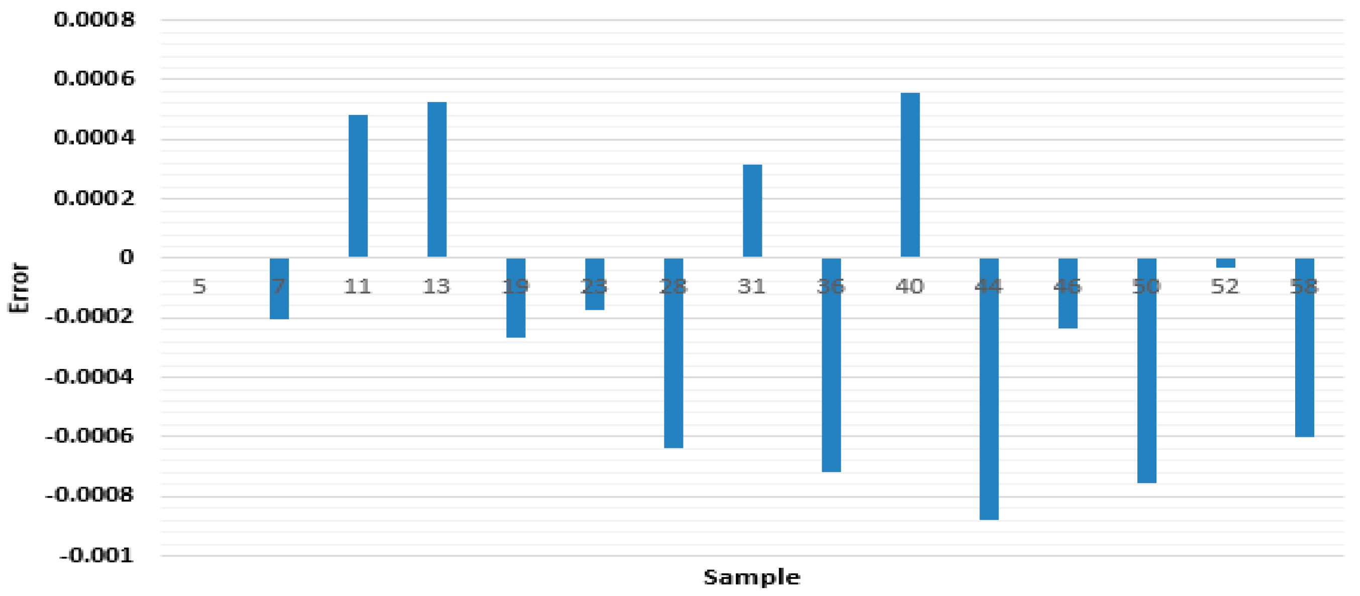
The relative error results of ANFIS model are shown in Figure 9 for training data, where the percentage error (ER) for the input test variable and the average error (AER) are estimated as follows:
where ER%, YEX, and YPre are the error percentage values, experimental test data, and ANFIS predicted values, respectively.
The ANFIS models for training and testing data are shown in Figure 10. The numerical and predicted values of the average percentage of the signal using the ANFIS model are in good agreement with the R-squared value of 0.9983. Table 5 shows that the maximum percentage error and average percentage error were approximately 0.000998 and 0.000493, respectively.
6. Conclusions
In short, the processing variables of eddy current testing have been experimentally studied in detail. Based on the RSM model, the most effective factor on the percentage of the signal is the depth of the defect in the present study. The ANFIS model is developed to predicate the percentage signal of the eddy current testing measurements. The ANFIS models can be used effectively to estimate the characteristics of defects. The study results can be summarized as follows:
- For the percentage signal, the maximum error for trained and tested values is 0.023%, and the average error is 0.000493 in the ANFIS model.
- The prediction of the averaged percentage signal with the ANFIS models is in good agreement with the experimental result; it also has a smaller error.
The results prove that material conductivity and the size of cracks directly affect the eddy current signal.
Acknowledgments
This work was supported by Malaysia Pahang under project vote RDU1403116.
Author Contributions
Moneer A. Faraj and Fahmi Samsuri designed and arranged the structure of the article; Kharudin Ali and Damhuji Rifai performed the experiments; Ahmed N. Abdalla analyzed the data preview in the previous work in this field; and Moneer A. Faraj and Ahmed N. Abdalla wrote the paper.
Conflicts of Interest
The authors declare no conflict of interest regarding the publication of this paper.
References
- Rifai, D.; Abdalla, A.N.; Ali, K.; Razali, R. Giant Magnetoresistance Sensors: A Review on Structures and Non-Destructive Eddy Current Testing Applications. Sensors 2016, 16, 298. [Google Scholar] [CrossRef] [PubMed]
- Ali, K.; Abdalla, A.N.; Rifai, D.; Faraj, M. A Review on System Development in Eddy Current Testing and Technique for Defect Classification and Characterization. IET Circuits Devices Syst. 2017. [Google Scholar] [CrossRef]
- Garcia-Martin, J.; Gomez-Gil, J.; Vazquez-Sanchez, E. Non-destructive techniques based on eddy current testing. Sensors (Basel) 2011, 11, 2525–2565. [Google Scholar] [CrossRef] [PubMed]
- Faraj, M.A.; Abdalla, A.N.; Samsuri, F.B.; Rifai, D.; Ali, K. Investigate of the Effect of Width Defect on Eddy Current Testing Signals under Different Materials. Indian J. Sci. Technol. 2017, 10. [Google Scholar] [CrossRef]
- Lee, K.H.; Baek, M.K.; Park, I.H. Estimation of deep defect in ferromagnetic material by low frequency eddy current method. IEEE Trans. Magn. 2012, 48, 3965–3968. [Google Scholar] [CrossRef]
- Biju, N.; Ganesan, N.; Krishnamurthy, C.; Balasubramaniam, K. Optimum frequency variations with coil geometry and defects in tone burst eddy current thermography (TBET). Insight-Non-Destr. Test. Cond. Monit. 2013, 55, 504–509. [Google Scholar] [CrossRef]
- Rosado, L.S.; Janeiro, F.M.; Ramos, P.M.; Piedade, M. Defect characterization with eddy current testing using nonlinear-regression feature extraction and artificial neural networks. IEEE Trans. Instrum. Meas. 2013, 62, 1207–1214. [Google Scholar] [CrossRef]
- Rifai, D.; Abdalla, A.N.; Khamsah, N.; Aizat, M.; Fadzli, M. Subsurface Defects Evaluation using Eddy Current Testing. Indian J. Sci. Technol. 2016, 9. [Google Scholar] [CrossRef]
- Sasayama, T.; Ishida, T.; Matsuo, M.; Enpuku, K. Thickness Measurement of an Iron Plate Using Low-Frequency Eddy Current Testing With an HTS Coil. IEEE Trans. Appl. Superconduct. 2016, 26, 1–5. [Google Scholar] [CrossRef]
- Postolache, O.; Ramos, H.G.; Ribeiro, A.L. Characterization of defects in aluminum plates using GMR probes and neural network signal processing. In Proceedings of the XVI-IMEKO TC4 Symposium, Florence, Italy, 22–24 September 2008. [Google Scholar]
- Bodruzzaman, M.; Zein-Sabatto, S. Estimation of micro-crack lengths using eddy current C-scan images and neural-wavelet transform. In Proceedings of the Southeastcon 2008 IEEE, Huntsville, AL, USA, 3–6 April 2008; pp. 551–556. [Google Scholar]
- Morabito, E.; Versaci, M. A fuzzy neural approach to localizing holes in conducting plates. IEEE Trans. Magn. 2001, 37, 3534–3537. [Google Scholar] [CrossRef]
- Buck, J.A.; Underhill, P.R.; Morelli, J.E.; Krause, T.W. Simultaneous multiparameter measurement in pulsed eddy current steam generator data using artificial neural networks. IEEE Trans. Instrum. Meas. 2016, 65, 672–679. [Google Scholar] [CrossRef]
- Jang, J.S.; Sun, C.T. Neuro-Fuzzy Modeling and Control. Proc. IEEE 1995, 83, 378–406. [Google Scholar] [CrossRef]
- Jang, J.S.R.; Sun, C.T.; Mizutani, E. Neuro-Fuzzy and Soft Computing, a Computational Approach to Learning and Machine Intelligence; Prentice Hall, Inc: Upper Saddle River, NJ, USA, 1997. [Google Scholar]
- Bunke, H.; Kandel, A. Neuro-Fuzzy Pattern Recognition; World Scientific Publishing Company: Singapore, 2000; Volume 41. [Google Scholar]
- Fausett, L.V. Fundamentals of Neural Networks; Prentice-Hall, Inc: Upper Saddle River, NJ, USA, 1994. [Google Scholar]
- Firatligil-Durmus, E.; Evranuz, O. Response surface methodology for protein extraction optimization of red pepper seed (Capsicum frutescens). LWT-Food Sci. Technol. 2010, 43, 226–231. [Google Scholar] [CrossRef]
Figure 1.
Calibrated weld probe by using a calibration block.

Figure 2.
Images of commercial ECT system and test specimens.

Figure 3.
Adaptive neuro-fuzzy inference system (ANFIS) model.

Figure 4.
3D graphic surface optimization of the percentage of the signal as influenced by the width and the depth of the defect of (a) brass material; (b) mild steel material; and (c) copper material.
Figure 4.
3D graphic surface optimization of the percentage of the signal as influenced by the width and the depth of the defect of (a) brass material; (b) mild steel material; and (c) copper material.

Figure 5.
3D graphic surface optimization of percentage of the signal as influenced by the width of the defect and the type of material with the depth of the defect of 2.5 mm.
Figure 5.
3D graphic surface optimization of percentage of the signal as influenced by the width of the defect and the type of material with the depth of the defect of 2.5 mm.
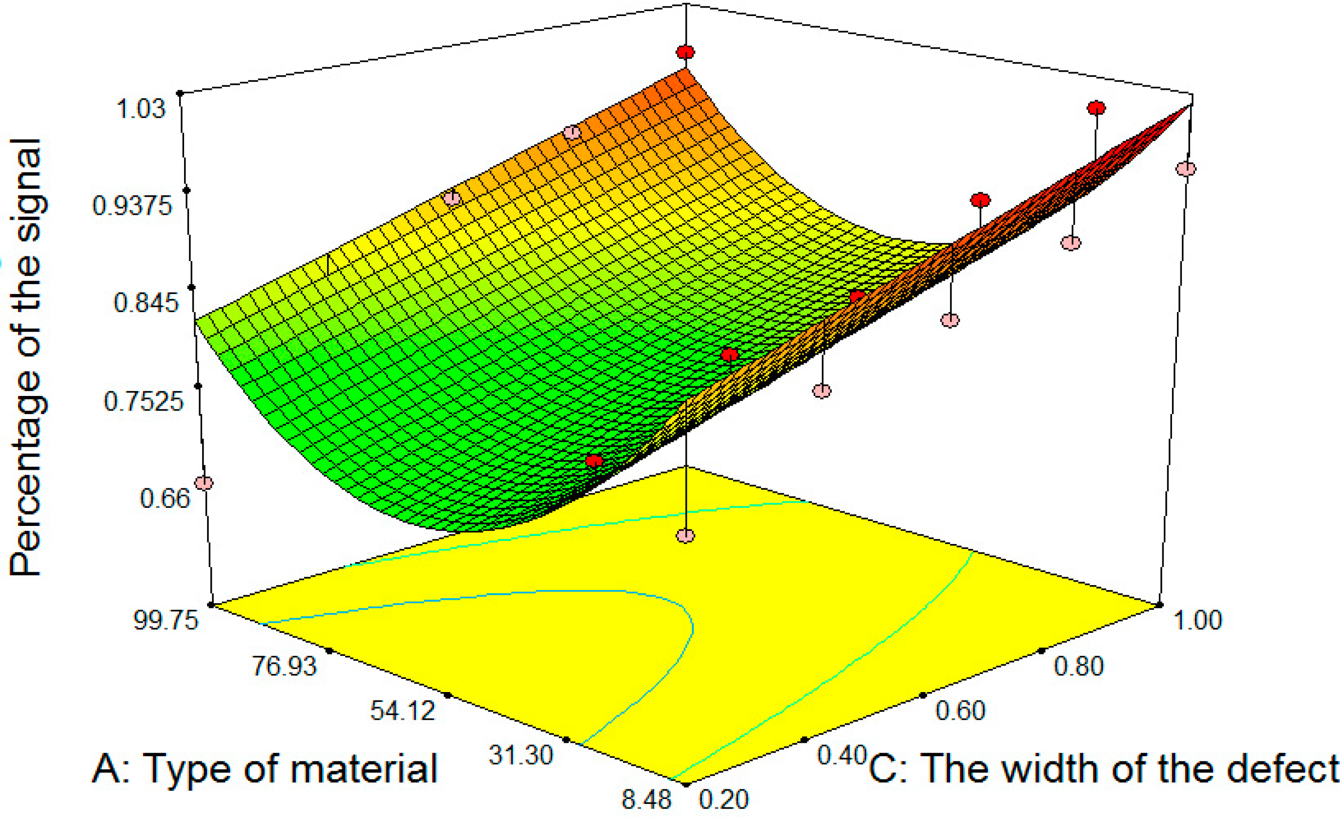
Figure 6.
3D graphic surface optimization of percentage of the signal as influenced by the depth of the defect and the type of material with a width of the defect of 1 mm.
Figure 6.
3D graphic surface optimization of percentage of the signal as influenced by the depth of the defect and the type of material with a width of the defect of 1 mm.
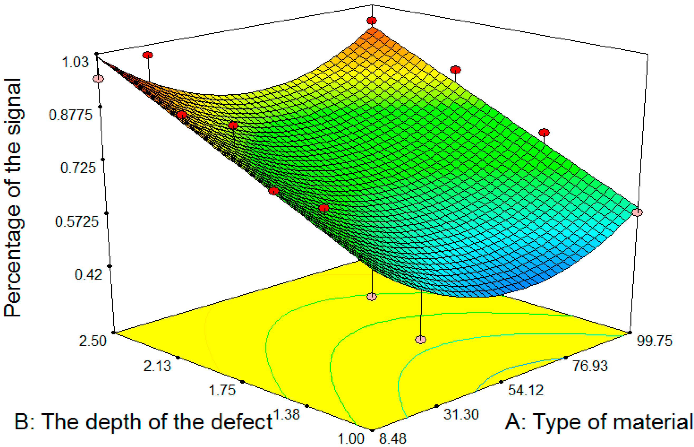
Figure 7.
Predicted and actual values of the signal percentage.
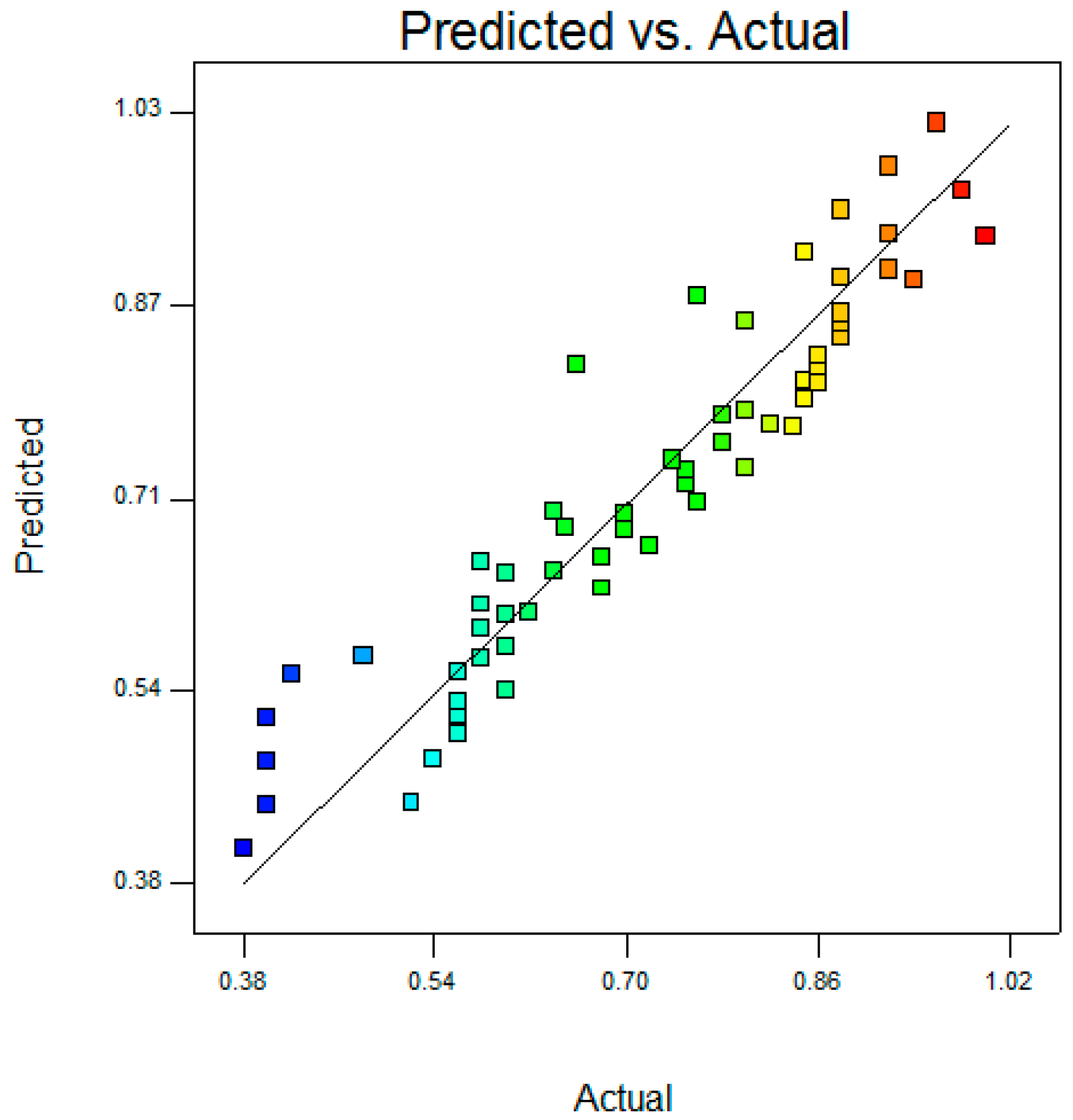
Figure 8.
ANFIS training.

Figure 9.
Percentage error of ANFIS models for training data.
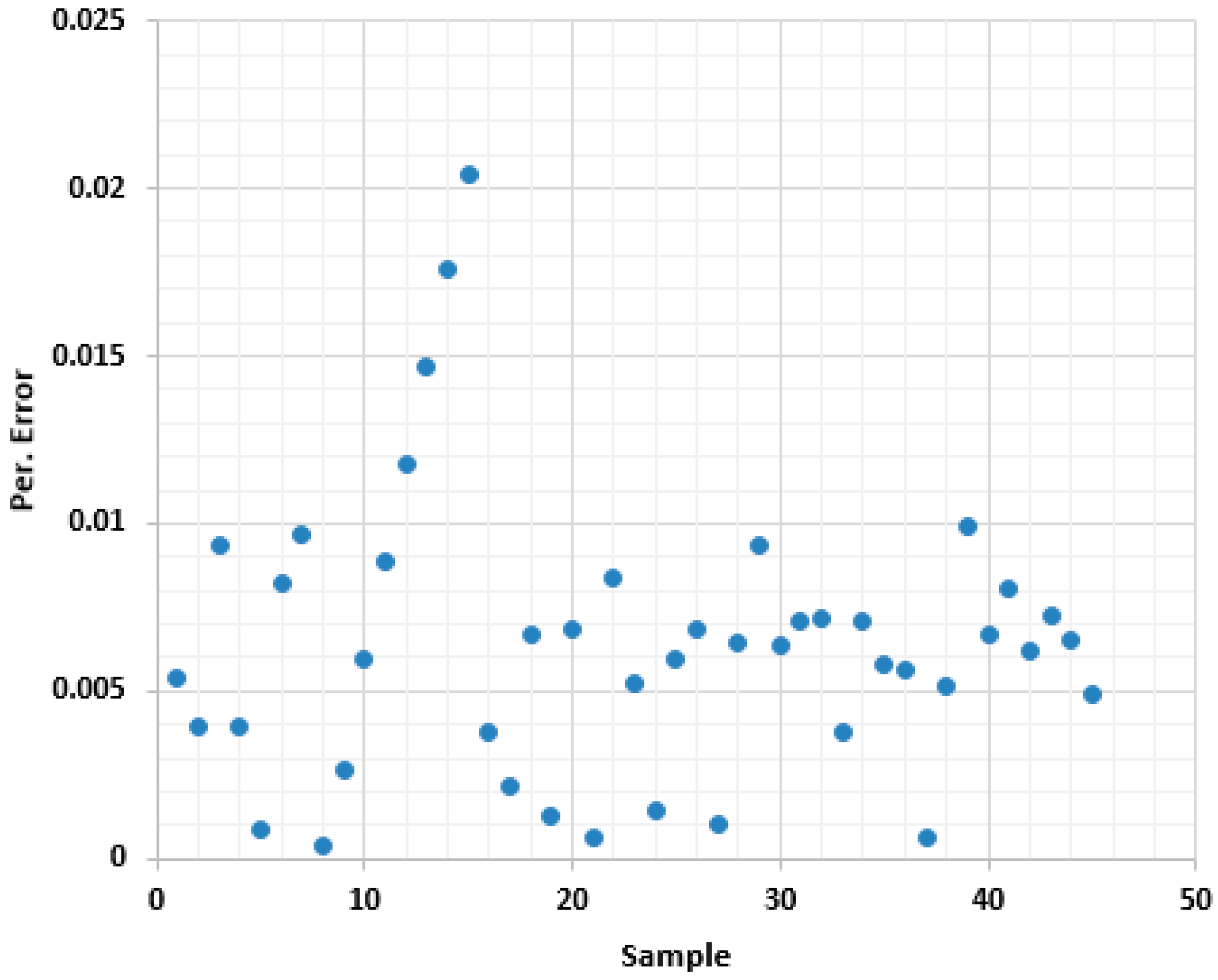
Figure 10.
Error between experimental and ANFIS predicted values for each sample.


Table 1.
Weld probe settings.
| Frequency | Gain | Probe | Persistence | Phase | Spot X/Y |
|---|---|---|---|---|---|
| 100 KHz | 50 dB (approx.) | Bridge | Permanent | Set to 12 o’clock 100% FSH | Centre of the screen |
Table 2.
Results for mild steel.
| The Depth of Defect (mm) | The Width of Defect (mm) | Signal Display | Percentage Signal |
|---|---|---|---|
| 1 | 0.2 |  | 56% |
| 1.5 | 0.4 |  | 72% |
| 2 | 0.6 |  | 86% |
| 2.5 | 0.8 |  | 92% |
| 1.5 | 1 |  | 58% |
Table 3.
ANOVA for response surface quadratic model of the signal percentage.
| Source | Sum of Square | Df | Mean Square | F Value | p-Value Prob > F |
|---|---|---|---|---|---|
| Model | 1.39 | 4 | 0.35 | 101.58 | <0.0001 |
| A-material | 0.032 | 1 | 0.032 | 9.33 | 0.0035 |
| B-depth | 1.14 | 1 | 1.14 | 332.66 | <0.0001 |
| C-width | 0.16 | 1 | 0.16 | 46.72 | <0.0001 |
| A2 | 0.060 | 1 | 0.086 | 25.15 | <0.0001 |
| Residual | 0.19 | 55 | 3.422 × 10⁻³ | ||
| Cor Total | 1.58 | 59 |
Table 4.
Training and experimental testing data.
| Experiment Runs | Type of Material | Depth of Crack | Width of Crack | Percentage of Signal |
|---|---|---|---|---|
| Training data | ||||
| 1 | 1 | 1 | 0.2 | 0.56 |
| 2 | 1 | 1 | 0.4 | 0.6 |
| 3 | 1 | 1 | 0.6 | 0.6 |
| 4 | 1 | 1 | 0.8 | 0.58 |
| 6 | 1 | 1.5 | 0.2 | 0.68 |
| 8 | 1 | 1.5 | 0.6 | 0.76 |
| 9 | 1 | 1.5 | 0.8 | 0.74 |
| 10 | 1 | 1.5 | 1 | 0.78 |
| 12 | 1 | 2 | 0.4 | 0.85 |
| 14 | 1 | 2 | 0.8 | 0.88 |
| 15 | 1 | 2 | 1 | 0.92 |
| 16 | 1 | 2.5 | 0.2 | 0.76 |
| 17 | 1 | 2.5 | 0.4 | 0.85 |
| 18 | 1 | 2.5 | 0.6 | 0.88 |
| 20 | 1 | 2.5 | 1 | 0.96 |
| 21 | 2 | 1 | 0.2 | 0.38 |
| 22 | 2 | 1 | 0.4 | 0.4 |
| 24 | 2 | 1 | 0.8 | 0.4 |
| 25 | 2 | 1 | 1 | 0.42 |
| 26 | 2 | 1.5 | 0.2 | 0.56 |
| 27 | 2 | 1.5 | 0.4 | 0.58 |
| 29 | 2 | 1.5 | 0.6 | 0.6 |
| 30 | 2 | 1.5 | 1 | 0.7 |
| 32 | 2 | 2 | 0.4 | 0.7 |
| 33 | 2 | 2 | 0.6 | 0.75 |
| 34 | 2 | 2 | 0.8 | 0.84 |
| 35 | 2 | 2 | 1 | 0.86 |
| 37 | 2 | 2.5 | 0.4 | 0.86 |
| 38 | 2 | 2.5 | 0.6 | 0.88 |
| 39 | 2 | 2.5 | 0.8 | 0.94 |
| 41 | 3 | 1 | 0.2 | 0.52 |
| 42 | 3 | 1 | 0.4 | 0.54 |
| 43 | 3 | 1 | 0.6 | 0.56 |
| 45 | 3 | 1 | 1 | 0.58 |
| 47 | 3 | 1.5 | 0.4 | 0.62 |
| 48 | 3 | 1.5 | 0.6 | 0.64 |
| 49 | 3 | 1.5 | 0.8 | 0.65 |
| 51 | 3 | 2 | 0.2 | 0.64 |
| 53 | 3 | 2 | 0.6 | 0.82 |
| 54 | 3 | 2 | 0.8 | 0.85 |
| 55 | 3 | 2 | 1 | 0.88 |
| 56 | 3 | 2.5 | 0.2 | 0.66 |
| 57 | 3 | 2.5 | 0.4 | 0.8 |
| 59 | 3 | 2.5 | 0.8 | 0.92 |
| 60 | 3 | 2.5 | 1 | 0.98 |
| Testing data | ||||
| 5 | 1 | 1 | 1 | 0.58 |
| 7 | 1 | 1.5 | 0.4 | 0.72 |
| 11 | 1 | 2 | 0.2 | 0.78 |
| 13 | 1 | 2 | 0.6 | 0.86 |
| 19 | 1 | 2.5 | 0.8 | 0.92 |
| 23 | 2 | 1 | 0.6 | 0.4 |
| 28 | 2 | 1.5 | 0.8 | 0.6 |
| 31 | 2 | 2 | 0.2 | 0.68 |
| 36 | 2 | 2.5 | 0.2 | 0.8 |
| 40 | 2 | 2.5 | 1 | 1 |
| 44 | 3 | 1 | 0.8 | 0.56 |
| 46 | 3 | 1.5 | 0.2 | 0.48 |
| 50 | 3 | 1.5 | 1 | 0.75 |
| 52 | 3 | 2 | 0.4 | 0.8 |
| 58 | 3 | 2.5 | 0.6 | 0.88 |
Table 5.
Comparison between the numerical result and ANFIS models for testing data.
| Exp. Run | Signal % | ANFIS | ER% |
|---|---|---|---|
| 5 | 0.58 | 0.57900165 | −0.001 |
| 7 | 0.72 | 0.71979543 | −0.0002 |
| 11 | 0.78 | 0.78048298 | 0.000483 |
| 13 | 0.86 | 0.86052741 | 0.000527 |
| 19 | 0.92 | 0.91973257 | −0.00027 |
| 23 | 0.4 | 0.39982569 | −0.00017 |
| 28 | 0.6 | 0.59936003 | −0.00064 |
| 31 | 0.68 | 0.68031255 | 0.000313 |
| 36 | 0.8 | 0.79928399 | −0.00072 |
| 40 | 1 | 1.0005583 | 0.000558 |
| 44 | 0.56 | 0.5591191 | −0.00088 |
| 46 | 0.48 | 0.47976182 | −0.00024 |
| 50 | 0.75 | 0.74924405 | −0.00076 |
| 52 | 0.8 | 0.79996763 | −3.2 × 10⁻⁵ |
| 58 | 0.88 | 0.87939948 | −0.0006 |
| Maximum | 0.000998 | ||
| ABS Average | 0.000493 |
© 2017 by the authors. Licensee MDPI, Basel, Switzerland. This article is an open access article distributed under the terms and conditions of the Creative Commons Attribution (CC BY) license (http://creativecommons.org/licenses/by/4.0/).
Share and Cite
MDPI and ACS Style
Faraj, M.A.; Samsuri, F.; Abdalla, A.N.; Rifai, D.; Ali, K. Adaptive Neuro-Fuzzy Inference System Model Based on the Width and Depth of the Defect in an Eddy Current Signal. Appl. Sci. 2017, 7, 668. https://doi.org/10.3390/app7070668
AMA Style
Faraj MA, Samsuri F, Abdalla AN, Rifai D, Ali K. Adaptive Neuro-Fuzzy Inference System Model Based on the Width and Depth of the Defect in an Eddy Current Signal. Applied Sciences. 2017; 7(7):668. https://doi.org/10.3390/app7070668
Chicago/Turabian StyleFaraj, Moneer A, Fahmi Samsuri, Ahmed N. Abdalla, Damhuji Rifai, and Kharudin Ali. 2017. "Adaptive Neuro-Fuzzy Inference System Model Based on the Width and Depth of the Defect in an Eddy Current Signal" Applied Sciences 7, no. 7: 668. https://doi.org/10.3390/app7070668
Note that from the first issue of 2016, this journal uses article numbers instead of page numbers. See further details here.