
Numerical Calculation of the Performance of a Thermoacoustic System with Engine and Cooler Stacks in a Looped Tube

1
The graduate school of Bio-Applications and Systems Engineering, Tokyo University of Agriculture and Technology, Tokyo 184-8588, Japan, [email protected]
2
Department of Physics education, Faculty of Mathematics, Natural Sciences and Information Technology Education, The University of PGRI Semarang, Jl. Sidodadi Timur Nomor 24-Dr. Cipto, Karangtempel, Semarang, Jawa Tengah 50232, Indonesia
*
Author to whom correspondence should be addressed.
Appl. Sci. 2017, 7(7), 672; https://doi.org/10.3390/app7070672
Submission received: 3 February 2017
/
Revised: 16 June 2017
/
Accepted: 27 June 2017
/
Published: 30 June 2017
(This article belongs to the Special Issue Sciences in Heat Pump and Refrigeration)
Abstract
:The performance of a thermoacoustic system that is composed of a looped tube, an engine stack, a cooler stack, and four heat exchangers, is numerically investigated. Each stack has narrow flow channels, is sandwiched by two heat exchangers, and is located in the looped tube. In order to provide a design guide, the performance of the system is numerically calculated by changing the following three parameters: the radius of the flow channels in the engine stack, the radius of the flow channels in the cooler stack, and the relative position of the cooler stack. It was found that when the three parameters are optimized, the efficiency of the engine stack reaches 75% of Carnot’s efficiency and the coefficient of the performance (COP) of the cooler stack is 53% of Carnot’s COP, whereas 33% of the acoustic power generated by the engine stack is utilized in the cooler stack.
1. Introduction
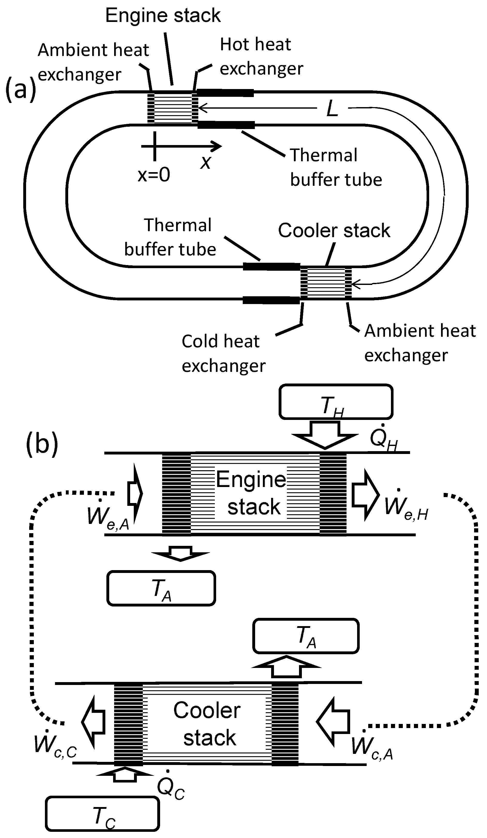
In 2001, Yazaki et al. constructed and tested a thermoacoustic cooling system that has no moving parts and can be driven by various types of heat sources such as sunlight and waste heat [1]. As shown schematically in Figure 1a, their system is composed of a looped tube, an engine stack, a cooler stack, and four heat exchangers. The stacks include several narrow flow channels and are sandwiched by two heat exchangers. Experimental results indicated that an increase in the temperature of the hot heat exchanger (see Figure 1) spontaneously produces an acoustic wave due to the thermoacoustic effect [2,3] and the wave travels in the looped tube. The acoustic wave causes a thermoacoustic heat-pumping effect [2] in the cooler stack (see Figure 1), such that the temperature of the cold heat exchanger decreases. Additionally, Yazaki et al. measured the acoustic pressure and velocity along the looped tube and experimentally demonstrated that both the excitation of the acoustic wave and the thermoacoustic heat pumping are performed through thermodynamic cycles in a manner similar to Stirling and reversed Stirling cycles [4], respectively. These cycles are known to be inherently reversible, and, thus, it is expected that the cooler becomes an efficient system.
The thermoacoustic cooling system constructed by Yazaki et al. includes the engine and cooler stacks in the looped tube as previously mentioned. It is widely known that the design parameters of a stack, such as the flow channel radius and the installation position, affect the efficiency of thermoacoustic energy conversions [5,6,7,8]. Furthermore, there is a possibility that the parameters interact with each other in the thermoacoustic cooling system. Thus, it is necessary to simultaneously optimize the parameters of the engine and cooler stacks to improve the performance of the system. However, there is a paucity of extant studies in which the optimization of the previously mentioned parameters is applied.
In this study, we have numerically investigated the performance of the thermoacoustic cooling system shown in Figure 1 by using the thermoacoustic theory initially proposed by Rott [9,10] and advanced by Swift [2] and Tominaga [3,11]. The efficiency of the engine stack, coefficient of performance (COP) of the cooler stack, and acoustical transmission loss along the looped tube were calculated by changing three parameters, namely the flow channel radius in the engine stack, the flow channel radius in the cooler stack, and the relative position between the stacks. The results indicated that the total efficiency that is defined as the ratio of the cooling power and input thermal power became 0.40 when the three parameters were optimized. This value corresponds to 13% of the thermodynamically ideal value and implies that the efficiency of the engine stack became 75% of Carnot’s efficiency, the COP of the cooler stack became 53% of Carnot’s COP, and the efficiency of the looped tube as an acoustical power transmission line became 33%.
The next section presents the model of the thermoacoustic cooling system. The following section describes the definitions of the evaluated values showing the performance of the engine and cooler stacks and the loss of the looped tube. Then, the numerical method to calculate the values is shown. Finally, the calculation results and discussion are presented.
2. Calculation Model
Figure 1a shows a schematic calculation model, based on a figure in a previous study [1]. The values of design parameters, such as the length of the tubes, were set based on those of Yazaki’s experimental set up [1]. The total length of the looped tube was set as 2.8 m, its inner diameter was set as 40 mm, and the looped tube was filled with a 501 kPa helium gas. One of the stacks was sandwiched by hot and ambient heat exchangers, and it worked as an engine stack. The other stack was sandwiched by ambient and cold heat exchangers, and it worked as a cooler stack. The length of both the stacks corresponded to 40 mm. The distance between the two stacks is denoted as L (see Figure 1a) and was used as one of the parameters with respect to which the performance of the system was varied. Both the stacks were modelled as an array of circular channels. The radius of the circular channels in the engine stack is denoted as , while the radius in the cooler stack is denoted as .
The temperatures of the hot, ambient, and cold heat exchangers are denoted as , , and , respectively. The values of and in the numerical calculation were fixed at 301 K and 251 K, respectively. The temperatures ( and ) are close to the temperatures obtained by Yazaki et al. [1]. However, the value of was determined as one of the calculation results. Each heat exchanger was modelled as a series of parallelly stacked flat plates, with the space between plates corresponding to 1.0 mm and the height corresponding to 10 mm. Two thermal buffer spaces existed along the looped tube. One of the spaces was located at the vicinity of the hot heat exchanger and the temperature changed from to . The other space was located at the vicinity of the cold heat exchanger and the temperature changed from to (see Figure 1).
3. Evaluated Performance
In order to understand thermoacoustic devices, it is necessary to elucidate the power associated with acoustic wave propagation [12]. This is because an acoustic wave causes pressure, density, and temperature changes in thermoacoustic devices, and these are indispensable for energy conversion between heat and work. Furthermore, an acoustic wave transports energy [2,13]. In this section, the definition of the power is presented, and then the efficiency of the engine stack and the coefficient of performance of the cooler stack are expressed by the power.
3.1. Acoustically Transported Power
The time-averaged rate of acoustically-transported mechanical energy is denoted as acoustic power [W], while the time-averaged rate of acoustically-transported thermal energy is denoted as acoustical thermal power [W] [12]. Acoustic power and acoustical thermal power are expressed by oscillatory pressure P and the cross-sectional mean of oscillatory velocity, U, and they are given in Equations (1) and (2) [2,13] as follows:
In the two equations, the tilde refers to complex conjugation, x denotes the axial coordinate along the looped tube, A denotes cross-sectional area of the tube, denotes time-averaged gas temperature, and , , , and denote mean density, specific heat ratio, specific heat at constant pressure, and Prandtl number of the working gas, respectively. Additionally, and represent the thermoacoustic functions that depend on the ratio of the radius r of the flow channel(s) and the penetration depth [3], where is given by , in which denotes angular frequency of the acoustic wave, and denotes thermal conductivity of the working gas. In the study, it is assumed that the heat capacity of the tube wall significantly exceeds that of the working gas. This assumption allows setting the value of the tube-wall temperature constant.
3.2. Efficiency and Coefficient of Performance
In Figure 1b, the thermoacoustic cooler is schematically re-illustrated from a thermodynamical point of view. The subscripts e, cA, H, and C denote engine stack, cooler stack, ambient end, hot end, and cooler end, respectively. For example, denotes acoustic power at the ambient end of the engine stack. Yazaki et al. demonstrated [1] that, when the temperature exceeds a critical value, the gas inside the looped tube including inside the stacks spontaneously oscillates. As a result, the spontaneously generated acoustic wave travels along the looped tube and transports energy. The acoustic power of the generated acoustic wave is input from the ambient end of the engine stack and is amplified in the engine stack. The amplified acoustic power is emitted from the hot end of the engine stack. Therefore, the gain in the acoustic power of the engine stack, , is expressed as Equation (3) as follows:
In order to amplify the acoustic power, it is necessary for the hot heat exchanger to supply acoustical thermal power . Hence, the efficiency of the engine stack is expressed as Equation (4) as follows:
A part of acoustic power is dissipated along the tube between the hot heat exchanger attached to the engine stack and the ambient heat exchanger attached to the cooler stack. The remainder of , denoted as , enters the cooler stack from its ambient side. This is used to pump heat from the cold to ambient heat exchangers along the cooler stack. Subsequently, is output from the cold heat exchanger. The acoustic power is also dissipated in the other part of the looped tube between the cold heat exchanger of the cooler stack and the ambient heat exchanger of the engine stack. The thermal power pumped from the cold heat exchanger is defined as . Because the acoustic power used in the cooler stack is , the coefficient of performance of the cooler stack is expressed as
Acoustic power is delivered to the ambient end of the engine stack and is re-amplified. The efficiency of the looped tube as a transmission line of acoustic power is defined as follows:
When , dissipation does not occur along the tube with the exception of the engine and cooler stacks, and all of the generated acoustic power in the engine stack is utilized in the cooler stack.
The total coefficient of the performance of the total cooler system is expressed as follows:
It is also expressed by using , , and as follows:
4. Numerical Method
This section describes the equations used in the numerical calculation and the method to calculate the performance of the thermoacoustic cooling system.
4.1. Equations
As previously mentioned, and are expressed by P and U, and the efficiency of the energy conversion that occurs in the stacks depends on the acoustic impedance . Hence, , , , and depend on the distributions of P and U. Therefore, P and U are calculated at a given point along the looped tube.
The cooler is divided into the ten components and the two equations are computationally integrated [14] along each component. The value of is important in performing the integration. Two temperature conditions are used, namely that is assumed to be constant and that is calculated based on the assumption that the tube is insulated from its surroundings. In order to satisfy this insulation assumption in the calculation, it is necessary for the value of the enthalpy flow along an insulated tube to be constant [2]. According to Rott [10], is expressed as
4.2. Calculation Procedure
The calculation flow chart is shown in Figure 2 and is described as follows:
- The flow channel radii ( and ) of the engine and cooler stacks and the relative position of the cooler stack, , were set. It should be noted that the temperature of the hot end of the engine stack, , was determined as a result of the calculation, while temperatures ( and ) were fixed as follows: K and K.
- The stability limit condition under which the spontaneous gas oscillation becomes neutral was calculated by using the transfer matrix method [14] (This method is described in Appendix A in detail). As a result of this calculation, , , , and were obtained. It should be noted that, in this step, the values of the temperature gradient along the engine stack, the cooler stack, and the thermal buffer tubes were assumed as linear.
- The obtained combinations of pressure and velocity were used to calculate the acoustic power at the ends of the engine and cooler stacks, (, , , and ). Furthermore, the acoustical thermal power at the hot end of the engine stack and at the cold end of the cooler stack ( and ) were calculated by using the calculated and and Equation (11). It should be noted that the enthalpy flow along the engine stack and that along the cooler stack were already obtained in the third step.
Given that all the equations used are linear, their solution includes integral constants. Subsequently, it is not possible to determine the absolute values of P and U. However, their relative values can be obtained. Therefore, the values of P and U were calculated with the boundary condition of the looped tube (see Appendix A) and the condition kPa. It should be noted that the evaluated performance was determined as a dimensionless value, and, thus, the pressure amplitude did not impact the results.
5. Result and Discussion
In this section, first the validation of the present numerical method is presented. Then, the optimization of the distance between the two stacks is described and the physical reason of the effect of the distance on the performance is discussed. Finally, the simultaneous optimization of the radii of the engine and cooler stacks is shown.
5.1. Acoustic Field
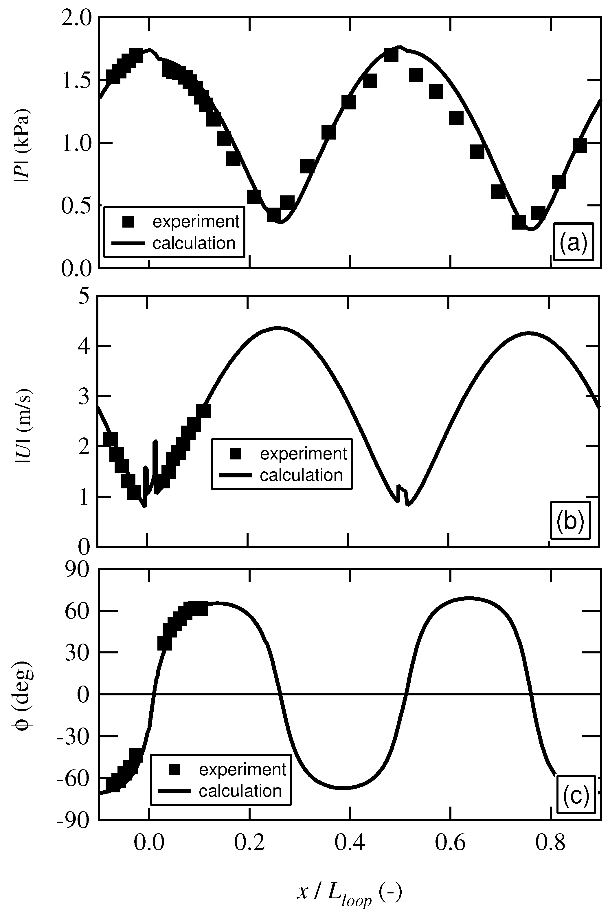
Yazaki et al. provided the experimentally measured acoustic field in the looped tube but did not demonstrate the performance such as COP [1]. Hence, in order to show the validation of the present numerical method, we calculated pressure and velocity along the looped tube and compared them with the experimental results obtained by Yazaki.
In Figure 3, the numerically obtained , , and argument of the acoustic impedance , , along the looped tube are denoted by solid lines with the experimental results (symbols). It should be noted that, following the experimental conditions outlined by Yazaki, the second stack worked as a load without ambient and cold heat exchangers, the working gas corresponded to atmospheric air, and the pressure amplitude at the ambient end of the engine stack was set as 1.7 kPa in this calculation. In addition to these, we should note that Yazaki et al. plotted the argument of in their article [1]. As shown in the figure, a good agreement was obtained between the numerical and experimental results. Several extant studies [17,18] indicated that, when P and U are correctly calculated, the calculated and are then in good agreement with the experiment. Hence, it is considered that the present numerical method can be used to simulate the performance of the cooler.
5.2. Effect of the Relative Position of the Cooler Stack
Yazaki et al. reported that the position of the cooler stack influences the performance of the system [1]. Therefore, the relative position was changed. The radius of the narrow channels of the engine and cooler stacks was set as 0.27 mm, which corresponds to the same value as that in Yazaki’s experimental setup [1]. Given this value, in the stacks approximately corresponds to 1.5 at K.
The calculated results with one-wavelength mode ( Hz) are shown in Figure 4. The results indicated that the efficiency of the engine and the coefficient of performance of the cooler COP depended on the relative position and that the maximum value of and that of COP corresponded to 0.31 and 2.45 at , respectively. These values are 1.9 and 105 times larger than the values of and COP at , respectively. Given that corresponds to 2.8 m, the difference between 0.54 and 0.50 times of corresponds to 0.11 m. Hence, it is considered that the optimization of is significant in increasing the performance of the cooler. Conversely, as shown in Figure 4c monotonically decreased from 0.46 to 0.21, when was increased from 0.50 to 0.56. This means that there is a tradeoff between the dependence of on and those of and COP when . As the dependence of was weak when compared to that of the COP, the COP became maximum ( 0.21) at , as shown in Figure 4d. This result is consistent with that in the study by Yazaki et al. [1].
Additionally, P and U were calculated along the looped tube and the results revealed that the distributions of P and U were not fixed but were influenced by . Figure 4e,f show and at the ends of the engine and cooler stacks as a function of , where a is the adiabatic sound speed and is the argument of . As indicated by the open triangles in Figure 4e, in the engine stack corresponded to a maximum at . This contributes to the maximum obtained at because high decreases the viscous loss. It is also found that s at both of the ends of the engine stack took negative values above , as indicated by open-circles and squares in Figure 4e. This means that was negative along the engine stack. This result also contributes to the increase of [19]. This is because the energy conversion caused by the standing wave works positively only when , whereas the energy conversion caused by the traveling wave works positively when (as shown in Equations (12) and (13) in the previous study [3]). In the cooler stack, weakly depended on , whereas depended on as shown in Figure 4f. At , at which COP became maximum, was not near zero but close to 60. We consider the discrepancy between the optimum for the cooler stack and that for the engine stack can be attributed to the difference of the temperature gradient along them: the temperature gradient along the cooler stack was much lower than that along the engine stack. The standing wave component works well in the cooler stack when compared with that in the engine stack because the thermal power that is transported by the “Dream Pipe Effect” [3] and corresponds to major loss sources in standing wave thermoacoustic coolers and engines, is proportional to the temperature gradient (as shown in Equation (17) in the previous study [3]). Therefore, it is considered that, given that the temperature gradient was small and depended weekly on , COP was maximum at , where was not close to 0 but close to 60. It should be noted that when is positive, the thermal power pumped by the standing wave component is directed from the cold end to the ambient end of the cooler stack (as shown in Equation (16) in the previous study [3]).
To consider the dependence of on , the ratio of and is shown as a function of in Figure 4g. Here, and are the maximum and minimum values of the pressure amplitude in the looped tube. As predicted by de Block [20], the traveling wave like field, in which is near unity, transports acoustic power more efficiently than the standing wave like field, in which is much larger than unity. As can be seen from Figure 4c,g, when was small, was large as expected. Therefore, it can be said that when was increased from 0.50 to 0.56, the acoustic field formed in the looped tube was changed from a traveling wave like field to a standing wave like one, and then the efficiency of the tube, , was decreased.
Figure 4h shows the calculated temperature of the hot heat exchanger on the engine stack, . The results indicate that reduced when decreased from 0.56 to 0.50. Nevertheless, this is not a good design choice as COP became close to zero at as mentioned above.
5.3. Optimization of Radii in Stacks
At where COP corresponded to a maximum, corresponded to 674 K as shown in Figure 4e. Given that and were set to 301 K and 251 K, respectively, the thermodynamic upper limit of , namely Carnot’s efficiency is as follows:
Additionally, Carnot’s COP is as follows:
Hence, and COP corresponds to 0.55 and 5.0, respectively. This implies that the calculated maximum and COP corresponds to 57% and 49% of the Carnot’s values, respectively. It was considered that there was some scope for improvement with respect to these values.
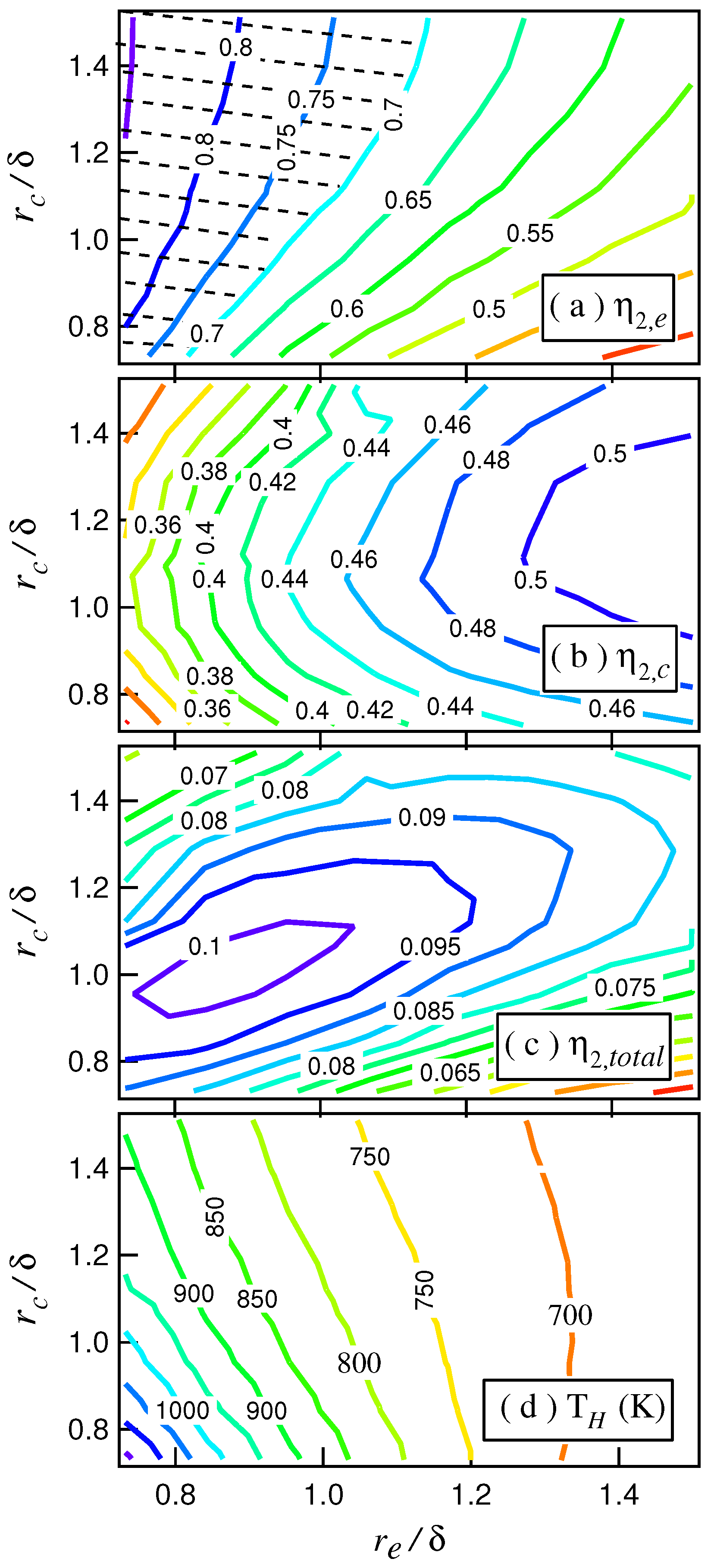
It is widely known that the radius of a stack influences the efficiency of the energy conversion caused by an acoustic wave [8]. Hence, the calculation described in Section 4.2 was performed by varying and and keeping and K. In order to compare the obtained , COP, and COP with their thermodynamic upper limit values, the efficiencies are defined in the following equations:
As shown in the contour plot of Figure 5a, improved when and were decreased and increased, respectively. The plot also shows that exceeded 70% when and were determined as the values in the hatched area of Figure 5a. The value of was comparable to the efficiency of the most efficient thermoacoustic and Stirling engines constructed to date [15,21,22]. Conversely, increased with increasing in the calculated ranges as shown in Figure 5b. This is opposite to the dependence of on . Hence, it is difficult to simultaneously achieve high and by controlling for and . Furthermore, and should be optimized simultaneously. In order to consider the reason as to why the decrease of caused an improvement in and the deterioration in , the acoustic impedance Z was re-calculated at the engine and cooler stacks. The results indicated that a decrease in increased at the engine stack and decreased at the cooler stack. This is caused by the fact that when was decreased, the sweet spot area was narrowed, in which is high and the argument of Z is near zero [23], and, then, the position of the cooler stack departed from the sweet spot area. This implied that the optimum relative position shifted toward . Hence, after considering the optimum values of and , the relation between and was re-calculated.
In Figure 5c, the contour plot of the calculated is shown as a function of and . It is possible to determine the optimum point to increase . With respect to the optimum point (, ), was approximately 10%. As shown in Figure 5d, the temperature increased when and decreased. This means that, in the case where the value of is determined as a given condition, such as in the case of the utilization of waste heat, the optimum and depend on the given value.
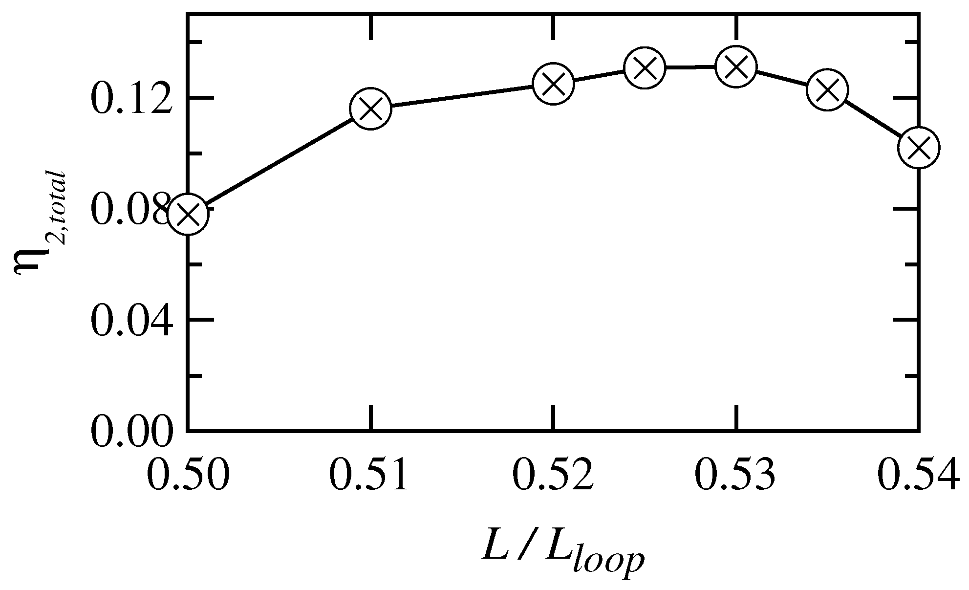
As described above, the results indicated that the optimum relative position changed when decreased. The values of and were set to the optimum values, namely 0.95 and 1.06, respectively, and was calculated as a function of . As shown in Figure 6, the optimum corresponded to 0.53, and this indicates a slight shift from 0.54. At this point, , , , and corresponded to 13%, 75%, 53% and 33%, respectively. This means that increased when was retained as a relatively high value as expected. However, the value of was still low when compared with the others. It is considered that it is important to determine ways to improve for practically using the looped tube thermoacoustic system with two stacks.
6. Conclusions
In this study, the performance of a thermoacoustic system with an engine and cooler stacks was numerically investigated by changing the radii of the two stacks and the relative position between the stacks. The results indicated that the three parameters interact with each other, and they must be simultaneously optimized to increase the performance. Three steps were performed for the optimization. First, the relative position was optimized by keeping the values of the radii at a constant value. Second, the radii were optimized by maintaining the optimum relative position at a constant value. Finally, the relative position was re-optimized. The result of the optimization of the parameters revealed that the total COP corresponds to 0.40, which is 13% of the thermodynamical upper limit value.
Acknowledgments
The authors would like to acknowledge the Indonesian government for its financial support. In addition, the authors would like to thank the reviewers for very useful comments and suggestions.
Author Contributions
Irna Farikhah performed the numerical calculations; Irna Farikhah and Yuki Ueda analyzed the results; Yuki Ueda wrote the draft of the manuscript; Irna Farikhah and Yuki Ueda revised the manuscript; Both authors read and approved the final manuscript.
Conflicts of Interest
The authors declare no conflict of interest.
Appendix A. Transfer Matrix Method
In this Appendix, the method to calculate the stability limit is described [14]. Equations (9) and (10) are modified in a matrix form as follows:
A forward different scheme using the fourth-order Runge–Kutta method to Equation (A1) is applied to obtain the following expressions:
where E denotes a unit matrix. When the value of is known and a flow channel is uniform, we can numerically integrate Equation (A2) and obtain the following expression:
Here, n denotes the number of partitions between and x, is defined as , and represents at .
The thermoacoustic cooler shown in Figure 1 was divided into the ten components. Their names and numbers are defined as follows: (1) the engine stack, (2) the hot heat exchanger, (3) the thermal buffer tube A, (4) the waveguide A, (5) the ambient heat exchanger A, (6) the cooler stack, (7) the cold heat exchanger, (8) the thermal buffer tube B, (9) the waveguide B, and (10) the ambient heat exchanger B. The numerical integration along each component was performed and their transfer matrices were obtained. The total flow-path areas in the components are different from each other, and thus the connecting matrix is as follows:
where A denotes the total-path area and the subscripts k and l denote the number of the components. The transfer matrices of the components and the connecting matrices are used to express the transfer matrix of the total system as follows:
Additionally, was used such that the pressure and velocity at the ambient end of the engine stack corresponds to the same as follows:
The solution (, ) of Equation (A6) is nonzero if the determinant of the matrix () is zero, i.e., if the following expression is applicable:
where E denotes the unit matrix and denotes the element of . Therefore, Equation (A7) was numerically solved to achieve the condition of the stability limit of the spontaneous gas oscillation induced in the thermoacoustic cooler.
References
- Yazaki, T.; Biwa, T.; Tominaga, A. A piston-less Stirling cooler. Appl. Phys. Lett. 2002, 80, 157–159. [Google Scholar] [CrossRef]
- Swift, G.W. Thermoacoustics A Unifying Perspective for Some Engines and Refrigerators; Acoustical Society of America: New York, NY, USA, 2002. [Google Scholar]
- Tominaga, A. Thermodynamic aspects of thermoacoustic theory. Cryogenic 1995, 35, 427–440. [Google Scholar] [CrossRef]
- Ceperley, P.H. A piston-less Stirling engine. J. Acoust. Soc. Am. 1979, 66, 1508–1513. [Google Scholar] [CrossRef]
- Timoumi, Y.; Tlili, I. Performance optimization of Stirling engines. Renew. Energy 2008, 33, 2134–2144. [Google Scholar] [CrossRef]
- Tlili, I. Finite time thermodynamic evaluation of endoreversible Stirling heat engine at maximum power conditions. Renew. Sustain. Energy Rev. 2012, 16, 2234–2241. [Google Scholar] [CrossRef]
- Tijani, M.E.H.; Zeegers, A.D.W.J.C.H. Design of thermoacoustic refrigerators. Cryogenic 2002, 42, 49–57. [Google Scholar] [CrossRef]
- Ueda, Y.; Bassem, M.M.; Tsuji, K.; Akisawa, A. Optimization of the regenerator of a travelling-wave thermoacoustic refrigerator. J. Appl. Phys. 2010, 107, 034901. [Google Scholar] [CrossRef]
- Rott, N. Damped and thermally driven acoustic oscillations in wide and narrow tubes. Z. Angew. Math. Phys. 1969, 20, 230–243. [Google Scholar] [CrossRef]
- Rott, N. Thermally driven acoustic oscillations part II: Stability limit for helium. Z. Angew. Math. Phys. 1973, 24, 54–72. [Google Scholar] [CrossRef]
- Tominaga, A. Fundamental Thermoacoustic; Uchidarokakumo: Tokyo, Japan, 1998. [Google Scholar]
- Swift, G.W. Springer Handbook of Acoustics: Thermoacoustics; Springer: New York, NY, USA, 2006; Chapter 7. [Google Scholar]
- Rott, N. Thermally driven acoustic oscillations, part III: Second-order heat flux. Z. Angew. Math. Phys. 1975, 26, 43–49. [Google Scholar] [CrossRef]
- Ueda, Y.; Kato, C. Stability analysis of thermally induced spontaneous gas oscillations in straight and looped tubes. J. Acoust. Am. 2008, 124, 851–858. [Google Scholar] [CrossRef] [PubMed]
- Swift, G.W.; Gardner, D.L.; Backhaus, S. A thermoacoustic Stirling engine. Nature 1999, 399, 335–338. [Google Scholar]
- Biwa, T.; Tashiro, Y.; Ishigaki, M.; Ueda, Y.; Yazaki, T. Measurements of acoustic streaming in a looped-tube thermoacoustic engine with a jet pump. J. Appl. Phys. 2007, 101, 064914. [Google Scholar] [CrossRef]
- Backhaus, S. A thermoacoustic-Stirling heat engine: Detailed study. J. Acoust. Soc. Am. 2000, 107, 3148–3166. [Google Scholar] [CrossRef] [PubMed]
- Bassem, M.M.; Ueda, Y.; Akisawa, A. Design and construction of a travelling wave thermoacoustic refrigerator. Int. J. Refrig. 2011, 34, 1125–1131. [Google Scholar] [CrossRef]
- Yazaki, T.; Iwata, A.; Maekawa, T.; Tominaga, A. Traveling wave thermoacoustic engine in a looped tube. Phys. Rev. Lett. 1998, 81, 3128. [Google Scholar] [CrossRef]
- De BloK, K. Muti-stage traveling wave thermoacoustics in practice. In Proceedings of the 19th International Congress on Sound and Vibration (ICSV 19), Vilnius, Lithuania, 8–12 July 2012; pp. 1–8. [Google Scholar]
- Tijani, M.E.H.; Spoelstra, S. A high performance thermoacoustic engine. J. Appl. Phys. 2011, 110, 093519. [Google Scholar] [CrossRef]
- Timoumi, Y.; Tlili, I.; Nasrallah, S.B. Design and performance optimization of GPU-3 Stirling engines. Energy 2008, 33, 1100–1114. [Google Scholar] [CrossRef]
- Gardner, D.L.; Swift, G.W. A cascade thermoacoustic engine. J. Acoust. Soc. Am. 2003, 114, 1905. [Google Scholar] [CrossRef] [PubMed]
Figure 1.
A thermoacoustic system with engine and cooler stacks [1] in a looped tube.
Figure 1.
A thermoacoustic system with engine and cooler stacks [1] in a looped tube.

Figure 2.
Flow chart for evaluating , COP, , and COP.
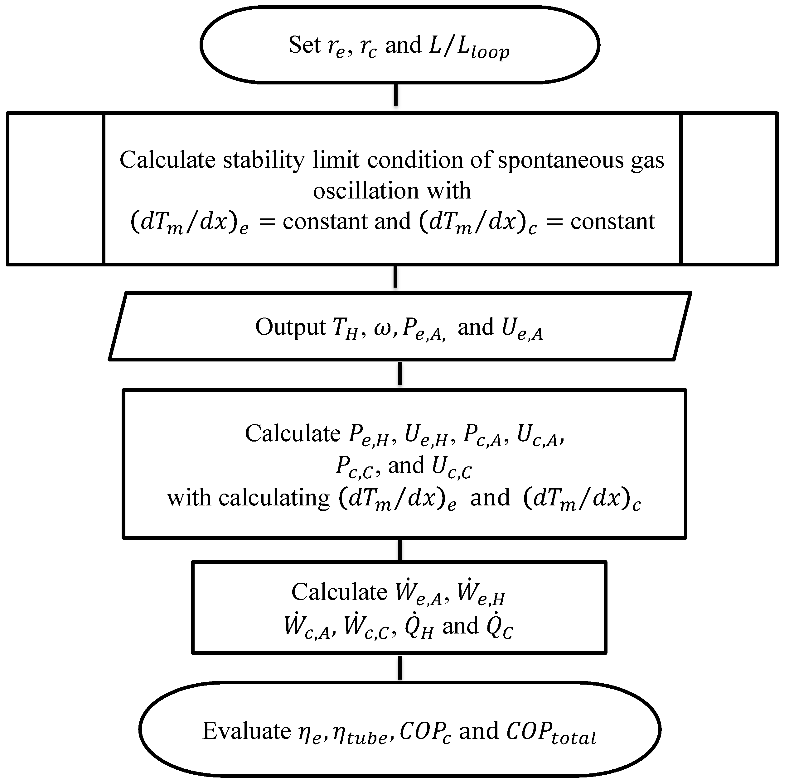
Figure 3.
, , and as a function of . The symbols show the experimental results obtained from the article [1].
Figure 3.
, , and as a function of . The symbols show the experimental results obtained from the article [1].

Figure 4.
, COP, , COP, , , and as a function of .
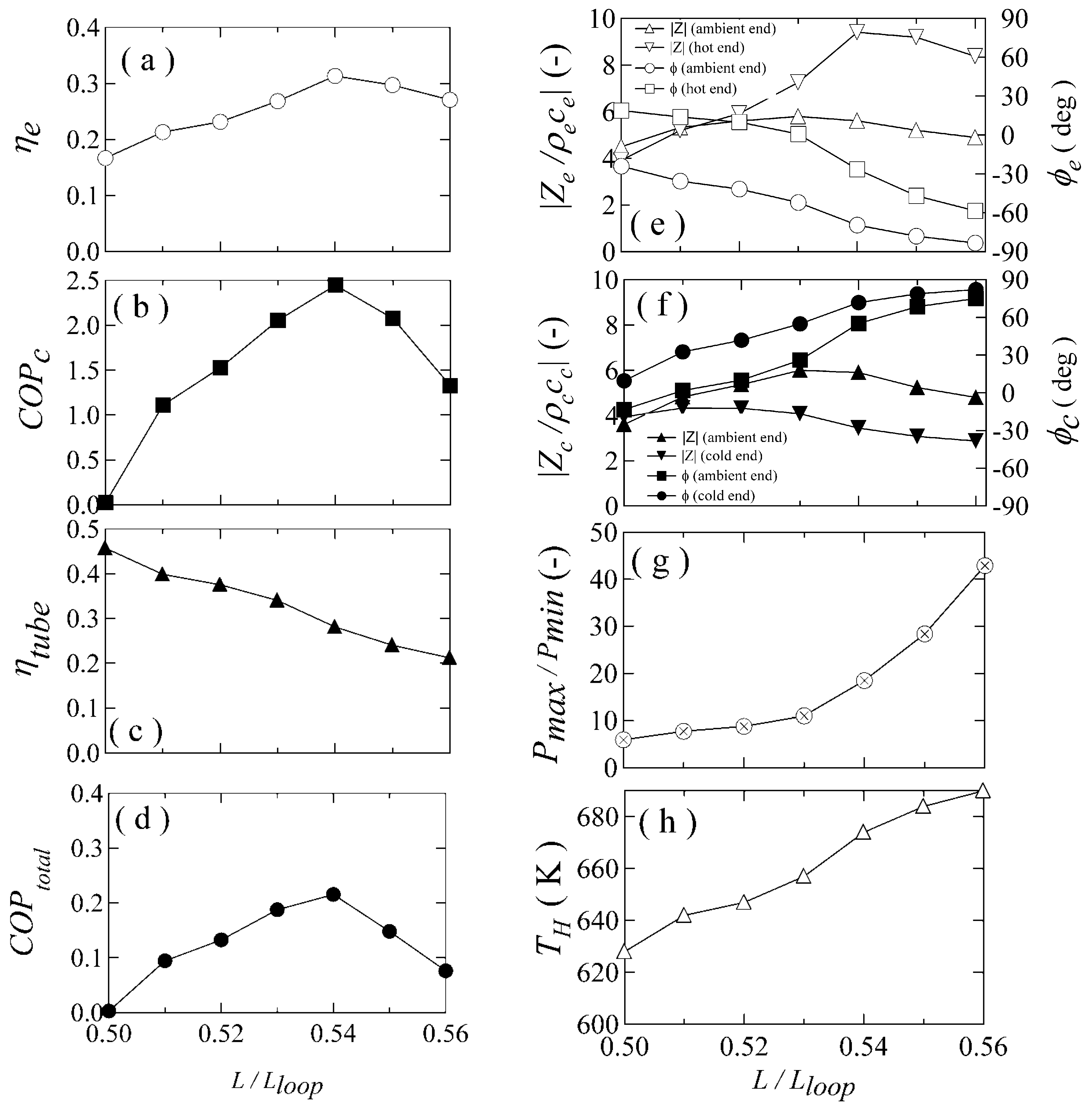
Figure 5.
, , , and as a function of and .

Figure 6.
The total efficiency as a function of . The value of is calculated with the optimum and , which are determined based on the results shown in Figure 5c.
Figure 6.
The total efficiency as a function of . The value of is calculated with the optimum and , which are determined based on the results shown in Figure 5c.
© 2017 by the authors. Licensee MDPI, Basel, Switzerland. This article is an open access article distributed under the terms and conditions of the Creative Commons Attribution (CC BY) license (http://creativecommons.org/licenses/by/4.0/).
Share and Cite
MDPI and ACS Style
Farikhah, I.; Ueda, Y. Numerical Calculation of the Performance of a Thermoacoustic System with Engine and Cooler Stacks in a Looped Tube. Appl. Sci. 2017, 7, 672. https://doi.org/10.3390/app7070672
AMA Style
Farikhah I, Ueda Y. Numerical Calculation of the Performance of a Thermoacoustic System with Engine and Cooler Stacks in a Looped Tube. Applied Sciences. 2017; 7(7):672. https://doi.org/10.3390/app7070672
Chicago/Turabian StyleFarikhah, Irna, and Yuki Ueda. 2017. "Numerical Calculation of the Performance of a Thermoacoustic System with Engine and Cooler Stacks in a Looped Tube" Applied Sciences 7, no. 7: 672. https://doi.org/10.3390/app7070672
Note that from the first issue of 2016, this journal uses article numbers instead of page numbers. See further details here.