
Numerical Predictions of Early Stage Turbulence in Oscillatory Flow across Parallel-Plate Heat Exchangers of a Thermoacoustic System

1
Centre for Advanced Research on Energy, Faculty of Mechanical Engineering, Universiti Teknikal Malaysia Melaka, Hang Tuah Jaya, Durian Tunggal, Melaka 76100, Malaysia
2
Faculty of Engineering, University of Leeds, Woodhouse Lane, Leeds LS2 9JT, UK
*
Author to whom correspondence should be addressed.
Appl. Sci. 2017, 7(7), 673; https://doi.org/10.3390/app7070673
Submission received: 19 April 2017
/
Revised: 22 May 2017
/
Accepted: 31 May 2017
/
Published: 30 June 2017
(This article belongs to the Special Issue Heat Transfer Processes in Oscillatory Flow Conditions)
Abstract
:This work focuses on the predictions of turbulent transition in oscillatory flow subjected to temperature gradients, which often occurs within heat exchangers of thermoacoustic devices. A two-dimensional computational fluid dynamics (CFD) model was developed in ANSYS FLUENT and validated using the earlier experimental data. Four drive ratios (defined as maximum pressure amplitude to mean pressure) were investigated: 0.30%, 0.45%, 0.65% and 0.83%. It has been found that the introduction of the turbulence model at a drive ratio as low as 0.45% improves the predictions of flow structure compared to experiments, which indicates that turbulent transition may occur at much smaller flow amplitudes than previously thought. In the current investigation, the critical Reynolds number based on the thickness of Stokes’ layer falls in the range between 70 and 100. The models tested included four variants of the RANS (Reynolds-Averaged Navier–Stokes) equations: k-ε, k-ω, shear-stress-transport (SST)-k-ω and transition-SST, the laminar model being used as a reference. Discussions are based on velocity profiles, vorticity plots, viscous dissipation and the resulting heat transfer and their comparison with experimental results. The SST-k-ω turbulence model and, in some cases, transition-SST provide the best fit of the velocity profile between numerical and experimental data (the value of the introduced metric measuring the deviation of the CFD velocity profiles from experiment is up to 43% lower than for the laminar model) and also give the best match in terms of calculated heat flux. The viscous dissipation also increases with an increase of the drive ratio. The results suggest that turbulence should be considered when designing thermoacoustic devices even in low-amplitude regimes in order to improve the performance predictions of thermoacoustic systems.
1. Introduction
Oscillatory wall-bounded flow emerges in a variety of engineering applications, one of the good examples being thermoacoustic devices. These are known as a technology that offers greener alternatives for energy conversion applications in areas such as waste heat recovery, solar power or environmentally-friendly cooling technologies. One of the keys to a better design of thermoacoustic systems lies in the understanding of the flow and heat transfer within the internal structures in oscillatory conditions. Experimental studies often reveal signs of nonlinearities that are insufficiently addressed by the linear models typically used for design predictions [1,2]. These may be a result of phenomena such as acoustic streaming, vortex shedding or turbulence in the flow [3,4,5].
Previous studies of oscillatory flows identified many interesting features of the transition process [6,7,8,9]. The resulting turbulent flow is characterised by the sudden, explosive appearance of turbulence towards the end of the acceleration phase of the cycle. Turbulent flow is sustained throughout the deceleration phase, while during the early stages of the acceleration phase, the production of turbulence essentially stops, and velocity profiles agree with laminar theory [8]. Nevertheless, during this period, the disturbances retain a small, but finite energy level.
Theoretical [1,10] and numerical [11,12,13,14,15] works related to thermoacoustic processes typically assume a laminar flow (limited to low drive ratios). The critical Reynolds numbers for the transition to turbulence in an oscillatory flow are reviewed by Ohmi et al. [6]. Their experimental results agree with the critical value of 400 of the Reynolds number defined by Merkli and Thomann [7] based on the Stokes layer thickness. The flow regions are categorised into laminar, transitional and turbulent. However, oscillatory flows of a Reynolds number higher than 400 are shown experimentally to experience a stage of relaminarization where the velocity profiles match the laminar prediction during the initial stage of the acceleration phase and change to turbulent-like profiles at the later phase, before turning back to laminar [8,9].
An additional complication in the transition/relaminarization processes lies in the appearance of temperature-dependent fluid properties, compressibility effects or additional forces, such as gravity [8]. Therefore, necessary precautions need to be taken in the modelling of such flow. As for the size of the computational domain, Fieldman and Wagner [13] suggested that the length of the domain should not be too short or too long. The former alters turbulence characteristics while the latter can result in relaminarization. These observations were made for a turbulent oscillatory flow inside a pipe. They may not be directly applicable to oscillatory flow across parallel-plate structures, but these ideas need to be borne in mind.
Experimental work reported by Shi et al. [16,17] has shown that the introduction of a temperature distribution along the fins (compared to isothermal situation) results in flow asymmetry within the channels and in the immediate vicinity outside and temperature-driven buoyant flow, giving rise to convective currents some distance away from the plates. The flow asymmetry observed through the velocity profiles shown in [17] may be related to the temperature-dependent properties of the fluid and additional flow forcing due to natural convection.
Piccolo [12] performed numerical studies of the heat exchanger arrangement of Shi et al. [17] and further comparisons between experiment and CFD were made in [18]. The laminar model was limited only to the area between the heat exchanger plates and neglected the gravity effects. The natural convection observed in the experiment was modelled as “heat loss” by introducing a fictitious heat sink and heat source next to the heat exchangers. This approach provides a general idea about the magnitude of heat losses occurring in the experiment. However, detailed investigation needs to be conducted to identify the mechanism that contributes to these losses. Besides, buoyancy forces may also contribute to the nonlinearity of flow in addition to turbulence and streaming [8].
The current understanding of thermoacoustic processes is based on the assumption that the linear acoustic theory developed by Rott [19] is reliable for the flow with the drive ratio (the ratio of oscillating pressure amplitude to mean pressure) of up to 2–3% [1]. However, turbulence may occur at lower drive ratios particularly within the internal structures of thermoacoustic devices, and hence, numerical modelling needs to be improved. There are quite a number of turbulence models available for solving fluid dynamical problems [20]. Unfortunately, there are no strict guidelines as to which model is best for a given case. Modelling turbulence, among others, requires knowledge about the flow physics and the established practice for a specific problem. The correct choice of turbulence model is important to ensure that the physics of flow within practical thermoacoustic systems is properly presented. The objective of this study is to test the performance of widely-available RANS (Reynolds-Averaged Navier–Stokes) turbulence models for the prediction of flow behaviour in oscillatory flow conditions in the presence of the wall temperature gradient, which is a typical situation in heat exchangers of thermoacoustic devices. In addition, studies of viscous dissipation, related to pressure losses in real systems, are carried out, together with surface heat flux calculations to provide additional validation against available experimental results.
2. Computational Model
The computational domain used in this paper is based on the experimental setup of Shi et al. [16,17], sketched at the top of Figure 1. It is a loudspeaker-driven, standing-wave, 8.3 m-long resonator (of which 7.4 m is a constant cross-section square duct of 134 mm × 134 mm). It is filled with nitrogen at atmospheric pressure and operates in the quarter-wavelength mode, with the frequency of 13.1 Hz. The pressure antinode is at the end-wall. The resonator contains a parallel-plate hot heat exchanger (HHX) coupled with a cold heat exchanger (CHX). Overall, there are 10 pairs of individual plates: five pairs are heated/cooled, and five pairs (at the top/bottom) provide a uniform porosity (flow resistance) across the cross-section. The dimensions of the plates and flow channels are shown at the bottom of Figure 1. Point ‘m’ denotes the “joint” where the hot and cold plates meet. It is at from the pressure antinode. The electrical heating elements in HHX and cooling water flow in CHX aim to provide flat temperature profiles over the fins: 200 °C and 30 °C, respectively; but in practice, the heat leaks produce a slightly distorted temperature distribution as reported in [17,21]. Particle image velocimetry (PIV) and planar laser-induced fluorescence (PLIF) techniques provide the oscillatory velocity and temperature field information around the heat exchangers.
Preliminary numerical studies [22] have shown that the pressure and velocity in the flow far away from the heat exchangers can be estimated from the linear thermoacoustic theory. Thus, a “short model” (excluding the rest of the resonator) is acceptable if the incoming/outgoing oscillatory flow does not interfere with the plate structure [11]. The computational domain consists of two regions: the area within the plate structure and two areas outside (i.e., the open areas on the left and right from the plate structure) bounded by the resonator walls. Based on Fieldman and Wagner’s correlation [13], the ratio of length to diameter (L/D) for the case investigated here should not be larger than 11.4 for flow in the channel and less than 0.52 for the flow outside. The computational domain developed based on the length of 270 mm either way from the joint between HHX and CHX (cf. the middle of Figure 1) complies with these requirements. Due to flow asymmetry caused by the natural convection observed in the experiment, the full height covering all 10 pairs of plates is covered by the model.
A quadrilateral structured mesh (cf. the middle of Figure 1) was used. It was refined in both the - and -directions to check for grid independency. The model was tested for cell counts of 47,360, 58,510, 71,460 and 85,560. It was found that the cell count of 71,460 provides a solution that is independent of the grid size and hence used throughout the current study. The minimum orthogonal quality is 0.86 with the maximum skewness of 0.13, which show that the mesh quality is very close to a good quality mesh (close to one for minimum orthogonality and close to zero for maximum skewness) [23]. The nearest node from the wall, +, for all cases is between 0.1 and 1.24. This value differs depending on the drive ratio and flow amplitude during each phase of the flow cycle; and serves as a reference for the resolution of the mesh near the wall.
The models were solved using a high performance computer (4 login nodes, with 28 cores of 56 threads and 256 GB memory per one login node). The calculation for one cycle takes about 30 min. The transient models were calculated until a steady oscillatory condition is achieved, i.e., where pressure, velocity and temperature do not change with time. It was found that all models needed to be calculated for at least 70 cycles to meet this condition (approximately 35 h of computational time). The flow solutions presented in this paper rely on the RANS equations used for turbulence modelling, while the laminar model (see e.g., [21]) is solved for comparisons. The four RANS models tested included: k-ε, k-ω and shear-stress-transport (SST)-k-ω and transition-SST provided by ANSYS FLUENT 13.0 [23]. The RANS equations (shown in index notation) are:
where
These have a form similar to the laminar model of Navier–Stokes equations, but the solution variables now represent the ensemble-averaged (or time-averaged) values. The new terms at the end of Equation (2) are the Reynolds stresses representing the turbulence effect. For compressible flow, the fluctuation of density may affect the turbulence. In this case, the transport equations can be interpreted as Favre-averaged Navier–Stokes equations, with velocities representing the mass-averaged values [20,22]. The effective stress tensor represents the stress tensor under the influence of turbulence with effective viscosity, , defined as a sum of laminar viscosity, , and turbulent viscosity, . Similarly, the effective thermal conductivity, , is the sum of mean thermal conductivity, , and turbulent conductivity, . The turbulent thermal conductivity is calculated as, and the turbulent Prandtl number, , has a constant value of 0.85. The eddy viscosity, , is calculated using the turbulence model.
The Reynolds stresses are solved through additional equations provided by the turbulence model. In this study, turbulence is assumed isotropic so that the Boussinesq hypothesis is applicable to relate the Reynolds stresses to the mean velocity gradient as follows [23]:
The subscripts , and refer to the coordinates , and , respectively. The term, , is known as the turbulent kinetic energy. The Kronecker delta ( if and if ) is introduced to correctly model the normal component of the Reynolds stress [20]. The RANS models used require additional equations to solve for turbulent viscosity, , and turbulent kinetic energy, , to obtain the Reynolds stresses using Equation (5). The Reynolds stresses are then used to correctly model the momentum equation for the turbulence-affected flow through Equation (2).
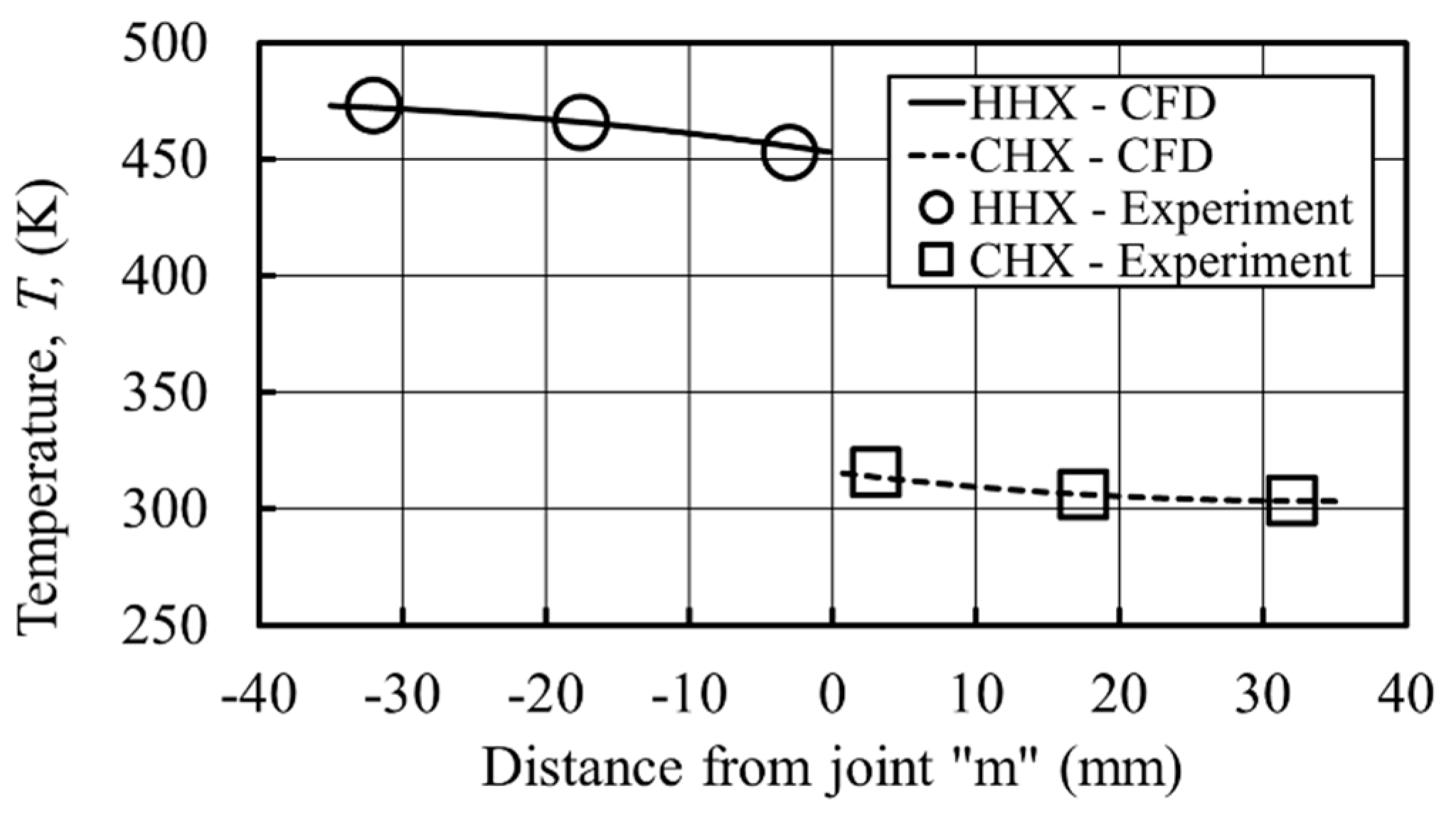
Oscillating pressure, , and mass flux, , are assigned at locations and , respectively (cf. Figure 1), far enough from the heat exchangers. Condition (8) is to ensure that when the flow reverses, its temperature is equal to that of the cells next to the boundary. The wave number, , is constant because the frequency, , is constant. The terms and refer to the speed of sound and the pressure amplitude at the antinode, respectively. The phase, , is set to follow the standing-wave criterion where pressure and velocity are 90° out of phase. The adiabatic non-slip wall was assigned at the resonator walls. The heat exchanger plates were assigned temperature profiles based on experiments [17]. Figure 2 shows the interpolated profiles used in the current work. Nitrogen inside the resonator is modelled as an ideal gas. The viscosity, , and thermal conductivity, of the gas change with temperature, and the equations are given after Abramenko et al. [24] as:
The influence of gravity is modelled with gravitational acceleration set to 9.81 m/s2.
Additional equations, which depend on the type of turbulence model solved, are used to solve Reynolds stresses appearing on the right-hand side of the RANS Equation (2). For all turbulence models tested, additional boundary conditions for the turbulence model are set at the boundaries and by assigning the value of turbulence intensity, , and turbulence length scale, , defined as:
The Reynolds number, , is calculated using the velocity amplitude at location , , obtained from Shi et al. [16,17] and the gap between plates, , as shown in Figure 1. The density, , and viscosity, , used in calculating Equation (10) are taken at 300 K. ANSYS FLUENT 13.0 [23] uses the inputs defined in Equations (10) and (11) to estimate the inlet distributions of turbulence kinetic energy, , and turbulence dissipation, , using the following equations [20,22]:
where is the characteristic flow velocity and is an empirical constant that varies depending on the turbulence model used (approximately 0.09). The sensitivity of the results to these inlet conditions is tested by changing the value of turbulence intensity, , to be the value calculated using the velocity amplitude at the boundaries obtained from the equations of lossless theory. It is found that the solution is insensitive to the turbulence boundary conditions. This shows that the domain is sufficiently long to avoid the interaction between the flow around the plates and the inlet/outlet flows into/out of the domain. Default values are retained for all constants of all models used [23].
A pressure-based solver is used for all models with the application of the pressure-implicit with splitting operators (PISO) algorithm for the pressure-velocity coupling. The second order implicit discretisation scheme is selected for discretisation of time. The transport equations and turbulent equations are solved using the second order upwind scheme. This transient model is calculated with time step size set as per cycle, chosen so that calculations converge within 15–18 iterations in every time step. The model is set to converge at absolute values of 10−4 for all transport and turbulence equations and 10−8 for the energy equation.
3. Results and Discussion
This section presents the numerical results obtained and the relevant discussions. Section 3.1 deals with the preliminary work using the laminar model, while Section 3.2 focuses on solutions of RANS turbulence models studied in this work. Both aspects contain comparisons with earlier experimental results of Shi et al. [16,17]. The subsequent Section 3.3 discusses the numerical investigation of viscous dissipation based on the models that best represent flow behaviour in the drive ratios investigated. Finally, Section 3.4 deals with numerical heat transfer predictions and their comparisons with experimental data.
3.1. Laminar Flow Model
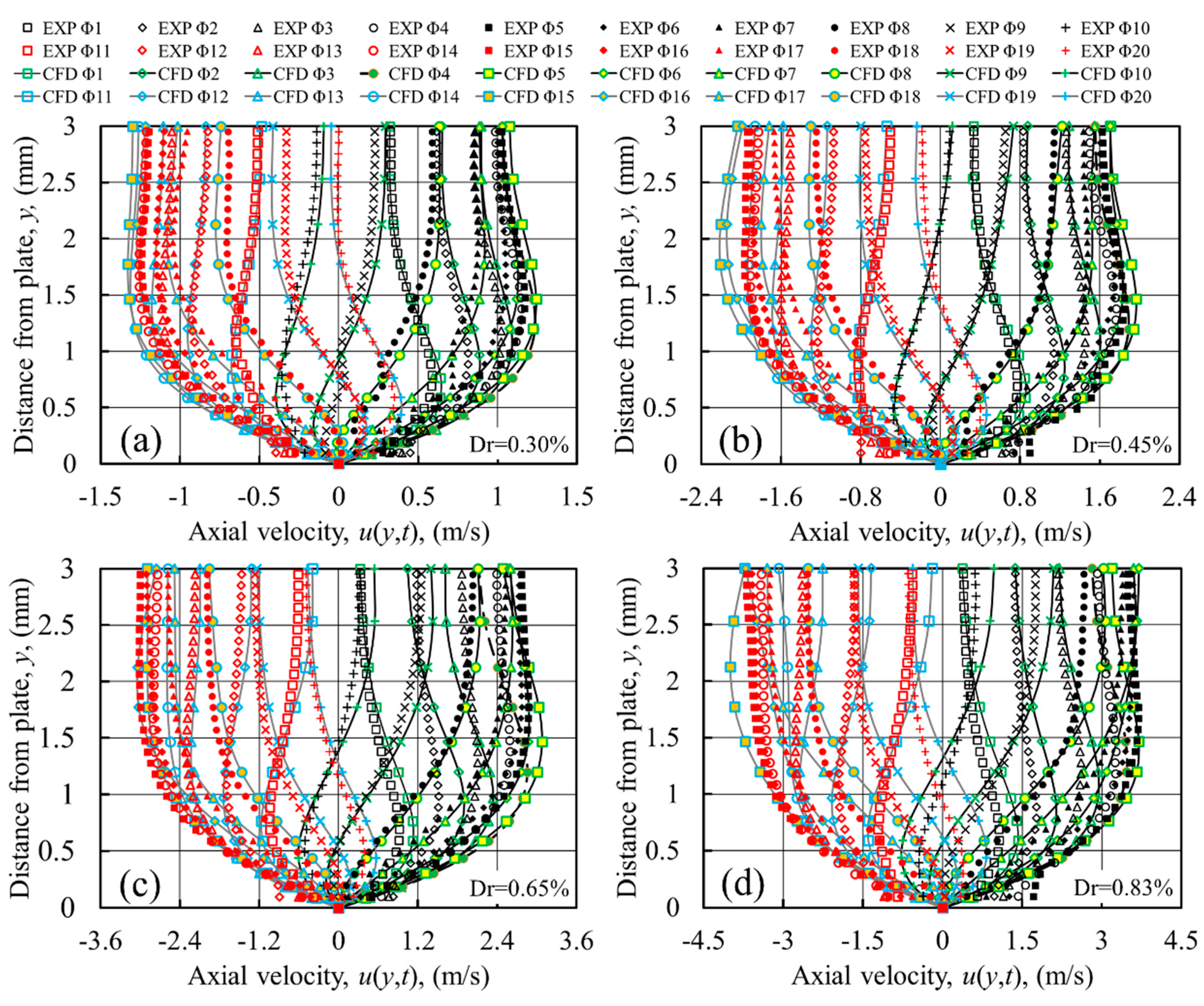
According to Merkli and Thomann [7], an oscillatory flow is considered laminar as long as the Reynolds number (based on the thickness of Stokes’ layer) is less than 400. This is defined as , with , and representing the axial velocity amplitude, viscosity and angular velocity, respectively. The values of the Stokes Reynolds number for all drive ratios investigated by Shi et al. [16,17] are shown in Table 1. All of these are lower than the critical value suggested in [7], . Thus, at first, a laminar model was used to model the flow and heat transfer for the drive ratios (; is the mean pressure in the resonator) in Table 1.
Figure 3 shows the variation over the cycle of the axial velocity at the channel centre, 10 mm from the joint between the HHX and CHX plates, inside the cold channel. Results from the laminar model, for the four drive ratios, are plotted against the experimental results. For all drive ratios, the numerical and experimental values of velocity agree reasonably well, but with slight discrepancies at some phases of a flow cycle. Maximum deviation between numerical and experimental values for drive ratios of 0.30%, 0.45%, 0.65% and 0.83% are 8%, 4.7%, 10.1% and 4.6%, respectively.
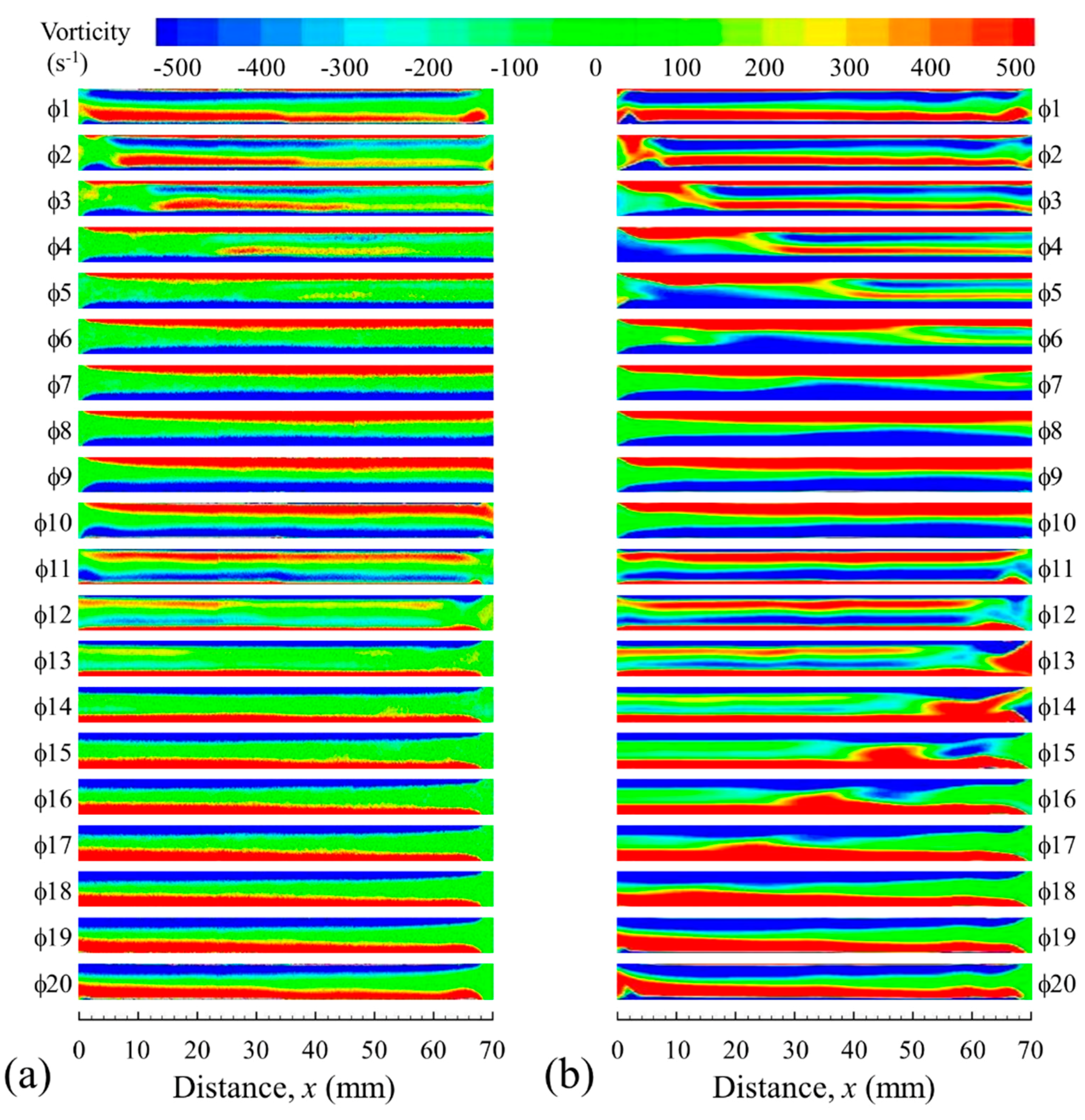
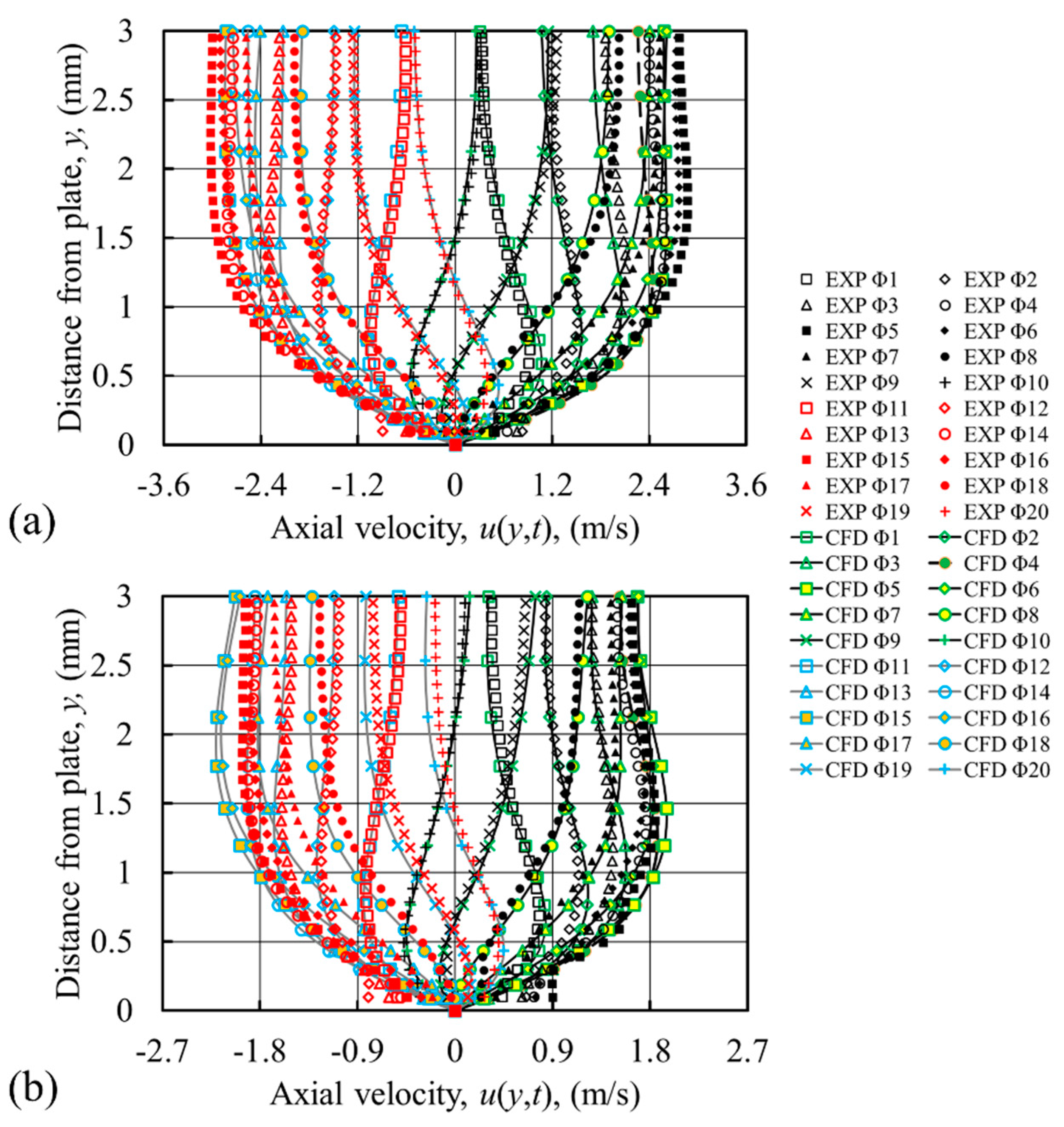
However, the centreline velocity alone is not sufficient to represent the flow, and therefore, the instantaneous velocity profiles across the channel need to be inspected. These are plotted in Figure 4 for the same axial location, from the wall surface () to the middle of the channel (), for all 20 phases of a flow cycle, separately for each drive ratio. Clearly, the already shown mismatch between the CFD and experimental magnitudes of axial velocity at y = 3 mm can be seen also in Figure 4, but more importantly, the whole profiles show substantial discrepancies at other locations, especially near the wall. The over-prediction of velocity profiles near the wall as calculated by the laminar model hints at the presence of turbulence [25].
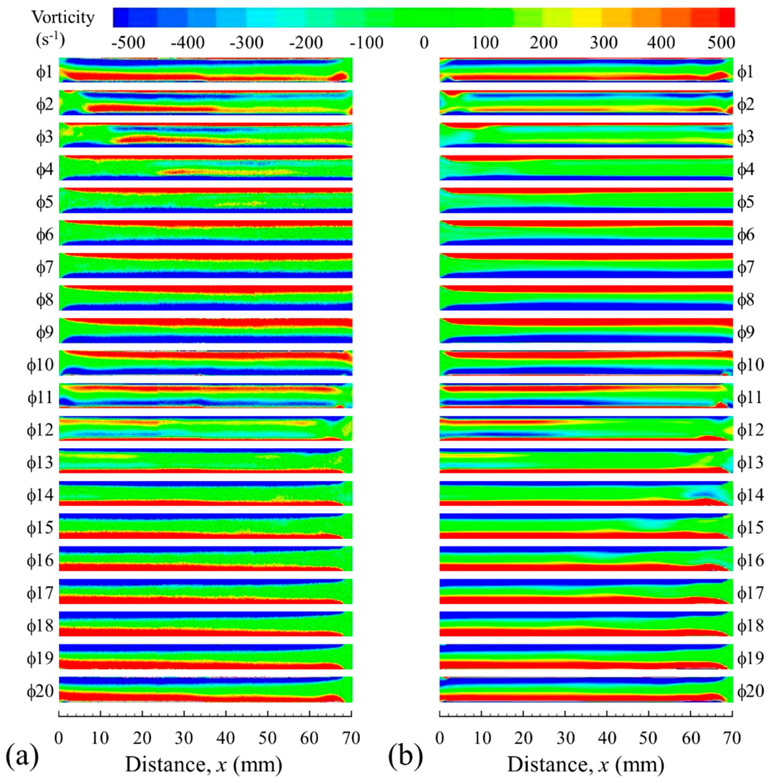
Furthermore, as the drive ratio increases, the discrepancies between velocity profiles from laminar CFD and experiments become larger, which indicates that the laminar model may not be sufficient to capture the flow behaviour. These discrepancies are also illustrated in Figure 5 as a vorticity contour map (drive ratio 0.83% selected as an example), which covers the area of the hot and cold channel. The numerical solutions appear to indicate the presence of very strong elongated secondary vortices (also referred to as a secondary shear layer), which are much less intense in reality, the best examples of such discrepancies being shown for 3. Furthermore, the laminar model also produces “blobs” of vorticity that travel within the channel between phases 13 and 17, and this also has no match in the experimental results.
Many investigations (cf. [4,5]) have shown that oscillatory flow past parallel plate structures creates strong vortex structures at the end of plates. The remains of these structures tend to be re-entrained into the channel as the flow changes direction. This suggests that there may be sufficient instabilities present in the flow to trigger turbulent transition. Furthermore, the critical Reynolds number defined in [7] was strictly for a flow within a long, ideally infinite, channel. Therefore, it is possible that transition may be triggered at much lower for flows past short plates. This is why a range of turbulent models has been tested as presented in the next section.
3.2. Turbulent Flow Models
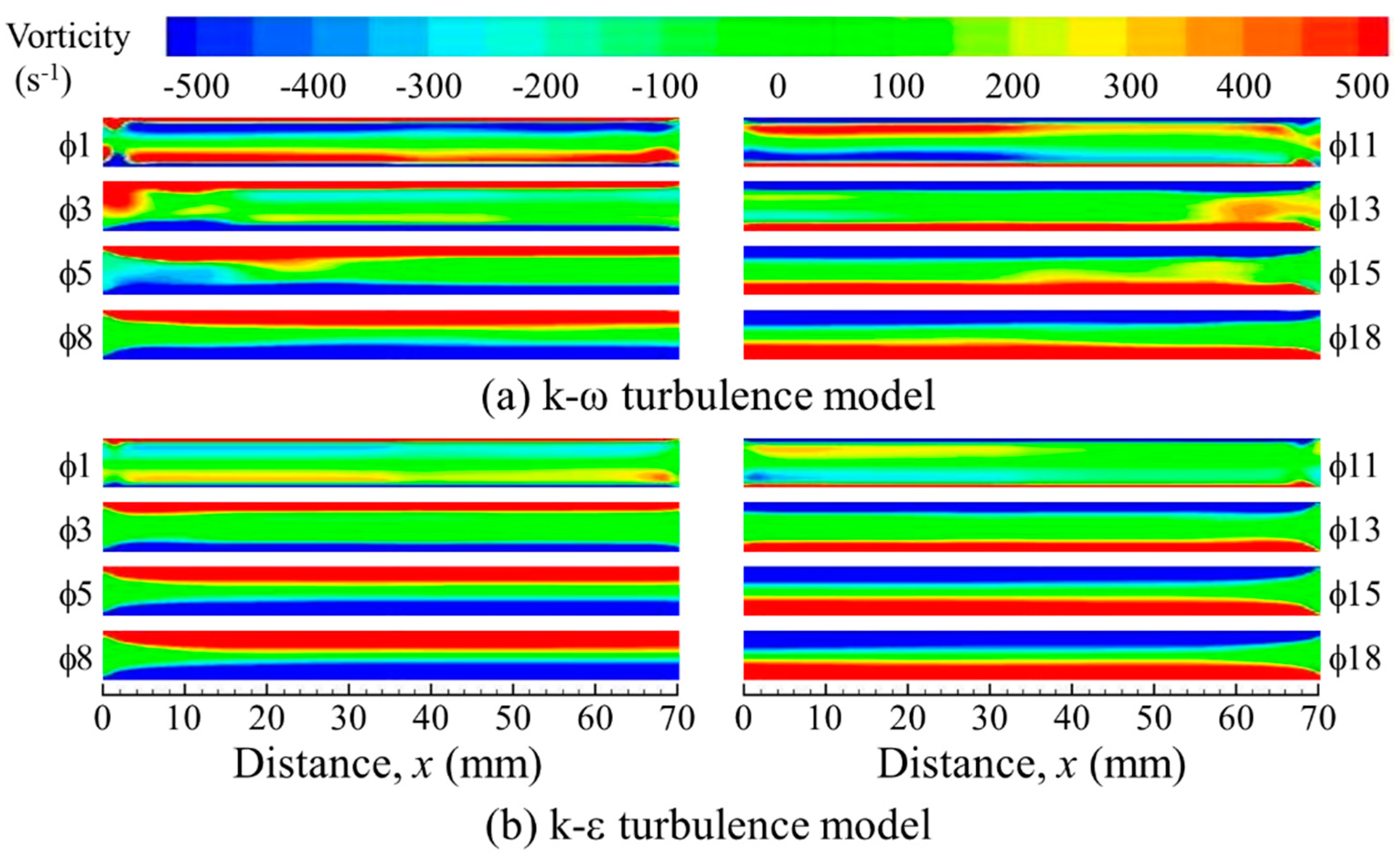
Figure 6 shows the vorticity contours for drive ratio of 0.83% obtained using two turbulence models: k-ω and k-ε. These are best discussed in comparison with Figure 5. The vorticity between the plates predicted by the k-ω model exhibits weaker vortex structures compared to the results obtained from the laminar model. However, there is still a suspect “blob” of vorticity that travels within the channel that is not seen in the experiment. On the other hand, the k-ε model produces much more realistic vorticity contours. However, when comparing experimental and CFD results for phases 1, 3, 11 and 13 in Figure 5a and Figure 6b, it is clear that the secondary shear layer (closer to the centre of the channel) is rather under-predicted by the CFD model. The results in Figure 5 and Figure 6 suggest that the disturbances leading to the creation of the elongated vorticity regions referred to as secondary shear layers and the “blobs” of vorticity described above originate from the open area at the end of plates.
Therefore, a further investigation into the vortex structures at the end of the plates was conducted to help choose turbulence models that best describe the flow, as illustrated in Figure 7, Figure 8 and Figure 9. Figure 7, based on experimental results at drive ratio 0.83%, shows that the flow enters the left end of the heat exchanger assembly at phase 1 and reaches the maximum amplitude at 5. During these phases, a weak vortex structure from the open area next to the left end of the HHX moves into the channel. The vortex structure at the right end of the heat exchanger assembly elongates as the velocity increases, but stays attached to the plate ends until the maximum velocity is reached at 5. When the flow decelerates, the vortex structures at the right end of the plates start shedding, as seen at 8. Similar behaviour is observed for the second half of the cycle as the flow reverses (phases 11 to 20), although differences in the flow patterns exist due to the asymmetry of the temperature profile (cf. Figure 2).
Figure 8 shows vorticity contours at the ends of the heat exchanger assembly for drive ratio of 0.83% calculated using the k-ε model. The vortex pattern is very different form the experimental one: vortex structures at the right end of the plate for 3 appear more stable. The pair of vortex structures at the end of plates elongates until the flow reaches maximum velocity at 5. In the experiment, vortex structures start to “wiggle” in this phase, which the k-ε model does not seem to predict.
As the flow decelerates, the elongated structures predicted by the k-ε model retain their shapes, but start to lose their strength, which reduces considerably by the time the flow reverses at 11. The weak vortex structures are re-entrained by the channel flow to create the elongated secondary vortex structures (secondary shear layers). In the second half of the cycle, similar stable vortex structures are observed on the left end of the plates. Importantly, the discrete vortex shedding phenomena are not seen in the results obtained from the k-ε turbulence model.
Figure 9 shows vorticity contours at the left and right ends of the heat exchanger assembly calculated for the drive ratio of 0.83% using the k-ω model. The vortex structures have a closer resemblance to the experimental result than those from the k-ε model. The vortex shedding process starts at the right end at 1 and the left end at 11. The vortex strengths seem slightly over-predicted, compared to the corresponding structures that appear somewhat weaker in the experimental results. The differences may be related to the consequence of “stitching” and “averaging” of the experimental results as explained in the original papers by Shi et al. [17] and Mao and Jaworski [4]. It may also be the result of two-dimensional assumptions used in the current turbulence model. Nevertheless, the resemblance of the flow structures to the experimental ones is quite convincing.
The results show that the flow structures at the end of the plates are best predicted by the k-ω turbulence model. The slight disparity with experimental results observed for the vorticity plots within the area bounded by the plates of the heat exchangers may require a more refined investigation. Menter [26] proposed a modified two-equation model called the shear-stress-transport (SST) k-ω model. It was proposed based on the observations of the performance of the conventional k-ε and k-ω models; the k-ε model is reported to perform best in the wake and free stream region while the k-ω model performs best for flows in bounded areas. Therefore, SST k-ω model uses both the k-ε and k-ω models appropriately, based on a control parameter that applies the correct model depending on the distance to the nearest wall. The model is suggested to cater for flows that involve both inviscid and viscous regions. It was used in this study to obtain better predictions and was first tested for the highest drive ratio of 0.83%.
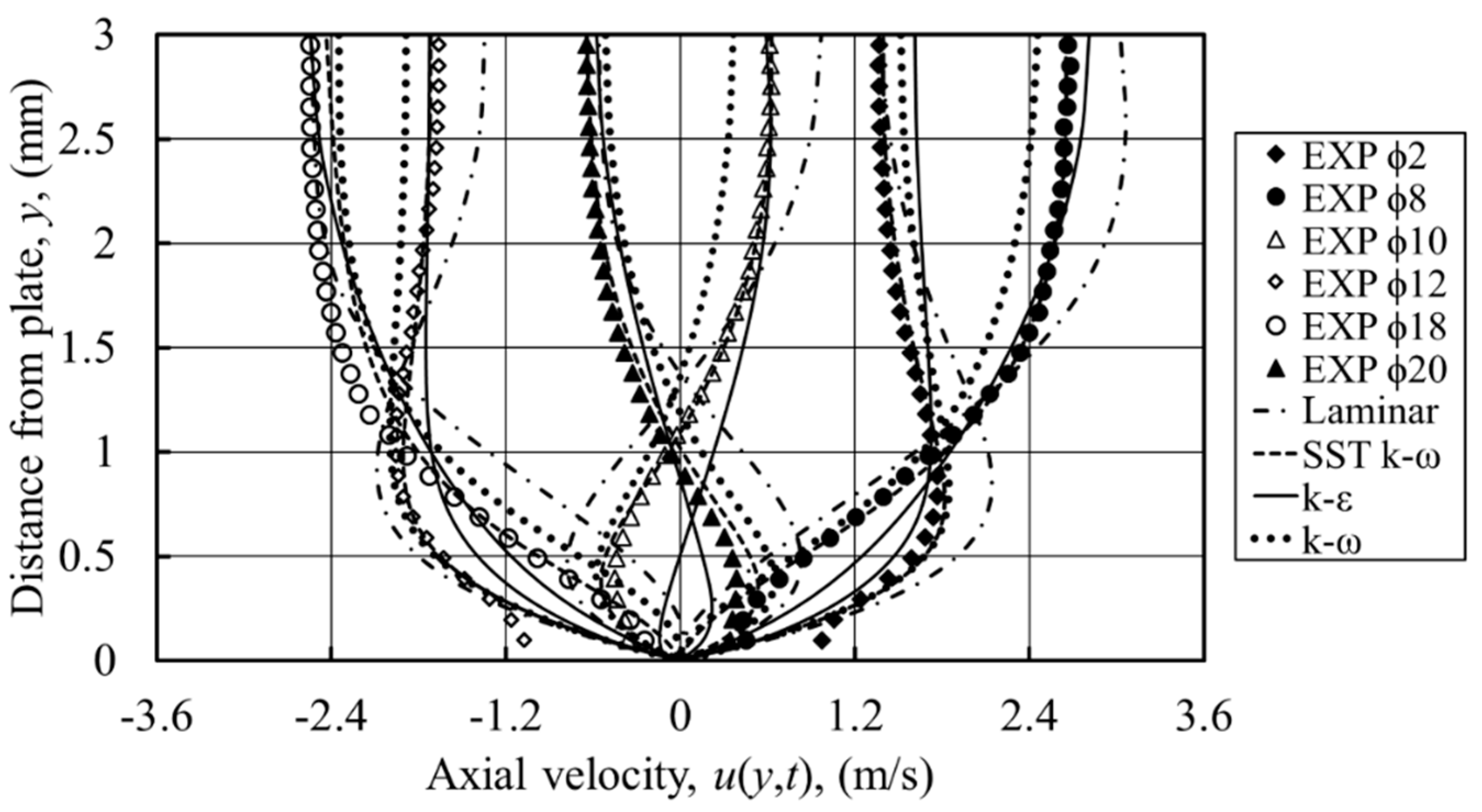
The comparison between velocity profiles from the experimental results and the numerical models tested is shown in Figure 10 for selected phases of the flow cycle at the drive ratio of 0.83%. They are plotted at the location 10 mm away from the joint, above the cold plate. As mentioned earlier, the laminar model over-predicts the profiles especially at locations near the wall. The predictions from the k-ε and k-ω models miscalculate the magnitude of velocity both near the wall and within the flow “core” away from the wall. Taking 10 as an example, the k-ε model gives good predictions at the core, but under-predicts the velocity magnitude near the wall. On the other hand, the k-ω model gives a better prediction near the wall, but under-predicts the magnitude of the velocity at the core. The profiles are better predicted by the SST k-ω model.
Figure 11 presents a comparison between experimental and numerical results from the SST k-ω model for all 20 phases. A good match, with a maximum error of 4.3%, is found for almost all phases in the flow cycle. Figure 12 gives a similar comparison in terms of vorticity contours: a very good qualitative match is found. A slight disagreement on the strength of the secondary shear layer is still visible during the first few phases that represent the acceleration stages of a flow cycle (2 to 4 and to ). This may be related to the uncertainty of the measurement, as well as the two-dimensional assumptions of the numerical model used in a three-dimensional situation. Nevertheless, the SST k-ω model has provided the best solution for the drive ratio of 0.83% with the closest match to the experiment.
The vorticity contours at the ends of the heat exchanger assembly, calculated using the SST k-ω model, are shown in Figure 13. They agree well with the experiment and are similar to the results from the k-ω model. This indicates that the vortex structures at the end of the plates are strongly influenced by the processes in the shear layer near the wall of the channel and that a correctly-defined flow condition within the channel leads to a better prediction of flow structures at the end of the plate. Clearly, the SST k-ω model with its excellent control parameter has given an improved prediction in both areas of the flow field.
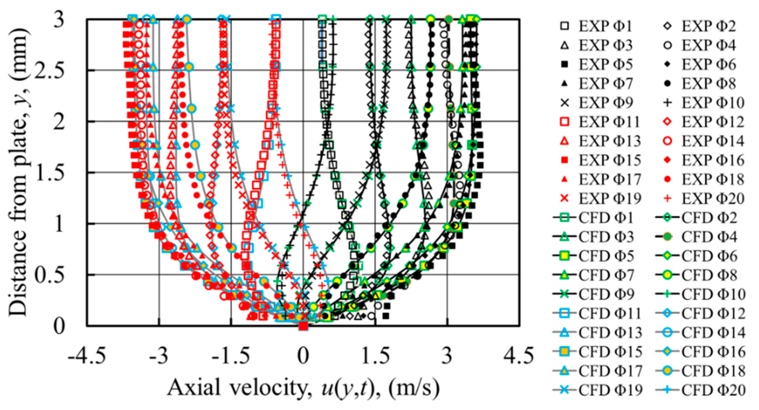
Following the successful application of the SST k-ω model at the drive ratio of 0.83%, it was subsequently applied to the other two drive ratios of 0.45% and 0.65%. The resulting velocity profiles for all 20 phases, together with experimental data, are shown in Figure 14. For the drive ratio of 0.65%, a better match to the experiment is obtained, compared to laminar predictions shown earlier in Figure 4c. The maximum deviation in Figure 4c occurs at 5, where the velocity was numerically over-predicted by 8.9%. With the SST k-ω model, the maximum deviation is slightly reduced to 8.3%. The match is not as good as predicted for the drive ratio of 0.83%. For the drive ratio 0.45%, the SST k-ω model provides no improvement in the velocity profiles compared to the laminar model. This may indicate that the flow at the drive ratio of 0.45% has not yet reached a state suitable for the application of a turbulence model. However, the laminar model does not provide a satisfactory solution either.
Observations of the experimental and numerical results in two extreme conditions of drive ratios of 0.3% and 0.83% suggest the occurrence of transition within this range. Therefore, the four-equation transition model (transition-SST [27]) is used. Figure 15 shows the resulting velocity profiles for drive ratios of 0.45% and 0.65%. The velocity profiles for a drive ratio of 0.65% are slightly better predicted than the profile shown in Figure 14a, with the maximum error of 5.3%. Hence, the transition model seems to be a better model for predicting the flow at this drive ratio. The difference in amplitude of velocity between experimental and numerical results at 5 and 15 may be due to the moderation constant [21,23,26,27] not being varied in this study.
For drive ratio of 0.45%, the transition-SST model provides velocity profiles that agree well with the experiment, with the maximum deviation of 5.2% (cf. Figure 15b). This may indicate that the flow at this drive ratio is already transitional in its nature. Generally, in oscillatory flow, turbulent transition is a much more complex process than in uni-directional flow. Swift [1] summarizes that the transitional region exists between the “weakly turbulent region” (flow with turbulent bursts at the centre of the pipe with the boundary layer remaining laminar) and the “conditionally turbulent region” (where the flow changes between “weakly turbulent” and “fully-turbulent” flow within a cycle). Furthermore, an oscillatory flow may also experience “relaminarization” where a “turbulent-like” flow is followed by a “laminar-like” flow in one cycle (cf. [8,9]).
As seen from Table 1, the drive ratios investigated here correspond to Stokes’ layer-based Reynolds number, , well below 400, which would be the critical Reynolds number for an infinite pipe [7]. However, the heat exchanger assembly in the current study has a short length. The disturbances from the edge of plates and the vortices shed and subsequently re-entrained (cf. Figure 13) may act as flow instabilities triggering turbulent transition. This may explain the need for the turbulence/transition model even though the Reynolds number is seemingly below the widely-accepted critical value.
As discussed above, with reference to Figure 3, the velocity amplitude at location is not a suitable benchmark to judge the quality of CFD against experimental results. On the other hand, judging the appropriateness of the models from vorticity maps may not be entirely objective. It is possible to introduce various “metrics” to judge the quality of CFD solutions; one of the simplest resembles the concept of the standard deviation. When considering -velocity profiles in the channel, at a selected axial location as an example, it can be defined as follows:
where and simply denote the discrete locations between the wall and channel centreline (here, the maximum is ) and the phase number in the cycle (here, the maximum is ), respectively. It attempts to describe the deviation of the CFD-based profile from the experimental profile, or in other words, the “goodness” of predictions. The numerical values are appropriately interpolated so that y-coordinates of CFD points match with the experimental ones. Of course, the smaller the metric , the better the match.
Figure 16 shows the plot of metric for the application of three models: laminar, transition-SST and SST k-ω at the drive ratios studied. It is clear that for the smallest drive ratio, all models give a very similar value of . As the drive ratio increases, the laminar model gives the largest discrepancies (the metric grows almost linearly). Meanwhile, the transition-SST model seems to give the best predictions for drive ratios of 0.45% and 0.65%, while SST k-ω gives the best prediction for the highest drive ratio of 0.83%. This is congruent with the previous discussions that identify the transition processes for drive ratios as low as 0.45%. Of course a caveat must be made that in this example, a selected profile of velocity at the location 10 mm away from the joint above the cold plate is considered.
The velocity magnitudes tabulated in Table 1 can also be used to represent the gas displacement, ; hence, the drive ratios of 0.30%, 0.45%, 0.65% and 0.83% correspond to the gas displacements of 16, 23, 36 and 47 mm, respectively. Clearly, the gas parcel in the flow with a drive ratio higher than 0.65% moves by a distance longer than half of the total length of the heat exchanger channel (70 mm). The forward and backward movements of the gas parcel convey the energy of the vortex structures at the end of plates into the channel.
Vortex structures of the selected phase, 8, obtained from the numerical calculations for drive ratios of 0.3% and 0.83% are shown in Figure 17. Evidently, the strong vortices appearing in the plate wake for the drive ratio of 0.83% can create strong flow disturbances when pushed back into the channel. This could be a possible explanation for the appearance of turbulence (and the need for transition/turbulence model) at this drive ratio as a means of dissipating the flow energy.
The growth of any flow disturbances that occur between the plates of the heat exchanger can also be complicated by the effects of the thermal expansion that causes the gas particles to move at a different displacement amplitude for the two halves of one cycle. The short length of the plates investigated in this study prohibits the flow of high drive ratios to reach a fully-developed state. Most heat exchangers are short, and a practical system works with a high drive ratio. This study suggests that turbulence is likely to occur within heat exchangers working in the oscillatory flow condition for Stokes Reynolds numbers well below the critical value of 400 given by Merkli and Thomann [7].
3.3. Viscous Dissipation
In a viscous flow, the energy of the fluid motion (kinetic energy) is turned into internal energy of the fluid through the existence of viscous dissipation. A dimensionless approach, introduced by Worlikar [11] and Mao [28], has been used with appropriate consideration of the porosity of the area within the heat exchanger and the open areas next to both ends of the heat exchanger (0.65 and one, respectively) [22]. The total dimensionless viscous dissipation is calculated as:
where:
The terms , and in Equation (15) are the area, viscosity and phase of a flow cycle, respectively; the term in square brackets is the area-weighted-average value of dimensionless dissipation, which is also averaged over one flow cycle. The dimensionless dissipation in Equation (16) is related to the mean flow velocity. The results in Figure 18 are shown as a product of porosity, , Eckert number, (where , and are the reference values of velocity, specific heat and temperature, respectively) and the area-weighted-average value of dimensionless dissipation. The reference values are taken at the location 200 mm away from the end of CHX. More detailed explanations and dimensional analysis were already given by Mohd Saat and Jaworski [21]. The Eckert number, , expresses the relationship between the flow kinetic energy and enthalpy and is used to characterise dissipation.
The viscous dissipation presented by Equation (16) is also known as “direct dissipation”, not to be confused with turbulent dissipation [25]. The velocity components and in Equation (16) are the mean velocity components of the flow. As with the laminar model, the direct dissipation represents the transfer of mechanical energy to internal energy through viscosity. The turbulent dissipation (which is the transfer of energy from the mean motion into the turbulence fluctuation and then into the internal energy) is indirectly affecting the mean flow when the turbulence model is used. The effect of turbulence on the internal energy of the flow is reflected in the final velocity of the mean flow used in Equations (1), (2) and (16). The laminar model was used for the drive ratio of 0.30%, the transition-SST model for drive ratios of 0.45% and 0.65%, while the SST k-ω model for the drive ratio of 0.83%.
Figure 18 shows that the viscous dissipation increases as the drive ratio increases. The increment occurs in areas both within the channel (Figure 18a) and the area outside (Figure 18b). Hot areas have a higher viscous dissipation compared to cold ones, due to the increase of viscosity with temperature. Furthermore, thermal expansion at the area bounded by the wall of the HHX and the buoyancy-driven flow as reported in [16], particularly prominent at the hot end, may well be responsible for the higher viscous dissipation within these areas. As the drive ratio increases, the amplitude of flow increases, and the viscous dissipation becomes larger.
3.4. Heat Transfer Condition
Finally, the wall heat transfer calculated from the CFD models is compared to the experimental data. Heat flux, , for all models is averaged over one cycle and the length of the heat exchanger, , and calculated as:
Subscripts and refer to HHX and CHX, respectively. Here, the mean thermal conductivity, , is used to calculate the heat flux obtained from laminar, transition-SST and SST k-ω models [22].
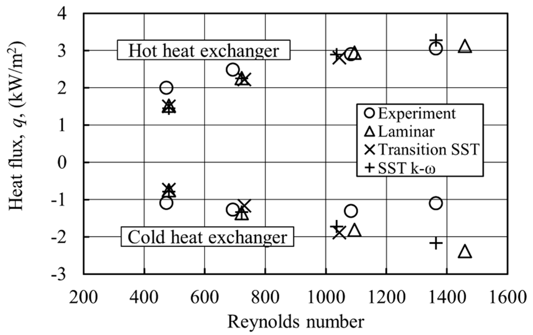
Figure 19 shows that the heat flux predicted from the numerical models and experiments increases with an increase of the drive ratio (indeed, for easier comparisons with the literature, the drive ratio is replaced by the Reynolds number, but it is still easy to identify the four drive ratios). The Reynolds number is calculated as as already outlined in Section 2. The flow behaviour for drive ratios investigated in this paper has been shown to be well predicted using the SST k-ω turbulence model and the transition-SST model. Therefore, the results shown in Figure 19 are based on the laminar and these two turbulent models.
In general, judging from Figure 19, the numerical predictions of heat transfer at the HHX are reasonably well aligned with the experimental values for all drive ratios. Here, the lowest discrepancy between numerical predictions and experiment is around 24% for the lowest drive ratio of 0.30%. As the drive ratio increases, the discrepancy drops to 7%. On the other hand, for the CHX, the agreement seems reasonable for the three lower drive ratios, 0.30%, 0.45% and 0.65%, where the lowest discrepancy is around 31%, 4% and 30%, respectively. The disagreement becomes substantially worse for the highest drive ratio of 0.83%, where the smallest discrepancy between CFD and the experiment is around 97%.
Of course, a judgement as to what constitutes reasonable agreement is somewhat arbitrary; however, the literature tends to agree that in complex flow cases like this, a discrepancy of around 30% is not unexpected. One also needs to remember that the experimental results were obtained from the acetone-based PLIF measurement technique with the stated temperature accuracy of ±16 K, where calibration for the low temperature end of the range is particularly challenging. This may well explain the discrepancies between CFD and experiment that tend to be within 30% in the majority of cases, but in particular, also the case of the highest drive ratio for the CHX, which seems to be an experimental “outlier”.
It is also worth comparing in detail the CFD results themselves. It is clear that the results obtained from the turbulent models are consistently closer to the experiment than from the laminar model (although this improvement is dwarfed by the overall large gap between all numerical results and the experiment). In particular, the transition-SST model gives better predictions of heat flux for drive ratios of 0.45% and 0.65% compared to predictions from the laminar model. For the highest drive ratio of 0.83%, the use of the SST k-ω, instead of the laminar, model brings the discrepancy of 117% down to 97%.
4. Conclusions
Numerical work presented in this paper builds upon previous experimental investigations [16,17] of the fluid flow and heat transfer processes in oscillatory flow conditions occurring at the coupled hot and cold plate-type heat exchangers. It presents a series of numerical studies, carried out using the ANSYS FLUENT 13.0 CFD package, aiming to match the experimental results by considering a range of flow models including laminar and four available RANS models: k-ε, k-ω, SST-k-ω and transition-SST. The key finding of this study is that in order to replicate the experimental flow fields, one would need to assume that the transition to turbulence occurs at much lower drive ratios than commonly accepted in the existing literature. In particular, the need for a turbulence model for the drive ratios as low as 0.45% has been demonstrated.
The investigation of the differences observed between the velocity profiles from the experiment and laminar model led to a hypothesis that turbulence may have influence on the flow, despite the commonly-accepted criterion for transition proposed by Merkli and Thomann [7]. This was concluded to be the effect of the finite length of the channel and the presence of the flow disturbances re-entrained after the vortex shedding cycle. Some validity to this description of the flow has been given by showing that the turbulent model gives a good match (with errors of ) between the results obtained from the experiment and the simulation, particularly at the drive ratio of 0.83% (the highest investigated). The SST k-ω model developed by Menter [26] is shown to best capture the essence of the flow at that drive ratio. The application of turbulence models makes the value of the metric , introduced to show the deviation between CFD and experimental velocity profiles, smaller. For instance, at the drive ratio of 0.83%, the metric value drops from 0.305 down to 0.174 as the SST k-ω replaces the laminar model.
It has been shown that transition may occur at a drive ratio as low as 0.45%, which translated into Stokes’ layer-based Reynold numbers corresponds to . The data shown in Table 1 would then in turn indicate the possible value of critical Reynolds number approximately within: 70 < Reδ < 100. This finding is important in that it contributes to a new understanding that the turbulent flow features may appear at lower flow amplitudes within structures of thermoacoustic systems. Of course, the nature of turbulence and transition in the oscillatory flows is not the same as in relatively better understood steady flows. It is known that there are quite a few different turbulent flow regimes in oscillatory flows, and these may appear at different parts of the cycle with a possibility of relaminarization. Therefore, in the context of the current study, it may well be necessary to refine any future CFD models from the point of view of the possible turbulence regimes in the oscillatory flows.
As expected, viscous dissipation increases with drive ratio. The dissipation is also higher within the hot areas. The results give an illustration of possible heat generation within certain areas of the thermoacoustic system as a result of dissipation. The amount of energy may not be large, but it may have a significant impact on the performance of fluid flow and heat transfer within small channels, such as those within the CHX and HHX. Since dissipation is very much related to the values of velocity, the correct prediction of velocity profiles, especially near the wall, is very important. The heat exchangers are normally placed within the most important parts of thermoacoustic devices. Therefore, any contribution to the energy loses is worth considering.
The current study included the calculation of cycle- and space-averaged heat fluxes on the CHX and HHX plates. It is clear that none of the models used could replicate the experimental results very closely, and the reason for this may well be the measurement errors embedded in the experimental method. However, the general trends of heat flux versus drive ratio (or Reynolds number) appear to be correct for both HHX and CHX plates. Out of eight experimental case studied, four seem to have discrepancies below 10%, three within 31% and one within 100% (possibly an experimental “outlier”). Importantly, the application of relevant turbulence or transition models in appropriate flow conditions tends to close the gap between the CFD and experimental results.
Acknowledgments
The first author would like to acknowledge the sponsorship of the Ministry of Education, Malaysia and Universiti Teknikal Malaysia Melaka (FRGS/1/2015/TK03/FKM/03/F00274). The second author would like to acknowledge the sponsorship of the Royal Society Industry Fellowship (2012–2015), Grant Number IF110094, and the EPSRC Advanced Research Fellowship, Grant GR/T04502.
Author Contributions
Fatimah A. Z. Mohd Saat performed the numerical investigations, analysed the data and drafted the paper. Artur J. Jaworski planned and supervised the research works, outlined the paper and subsequently worked with the first author on consecutive “iterations” of the paper till the final manuscript.
Conflicts of Interest
The authors declare no conflict of interest. The founding sponsors had no role in the design of the study; in the collection, analyses or interpretation of data; in the writing of the manuscript; nor in the decision to publish the results.
References
- Swift, G.W. Thermoacoustics: A Unifying Perspective for Some Engines and Refrigerators; Acoustical Society of America (through the American Institute of Physics): Melville, NY, USA, 2002. [Google Scholar]
- Zhang, S.; Wu, Z.H.; Zhao, R.D.; Yu, G.Y.; Dai, W.; Luo, E.C. Study on a basic unit of a double-acting thermoacoustic heat engine used dish solar power. Energy Convers. Manag. 2014, 85, 718–726. [Google Scholar] [CrossRef]
- Matveev, K.; Backhaus, S.; Swift, G. On Some Nonlinear Effects of Heat Transport in Thermal Buffer Tubes. In Proceedings of the 17th International Symposium on Nonlinear Acoustics, The Pennsylvania State University, PA, USA, 18–22 July 2006. [Google Scholar]
- Mao, X.; Jaworski, A.J. Application of particle image velocimetry measurement techniques to study turbulence characteristics of oscillatory flows around parallel-plate structures in thermoacoustic devices. Meas. Sci. Technol. 2010, 21. [Google Scholar] [CrossRef]
- Zhang, D.W.; He, Y.L.; Yang, W.W.; Gu, X.; Wang, Y.; Tao, W.Q. Experimental visualization and heat transfer analysis of the oscillatory flow in thermoacoustic stacks. Exp. Therm. Fluid Sci. 2013, 46, 221–231. [Google Scholar] [CrossRef]
- Ohmi, M.; Iguchi, M.; Kakehashi, K.; Masuda, T. Transition to turbulence and velocity distribution in an oscillating pipe flow. Bull. JSME 1982, 25, 365–371. [Google Scholar] [CrossRef]
- Merkli, P.; Thomann, H. Transition in oscillating pipe flow. J. Fluid Mech. 1975, 68, 567–575. [Google Scholar] [CrossRef]
- Akhavan, R.; Kamm, R.D.; Shapiro, A.H. An investigation of transition to turbulence in bounded oscillatory Stokes flows Part1. Experiments. J. Fluid Mech. 1991, 225, 395–422. [Google Scholar] [CrossRef]
- Narasimha, R.; Sreenivasan, K.R. Relaminarization of Fluid Flows. Advances in Applied Mechanics; Academic Press: Burlington, MA, USA, 1979; pp. 221–309. [Google Scholar]
- Arnott, W.P.; Bass, H.E.; Respet, R. General formulation of thermoacosutic for stacks having arbitrarily shaped pore cross sections. J. Acoust. Soc. Am. 1991, 90, 3228–3237. [Google Scholar] [CrossRef]
- Worlikar, A.S.; Knio, O.M. Numerical simulation of a thermoacoustic refrigerator I. Unsteady adiabatic flow around the stack. J. Comput. Phys. 1996, 127, 424–451. [Google Scholar] [CrossRef]
- Piccolo, A. Numerical computation for parallel plate thermoacoustic heat exchangers in standing wave oscillatory flow. Int. J. Heat Mass Transf. 2011, 54, 4518–4530. [Google Scholar] [CrossRef]
- Fieldman, D.; Wagner, C. On the influence of computational domain length on turbulence in oscillatory pipe flow. Int. J. Heat Fluid Flow 2016, 61, 229–244. [Google Scholar] [CrossRef]
- Abd El-Rahman, A.I.; Abdelfattah, W.A.; Fouad, M.A. A 3D investigation of thermoacoustic fields in a square stack. Int. J. Heat Mass Transf. 2017, 108, 292–300. [Google Scholar] [CrossRef]
- Sharify, E.M.; Takahashi, S.; Hasegawa, S. Development of a CFD model for simulation of a traveling-wave thermoacoustic engine using an impedance matching boundary condition. Appl. Therm. Eng. 2016, 107, 1026–1035. [Google Scholar] [CrossRef]
- Shi, L.; Mao, X.; Jaworski, A.J. Application of planar laser-induced fluorescence measurement techniques to study the heat transfer characteristics of parallel-plate heat exchangers in thermoacoustic devices. Meas. Sci. Technol. 2010, 21, 115405. [Google Scholar] [CrossRef]
- Shi, L.; Yu, Z.; Jaworski, A.J. Application of laser-based instrumentation for measurement of time-resolved temperature and velocity fields in the thermoacoustic system. Int. J. Therm. Sci. 2010, 49, 1688–1701. [Google Scholar] [CrossRef]
- Jaworski, A.J.; Piccolo, A. Heat transfer processes in parallel-plate heat exchangers of thermoacoustic devices-numerical and experimental approaches. Appl. Therm. Eng. 2012, 42, 145–153. [Google Scholar] [CrossRef]
- Rott, N. Thermoacoustics. Adv. Appl. Mech. 1980, 20, 135–175. [Google Scholar]
- Versteeg, H.K.; Malalasekera, W. An Introduction to Computational Fluid Dynamics the Finite Volume Method, 2nd ed.; Prentice Hall: Essex, UK, 2007. [Google Scholar]
- Mohd Saat, F.A.Z.; Jaworski, A.J. The effect of temperature field on low amplitude oscillatory flow within a parallel-plate heat exchanger in a standing wave thermoacoustic system. Appl. Sci. 2017, 7, 417. [Google Scholar] [CrossRef]
- Mohd Saat, F.A.Z. Numerical Investigations of Fluid Flow and Heat Transfer Processes in the Internal Structures of Thermoacoustic Devices. Ph.D. Thesis, University of Leicester, Leicester, UK, 2013. [Google Scholar]
- ANSYS FLUENT 13.0; User Manual, ANSYS Inc.: Canonsburg, PA, USA, 2010.
- Abramenko, T.N.; Aleinikova, V.I.; Golovicher, L.E.; Kuz’mina, N.E. Generalization of experimental data on thermal conductivity of nitrogen, oxygen, and air at atmospheric pressure. J. Eng. Phys. Thermophys. 1992, 63, 892–897. [Google Scholar] [CrossRef]
- Schlichting, H.; Gersten, K. Boundary Layer Theory, 8th revised and enlarged ed.; Springer: Berlin, Germany, 2001; pp. 76, 416–507. [Google Scholar]
- Menter, F.R. Two-equation eddy-viscosity turbulence models for engineering application. AIAA J. 1994, 32, 1598–1605. [Google Scholar] [CrossRef]
- Menter, F.R.; Langtry, R.; Volker, S. Transition modeling for general purpose CFD codes. Flow Turbul. Combust. 2006, 77, 277–303. [Google Scholar] [CrossRef]
- Mao, X.; Jaworski, A.J. Oscillatory flow at the end of parallel-plate stacks: Phenomenological and similarity analysis. Fluid Dyn. Res. 2010, 42, 055504. [Google Scholar] [CrossRef]
Figure 1.
A “short model” shown as a red-dashed box on the schematic diagram (top); computational domain (middle); and the area of the parallel-plate channel investigated (bottom).
Figure 1.
A “short model” shown as a red-dashed box on the schematic diagram (top); computational domain (middle); and the area of the parallel-plate channel investigated (bottom).
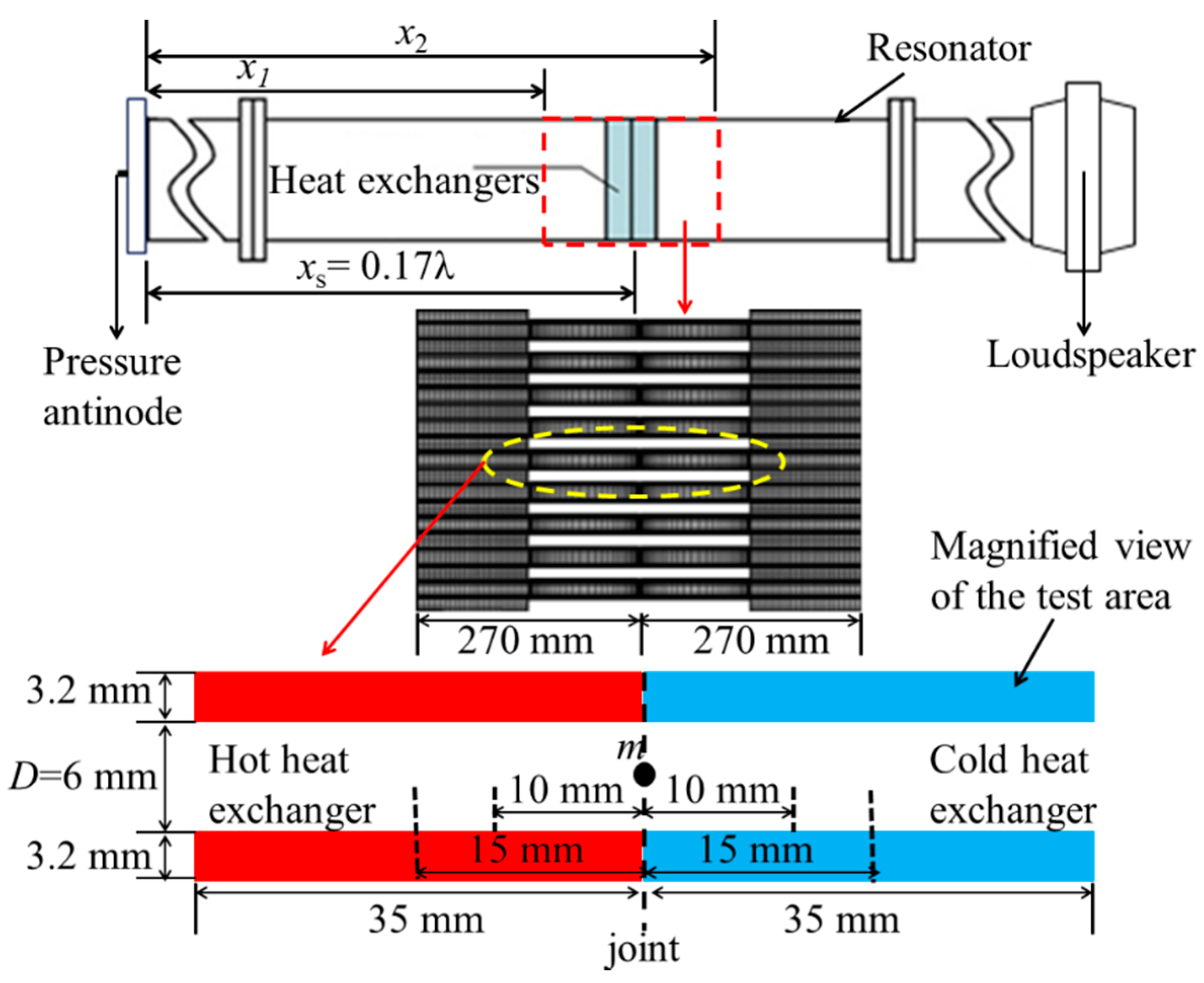
Figure 2.
Temperature profiles applied to cold and hot heat exchangers based on experimental points. CHX—cold heat exchanger; HHX—hot heat exchanger; CFD—computational fluid dynamics.
Figure 2.
Temperature profiles applied to cold and hot heat exchangers based on experimental points. CHX—cold heat exchanger; HHX—hot heat exchanger; CFD—computational fluid dynamics.

Figure 3.
Axial velocity in the middle of the channel at the location 10 mm away from the joint above the cold plate for drive ratios of (a) 0.30%, (b) 0.45%, (c) 0.65% and (d) 0.83%.
Figure 3.
Axial velocity in the middle of the channel at the location 10 mm away from the joint above the cold plate for drive ratios of (a) 0.30%, (b) 0.45%, (c) 0.65% and (d) 0.83%.
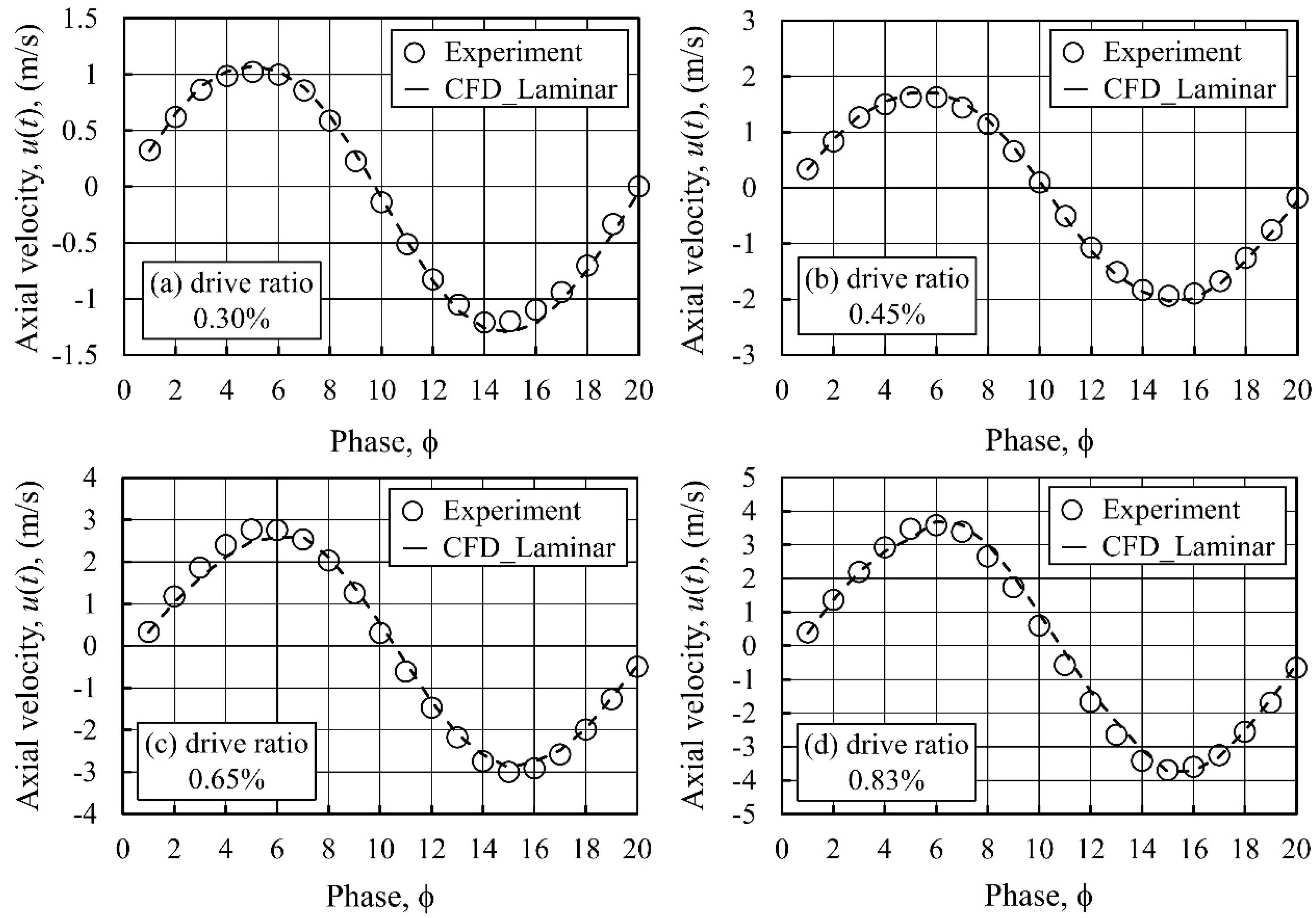
Figure 4.
Velocity profiles at location 10 mm away from the joint, within the cold channel, for drive ratio (Dr): (a) 0.30%, (b) 0.45%, (c) 0.65% and (d) 0.83%. Numerical results based on laminar model. EXP refers to experimental results.
Figure 4.
Velocity profiles at location 10 mm away from the joint, within the cold channel, for drive ratio (Dr): (a) 0.30%, (b) 0.45%, (c) 0.65% and (d) 0.83%. Numerical results based on laminar model. EXP refers to experimental results.

Figure 5.
Comparison between vorticity contour from (a) experiment and (b) CFD laminar model. The drive ratio is 0.83%. Distance x is measured from the left end of HHX/CHX assembly; vertical axis, is omitted for simplicity; the ratio of is 1:1.
Figure 5.
Comparison between vorticity contour from (a) experiment and (b) CFD laminar model. The drive ratio is 0.83%. Distance x is measured from the left end of HHX/CHX assembly; vertical axis, is omitted for simplicity; the ratio of is 1:1.

Figure 6.
Comparison between vorticity contours from the (a) k-ω and (b) k-ε turbulence models. The drive ratio is 0.83%. Distance is measured from the left end of HHX/CHX assembly; vertical axis, , is omitted for simplicity; the ratio of is 1:1.
Figure 6.
Comparison between vorticity contours from the (a) k-ω and (b) k-ε turbulence models. The drive ratio is 0.83%. Distance is measured from the left end of HHX/CHX assembly; vertical axis, , is omitted for simplicity; the ratio of is 1:1.

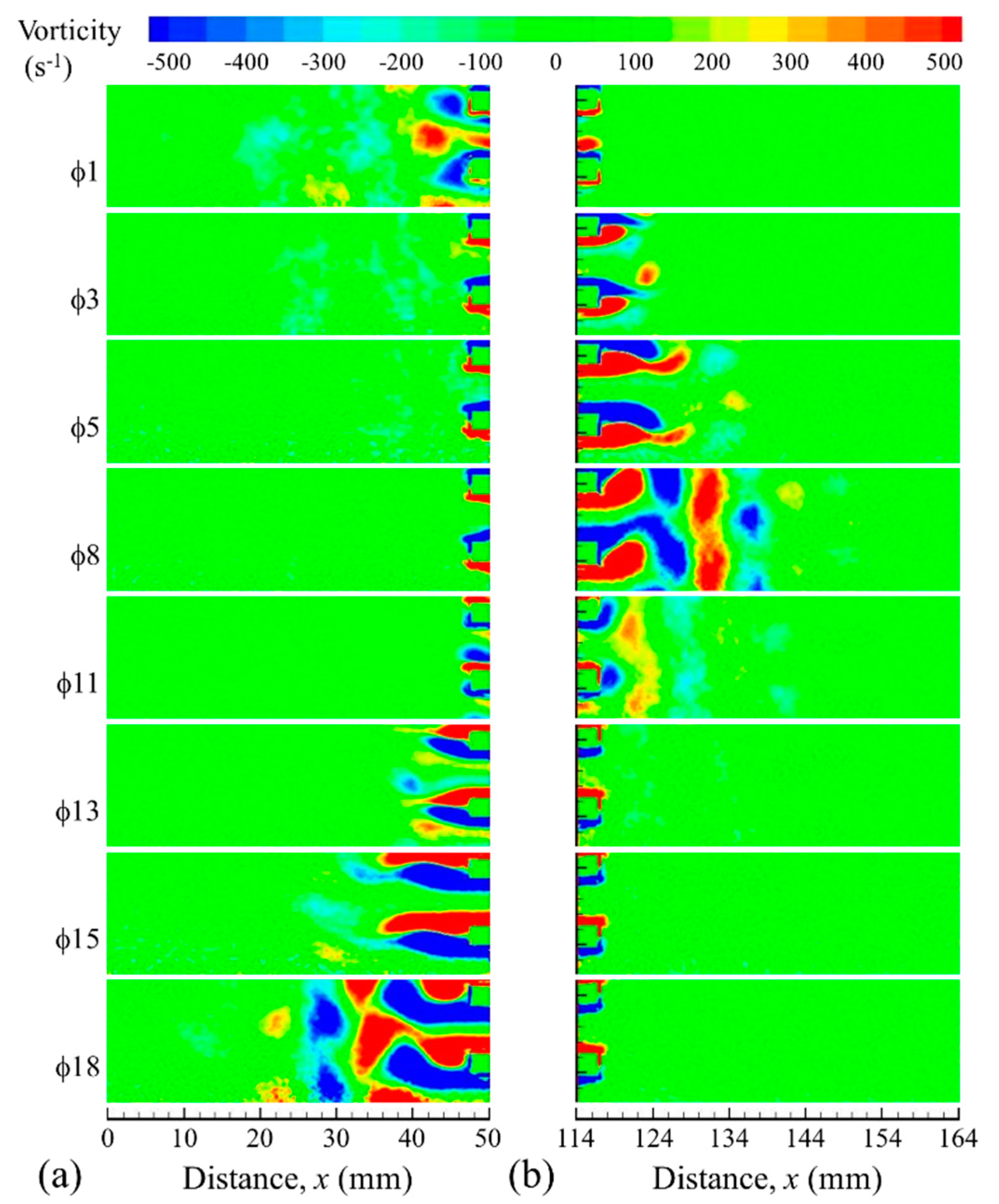
Figure 7.
Vorticity contours at the left (a) and right (b) ends of the heat exchanger assembly calculated from the experimental results for the drive ratio of 0.83%. Arbitrary distance is measured along the “viewing area”; vertical axis, , is omitted for simplicity; the ratio of is 1:1.
Figure 7.
Vorticity contours at the left (a) and right (b) ends of the heat exchanger assembly calculated from the experimental results for the drive ratio of 0.83%. Arbitrary distance is measured along the “viewing area”; vertical axis, , is omitted for simplicity; the ratio of is 1:1.

Figure 8.
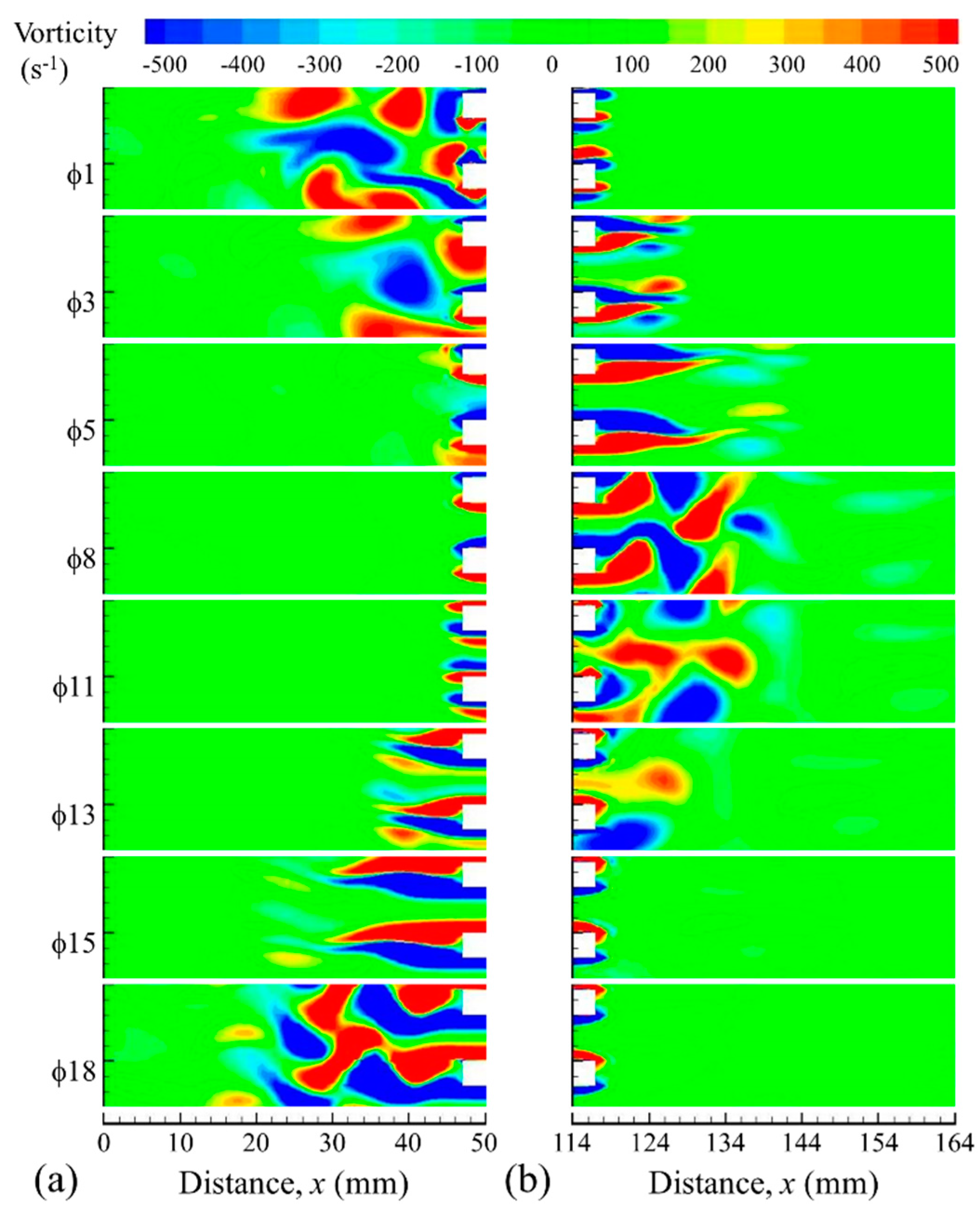
Vorticity contours at the left (a) and right (b) ends of the heat exchanger assembly calculated using the k-ε model for the drive ratio of 0.83%. Arbitrary distance is measured along the “viewing area”; vertical axis, , is omitted for simplicity; the ratio of is 1:1.
Figure 8.
Vorticity contours at the left (a) and right (b) ends of the heat exchanger assembly calculated using the k-ε model for the drive ratio of 0.83%. Arbitrary distance is measured along the “viewing area”; vertical axis, , is omitted for simplicity; the ratio of is 1:1.
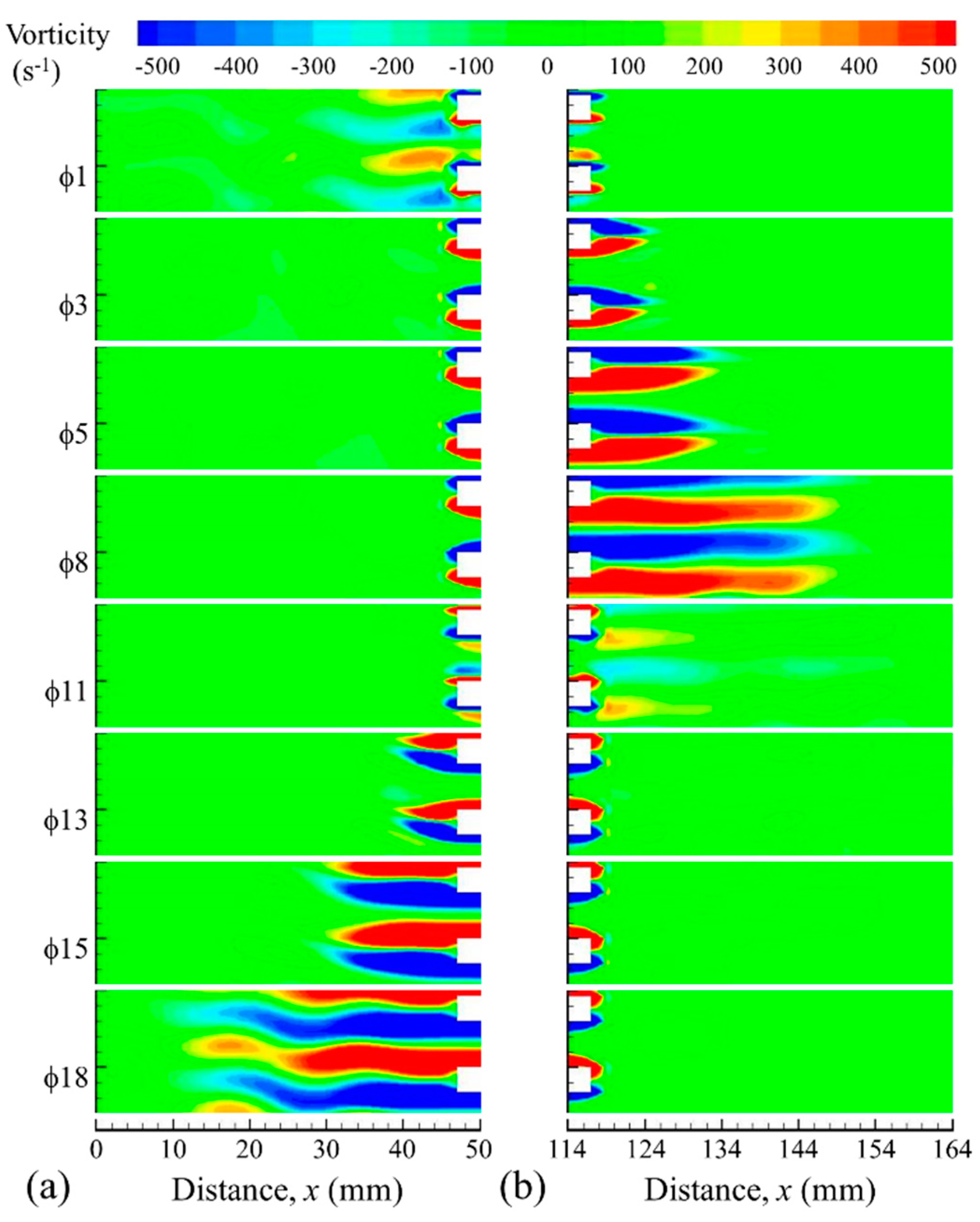
Figure 9.
Vorticity contours at the left (a) and right (b) ends of the heat exchanger assembly calculated using the k-ω model for the drive ratio of 0.83%. Arbitrary distance , is measured along the “viewing area”; vertical axis, , is omitted for simplicity; the ratio of is 1:1.
Figure 9.
Vorticity contours at the left (a) and right (b) ends of the heat exchanger assembly calculated using the k-ω model for the drive ratio of 0.83%. Arbitrary distance , is measured along the “viewing area”; vertical axis, , is omitted for simplicity; the ratio of is 1:1.

Figure 10.
Comparison between velocity profiles from experiments and CFD for the location 10 mm from the joint, in the cold channel, for the drive ratio of 0.83%. SST stands for shear-stress-transport.
Figure 10.
Comparison between velocity profiles from experiments and CFD for the location 10 mm from the joint, in the cold channel, for the drive ratio of 0.83%. SST stands for shear-stress-transport.

Figure 11.
Velocity profiles from the SST k-ω model (black and grey lines) and experiment (red and black symbols). Plotted for the location 10 mm from the joint, inside the cold channel, for the 0.83% drive ratio.
Figure 11.
Velocity profiles from the SST k-ω model (black and grey lines) and experiment (red and black symbols). Plotted for the location 10 mm from the joint, inside the cold channel, for the 0.83% drive ratio.

Figure 12.
Comparison between vorticity contours from the experiment (a) and the SST k-ω model (b). The drive ratio is 0.83%. Distance x is measured from the left end of HHX/CHX assembly; vertical axis, y, is omitted for simplicity; the ratio of x:y is 1:1.
Figure 12.
Comparison between vorticity contours from the experiment (a) and the SST k-ω model (b). The drive ratio is 0.83%. Distance x is measured from the left end of HHX/CHX assembly; vertical axis, y, is omitted for simplicity; the ratio of x:y is 1:1.

Figure 13.
Vorticity contours at the left (a) and right (b) ends of heat exchanger assembly calculated from the SST k-ω model. The drive ratio is 0.83%. Arbitrary distance x is measured along the “viewing area”; vertical axis, y, is omitted for simplicity; the ratio of x:y is 1:1.
Figure 13.
Vorticity contours at the left (a) and right (b) ends of heat exchanger assembly calculated from the SST k-ω model. The drive ratio is 0.83%. Arbitrary distance x is measured along the “viewing area”; vertical axis, y, is omitted for simplicity; the ratio of x:y is 1:1.
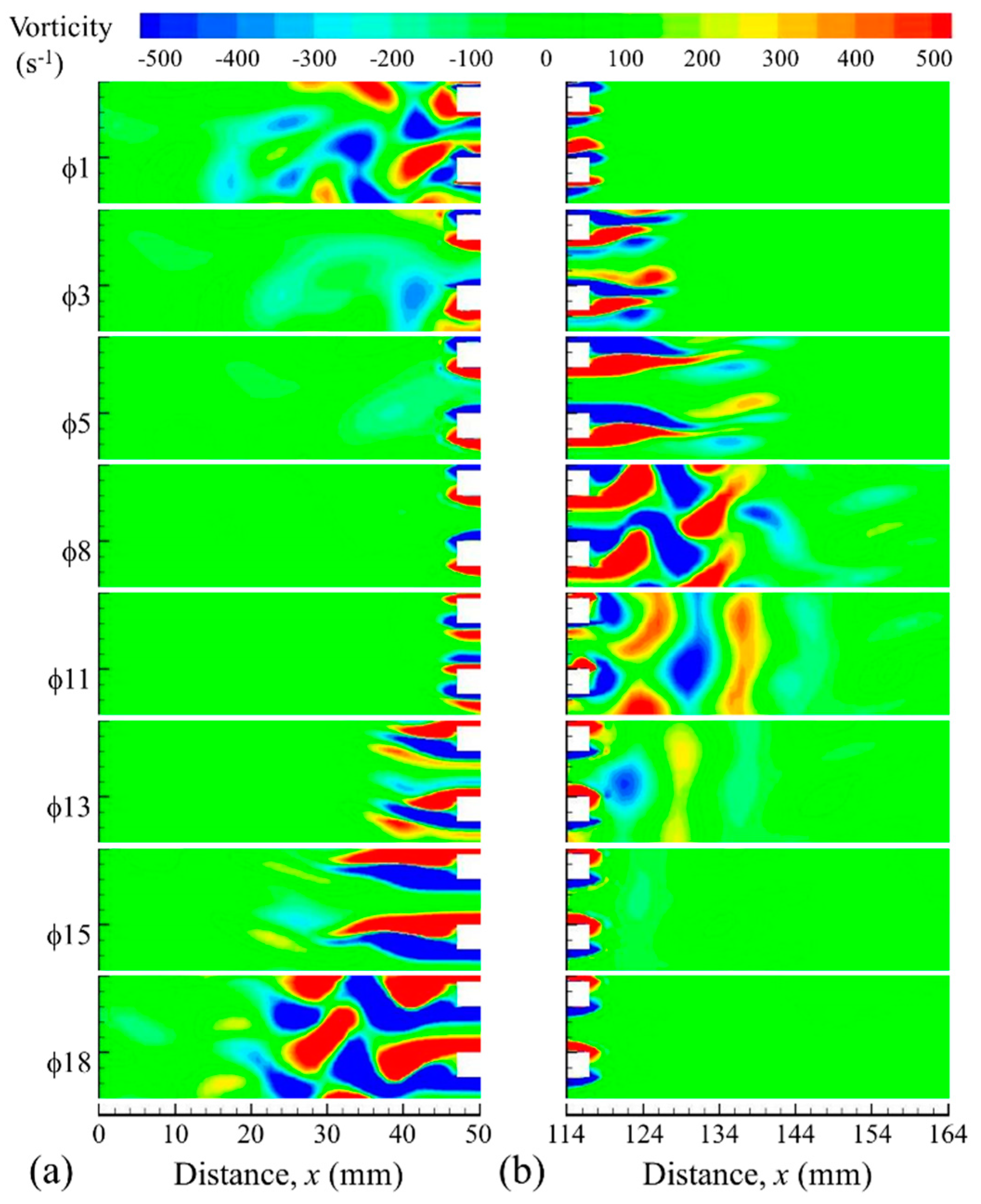
Figure 14.
Comparison between velocity profiles from the experiment and the SST k-ω model; for drive ratio of (a) 0.65% and (b) 0.45%. Location 10 mm from the joint inside the cold channel.
Figure 14.
Comparison between velocity profiles from the experiment and the SST k-ω model; for drive ratio of (a) 0.65% and (b) 0.45%. Location 10 mm from the joint inside the cold channel.

Figure 15.
Comparison between velocity profiles from the experiment and the transition-SST model for drive ratio of (a) 0.65% and (b) 0.45%. Location 10 mm from the joint inside the cold channel.
Figure 15.
Comparison between velocity profiles from the experiment and the transition-SST model for drive ratio of (a) 0.65% and (b) 0.45%. Location 10 mm from the joint inside the cold channel.
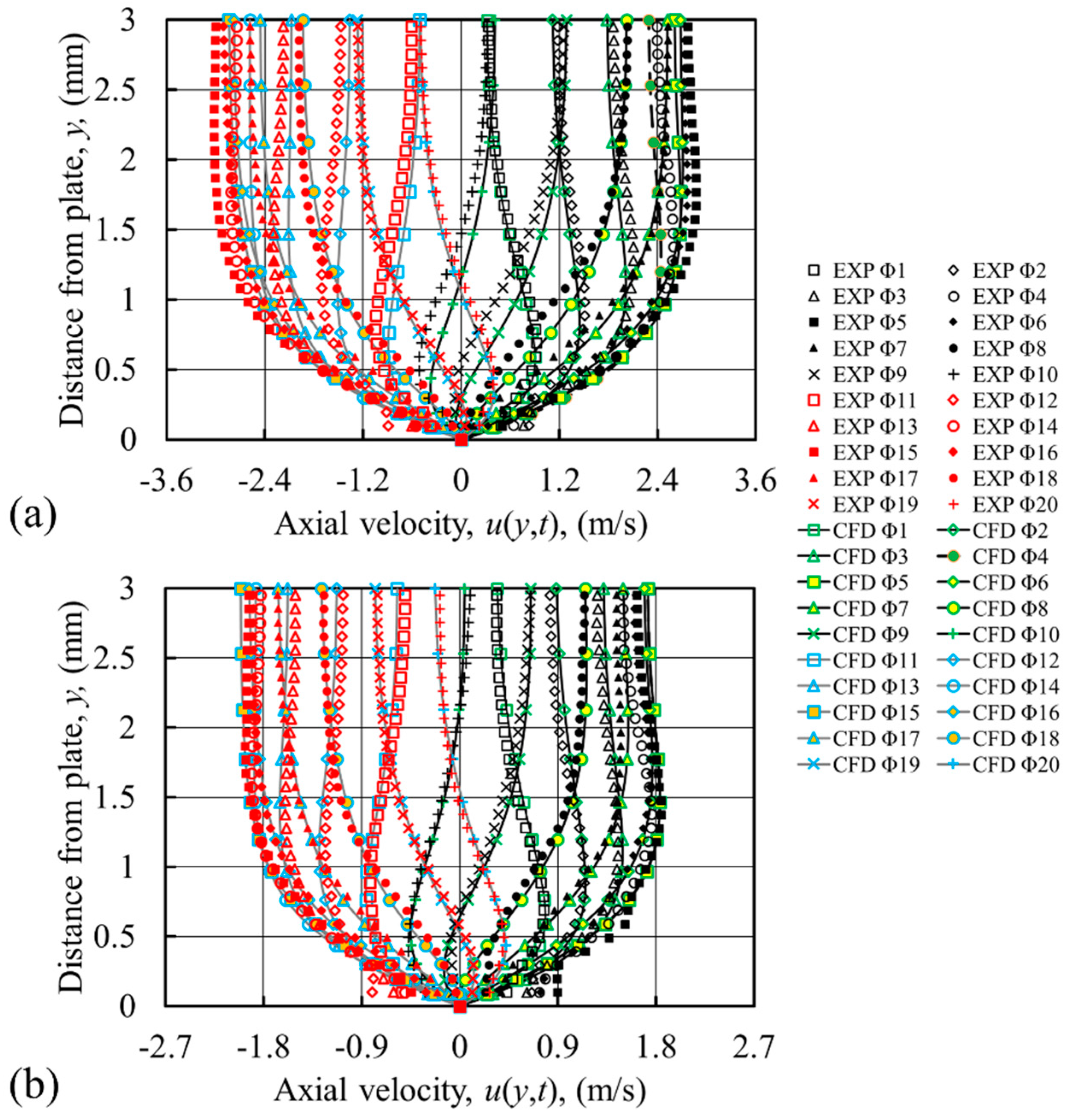
Figure 16.
Plot of metric for laminar, transition-SST and SST k-ω models vs. the drive ratio.
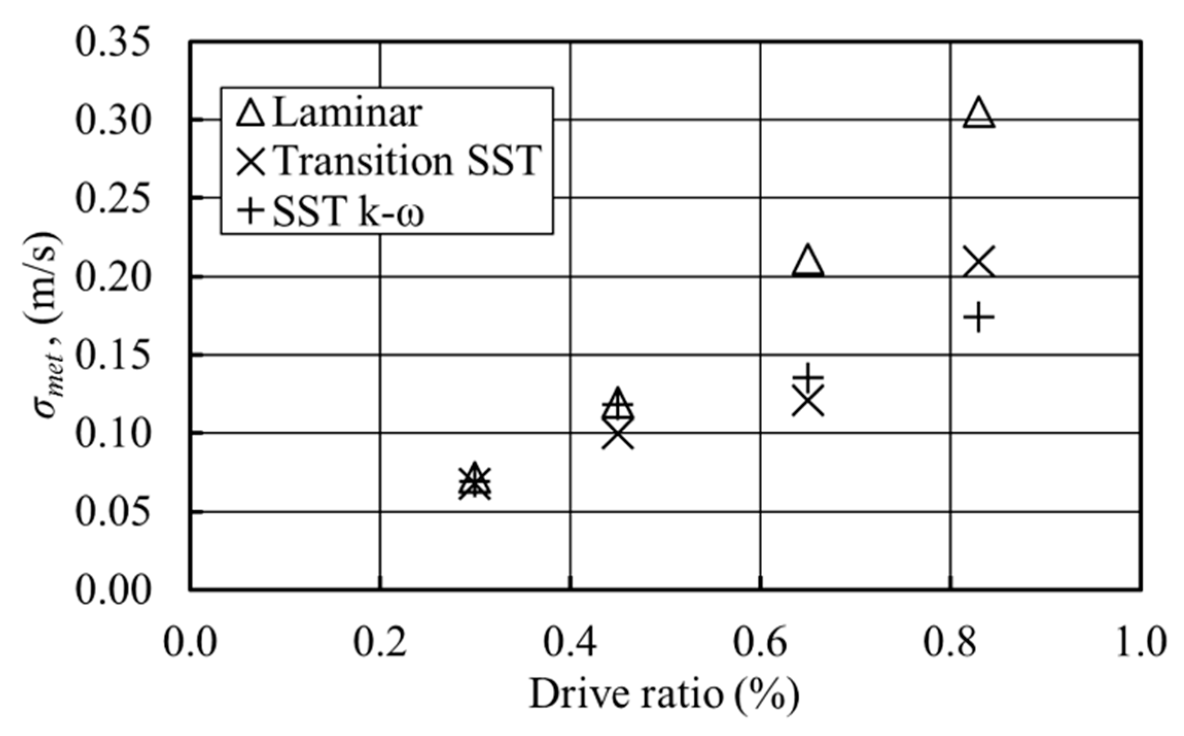
Figure 17.
CFD predictions of vorticity contours at the end of the cold heat exchanger for phase 8 at drive ratios of (a) 0.3% using the laminar model and (b) 0.83% using the SST k-ω model. Distances and measured from an arbitrary origin.
Figure 17.
CFD predictions of vorticity contours at the end of the cold heat exchanger for phase 8 at drive ratios of (a) 0.3% using the laminar model and (b) 0.83% using the SST k-ω model. Distances and measured from an arbitrary origin.
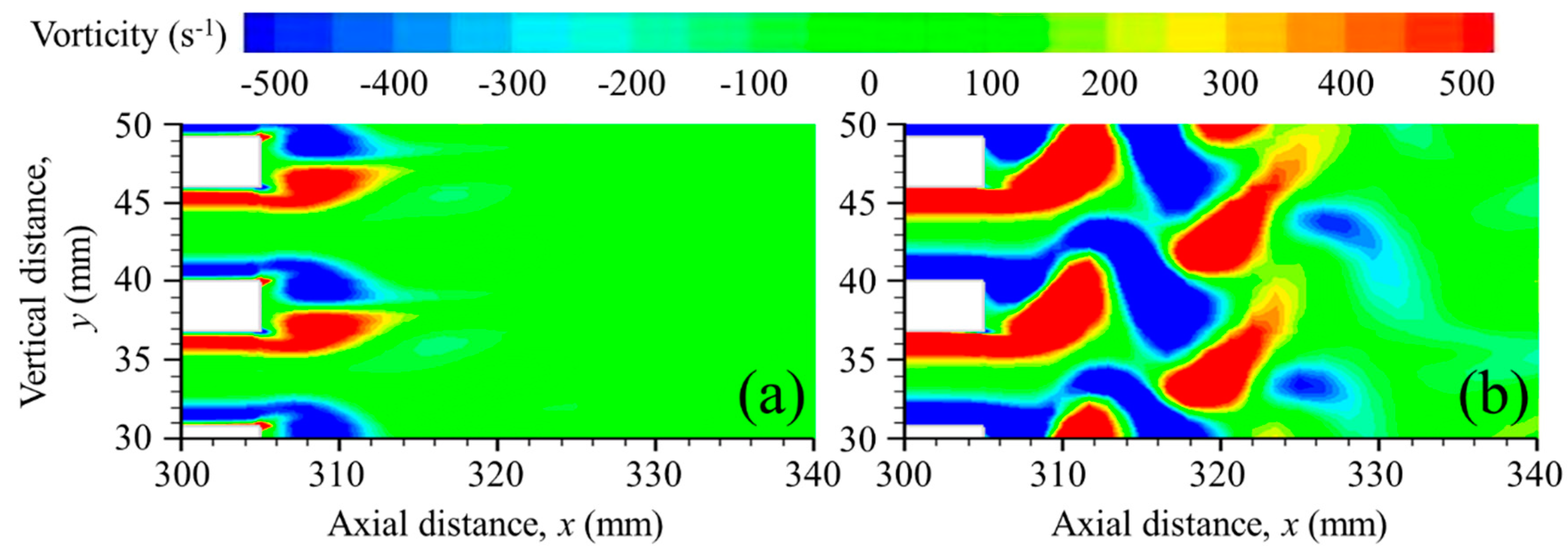
Figure 18.
The effect of the drive ratio on dimensionless mean flow viscous dissipation (a) and the enlarged view of the viscous dissipation at the end of plates (b).
Figure 18.
The effect of the drive ratio on dimensionless mean flow viscous dissipation (a) and the enlarged view of the viscous dissipation at the end of plates (b).
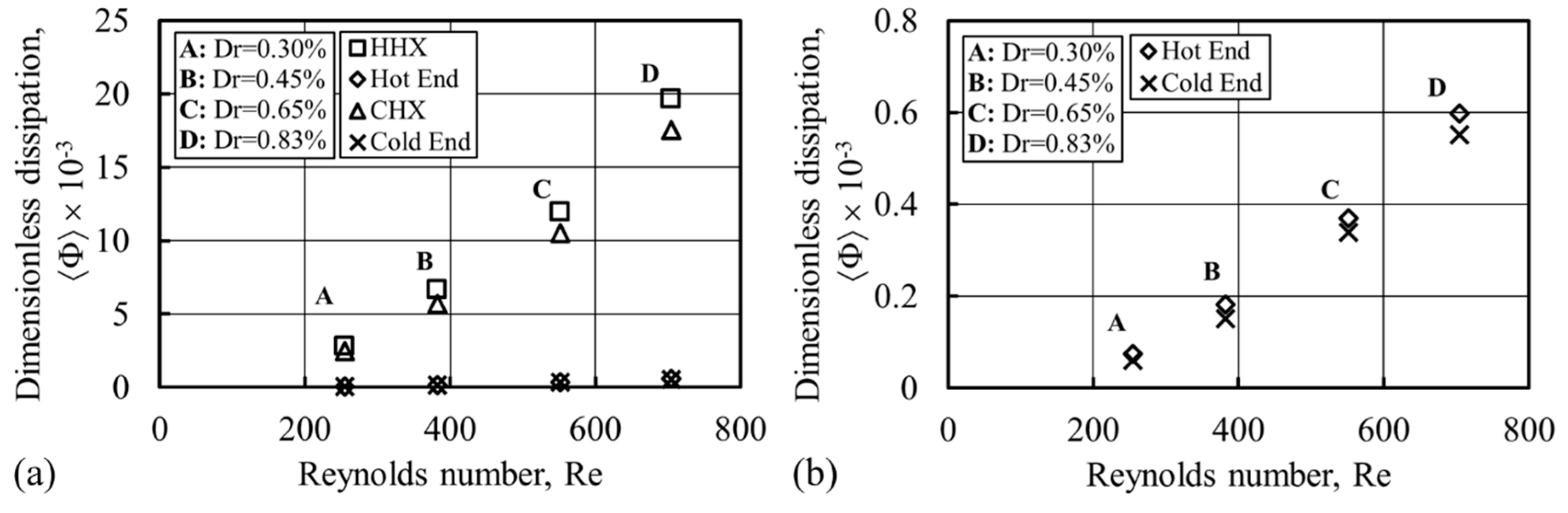
Figure 19.
Heat fluxes at cold and hot heat exchangers: comparison between numerical and experimental results.
Figure 19.
Heat fluxes at cold and hot heat exchangers: comparison between numerical and experimental results.


© 2017 by the authors. Licensee MDPI, Basel, Switzerland. This article is an open access article distributed under the terms and conditions of the Creative Commons Attribution (CC BY) license (http://creativecommons.org/licenses/by/4.0/).
Share and Cite
MDPI and ACS Style
Mohd Saat, F.A.Z.; Jaworski, A.J. Numerical Predictions of Early Stage Turbulence in Oscillatory Flow across Parallel-Plate Heat Exchangers of a Thermoacoustic System. Appl. Sci. 2017, 7, 673. https://doi.org/10.3390/app7070673
AMA Style
Mohd Saat FAZ, Jaworski AJ. Numerical Predictions of Early Stage Turbulence in Oscillatory Flow across Parallel-Plate Heat Exchangers of a Thermoacoustic System. Applied Sciences. 2017; 7(7):673. https://doi.org/10.3390/app7070673
Chicago/Turabian StyleMohd Saat, Fatimah A. Z., and Artur J. Jaworski. 2017. "Numerical Predictions of Early Stage Turbulence in Oscillatory Flow across Parallel-Plate Heat Exchangers of a Thermoacoustic System" Applied Sciences 7, no. 7: 673. https://doi.org/10.3390/app7070673
Note that from the first issue of 2016, this journal uses article numbers instead of page numbers. See further details here.