
Bonded-Particle Model with Nonlinear Elastic Tensile Stiffness for Rock-Like Materials


1
State Key Laboratory of Ocean Engineering, Collaborative Innovation Center for Advanced Ship and Deep-Sea Exploration, Shanghai Jiao Tong University, Shanghai 200240, China
2
Shanghai Jiao Tong University Underwater Engineering Institute Co., Ltd., Shanghai 200231, China
*
Author to whom correspondence should be addressed.
Appl. Sci. 2017, 7(7), 686; https://doi.org/10.3390/app7070686
Submission received: 24 April 2017
/
Revised: 13 June 2017
/
Accepted: 27 June 2017
/
Published: 4 July 2017
(This article belongs to the Special Issue Viscoelastic Solids: Mechanical Behaviour, Contact Mechanics, Fracture and Wear)
Abstract
:Featured Application
Rock Mechanics.
Abstract
The bonded-particle model (BPM) is a very efficient numerical method in dealing with initiation and propagation of cracks in rocks and can model the fracture processes and most of macro parameters of rocks well. However, typical discrete element method (DEM) underestimates the ratio of the uniaxial compressive strength to the tensile strength (UCS/TS). In this paper, a new DEM method with a nonlinear elastic tensile model embedded in BPM is proposed, which is named as nonlinear elastic tensile bonded particle model (NET-BPM). The relationships between micro parameters in NET-BPM and macro parameters of specimens are investigated by simulating uniaxial compression tests and direct tension tests. The results show that both the shape coefficient of the nonlinear elastic model and the bond width coefficient are important in predicting the value of UCS/TS, whose value ranging from 5 to 45 was obtained in our simulations. It is shown that the NET-BPM model is able to reproduce the nonlinear behavior of hard rocks such as Lac du Bonnet (LDB) granite and the quartzite under tension and the ratio of compressive Young’s modulus to tensile Young’s modulus higher than 1.0. Furthermore, the stress-strain curves in the simulations of LDB granite and the quartzite with NET-BPM model are in good agreement with the experimental results. NET-BPM is proved to be a very suitable method for modelling the deformation and fracture of rock-like materials.

1. Introduction
Discrete element method (DEM) is proved to be a very effective method in modelling rock-like materials [1,2,3,4,5,6,7,8,9,10,11,12,13,14,15,16,17,18,19,20]. The discontinuous nature of DEM makes DEM very suitable for dealing with the initiation and propagation of micro cracks in rock-like materials. Within DEMs, the bonded-particle model (BPM) is widely used to simulate the deformation and fracture of rock-like materials [1,2,3,4,5,6,7,8,9,10,11,12,13,14,15]. Since the BPM was first proposed [1], it has been rapidly developed. A clumped particle model was proposed in [2] based on the BPM, which improves the predictive capability of the DEM by successfully predicting the whole failure envelope and increasing the ratio of uniaxial compressive strength to tensile strength (UCS/TS) making it closer to that of rocks. A damage-rate law was first included by Potyondy [3] to extend the BPM and to make it more suitable for simulating the static-fatigue behavior of granite. Utili [19] introduced the Mohr-Coulomb failure criterion into the BPM without considering the bending stiffness, and successfully reproduced the mechanical behavior of frictional cohesive materials. A progressive failure model was applied later in [21], which makes the BPM more proper in simulating the failure behavior of rock with different brittleness. Shear tests were modeled in [11] by using the BPM and the development of micro-cracks during shear test under normal stress was investigated. In order to increase UCS/TS to a practical level, many efforts have been made in the past decade. Through investigating the effect of porosity and crack density on macro parameters of materials, Schöpfer [6] found that UCS/TS can be increased by decreasing porosity and increasing creak density. Increasing the interaction range of particles [12] and using specimens containing larger macro-pores [9] are also proved to be effective in increasing UCS/TS. Ding [14] modified the BPM by partially considering the contribution of moments to the stress and got satisfactory results in capturing high UCS/TS. Besides the BPM, there are many other models proposed for rock-like materials. A model assuming that the adjacent particles interact over a width rather than a point was proposed by Jiang [22,23] and was used to study the effect of rolling resistance. Recently the twisting resistance was included in a three dimensional contact model by Jiang [24]. A model with hardening damage response was introduced to study the mechanical behaviors of concrete under high confining pressures in [25]. Tavarez [26] proposed an energy-based failure criterion which proved to be more suitable for numerical simulation of particulate materials. Matsuda [27] investigated the performance of specimens with weak bonds or heterogeneous in modelling rocks.
Most of the work related to DEM for rock focuses on reproducing the failure process of rock materials and capturing proper macro parameters of given rock by using proper micro parameters in the model. The relationships of micro and macro parameters in the DEM were investigated in [4,28,29]. The effect of particle size was studied in [30,31,32]. The effect of the particle size distribution and different methods to calculate the stiffness were discussed in [33]. Although a lot of investigations of rock deformation and failure based on DEM have been made and some attempts to model rock cutting process using DEM were made [10,34,35], to the best of our knowledge, there still is not any published work discussing the nonlinear deformation of rock-like materials under tensile loading using DEM. Many experimental results show that the strain-stress curve of rock under uniaxial tensile loading is nonlinear [8,36,37,38,39,40]. And the Young’s modulus and Poisson’s ratio in tension are found to be different from that in compression [38,41,42,43]. However, most of the numerical studies for rock assume that the strain-stress curve is linear for simplicity, which results in the same Young’s modulus and Poisson’s ratios both in tension and compression of rocks which is disagreement with experimental results. Even though the UCS/TS is increased to an agreeable value through the methods proposed in [2,12,14,20], those methods have limitations (see details in [14]). In addition, all those methods ignored the fact that not all the rocks under tensile follow linear strain-stress curves. Thus, further research is required to obtain suitable UCS/TS and to capture the correct relationships between Young’s modulus and Poisson’s ratios in tension and compression for rock by DEM.
In this work, a new numerical method for rock materials based on BPM is proposed which is characterized by using a nonlinear elastic model to describe the relationship between normal force and normal strain undergoing tension. The new method is named as nonlinear elastic tensile bonded particle model (referred to hereafter as NET-BPM), which is described in detail in Section 2. Then, relationships between micro and macro parameters in NET-BPM are discussed in Section 3. It is shown that the results calculated with the proposed NET-BPM model are close to known results of a granite rock and a quartzite rock. Finally, some conclusions are made in the last part of this paper regarding the performance of the NET-BPM model.
2. Method Description
In this Section, the new method for 2-D simulation is presented in detail, which includes the contact model and the numerical simulation model. The main parameters in the model are introduced. Meanwhile the model and specimens for simulations of uniaxial compression tests and direct tension tests are created.
2.1. Contact Model
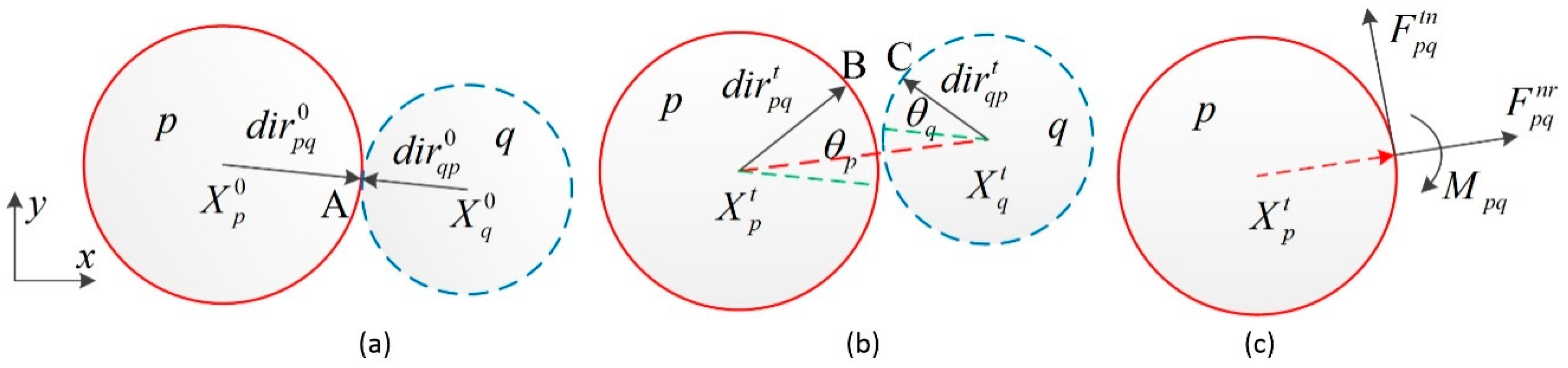
The contact particles are bonded together by the bonds, which can resist normal force, shear force and bending moment. As shown in Figure 1a, particle p and particle q are in contact with each other at point A at the original states. and are their coordinates respectively. and are the vectors pointing from their centers to the contact point A respectively. At time t, the two particles move to new positions and , as shown in Figure 1b. The contact point A on particle p move to point B and the point A on particle q move to point C. The vector and the vector rotate to and , respectively. In addition, and are rotation angles of particles p and q in time t respectively, defining anticlockwise as positive direction. The contact forces and moment applied to particle p from particle q via the bond are normal force , shear force and moment , as shown in Figure 1c.
The shear force and moment are determined by the following equations:
where and are shear stiffness and bending stiffness respectively, is the original distance between p and q, is shear strain of the bond between p and q which is the ratio of deformation in tangential direction to . A nonlinear elastic tensile stiffness model is proposed to describe the relationship between normal force and normal strain undergoing tension. Then the force in normal direction is expressed as:
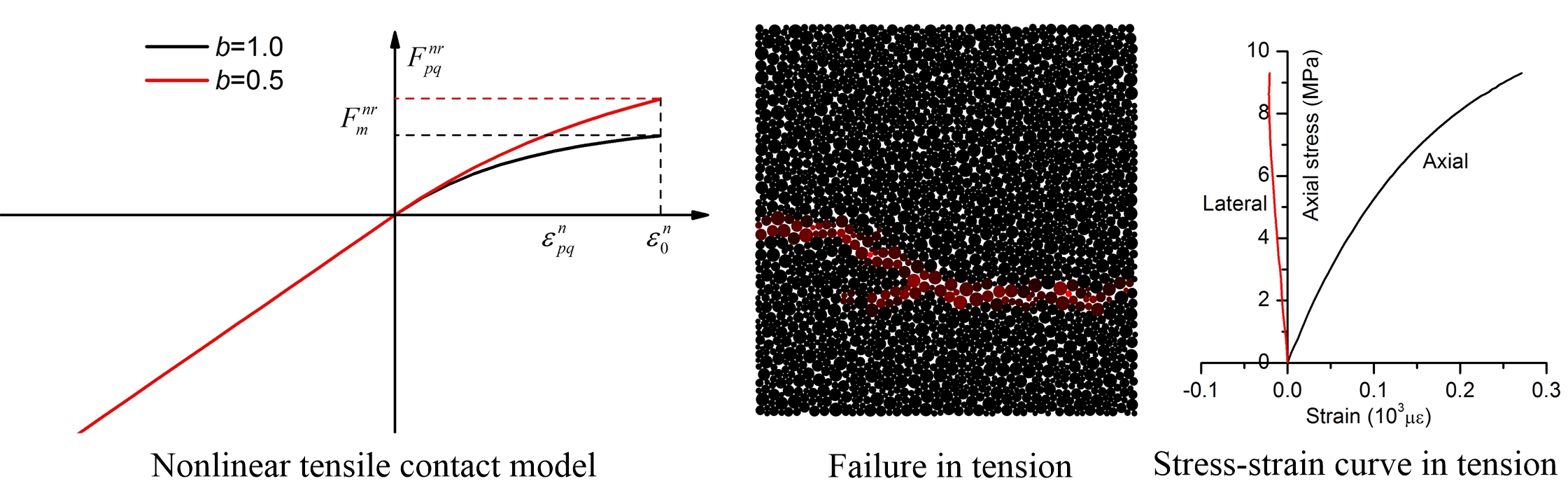
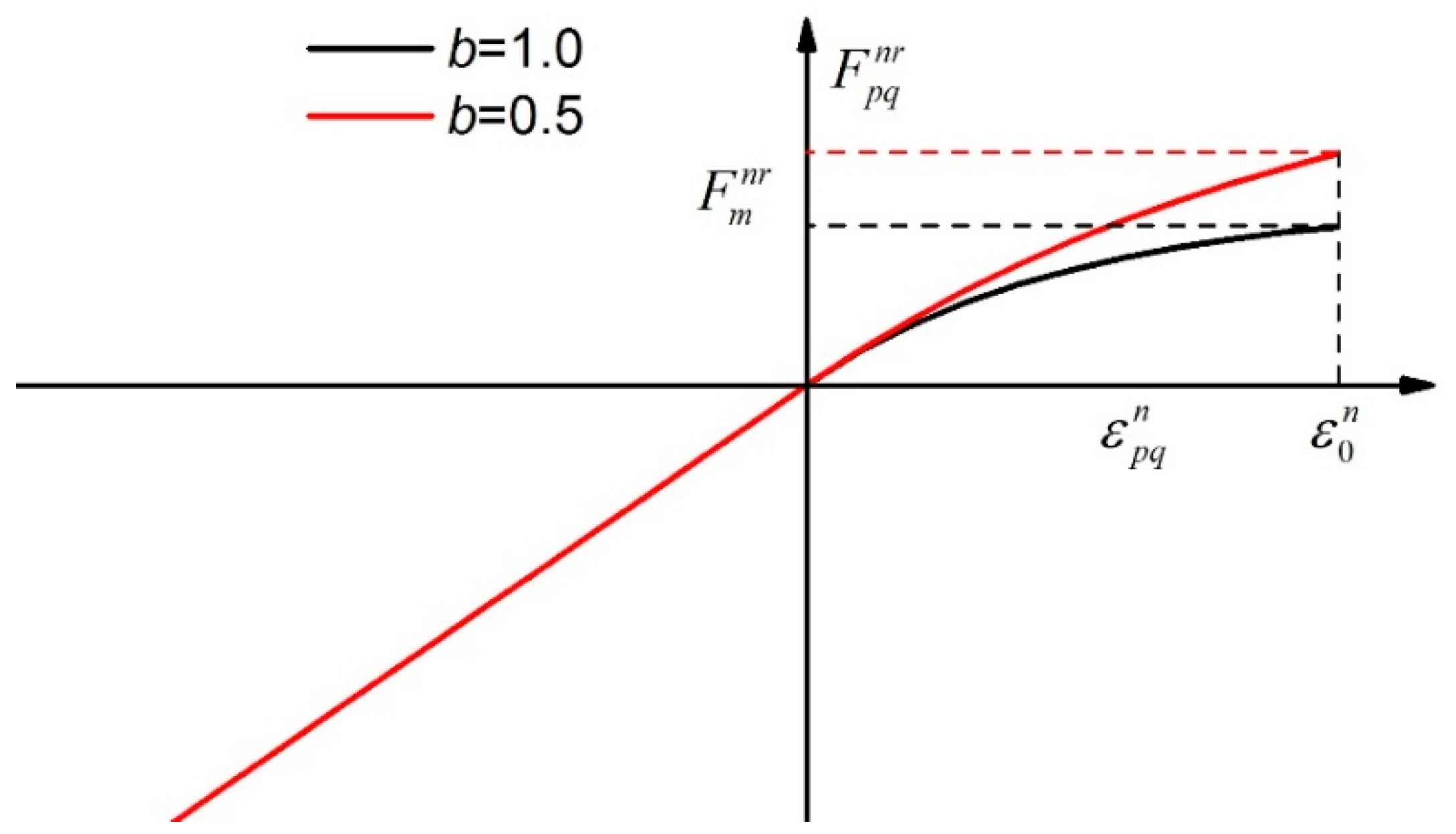
where is normal stiffness, is normal strain of the bond between p and q, the b is shape coefficient of the nonlinear elastic model and is the ultimate normal tensile strain. Figure 2 presents the relationship between normal force and normal strain with different value of b. The value of b has great effect on the normal force versus normal strain curve and the ultimate normal tensile force, . and which is the increment of in each time step are given by:
where is the distance between the centers of p and q at time t, and are the radii of particles p and q respectively, and are the centroid displacements of particles p and q respectively, is an unit vector obtained by rotating the unit vector which points to the center of q from the center of p 90 degrees in the anticlockwise direction, is time step.
Another modification to the BPM is that the bonds are assumed as many tiny elastic beams, which distribute between two contact particles in a region wide 2wrm and are parallel to the center line of the two particles, as presented in Figure 3, where the w is bond width coefficient, rm is the smaller one of rp and rq. The range of w is from 0 to 1 and that w equals 0 means all the tiny beams gather in the center line of the two contact particles. Bonds with different bending stiffness but with the same normal stiffness and shear stiffness can be modelled by changing the distribution of the tiny beams.
The modified Mohr-Coulomb criterion with a tension cut-off and an upper bound is used for the shear strength of the bonds, as shown in Figure 4, where is the upper bound of shear strain, is the ultimate pure shear strain of the bond, is the internal friction angle and is the friction angle between particles when the bond between them fails. In this paper, the stresses are replaced by the strains in order to obtain better simulation results by cooperating with the nonlinear tensile model and the effect of the bend on the tensile strain is taken into consideration as follows.
If the bond is broken or no bond exists between particles p and q which contact with each other, then only normal force and shear force exist between them. The normal force is calculated by Equations (3) and (4). in Equation (4) should be replaced by the sum of the radii of p and q. The shear force is calculated as follows:
where is the coulomb friction coefficient.
The resultant contact force vector and the resultant contact moment on particle p are calculated as follows:
where is an unit vector pointing from the center of particle p to the center of particle q. is a set of particles which are in contact with particle p.
2.2. Numerical Simulation Model
The disc-shaped particles are considered as rigid bodies and their translational motions and rotational motions are governed by the standard equations of rigid body dynamics:
where and are the external force vector and external moment applied to particle p respectively. and are mass and moment of inertia of particle p respectively. and are damping force and damping moment respectively, which are introduced to dissipate kinetic energy and gain a quasi-static state of equilibrium of the particles and are expressed as [34]:
where and are translational and rotational damping constant respectively. The centroid displacement and rotation angle of particle p can be obtained by using an explicit central difference method to integrate Equations (10) and (11). The algorithm is described as follows:
where the superscript indicates th step. should not exceed the critical time step to remain numerical stability as introduced in [34].
The forces and moments are transmitted through the contacts between particles or the contacts between particles and plates. There are two kinds of particle contacts according to whether an effective bond exists between the contact particles: the bonded particle contacts and the unbonded particle contacts. Two particles p and q are bonded together in the original rock specimens if their relative position satisfies the Equation (18):
where is a nonnegative constant defined by user to eliminate the numerical errors caused during the particle generating. The errors may result in separation of two particles which should touch each other. A bond is created between every bonded particles. If is too large, it would lead to forming bond between two particles far away from each other. In our model, = 0.001 is suggested. When the bond is broken, the bonded particle contact becomes unbonded particle contact. Furthermore, two particles p and q which are not close to each other may approach each other during the simulation process, and form an unbonded particle contact when their relative position satisfies the Equation (19):
The forces and moments on the bonded particle contacts are calculated by Equations (1)–(3). While forces on the unbonded particle contacts, where no moment exists are calculated by Equations (3) and (7). The bonded particle contacts are identified at the beginning of the simulation and updated in each time steps if any bond is broken. The unbonded contacts should be identified in every time steps.
In order to improve the computational efficiency, background grids and cells are introduced in searching particle contacts. In each step, all the particles are stored in the cells formed by the grids according to their centroid position coordinates. The cell size is equal to , where is the maximum radius of the particles and is a user-defined parameter, which is positive and very small to obtain high searching efficiency. The suggested value for is 0.01 in our model. A particle can only form a particle contact with particles located in the same cell with it and with particles located in the neighbor cells. To avoid duplicate calculation, particles in cell j are only used to try to form particle contacts with particles in cell j or in neighbor cells whose numbers are larger than j.
2.3. Dimensionless Parameters in NET-BPM
In the conventional BPM, the micro parameters are normal stiffness , shear stiffness , bending stiffness , ultimate normal strain , ultimate pure shear strain , upper bound of shear strain , ultimate relative rotation angle , friction angles and , translational damping constant and rotational damping constant , etc. The macro parameters are UCS, TS, the ratio of UCS/TS, Young’s modulus E and Poisson’s ratio v, etc. A few more micro parameters, which are w and b are included in the NET-BPM. In addition, because Young’s modulus and Poisson’s ratio in compression and tension are different, they are denoted as Ec and Et, vc and vt, respectively. In this paper, the effects of particle size, particle arrangement, porosity and density of the specimens are not investigated. Young’s modulus and Poisson’s ratio discussed here are the apparent ones. By using dimensionless analysis similar to [28,34], the dimensionless micro parameters are ks/kn, km/(knR), , , , , w, b, and the dimensionless macro parameters are EcR2/kn, vc, , , Et/Ec, vt/vc in our model. R is the characteristic length which is equal to Rmax. As the nonlinear elastic model is applied, the ratio of Ec to Et and the ratio of vc to vt are not equal to 1 anymore, so Et/Ec and vt/vc should be taken into consideration.
2.4. Specimen Preparation
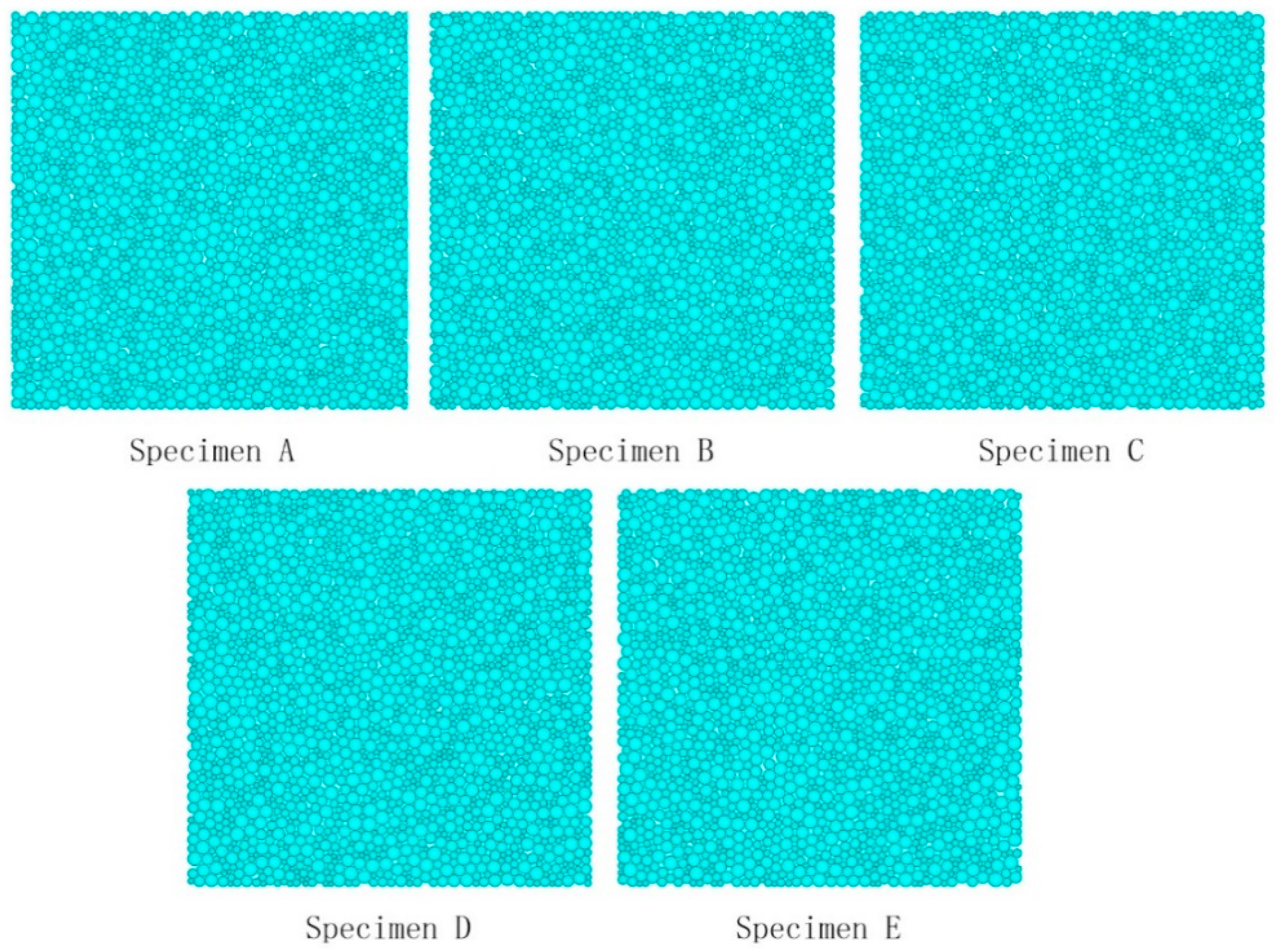
Uniaxial compression tests and direct tension tests are simulated in this study. The rock specimens used for simulations are created by the particle generating method proposed in [44], which can create dense and stable particle packings with disks once the geometric contour of the specimen and the minimum and maximum particle size are given. The effect of the size of particles and specimens on our method is not concerned in this study. Thus, square specimens with length L = 50 mm created by the method from [44] with Rmax = 0.9 mm and minimum particle radius Rmin = 0.3 mm are used for our simulations. Five specimens are created by using different seeds in the initiation of the particle generation, as shown in Figure 5. They are used to study the effects of the particle arrangement on the simulations. Some main parameters of the specimens are listed in Table 1, where Ra is the average radius of the particles and overlap ratio is the ratio of the overlap length to the sum of the radii of the two overlap particles.
As presented in Figure 6, when the uniaxial compression tests are simulated, the specimens are placed between two parallel plates which are considered as rigid bodies. The bottom one is fixed and the top one moves towards the bottom one with a given constant velocity, V. When the direct tension tests are simulated, the particles in the specimens near the top and bottom boundaries are fixed to the top and bottom plates respectively and have the same velocity with the plate. In order to eliminate the effect of the boundaries on the simulation results, a layer with a height of 0.6L in tensile direction and a width of L perpendicular to the tensile direction is defined, which located in the center of the specimens. Only the bonds existing between the particles located in this layer are allowed to fail, similar to that in [12]. The bottom plate is fixed and the top plate moves away from the bottom one with a constant velocity V. The lateral strain of the specimens is determined by the displacement of two particle groups. One particle group consists of four particles, which are closer to the middle point of the left side boundary of the specimen than other particles at the initial time. The other particle group consists of four particles, which are closer to the middle point of the right side boundary than other particles. The average distance of the two groups of particles in the direction perpendicular to the loading direction at the initial time and its variation during simulations are used to calculate the lateral strain. The axial strain is determined by the displacement of the two rigid plates. The loads are calculated by averaging the forces on the top and bottom plates. UCS and TS can be obtained by dividing the ultimate loads by the width of the specimen. The thickness of the specimen is assume to be 1 m in 2-D. Ec, Et, vc and vt are determined at the state when the load is equal to half the ultimate load and the secant lines are used to estimate them as introduced in [8,45,46].
The NET-BPM model is compiled in Fortran 90 language for simulating uniaxial compression tests and direct tension tests. The values of the micro parameters in the model are presented in Table 2. The density of the particles is set to be 2900 kg/m3. The critical time step = 2.5 × 10⁻⁸ s is obtained with the method introduced in [34] if the safety factor is set to 0.1. Thus, the time step = 10−8 s is proper in our model. The loading speed V = 0.1 m/s in both compression and tension tests. Damping constant and are set to be 0.02 which are proved to be large enough to guarantee the quasi-static state of equilibrium of the particles. All five specimens presented in Figure 5 are used for simulations with the micro parameters in Table 2.
A simulation case costs about two hours on a machine with an Intel Core 5 3.2 GHz Processor. The compressive loads and tensile loads of specimen A at different displacements are presented in Figure 7. The creak patterns of specimen A under compression and tension are shown in Figure 8. The tcm and ttm are the time when the loads reach their peak values in compression and tension, respectively. The color of the particle varies from black to red gradually according to the ratio of the present number to the original number of the bonded contacts on the particle, which varies from 1 to 0. Tensile failure is the dominant failure pattern of the bonded contacts in both uniaxial compression tests and direct tension tests. The number of the failed bonded contacts was 420 by the time t = tcm, which increased sharply to 931 after 10,000 time steps in compression test. The number of the failed bonded contacts was 7 by the time t = ttm, which increased sharply to 88 after 4000 time steps in tension test. Only one main crack appeared in tension test, which is almost perpendicular to the tensile direction, but several oblique cracks appeared in compression tests. All cracks observed in our simulation are similar to those observed in experiments presented in [47,48].
The properties of specimen A–E from the simulations are listed in Table 3. It shows that the difference of the properties between different specimens is small. The maximum ratio of the stand deviation value to the average value is 0.15. This indicates that the specimens created by the method in [44] with the same Rmax and Rmin share almost the same properties.
3. Relationship between Micro and Macro Parameter
In this Section, the relationships between micro and macro parameters in the NET-BPM introduced in Section 2.3 are investigated, which are revealed by simulating the uniaxial compression tests and direct tension tests with different values of one or two micro parameters. If not specified particularly, the values of the micro parameters are the same as those in Table 2. In order to eliminate the effects of the particle arrangement, specimen size and particle size on the simulations, specimen A introduced in Section 2.4 is used for all the simulations.
3.1. Effect of Bond Stiffness on Macro Parameters
Changing the value of ks/kn from 0.1 to 1.0 with km/(knR) equal to 0.064, 0.160 and 0.256, different values of the macro parameters can be observed. The relationships between the macro parameters and ks/kn at different km/(knR) are presented in Figure 9. The results show that Ec increases with the increasing of ks/kn at different values of km/(knR), and vc decreases with the increasing of ks/kn. The trends are in accord with those in [28,29,34]. With the values of the ks/kn changing from 0.1 to 1.0, Poisson’s ratio decreases from 0.45 to 0. The effects of the bending stiffness on Ec and vc are very small and can be ignored. However, increasing the bending stiffness can enhance the strength (UCS and TS) of the specimens and increase UCS/TS distinctly when ks/kn is higher than 0.4, as shown in Figure 9c–e. The values of ks/kn and km/(knR) have very small effects on the value of Ec/Et, as shown in Figure 9f, and small effects on the value of vc/vt.
3.2. Effect of Shape Coefficient on Macro Parameters
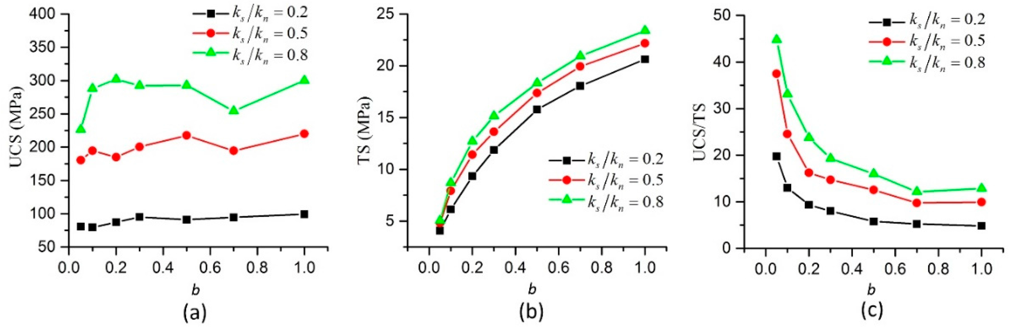
As presented in Figure 2b is a very important micro parameter whose effects on macro parameters are investigated by changing its value from 0.05 to 1.0 with ks/kn equal to 0.2, 0.5 and 0.8 in the simulations. The results are presented in Figure 10 and Figure 11.
The results show that with the increasing of b, TS increases but UCS almost remains unchanged and the value of UCS/TS decreases. The effects of b on TS and UCS/TS decrease with the increasing of b and when b is larger than 0.5, the effects become very small, as shown in Figure 10. By choosing a small b, e.g., b = 0.05, a value of UCS/TS as large as 45 can be obtained to meet the practical values of many hard rocks, which is difficult to achieve by the conventional BPM [14]. The value of b has distinct effects on the value of Et, while small effects on the value of Ec, as shown in Figure 11a,b. Decreasing b from 1.0 to 0.05 results in increasing of Ec/Et from 1.05 to 1.6 in our study at different values of ks/kn, as shown in Figure 11c. Similar to the Young’s modulus, the Poisson’s ratio are also affected by the value of b. Increasing of b leads to decrease of vc, increasing of vt and sharply decreasing of vc/vt, as shown in Figure 11d–f. The value of vc/vt can reach 4.5 when b is 0.05. When b is larger than 0.7, the variation of b has small effect on the macro parameters.
3.3. Effect of Bond Width Coefficient on Macro Parameters
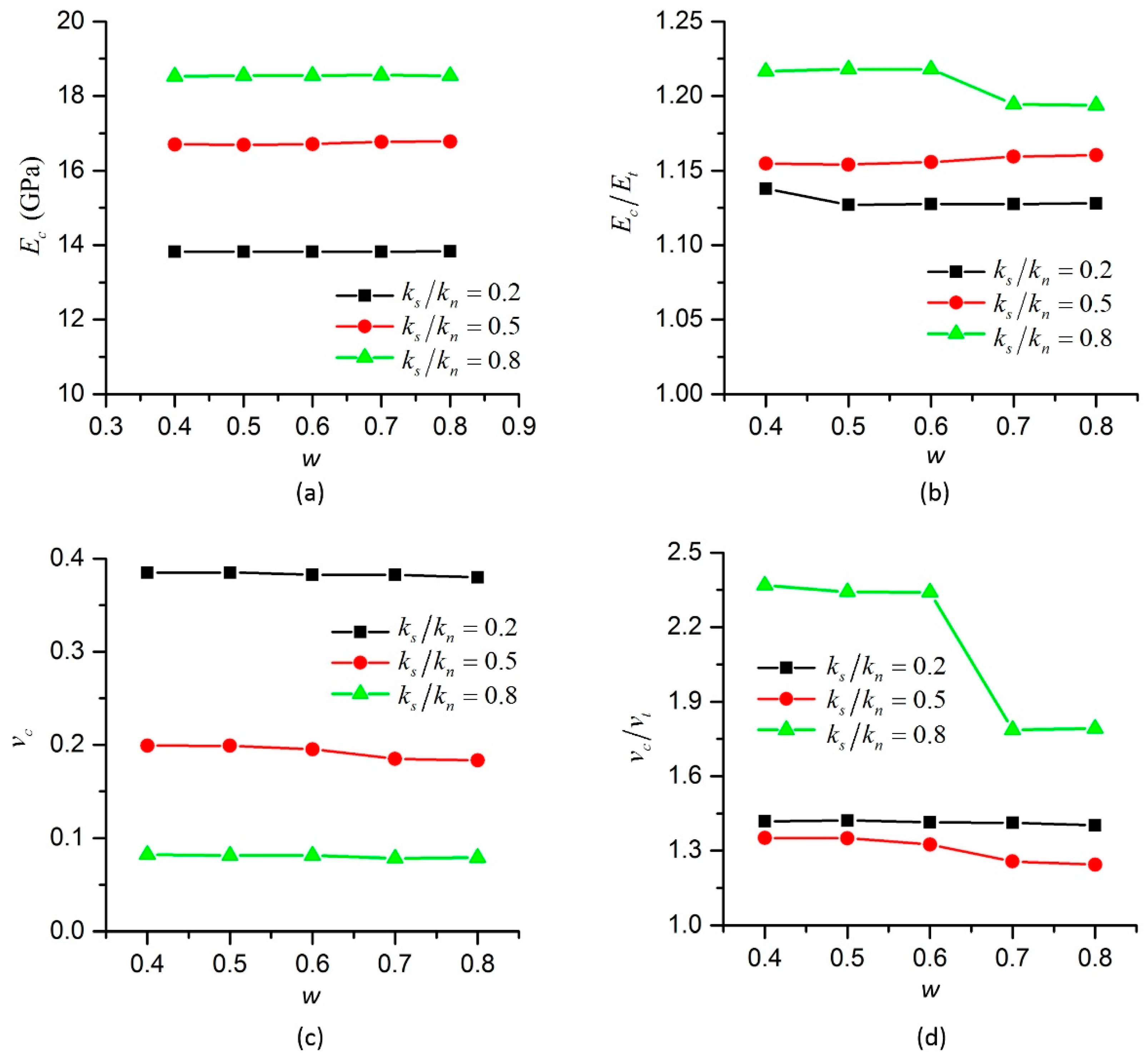
The effects of w on macro parameters are investigated by changing its value from 0.4 to 0.8 with ks/kn = 0.2, 0.5 and 0.8. In order to guarantee the identical value of km/(knR) in all the cases, the distributions of the tiny beams in the bonds are changed according to the value of w. The simulation results are presented in Figure 12. The results show that the width of the bond has little effects on Young’s modulus and Poisson’s ratio, and has almost no effects on Ec and vc, as shown in Figure 12a–d. While larger w leads to smaller UCS, as shown in Figure 12e, and has almost no effect on TS, thus results in smaller UCS/TS, as shown in Figure 12f. Noticing Equation (6), if the relative rotation angle is not zero, larger w indicates smaller when the bond fails, that means smaller tensile forces in the bonds. However, this relationship is not shown in the simulated tension tests because the relative rotation angles between contact particles are very small in the tension tests. While in the compression tests, the relative rotation angles are large enough to affect the strength of the specimens and the major failure type of the bonds is tensile failure.
3.4. Effect of Ultimate Pure Shear Strain on Macro Parameters
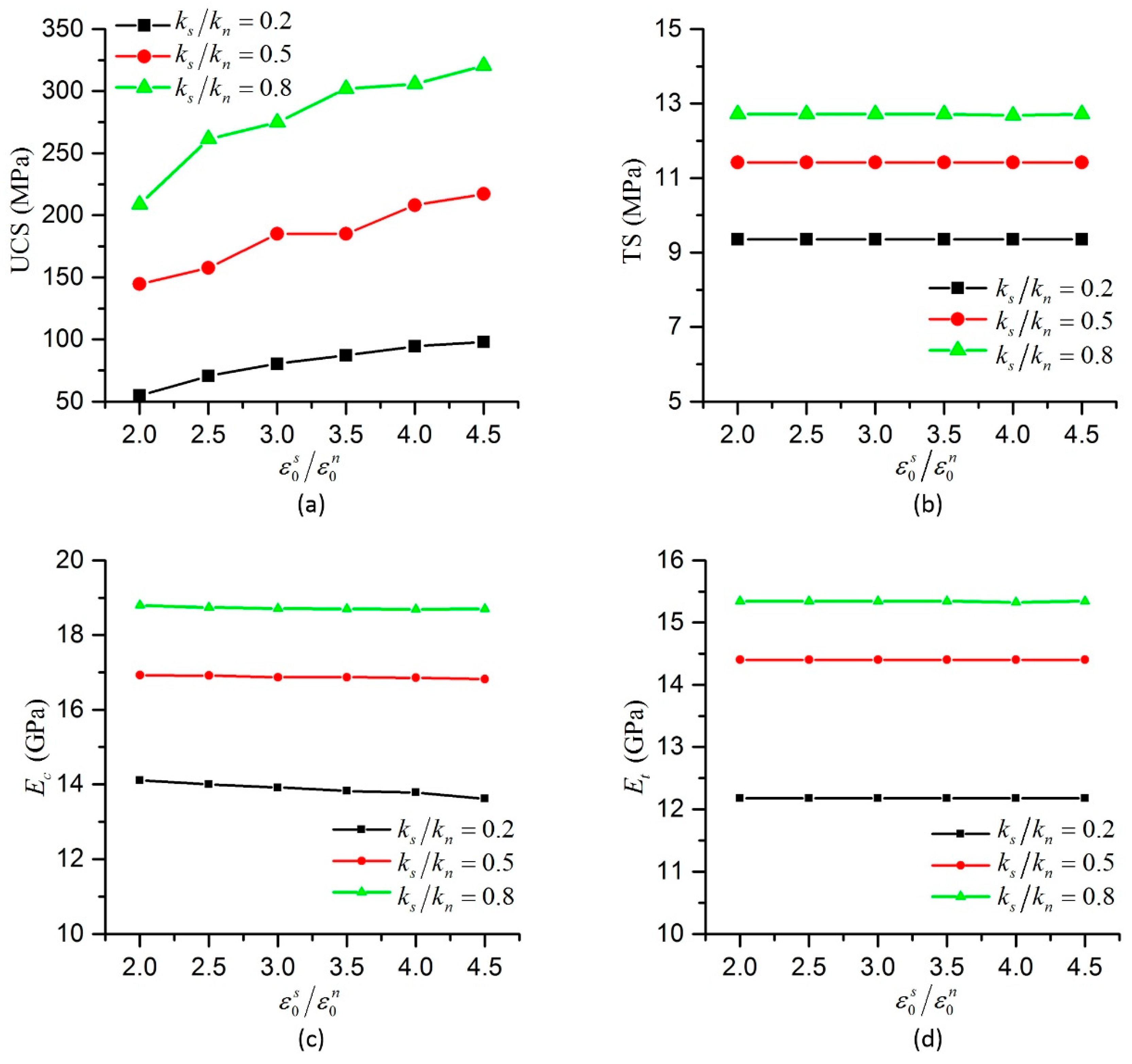
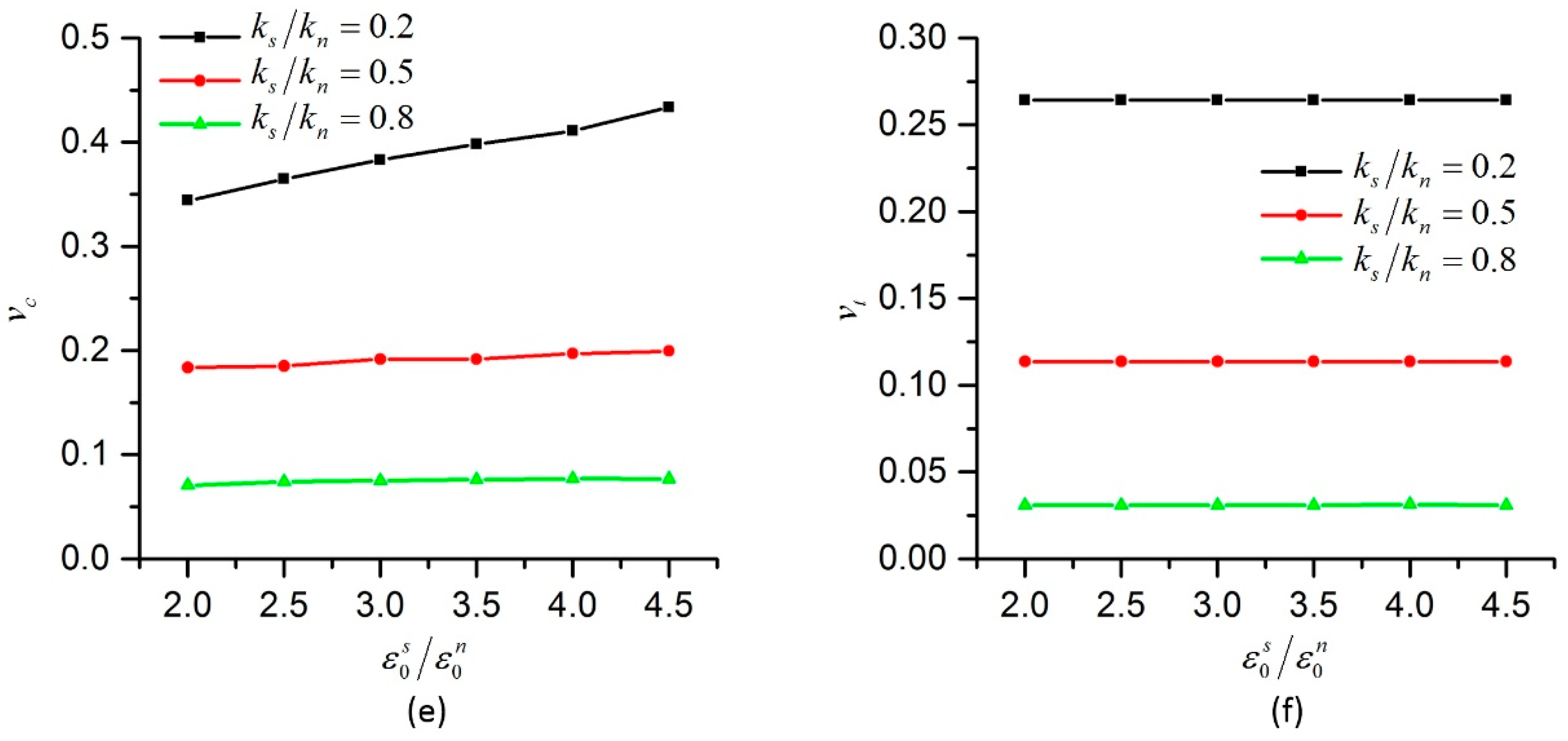
The ultimate pure shear strain has great effects on UCS, as shown in Figure 13a. Changing from 2.0 to 4.5 with ks/kn equal to 0.2, 0.5 and 0.8, UCS increases by more than 50%, but TS, Et and vt remain the same, as shown in Figure 13b,d,f. Increasing can decrease Ec and increase vc, but the effects are very small and can be ignored, as shown in Figure 13c,e.
4. Application of the NET-BPM
In this section, the Lac du Bonnet (LDB) granite which are widely used for model calibration and a quartzite studied in [39] under uniaxial compression and direct tension are modelled with the NET-BPM. Firstly, two specimens are created and the micro parameters in our model are determined for the two rocks. Then the simulation results of LDB granite and the quartzite are compared with the experimental results.
4.1. Modelling LDB Granite
A rock specimen with the size same as that in [42] is created using the method in [44] with Rmax = 0.9 mm and Rmin = 0.3 mm. The effect of particle size is not discussed in this study, so the particle size same as that in Section 3 is adopted. The parameters of the specimen for LDB granite are listed in Table 4. The properties of the LDB granite are presented in Table 5, where Young’s modulus are from [49], and the rest of the data are from [42]. It should be noticed that Young’s modulus and Poisson’s ratio are converted to the apparent values.
From the investigation in Section 3, we know that b is the major factor affecting the values of Ec/Et, and that b and ks/kn is the major factor affecting the values of vc. Combining Figure 9b and Figure 11c,d, the values of b and ks/kn can be roughly estimated to satisfy that vc = 0.35 and Ec/Et = 1.43. Then kn can be estimated by amplifying initial value in Section 3 to obtain that Ec = 68.1 GPa. The next step is to get an appropriate value of so that TS = 9.3 MPa is obtained. The last step is to guarantee that UCS = 200 MPa, which can be achieved by choosing proper values of km/(knR), w and . Proper micro parameters in NET-BPM for LDB granite can be obtained through several simulations and modifications, as shown in Table 6. The macro parameters obtained are presented in Table 5.
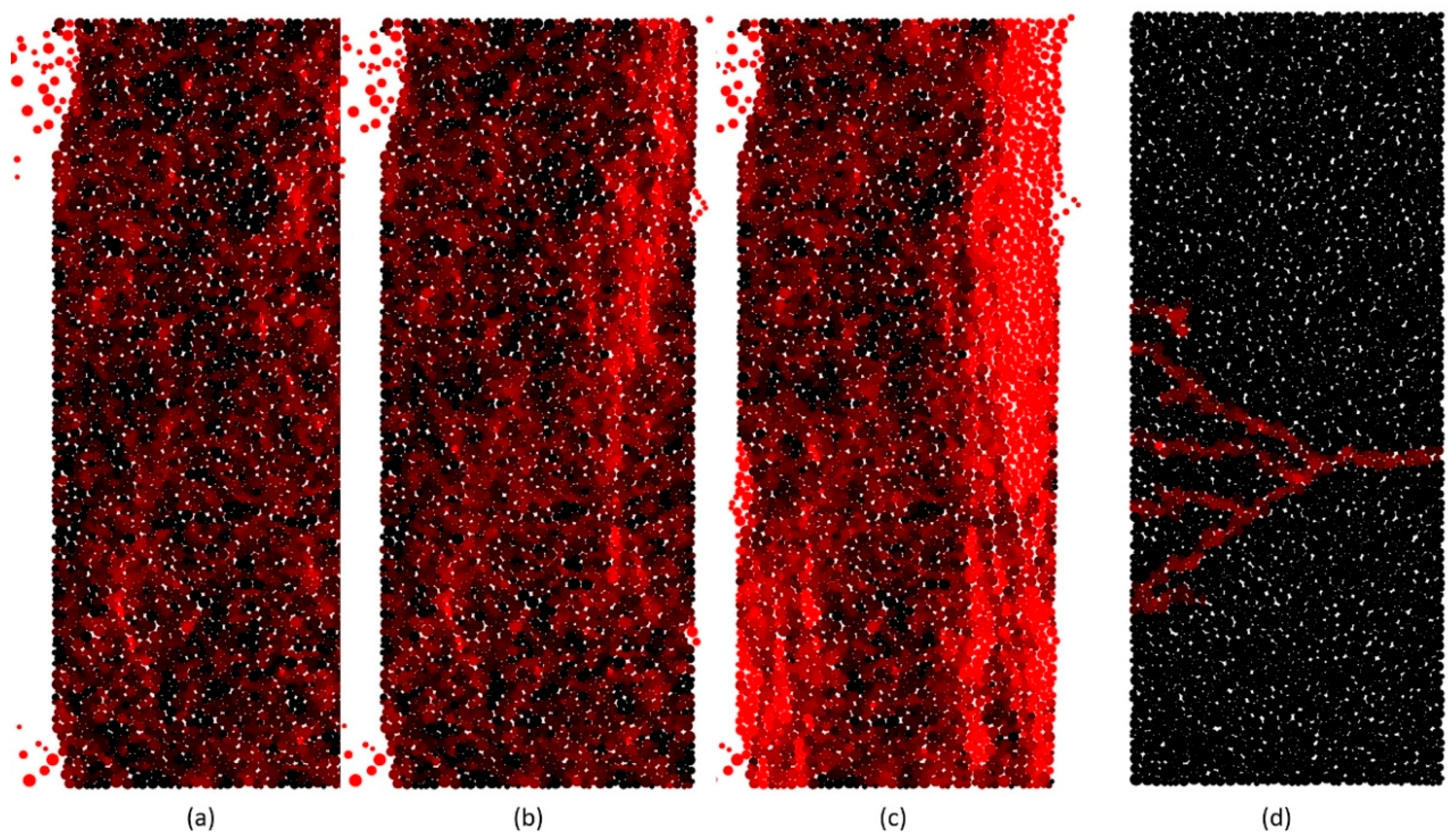
As the ultimate axial strain in tensile test is small, a lower loading speed of 0.01 m/s is applied in direct tensile tests. The results show that not only Ec, vc, UCS, TS and UCS/TS from the NET-BPM model are in good agreement with the experimental values, which is achieved in [14], but also Et and Ec/Et are in good agreement with the experimental values. The stress-strain curves of the LDB granite under uniaxial compression test from our method are similar to those from experiments in [42], as shown in Figure 14. The crack patterns of LDB granite under compression and tension tests are shown in Figure 15. Same method introduced in Section 2.4 is used to present the cracks. Figure 15a shows the cracks at the time when the compressive load reaches its peak. After that, the cracks develop quickly. Most of them are oblique. Figure 15d shows the cracks at time when the tensile load reaches its peak. The cracks extend perpendicular to the loading direction quickly, which results in the fracture of the specimen.
4.2. Modelling of Quartzite
A rock specimen with the size same as that in [39] is created using the method in [44]. Since the width of the specimen is only 31 mm, Rmax = 0.6 mm and Rmin = 0.2 mm are used for the specimen preparation. The parameters of specimen for the quartzite are listed in Table 4. The properties of the quartzite from experiments in [39] are listed in Table 5. Similar to that in Section 4.1, a set of micro parameters is obtained in order to get a response close to the quartzite, as listed in Table 6.
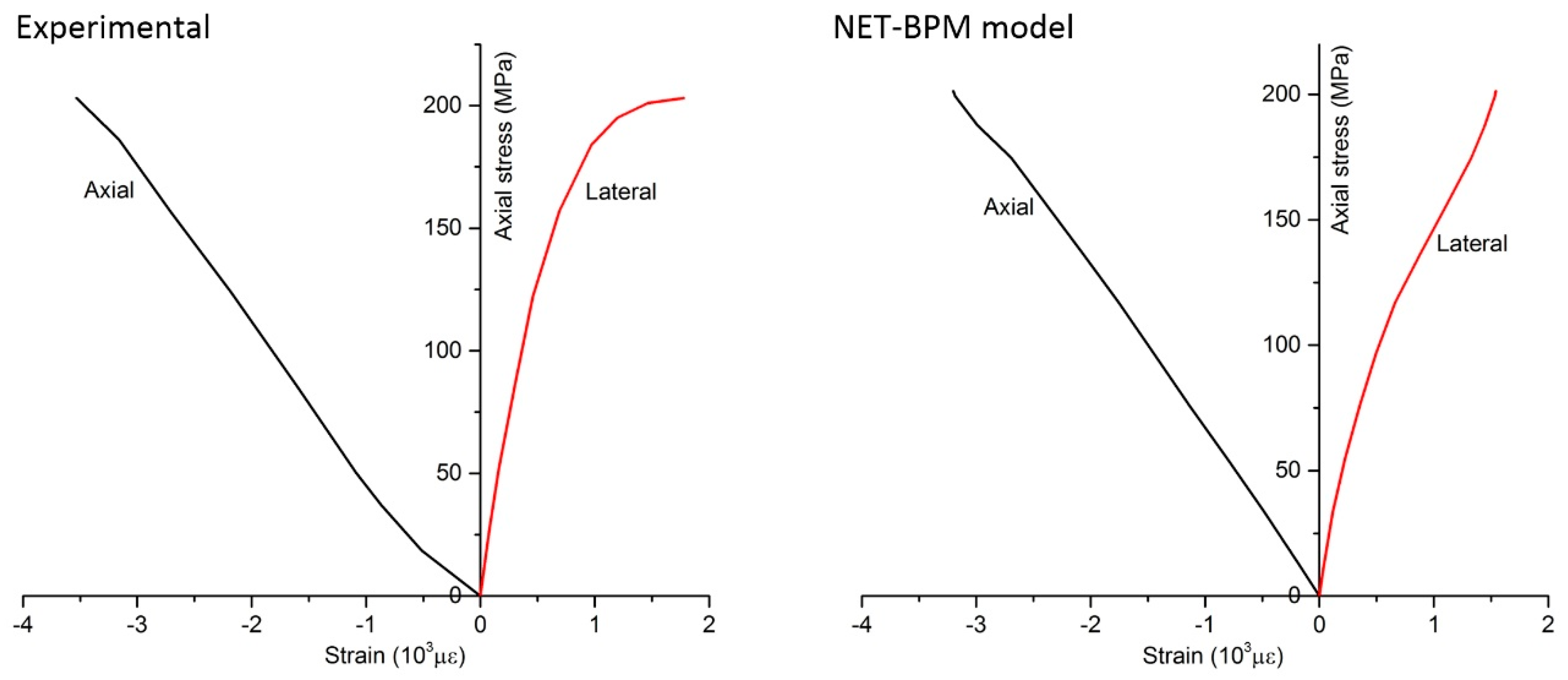
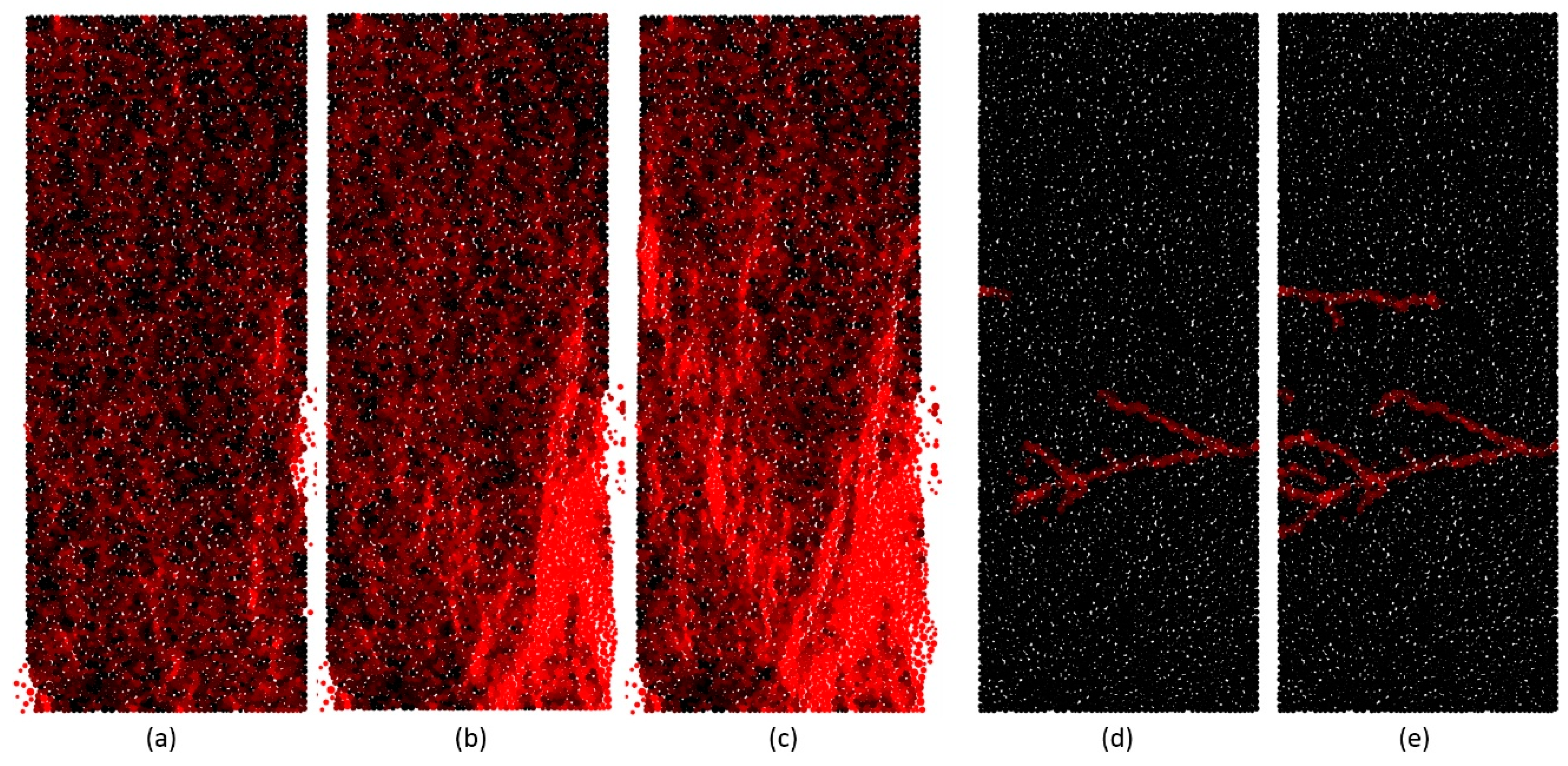
A loading speed V = 0.01 m/s is used in the direct tension tests. The properties of the specimen from our simulations are listed in Table 5. All the properties from simulations are in good agreement with those from experiments. The stress-strain curves of the quartzite under compression and tension are presented in Figure 16. The stress-strain curves of sample C-Q1 and sample T-Q1 in [39] are presented for comparison. The results show that the stress-strain curves of the specimen modelled by the NET-BPM are in good agreement with those of the quartzite. The stress-strain curve of the quartzite under direct tension tests is nonlinear, which is reproduced well by our model. The crack patterns of the quartzite in the simulations are presented in Figure 17. Most of the cracks under compression are parallel to the loading direction, which is different from that in the simulation of LDB granite. Even though failure pattern of sample C-Q1 is shear failure found in [39], split failure pattern is observed in another sample, C-Q2 under uniaxial compression loading. The cracks of the quartzite form a line perpendicular to the loading direction, which results in failure of the specimen. This is in accord to experimental results in [39].
5. Conclusions
In this paper, a new model is proposed for rock-like materials, which is named as NET-BPM model. The NET-BPM model, which adopts nonlinear tensile stiffness and a new form of bonds in its contact model, has the following advantages. (1) It is very difficult to gain a large ratio of UCS/TS more than 20 in conventional BPM model [1,2,20]. However, compared to our model, a large range of UCS/TS ratio (from 5 to 45 in the presented simulations) can be obtained by using different b and ; (2) The nonlinear behavior of some rocks under direct tension, which is observed in many experiments [8,36,37,38,39,40], can be reproduced well in our model with a proper b; (3) The differences between Young’s modulus, Poisson’s ratio of specimens, when they are under compression and tension, which are observed in experiments [38,41,49,50], are captured well in the NET-BPM model. e.g., the value of Ec/Et ranging from 1.0 to 1.6 can be obtained; (4) It is possible to change the width of the bond without changing the stiffness of the bond in the NET-BPM model, which helps to obtain different UCS without affecting TS and Ec.
The relationships between micro and macro parameters in our model were investigated through simulating uniaxial compression tests and direct tension tests. And the tests were performed upon specimens sharing identical particle arrangement. The results show that there is no significant difference for the effect of ks/kn on rock’s strength, Young’s modulus and Poisson’s ratio between our model and typical DEM model [28]. Larger ks/kn will results in larger Ec, UCS, TS and UCS/TS, and smaller vc. Besides ks/kn, km/(knR) also has great effects on UCS, TS and UCS/TS, and the effects will become larger with the increasing of ks/kn. It should be noted that the larger km/(knR) will results in greater UCS, TS and UCS/TS, while it still has ignorable effects on Young’s modulus and Poisson’s ratio. In present investigation, the parameter b has great effects on strength, Young’s modulus and Poisson’s ratio of specimens in tensile tests but small effects in uniaxial compressive tests. In conclusion to this, parameter b has great influences on TS, UCS/TS, Ec/Et and vc/vt. However, as the increasing of b, those effects will become smaller. In addition, the effect of the bond width coefficient w on UCS is obvious in the NET-BPM. When w increases, UCS will decrease, but TS, Ec and vc will remain unchanged. Moreover, the ultimate shear strain has great effects on UCS, but very small effect on TS, Ec, Et, vc and vt. Increasing ultimate shear strain will increase UCS and results in larger UCS/TS.
The LDB granite and a quartzite under uniaxial compression tests and direct tension tests were modelled by the NET-BPM model. All the properties, including Ec, Et, vc, UCS, TS and UCS/TS from simulations are in good agreement with those from experiments. In addition, the stress-strain curves of LDB granite and the quartzite are also reproduced correctly. All those results indicate that NET-BPM is a very suitable method for modelling the deformation and fracture of rock-like materials.
Some work in the subsequent studies are listed as follows. (1) The effects of particle size and particle size ratio on the simulation results, which are not concerned in this work, need to be investigated. (2) More simulations like biaxial and Brazilian tests need to be performed to validate our model. (3) The 3-D NET-BPM model needs to be established to broaden the application scope of the NET-BPM model.
Acknowledgments
This work was supported by the National Natural Science Foundation of China (Grant No. 51179104). Thanks Zheng Cheng for language help.
Author Contributions
Yiping Ouyang developed the original concept, proposed the new model and wrote the paper. Yiping Ouyang and Xinquan Chen programmed the simulation code and performed the numerical experiments. Qi Yang and Yiping Ouyang analyzed and discussed the simulation results.
Conflicts of Interest
The authors declare no conflict of interest.
References
- Potyondy, D.O.; Cundall, P.A. A bonded-particle model for rock. Int. J. Rock Mech. Min. Sci. 2004, 41, 1329–1364. [Google Scholar] [CrossRef]
- Cho, N.; Martin, C.D.; Sego, D.C. A clumped particle model for rock. Int. J. Rock Mech. Min. Sci. 2007, 44, 997–1010. [Google Scholar] [CrossRef]
- Potyondy, D.O. Simulating stress corrosion with a bonded-particle model for rock. Int. J. Rock Mech. Min. Sci. 2007, 44, 677–691. [Google Scholar] [CrossRef]
- Yoon, J. Application of experimental design and optimization to PFC model calibration in uniaxial compression simulation. Int. J. Rock Mech. Min. Sci. 2007, 44, 871–889. [Google Scholar] [CrossRef]
- Park, J.-W.; Song, J.-J. Numerical simulation of a direct shear test on a rock joint using a bonded-particle model. Int. J. Rock Mech. Min. Sci. 2009, 46, 1315–1328. [Google Scholar] [CrossRef]
- Schöpfer, M.P.J.; Abe, S.; Childs, C.; Walsh, J.J. The impact of porosity and crack density on the elasticity, strength and friction of cohesive granular materials: Insights from DEM modelling. Int. J. Rock Mech. Min. Sci. 2009, 46, 250–261. [Google Scholar] [CrossRef]
- Wang, Y.; Tonon, F. Modeling Lac du Bonnet granite using a discrete element model. Int. J. Rock Mech. Min. Sci. 2009, 46, 1124–1135. [Google Scholar] [CrossRef]
- Zhao, B.; Liu, D.; Xue, K. Experimental study on direct tension properties of red sandstone in Chongqing. Geotech. Investig. Surv. 2011, 2011, 9–12. [Google Scholar]
- Fakhimi, A.; Alavi Gharahbagh, E. Discrete element analysis of the effect of pore size and pore distribution on the mechanical behavior of rock. Int. J. Rock Mech. Min. Sci. 2011, 48, 77–85. [Google Scholar] [CrossRef]
- Su, O.; Ali Akcin, N. Numerical simulation of rock cutting using the discrete element method. Int. J. Rock Mech. Min. Sci. 2011, 48, 434–442. [Google Scholar] [CrossRef]
- Asadi, M.S.; Rasouli, V.; Barla, G. A bonded particle model simulation of shear strength and asperity degradation for rough rock fractures. Rock Mech. Rock Eng. 2012, 45, 649–675. [Google Scholar] [CrossRef]
- Scholtes, L.; Donze, F.-V. A DEM model for soft and hard rocks: Role of grain interlocking on strength. J. Mech. Phys. Solids 2013, 61, 352–369. [Google Scholar] [CrossRef]
- Brown, N.J.; Chen, J.-F.; Ooi, J. A bond model for DEM simulation of cementitious materials and deformable structures. Granul. Matter 2014, 16, 299–311. [Google Scholar] [CrossRef]
- Ding, X.; Zhang, L. A new contact model to improve the simulated ratio of unconfined compressive strength to tensile strength in bonded particle models. Int. J. Rock Mech. Min. Sci. 2014, 69, 111–119. [Google Scholar] [CrossRef]
- Park, B.; Min, K.-B. Bonded-particle discrete element modeling of mechanical behavior of transversely isotropic rock. Int. J. Rock Mech. Min. Sci. 2015, 76, 243–255. [Google Scholar] [CrossRef]
- Jiang, M.; Chen, H.; Crosta, G.B. Numerical modeling of rock mechanical behavior and fracture propagation by a new bond contact model. Int. J. Rock Mech. Min. Sci. 2015, 78, 175–189. [Google Scholar] [CrossRef]
- Scholtes, L.; Donze, F.-V. Modelling progressive failure in fractured rock masses using a 3D discrete element method. Int. J. Rock Mech. Min. Sci. 2012, 52, 18–30. [Google Scholar] [CrossRef]
- Zhu, H.P.; Zhou, Z.Y.; Yang, R.Y.; Yu, A.B. Discrete particle simulation of particulate systems: A review of major applications and findings. Chem. Eng. Sci. 2008, 63, 5728–5770. [Google Scholar] [CrossRef]
- Utili, S.; Nova, R. Dem analysis of bonded granular geomaterials. Int. J. Numer. Anal. Methods Geomech. 2008, 32, 1997–2031. [Google Scholar] [CrossRef]
- Fakhimi, A. Application of slightly overlapped circular particles assembly in numerical simulation of rocks with high friction angles. Eng. Geol. 2004, 74, 129–138. [Google Scholar] [CrossRef]
- Ergenzinger, C.; Seifried, R.; Eberhard, P. A discrete element model to describe failure of strong rock in uniaxial compression. Granul. Matter 2011, 13, 341–364. [Google Scholar] [CrossRef]
- Jiang, M.J.; Yu, H.-S.; Harris, D. A novel discrete model for granular material incorporating rolling resistance. Comput. Geotech. 2005, 32, 340–357. [Google Scholar] [CrossRef]
- Jiang, M.J.; Yu, H.S.; Harris, D. Bond rolling resistance and its effect on yielding of bonded granulates by DEM analyses. Int. J. Numer. Anal. Methods Geomech. 2006, 30, 723–761. [Google Scholar] [CrossRef]
- Jiang, M.; Shen, Z.; Wang, J. A novel three-dimensional contact model for granulates incorporating rolling and twisting resistances. Comput. Geotech. 2015, 65, 147–163. [Google Scholar] [CrossRef]
- Tran, V.T.; Marin, P. A discrete element model of concrete under high triaxial loading. Cement Concr. Compos. 2011, 33, 936–948. [Google Scholar] [CrossRef]
- Tavarez, F.A.; Plesha, M.E. Discrete element method for modelling solid and particulate materials. Int. J. Numer. Methods Eng. 2007, 70, 379–404. [Google Scholar] [CrossRef]
- Matsuda, Y.; Iwase, Y. Numerical simulation of rock fracture using three-dimensional extended discrete element method. Earth Planets Space 2002, 54, 367–378. [Google Scholar] [CrossRef]
- Fakhimi, A.; Villegas, T. Application of dimensional analysis in calibration of a discrete element model for rock deformation and fracture. Rock Mech. Rock Eng. 2007, 40, 193. [Google Scholar] [CrossRef]
- Yang, B.; Jiao, Y.; Lei, S. A study on the effects of microparameters on macroproperties for specimens created by bonded particles. Eng. Comput. 2006, 23, 607–631. [Google Scholar] [CrossRef]
- Morgan, J.K. Numerical simulations of granular shear zones using the distinct element method—2. Effects of particle size distribution and interparticle friction on mechanical behavior. J. Geophys. Res. 1999, 104, 2721–2732. [Google Scholar] [CrossRef]
- Zhang, Q.; Zhu, H.; Zhang, L.; Ding, X. Study of scale effect on intact rock strength using particle flow modeling. Int. J. Rock Mech. Min. Sci. 2011, 48, 1320–1328. [Google Scholar] [CrossRef]
- Dondi, G.; Simone, A.; Vignali, V.; Manganelli, G. Numerical and experimental study of granular mixes for asphalts. Powder Tech. 2012, 232, 31–40. [Google Scholar] [CrossRef]
- Rojek, J.; Labra, C.; Su, O.; Oñate, E. Comparative study of different discrete element models and evaluation of equivalent micromechanical parameters. Int. J. Solids Struct. 2012, 49, 1497–1517. [Google Scholar] [CrossRef]
- Rojek, J.; Oñate, E.; Labra, C.; Kargl, H. Discrete element simulation of rock cutting. Int. J. Rock Mech. Min. Sci. 2011, 48, 996–1010. [Google Scholar] [CrossRef]
- Tropin, N.M.; Manakov, A.V.; Bocharov, O.B. Implementation of boundary conditions in discrete element modeling of rock cutting under pressure. Appl. Mech. Mater. 2014, 598, 114–118. [Google Scholar] [CrossRef]
- Lin, W.; Kamei, A.; Takahashi, M.; Kwasniewski, M.; Takagi, T.; Endo, H. Deformability of various granitic rocks from japan in uniaxial tension. In ISRM 2003—Technology Roadmap for Rock Mechanics; International Society for Rock Mechanics: Sandton, South Africa, 2003; pp. 787–790. [Google Scholar]
- Yu, X.-B.; Xie, Q.; Li, X.-Y.; Na, Y.-K.; Song, Z.-P. Cycle loading tests of rock samples under direct tension and compression and bi-modular constitutive model. Chin. J. Geotech. Eng. 2005, 27, 988–993. [Google Scholar]
- Yu, X.-B.; Wang, Q.-R.; Li, X.-Y.; Xie, Q.; Na, Y.-K.; Song, Z.-P. Experimental research on deformation of rocks in direct tension and compression. Rock Soil Mech. 2008, 29, 18–22. [Google Scholar]
- Li, D.; Li, X.; Li, C.C. Experimental studies of mechanical properties of two rocks under direct compression and tenslon. Chin. J. Rock Mech. Eng. 2010, 29, 624–632. [Google Scholar]
- Fujii, Y.; Takemura, T.; Takahashi, M.; Lin, W. Surface features of uniaxial tensile fractures and their relation to rock anisotropy in inada granite. Int. J. Rock Mech. Min. Sci. 2007, 44, 98–107. [Google Scholar] [CrossRef]
- Perkins, T.K.; Krech, W.W. The energy balance concept of hydraulic fracturing. Soc. Pet. Eng. 1968, 8, 1–12. [Google Scholar] [CrossRef]
- Martin, C.D. The Strength of Massive Lac du Bonnet Granite around Underground Openings; University of Manitoba: Winnipeg, MB, Canada, 1993. [Google Scholar]
- Koyama, T.; Jing, L. Effects of model scale and particle size on micro-mechanical properties and failure processes of rocks—A particle mechanics approach. Eng. Anal. Bound. Elem. 2007, 31, 458–472. [Google Scholar] [CrossRef]
- OuYang, Y.P.; Yang, Q.; Yu, L. An efficient dense and stable particular elements generation method based on geometry. Int. J. Numer. Methods Eng. 2017, 110, 1003–1020. [Google Scholar] [CrossRef]
- Fairhurst, C.E.; Hudson, J.A. Draft isrm suggested method for the complete stress-strain curve for intact rock in uniaxial compression. Int. J. Rock Mech. Min. Sci. 1999, 36, 279–289. [Google Scholar]
- Lin, W.; Manabu, T. Anisotropy of strength and deformation of inada granite under uniaxial tension. Chin. J. Rock Mech. Eng. 2008, 27, 2463–2472. [Google Scholar]
- Basu, A.; Mishra, D.A.; Roychowdhury, K. Rock failure modes under uniaxial compression, Brazilian, and point load tests. Bull. Eng. Geol. Environ. 2013, 72, 457–475. [Google Scholar] [CrossRef]
- Li, H.; Li, J.; Liu, B.; Li, J.; Li, S.; Xia, X. Direct tension test for rock material under different strain rates at quasi-static loads. Rock Mech. Rock Eng. 2013, 46, 1247–1254. [Google Scholar] [CrossRef]
- Stimpson, B.; Chen, R. Measurement of rock elastic moduli in tension and in compression and its practical significance. Can. Geotech. J. 1993, 30, 338–347. [Google Scholar] [CrossRef]
- Haimson, B.C.; Tharp, T.M. Stresses around boreholes in bilinear elastic rock. Soc. Pet. Eng. 1974, 14, 145–151. [Google Scholar] [CrossRef]
Figure 1.
Bond between particles and its forces and moment: (a) original positons of p and q; (b) positions of p and q at time t; (c) contact forces and moment on p.
Figure 1.
Bond between particles and its forces and moment: (a) original positons of p and q; (b) positions of p and q at time t; (c) contact forces and moment on p.

Figure 2.
Normal force versus normal strain.

Figure 3.
Bonds between contact particles.
Figure 4.
Shear strength criterion for the NET-BPM (nonlinear elastic tensile bonded particle model).
Figure 4.
Shear strength criterion for the NET-BPM (nonlinear elastic tensile bonded particle model).

Figure 5.
Specimens with different particle arrangement.

Figure 6.
Models for uniaxial compression tests and direct tension tests.
Figure 7.
Load-displacement curves: (a) compression; (b) tension.
Figure 8.
Crack patterns in compressive and tensile tests.

Figure 9.
Effect of ks/kn on macro parameters at different km/(knR): (a) Effect of ks/kn on Ec; (b) Effect of ks/kn on vc; (c) Effect of ks/kn on UCS; (d) Effect of ks/kn on TS; (e) Effect of ks/kn on UCS/TS; (f) Effect of ks/kn on Ec/Et.
Figure 9.
Effect of ks/kn on macro parameters at different km/(knR): (a) Effect of ks/kn on Ec; (b) Effect of ks/kn on vc; (c) Effect of ks/kn on UCS; (d) Effect of ks/kn on TS; (e) Effect of ks/kn on UCS/TS; (f) Effect of ks/kn on Ec/Et.
Figure 10.
Effect of b on UCS (uniaxial compressive strength), TS (tensile strength) and UCS/TS at different ks/kn: (a) Effect of b on UCS; (b) Effect of b on TS; (c) Effect of b on UCS/TS.
Figure 10.
Effect of b on UCS (uniaxial compressive strength), TS (tensile strength) and UCS/TS at different ks/kn: (a) Effect of b on UCS; (b) Effect of b on TS; (c) Effect of b on UCS/TS.

Figure 11.
Effect of b on Young’s modulus and Poisson’s ratio at different ks/kn: (a) Effect of b on Ec; (b) Effect of b on Et; (c) Effect of b on Ec/Et; (d) Effect of b on vc; (e) Effect of b on vt; (f) Effect of b on vc/vt.
Figure 11.
Effect of b on Young’s modulus and Poisson’s ratio at different ks/kn: (a) Effect of b on Ec; (b) Effect of b on Et; (c) Effect of b on Ec/Et; (d) Effect of b on vc; (e) Effect of b on vt; (f) Effect of b on vc/vt.
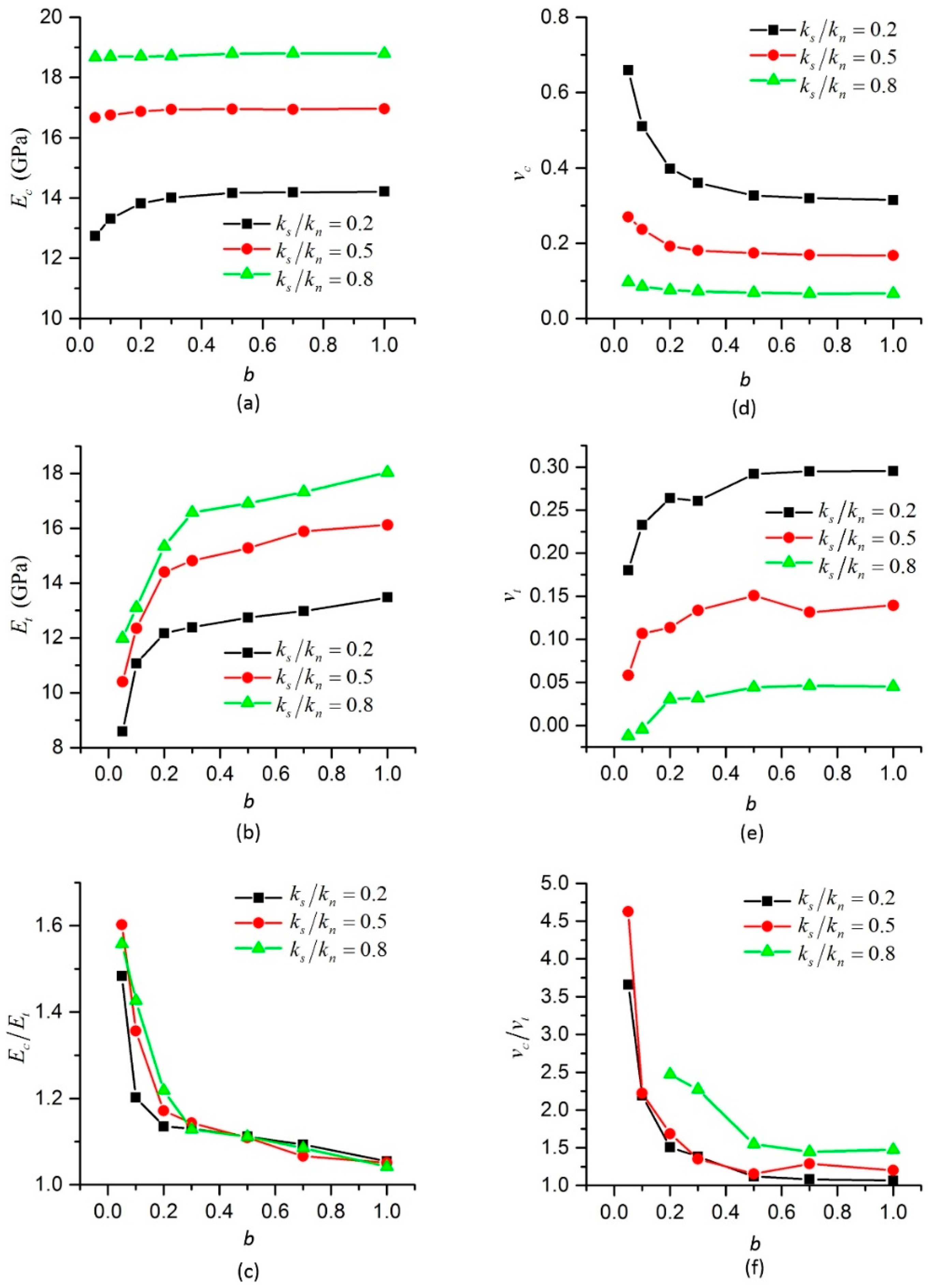
Figure 12.
Effect of w on macro parameters at different ks/kn: (a) Effect of w on Ec; (b) Effect of w on Ec/Et; (c) Effect of w on vc; (d) Effect of w on vc/vt; (e) Effect of w on UCS; (f) Effect of w on UCS/TS.
Figure 12.
Effect of w on macro parameters at different ks/kn: (a) Effect of w on Ec; (b) Effect of w on Ec/Et; (c) Effect of w on vc; (d) Effect of w on vc/vt; (e) Effect of w on UCS; (f) Effect of w on UCS/TS.

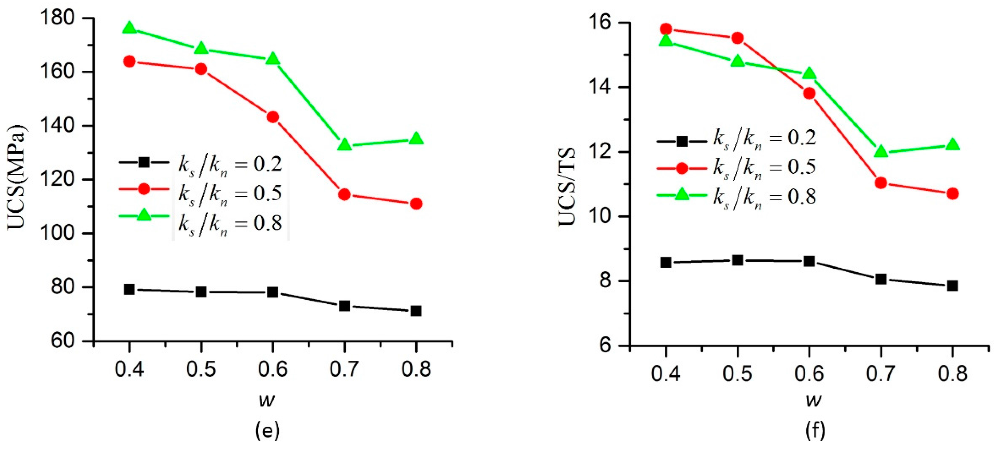
Figure 13.
Effect of ultimate pure shear strain on macro parameters at different ks/kn: (a) Effect of on UCS; (b) Effect of on TS; (c) Effect of on Ec; (d) Effect of on Et; (e) Effect of on vc; (f) Effect of on vt;.
Figure 13.
Effect of ultimate pure shear strain on macro parameters at different ks/kn: (a) Effect of on UCS; (b) Effect of on TS; (c) Effect of on Ec; (d) Effect of on Et; (e) Effect of on vc; (f) Effect of on vt;.


Figure 14.
Stress-strain curves of LDB (Lac du Bonnet) under compression from experiment and simulation.
Figure 14.
Stress-strain curves of LDB (Lac du Bonnet) under compression from experiment and simulation.

Figure 15.
Crack patterns of LDB under compression and tension: (a) Compression at t = tcm; (b) Compression at t = tcm + 10,000∆t; (c) Compression at t = tcm + 20,000∆t; (d) Tension at t = ttm; (e) Tension at t = ttm + 4000∆t.
Figure 15.
Crack patterns of LDB under compression and tension: (a) Compression at t = tcm; (b) Compression at t = tcm + 10,000∆t; (c) Compression at t = tcm + 20,000∆t; (d) Tension at t = ttm; (e) Tension at t = ttm + 4000∆t.

Figure 16.
Stress-strain curves of the Quartzite from experiment and simulation.
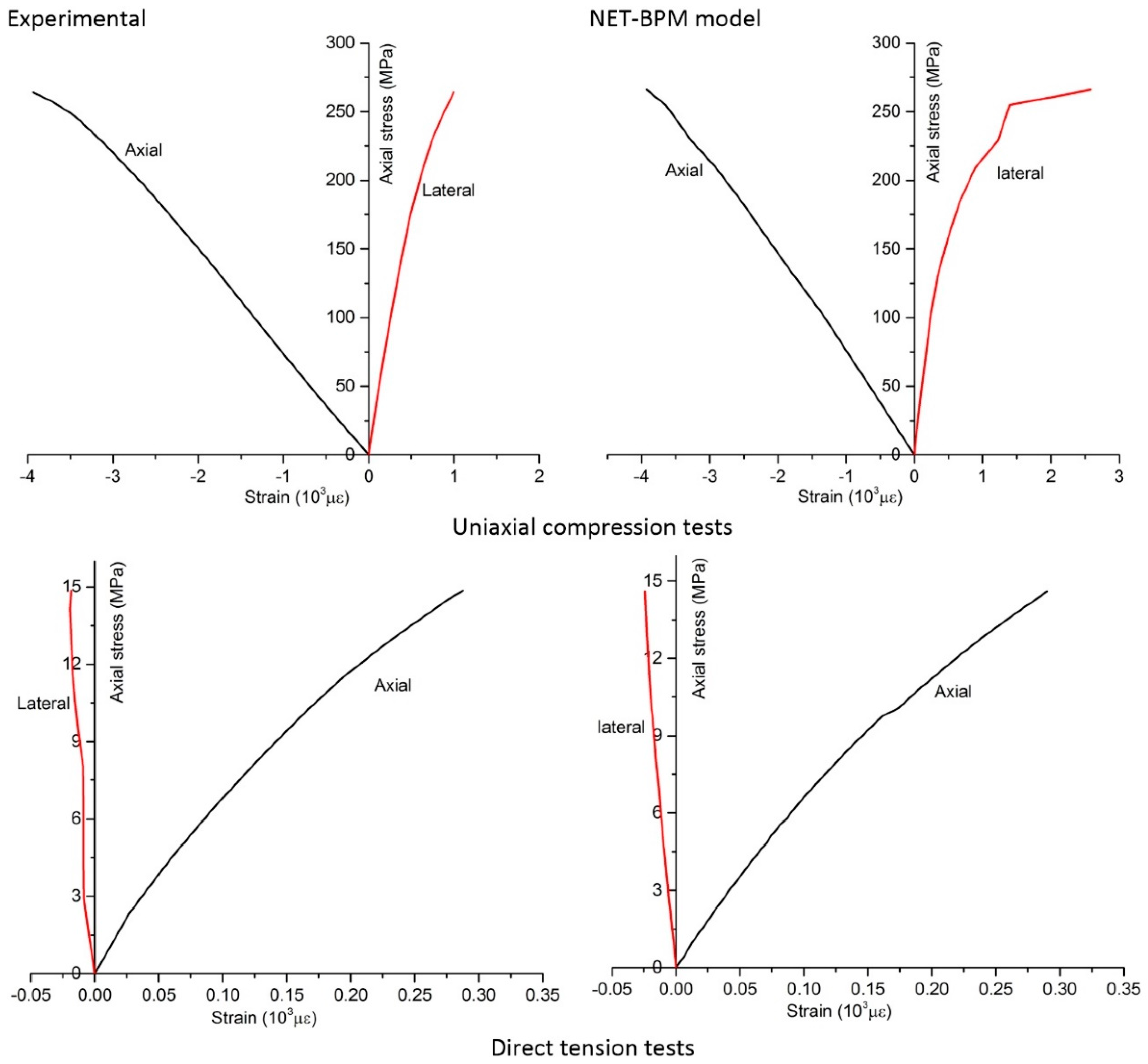
Figure 17.
Crack patterns of the Quartzite under compression and tension: (a) Compression at t = tcm; (b) Compression at t = tcm + 10,000∆t; (c) Compression at t = tcm + 20,000∆t; (d) Tension at t = ttm.
Figure 17.
Crack patterns of the Quartzite under compression and tension: (a) Compression at t = tcm; (b) Compression at t = tcm + 10,000∆t; (c) Compression at t = tcm + 20,000∆t; (d) Tension at t = ttm.

Table 1.
Parameters of the specimens.
| Specimens | Ra (mm) | Particle Number | Bonded Contacts | Porosity (%) | Overlap Ratio (10−15) |
|---|---|---|---|---|---|
| Specimen A | 0.544 | 2031 | 5100 | 13.77 | 5.4 |
| Specimen B | 0.559 | 2006 | 5031 | 13.76 | 4.9 |
| Specimen C | 0.557 | 2023 | 5089 | 13.65 | 4.7 |
| Specimen D | 0.560 | 1996 | 5004 | 13.72 | 4.2 |
| Specimen E | 0.564 | 1960 | 4912 | 14.02 | 6.2 |
Table 2.
Values of the micro parameters in the model.
| (106 N) | ks/kn | km/(knR) | (10−3) | (°) | (°) | w | b | ||
|---|---|---|---|---|---|---|---|---|---|
| 30.0 | 0.5 | 0.256 | 4.0 | 3.5 | 10 | 45 | 39 | 0.8 | 0.2 |
Table 3.
Properties of specimens; UCS: uniaxial compressive strength; TS: tensile strength.
| Specimens | Ec (GPa) | Et (GPa) | vc | vt | UCS (MPa) | TS (MPa) | UCS/TS | Ec/Et | vc/vt |
|---|---|---|---|---|---|---|---|---|---|
| Specimen A | 16.9 | 14.4 | 0.19 | 0.11 | 185.0 | 11.4 | 16.2 | 1.17 | 1.69 |
| Specimen B | 16.9 | 15.4 | 0.19 | 0.14 | 195.2 | 9.5 | 20.5 | 1.10 | 1.29 |
| Specimen C | 17.4 | 13.8 | 0.20 | 0.13 | 206.4 | 13.0 | 15.9 | 1.26 | 1.58 |
| Specimen D | 15.0 | 12.5 | 0.19 | 0.11 | 164.1 | 11.3 | 14.5 | 1.20 | 1.64 |
| Specimen E | 16.7 | 13.0 | 0.21 | 0.13 | 194.9 | 14.6 | 13.4 | 1.29 | 1.69 |
| Average | 16.6 | 13.8 | 0.19 | 0.12 | 189.1 | 12.0 | 16.1 | 1.20 | 1.58 |
| Stand deviation | 0.81 | 1.02 | 0.01 | 0.01 | 14.24 | 1.71 | 2.43 | 0.07 | 0.15 |
Table 4.
Parameters of specimens for LDB (Lac du Bonnet) granite and the quartzite.
| Parameters | Size (mm) Width/Height | Ra (mm) | Particle Number | Bonded Contacts | Porosity (%) | Overlap Ratio (10−14) |
|---|---|---|---|---|---|---|
| LDB | 63/157.5 | 0.562 | 7892 | 20071 | 13.48 | 1.55 |
| Quartzite | 31/78 | 0.373 | 4365 | 11021 | 13.67 | 1.22 |
Table 5.
Properties of LDB granite and the quartzite from experiments and simulations.
| Properties | UCS (MPa) | TS (MPa) | UCS/TS | Ec (GPa) | Et (GPa) | Ec/Et | vc | |
|---|---|---|---|---|---|---|---|---|
| LDB granite | Experimental | 200.0 | 9.3 | 21.5 | 68.1 | 47.5 | 1.43 | 0.35 |
| NET-BPM | 201.4 | 9.3 | 21.7 | 68.0 | 46.8 | 1.45 | 0.36 | |
| Quartzite | Experimental | 264.0 | 14.9 | 17.8 | 75.3 | 66.6 | 1.13 | 0.20 |
| NET-BPM | 265.8 | 14.8 | 18.0 | 75.7 | 62.0 | 1.22 | 0.20 | |
Table 6.
Micro parameters in NET-BPM (nonlinear elastic tensile bonded particle model) for LDB granite and the quartzite.
Table 6.
Micro parameters in NET-BPM (nonlinear elastic tensile bonded particle model) for LDB granite and the quartzite.
| Parameters | (106 N) | ks/kn | km/(knR) | (10−3) | (°) | (°) | w | b | ||
|---|---|---|---|---|---|---|---|---|---|---|
| LDB | 127 | 0.37 | 0.24 | 1.10 | 4.36 | 10 | 45 | 39 | 0.8 | 0.095 |
| Quartzite | 87 | 0.50 | 0.32 | 0.72 | 7.18 | 10 | 45 | 39 | 0.8 | 0.300 |
© 2017 by the authors. Licensee MDPI, Basel, Switzerland. This article is an open access article distributed under the terms and conditions of the Creative Commons Attribution (CC BY) license (http://creativecommons.org/licenses/by/4.0/).
Share and Cite
MDPI and ACS Style
Ouyang, Y.; Yang, Q.; Chen, X. Bonded-Particle Model with Nonlinear Elastic Tensile Stiffness for Rock-Like Materials. Appl. Sci. 2017, 7, 686. https://doi.org/10.3390/app7070686
AMA Style
Ouyang Y, Yang Q, Chen X. Bonded-Particle Model with Nonlinear Elastic Tensile Stiffness for Rock-Like Materials. Applied Sciences. 2017; 7(7):686. https://doi.org/10.3390/app7070686
Chicago/Turabian StyleOuyang, Yiping, Qi Yang, and Xinquan Chen. 2017. "Bonded-Particle Model with Nonlinear Elastic Tensile Stiffness for Rock-Like Materials" Applied Sciences 7, no. 7: 686. https://doi.org/10.3390/app7070686
Note that from the first issue of 2016, this journal uses article numbers instead of page numbers. See further details here.