
The New Concept of Nano-Device Spectroscopy Based on Rabi–Bloch Oscillations for THz-Frequency Range

Department from Physical Electronics, School of Electrical Engineering, Tel Aviv University, Tel Aviv 39040, Israel
*
Author to whom correspondence should be addressed.
Appl. Sci. 2017, 7(7), 721; https://doi.org/10.3390/app7070721
Submission received: 21 June 2017
/
Revised: 9 July 2017
/
Accepted: 10 July 2017
/
Published: 14 July 2017
(This article belongs to the Special Issue Nanophotonics)
Abstract
:We considered one-dimensional quantum chains of two-level Fermi particles coupled via the tunneling driven both by ac and dc fields in the regimes of strong and ultrastrong coupling. The frequency of ac field is matched with the frequency of the quantum transition. Based on the fundamental principles of electrodynamics and quantum theory, we developed a general model of quantum dynamics for such interactions. We showed that the joint action of ac and dc fields leads to the strong mutual influence of Rabi- and Bloch oscillations, one to another. We focused on the regime of ultrastrong coupling, for which Bloch- and Rabi-frequencies are significant values of the frequency of interband transition. The Hamiltonian was solved numerically, with account of anti-resonant terms. It manifests by the appearance of a great number of narrow high-amplitude resonant lines in the spectra of tunneling current and dipole moment. We proposed the new concept of terahertz (THz) spectroscopy, which is promising for different applications in future nanoelectronics and nano-photonics.
1. Introduction
Since the early days of physics, spectroscopy has been a platform for many fundamental investigations. One of the central concepts in spectroscopy is a resonance, with its corresponding resonant frequency. Types of spectroscopy can also be distinguished by the nature of the interaction between the electromagnetic field (EM-field) and the condensed matter (as examples, one may mention absorption and emission of light, Raman and Compton scattering, nuclear magnetic resonance, etc.). The first period in the development of spectroscopy is associated with atomic and molecular spectroscopy. Atoms of different elements have distinct spectra, and therefore, atomic spectroscopy allows for the identification of a sample’s elemental composition. The spectral lines obtained by experiment and theory can be mapped to the Mendeleev Periodic Table of the Elements. Spectroscopic studies at this time, were central to the development of quantum mechanics.
The second period in the making of spectroscopy is associated with a wide range of applications to different types of chemical substances: gases, liquids, crystals, polymers, etc. The combination of atoms or molecules into macroscopic samples leads to the creation of many-particle quantum states, whereby different materials have distinct spectra. Therefore, spectroscopy observations in a wide frequency range (from microwave until gamma-ray) became an irreplaceable tool for the identification of a sample’s structure, chemical composition, quality, etc. in material engineering, physical chemistry, and biophysics. Recent progress in electronics and informatics is associated with the development of nanotechnologies and synthesis of different types of nano-objects. The distinct spectra became the attribute of nano-objects of various spatial configurations, but the same chemical composition. In this context, the future of spectroscopy development would probably be associated with the spectroscopy of a whole range of electronic devices, or their rather large components. This trend will provide tools of the tunable spectroscopy adapted for such types of tasks. The promising examples from this point of view are based on the strong and ultrastrong interactions of condensed matter with EM-field.
The strong-coupling field–matter interaction is defined as a regime, in which the EM-field does not correspond to the small perturbation [1]. It leads to the periodical transitions of a two-level quantum system between its stationary states under the action of ac driving field (Rabi-oscillations—RO) [1]. The phenomenon was theoretically predicted by Rabi on nuclear spins in radio-frequency magnetic field [2], and afterwards, discovered in various physical systems, such as electromagnetically driven atoms [3], semiconductor quantum dots [4], and different types of solid-state qubits [5,6,7,8,9]. The simplest physical picture of the Rabi effect is given by the model of a single atom [1]. It can be essentially modified by a set of additional features, such as broken inversion symmetry [10], spatial RO propagation in the arrays of coupled Rabi-oscillators (Rabi-waves), and local field depolarization effects [11,12,13,14,15,16].
The early quantum theory of electrical conductivity in crystal lattices by Bloch, Zener and Wannier [17,18,19,20], led to the prediction that a homogeneous dc field induces an oscillatory, rather than uniform, motion of the electrons. These so-called Bloch-oscillations (BO) have never been observed in natural crystals because the scattering time of the electrons by the lattice defects is much shorter than the Bloch period [21]. In semiconductor superlattices, the larger spatial period leads to a much shorter Bloch period, and BO have been observed through the THz radiation of the electrons [22]. BO in dc biased lattices is due to wave interference, and have been observed in a number of quite different physical systems: a few interacting atoms in optical lattices [23,24], ultracold atoms [25,26,27,28,29,30], light intensity oscillations in waveguide arrays [31,32,33,34,35,36,37], acoustic waves in layered and elastic structures [38], atomic oscillations in Bose-Einstein condensates [39], among others. Several recent studies have investigated the dynamics of cold atoms in optical lattices subject to ac forcing; the theoretically predicted renormalization of the tunneling amplitudes has been verified experimentally. Recent observations include global motion of the atom cloud, such as giant “super-Bloch oscillations” [40]. As a result, BO was transformed from a partial physical effect, to the universal phenomenon of oscillatory motion of wave packets placed in a periodic potential, when driven by a constant force [24,41].
Recently, there have been several theoretical studies of the ultrastrong light–matter interaction regime [42,43,44,45], where the Rabi frequency becomes comparable with the frequency of the inter-zone quantum transition [43]. This regime has been realized experimentally with intersubband transitions coupled with plasmon waveguides in the infrared frequency range [46], and metallic microcavities in the THz [47,48,49], magnetoplasmons of two-dimensional electron gas [50], superconducting qubits [51], and molecular transitions [52]. It was shown that the system behaves like a multi-level quantum bit with non-monochromatic energy spacing, owing to the inter-particle interactions.
One of the general tendencies in modern physics consists of the synthesis of different physical mechanisms in the network of one physical process, with their strong mutual influence. One of such examples have been demonstrated in [53], where the quantum chain of the coupled two-level fermion systems driven simultaneously by ac and dc fields was considered. It was shown that in the case of resonant interaction with an ac-component, the particle dynamics exhibits itself in the oscillatory regime, which may be interpreted as a combination of RO and BO, with their strong mutual influence. This type of quantum dynamics was named in [53] as Rabi–Bloch oscillations (RBO). Such a scenario dramatically differs from the individual picture of both types of oscillations due to the interactions. This novel effect is counterintuitive because of the strongly different frequency ranges for two such types of oscillation existences.
In this paper, we consider the RBO in the regimes of strong and ultrastrong coupling. We present the approximate analytical solution, and results of the numerical modelling. We study both the temporal dynamics and spectra, identify the spectral lines, and compare the spectra behavior in the strong and ultrastrong regimes. Conclusively, we discuss the promising applications of our results in the novel types of spectroscopy.
2. Structures and Models
The model system for RBO observation in the strong coupling regime is shown in Figure 1. It corresponds to the periodic two-level atomic chain, excited with an obliquely incident ac field in the strong coupling regime, and driven with dc voltage applied at the ends. The neighboring atoms are coupled via interatomic tunneling, with different values of penetration at the ground and excited states.
The model system for RBO analysis in the ultrastrong coupling regime is shown in Figure 2. Analysis of RO in the regime of ultrastrong coupling was given in [43], performing on a model system depicted in Figure 2a, where a mode of microcavity of THz frequency range is coupled with the electronic excitation of a highly doped quantum well (QW) inserted inside the capacitor. There are at least two confined subbands in the QW, and the fundamental subband hosts a two-dimensional electron gas with an arbitrary total number of electrons. The energy difference between the first and the second subband is matched with the resonance of the LC circuit. The reduction of the capacitor armatures also implies a reduction of the capacitance C, which in turn changes the resonant frequency of the LC circuit. In order to keep the resonator frequency always matched with the frequency of the quantum transition, one has to increase the inductance, L. The strong reduction of the capacitor volume in the quantum LC resonator allows for the realization of the ultrastrong coupling regime with a few electrons only, even with a single electron. It was focused in [43] on the case of an electron gas coupled with the circuit photons of the capacitor. One of the peculiar features of such a quantum mechanical system is the existence of entangled light–matter excitations in analogy with the super-radiant and sub-radiant Dicke states in atomic clouds [43].
The system under consideration in our case, is in essence, different. We consider the periodic chain of elements [43], every one of which plays the role of the single atom in Figure 1. The chain is driven by both dc and classical THz frequency field (Figure 2b). The THz oscillating voltage is applied to the system through a nano-antenna [54,55,56,57,58,59,60,61,62,63] (Figure 2b). The QW is assumed to be periodically doped, thus the additional periodic potential has been induced (Figure 2c). We assume only one electron in the system. The coupling is governed by the inter-barrier electron tunneling. In our case, QW represents the effective super-lattice, which is able to support the electron’s BO [21] and was the first system in which BO was experimentally observed [21,41].
Of course, these two models are identical from a physical point of view. The difference is only in the reachable value of the coupling factor, which makes the contribution of anti-resonant terms significant. These models relate to the different frequency ranges (optical—Figure 1, THz—Figure 2). As it leads from analysis [43], the ultrastrong coupling becomes implementable in THz, while remains open in optics. Thus, the optical model will be simplified via RWA, while the THz one is based on the total Hamiltonian.
We use for analysis, the method of probability amplitudes [1]. The single-electron motion is described by the wave function and satisfies the Schrodinger equation, , where is the total Hamiltonian of the system. The Hamiltonian may be decomposed as , where is the component of free electron movement in the chain associated with the tunneling, and described by the periodic superlattice potential (Figure 2c). The second component , corresponds to the interaction of electron with total (dc and ac) EM-field. The electron interaction with EM-field is described in the dipole approximation [1], thus , where is the operator of electron position in the chain, and is the superposition of dc and ac components. Our analysis will based on the Wannier basis [17,18,19,20]; the presentation of Hamiltonian in the Wannier basis is given in [53].
3. Strong Coupling Regime: Analytical Approximation
The wave function for the single-particle state of Hamiltonian is given by:
where are Wannier functions of the atom with number p in the excited and ground states, respectively [53], and the unknown variables, which are satisfy the system differential equations:
In this section, we will consider Equations (2) and (3) analytically, assuming for simplicity that the exact resonance condition is fulfilled ().
3.1. Travelling Rabi-Waves
Assuming the driven dc field to be absent (), we have from (2) and (3):
The idea of simplifying Equations (4) and (5) is based on the so-called rotating-wave approximation (RWA), which is frequently encountered in quantum optics [1]. It takes into account only the co-rotating field with the system, and neglects the counter-rotating part, which is proportional to [1]. This part oscillates very rapidly, and its average over the time larger than is zero, if (strong coupling regime). It corresponds to the exchanges , , and leads to the equations:
For and have been comparable, the average of the counter-rotating part does not vanish due to the high amplitude of such rapid oscillations (ultra-strong coupling). The equations of motion, in contrast with the system (6) and (7), become analytically unsolvable and should be integrated numerically. The system (6) and (7) is a generalization of Jaynes–Cummings model for the single atom to the case of atomic chain.
The ansatz for solutions of Equations (6) and (7) in the form of a travelling wave is
where are unknown coefficients, is the phase shift per unit cell, is the eigen frequency. Substituting (6)–(8), we obtain the system with respect to :
Setting determinant equal to zero, we obtain the characteristic equation with respect to :
with two solutions:
The linearly independent eigen modes correspondent to eigen frequencies (11) are:
where is a number of atoms in the chain and
The general solution for Rabi-oscillations propagated along the chain in the form of travelling waves is given by the linear superposition of eigen modes (12), (13) , where are arbitrary integration constants. Using Equations (12) and (13), it may be transformed to
where , and
The constants satisfy the normalization condition , (guarantee the correct normalization for the wavefunction (15)). Let us assume the system initially prepared in the excited state (). In this case, we obtain from (16) and (17):
where the RO frequency is given by
It is important to note that it is corrected with respect to Rabi-frequency, due to the interatomic coupling via tunneling.
3.2. Tunneling Current
Following the general presentation of tunneling current in terms of probability amplitudes [1], we have for RO
For the case of a completely excited initial state, we obtain using (18) and (19):
In this case, the tunnel current consists of two components: dc-current, and the component on the RO frequency (20). Its physical origin is similar to the so-called low-frequency RO in the two-level quantum systems with broken inversion symmetry [10]. As was predicted in [10], it leads to non-zero diagonal matrix elements of dipole moment. It is impossible for real atoms (excluding hydrogen), but implementable for artificial atoms (for example, self-organized semiconductor quantum dots). As a result, the inter-level optical transitions are accompanied by the intra-level periodical movement with Rabi-frequency, which is responsible for low-frequency radiation. It exists only in the case of asymmetry, which manifests itself in the non-identity of diagonal dipole matrix elements. In our case, the intra-band movement and correspondent asymmetry are associated with interatomic tunneling and different penetration values (), respectively.
3.3. Rabi–Bloch Oscillations: Quasiclassical Model
BO of the charge particles is a pure quantum effect which can be explained in a simple quasiclassical model [21,24,25]. The similar concept may be developed for quasi-particles (Rabi-oscillated electrons in our case). The periodicity of the lattice leads to a band structure of the energy spectrum and the corresponding eigen energies given by Equation (11). The eigen states given by Equations (12) and (13), are labeled by the continuous quasimomentum h; and are periodic functions of h with period , and h is conventionally restricted to the first Brillouin zone . Under the influence of dc field, weak enough not to induce interband transitions, a given state evolves up to a phase factor into the state , with variation according to
or . Thus, this evolution is periodic with a Bloch frequency corresponding to the time required for the quasimomentum to scan a full Brillouin zone. It leads to the exchanges
where .
Equations (24)–(26) allow the spectrum of the tunneling current in the BO regime to be analyzed. Following quasiclassical concepts, the tunneling current may be considered as RO, with modulated amplitude and frequency. As it leads from Equations (24)–(26), the spectral presentation of tunnel current is given by
where and are the spectral amplitudes. Below, we consider the amplitude relations in the current spectra based on the numerical solution of motion equations. Here, we note that the small detuning for which , with , is associated with a special type of resonance motion. The above represents a superposition of harmonic oscillations, which evolves slowly in time, with a period , where are the Rabi and Bloch periods, respectively. Evaluating the particle position as , we obtain It shows the strong enhancement of spatial oscillations, which is similar to the super-Bloch oscillations recently predicted and experimentally observed in optical lattices with cold atoms [40]. In contrast with super-Bloch oscillations, in our case, there exists two tunneling channels (with respect to the different zones). Thus, the influence of ac field does not add up to renormalization of tunneling factors, but leads to their mutual influence via Rabi-oscillations.
4. Ultrastrong Coupling: Results and Discussion
In this section, we will consider the dynamics and spectra for the case of ultrastrong coupling. As was mentioned above, the equations of motion are analytically unsolvable, and were integrated numerically with the technique [64].
4.1. The Case of Small Bloch-Frequency
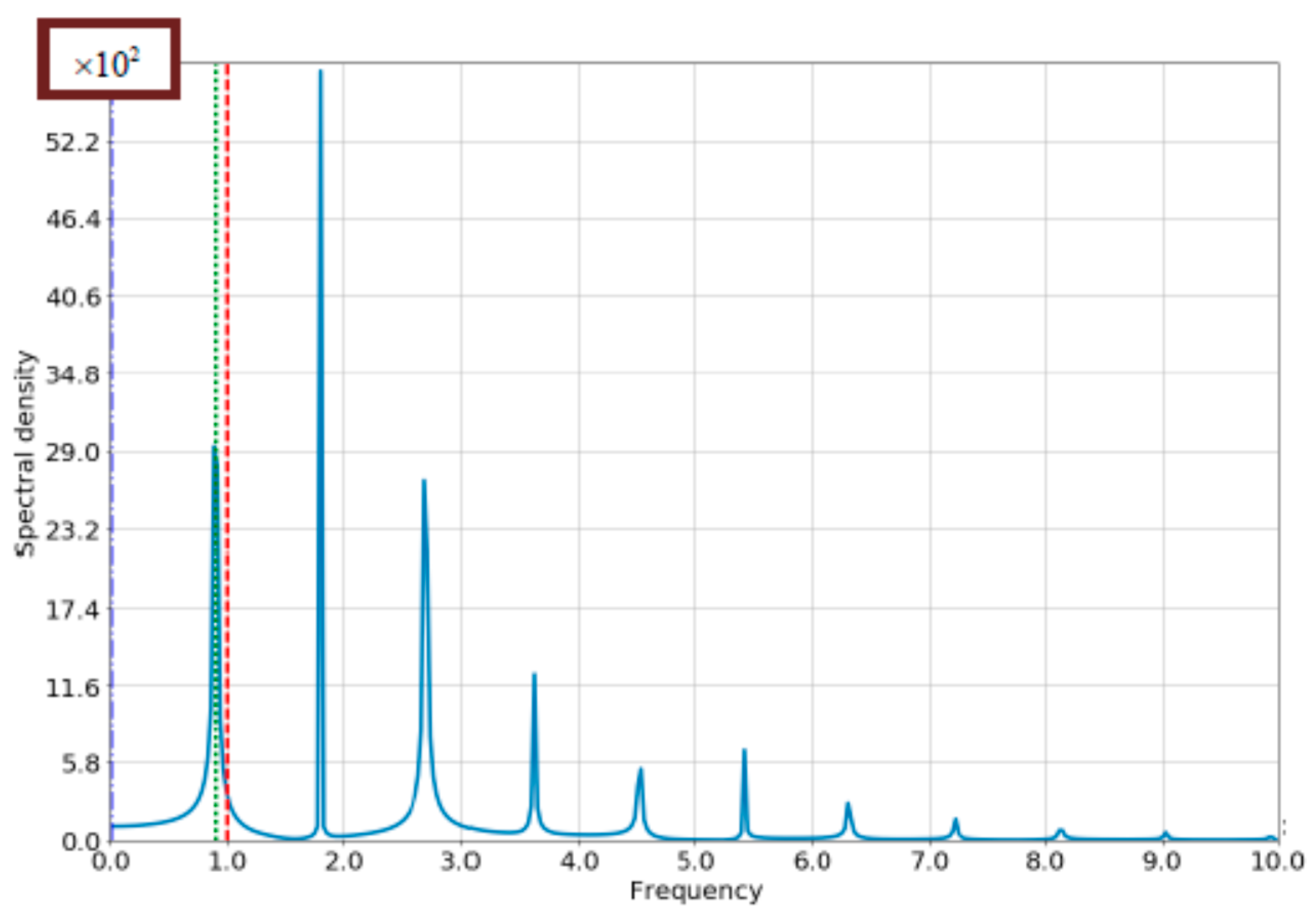
In this subsection, we consider the case of Rabi-frequency comparable with the quantum transition frequency, but strongly exceeding Bloch-frequency (, while ). The spatial–temporal behavior of the tunnel current, for different types of relative values of tunneling factors at ground and excited states, is presented in Figure 3 and Figure 4. The current oscillates with Bloch frequency. The amplitude for the case exceeds the case . The current amplitude is high frequency modulated. In general, the scenario looks like as in the case of strong coupling.
In Figure 5 and Figure 6, the corresponding spectra are presented. Their qualitative behavior dramatically changes with respect to the strong coupling regime (see Equation (27)). The main reason leads from the strong analysis of the system in Equations (2) and (3), which is free from RWA, and based on Floquet theorem. Following it, the probability amplitudes of the j-th mode are presented in the form
where are the periodical functions of the phase shift per unit cell, and is the eigen value. Therefore, as it leads from Equation (21), the lines appear at the frequency spectrum, and the first of them are really observed at Figure 5 and Figure 6, in contrast with relation (27). Following the quasiclassical approach, we exchange , thus the values become time dependent periodic functions with a Bloch-period. Such amplitude modulation means the appearance of lines , where . The frequency-modulated factors , for qualitative analysis, may be averaged over the Bloch-period [40]. The dominant support to observable values is defined by two first modes, with j = 1,2. Thus, the discrete part of the spectra in the regime of ultrastrong coupling corresponds to the narrow lines with the frequencies
where , and
This frequency may be identified with the frequency of RO. The spectrum defined by Equation (29) corresponds to the physical picture of RBO as a superposition of three partial motions: (i) a single quantum transition from the ground to excited state (or vice versa); (ii) the series of periodic quantum transitions between different states with frequency (RO); (iii) the spatial oscillations as a comprehensive whole, with frequency (BO). Of course, the validity of this picture is essentially strongly limited, in view of the fact that the travelling waves are used as a model of excitation. But if we go to the wavepacket with strongly defined momentum, this picture will be adequate too, and is supported by the numerical calculations presented below. The similar general scenario of the complex dynamics manifests itself in a lot of other physical systems. In particular, as one more example, the coherent control of charge fluxes in unbiased molecular junctions may be considered, and is discussed in [65]. Such control is induced by resonances between the Rabi-oscillations driven by a pumping laser field, and the bridge mediated tunneling oscillations between the lowest unoccupied molecular orbitals of the donor and acceptor. One can see that the resonance condition [65] corresponds to Equation (29) for . The frequency given by Equation (30) is associated with the Rabi frequency in [64]. The frequency of intra-molecular oscillations driven by the donor–acceptor tunneling in [65] may be identified as a Bloch frequency in Equation (29).
We will comment only on the analysis and physical interpretation of the dominative lines, which will keep their resolvability in real experimental conditions. The spectra in Figure 5 and Figure 6 are clearly separated into low-frequency and high-frequency regions. The low-frequency part consists of the single line , while the high-frequency part consists of the different sub-harmonics (29). The low-frequency part corresponds to the ordinary BO; the high frequency spectrum is governed by the RO. The dipole moment and inversion densities are presented in Figure 7 and Figure 8, and corresponding spectra in Figure 9 and Figure 10, respectively.
As one can see, the dipole current and inversion densities are modulated by the Bloch frequency. The reason is the mutual influence of BO and RO. The low frequency component corresponds to the mutual influence of RO and BO in the so-called RBO regime.
4.2. The Case of Comparable Rabi- and Bloch Frequencies
In this subsection, we consider another case: when the Rabi- and Bloch frequencies are comparable (Figure 11 and Figure 12). The scenario dramatically changes; the total spectrum is not separable into low-frequency and high-frequency components. As one can see in Figure 12, there is the appearance of the combined sub-harmonics of Bloch and Rabi-frequencies, according to Equation (27) (RBO regime).
In Figure 13 and Figure 14, the spectra of tunneling current and dipole moment densities for are presented. In this special case, a lot of sub-harmonics become degenerate. As a result, the density of spectral lines decreases and the ability of their resolution in real experiments grows, avoiding a strong overlap via dissipative broadening. Appearing are the lines (see Figure 14), at first, it appears they may be associated with a Mollow triplet, but no rather convincing arguments for such an interpretation exist. The reason is the degeneracy of the modes of different origins in our case, in contrast with Lorentz single-oscillator lines in Mollow triplets [1].
4.3. The Role of the Losses
One of distinctive features of ultrastrong coupling is a comparable value of inter-band transition with radiative and dissipative damping value. Thus, the dissipative and radiative broadening leads to the confluence of neighboring spectral lines. As a result, the discrete lines will interchange with areas of continuous spectra. These discrete lines will have non-Lorentz asymmetric form. This means that the simple lossless model is not applicable for detailed analysis of the spectra thin structure—it allows only prediction of the spectral line positions and their relative amplitudes. For estimating the role of losses, we will use the simple phenomenological model used by Scully et al., for the analysis of population trapping, lasing without inversion, and electromagnetically induced transparency [1]. This model assumes that two levels decay at a rate [1,66]. This means that the ground state is not really ground, and corresponds to the excited state at the lowest energy level. The wavefunction for such model is given by
where are the same coefficients as in the lossless system.
The tunneling current and its frequency spectrum for Q = 15 are shown in Figure 15 and Figure 16. One can see that the oscillation process quickly reduces (Figure 15). The number of the resolved spectral lines decreases with decay appearance (Figure 16), because of the large number of lines run into, due to the broadening. The main lines are kept, however, their positions are shifted and amplitudes are decreased with respect to the lossless case. The frequency spectrum of the tunneling current for is shown in Figure 17. The mechanism of the spectral lines confluence due to the losses, is especially well-defined in this partial case via the transformation of duplets to their corresponding broadened singlets. The non-Lorentz origin of these spectral lines manifests itself in their asymmetry. Such qualitative behavior agrees with general principles of the oscillations’ theory [67]. The detailed description of losses must be based on the concept of open quantum systems [68], and master equation technique especially adopted to the case of ultrastrong coupling [69]. It goes beyond the subject of this article, and may be one of the topics for future research activity.
Another topic for future activity is the implementation of the scenario considered before. The subject of this article is limited by the guidance of some candidates for such potential experiments. As one example, the multi-exciton dynamics in the linear chain of identical molecules with transition dipole moment perpendicular to the chain axis (H-aggregate configuration) [70], may be marked. The number of emitters in [70] is , the distance nm, meV, and ns. The reachable values of the ac field V/m for the frequencies eV noted in [70] correspond to the strong coupling regime. The agreed values are implementable for the chain of 1D semiconductor quantum dots [14], which makes it another candidate for RBO experiments in the strong coupling regime. The suitable structure for RBO ultrastrong coupling was implemented via plasmon polaritons in parabolic semiconductor quantum wells [71]. The electronic feedback microcavity was composed of circular capacitor elements connected via the wires of finite inductance. The cavity has been tuned by changing the electrical size of the components. A parabolic potential was approximated by digitally alloying layers. The well has been surrounded by barriers, containing Si- doping. The use of parabolic quantum wells enabled very large values of the ratio of for THz frequency range ( = 0.205 for the lower doped sample and = 0.27 for the heavier doped one) to be achieved in [71].
4.4. Stark Effect in One-Dimensional Atomic Chains
In this section, we consider the 1D chain of two-level atoms driven by dc field only. For a single atom, the interaction with a dc field leads to the well-known Stark effect, which consists of the shifting of energy levels [48]. For reachable field values, the shift is small, and considered as a perturbation of the energy spectrum (weak coupling regime) [48]. The dc field couples all eigen states of the atom, thus the multi-level model with summation over the complete set of atomic terms is applicable to real atoms. Here, we show that the Stark effect manifests itself in 1D chains too, but its qualitative picture differs from the single-atomic case. The main reason is the performance ability of ultrastrong coupling, on which we focus below. The system under consideration is shown in Figure 18. The dipole moments of the atoms is assumed to be oriented orthogonally to the chain axis, and the dc field is directe d under the angle , with respect to the axis.
The analytical model, in general, is similar to the RBO-model developed and used before. The wave function is given by
where the probability amplitudes satisfy the system
where , , are the Rabi- and Bloch frequencies, respectively. In contrast with RBO, these two frequencies are defined by the same field (dc), but their relative values may be arbitrary, via the corresponding choice of the field direction (angle).
Let us assume that
and
Equation (35) corresponds to the resonant condition. It is a counterintuitive resonance, which does not couple with any oscillating forces, and represents the attribute of a ultrastrong coupling regime. This resonance legitimates the using of a two-level model, in contrast with the single-atomic case. This inequality (36) means high amplitude of BO. It allows us to separate the inter-atomic and intra-atomic motions, and describe the last one in terms of quasiclassical approximation. The wave function of inter-atomic motion is given as a superposition of eigen states (12) and (13). The account of intra-atomic motion is made via exchange (24). As a result, the total motion is described by the wave function (15) with
The application of this solution in relation to tunneling current (21) leads to the spectrum (29), in the case of Stark effect.
Another approach consists in the numerical solution of Equations (33) and (34), which is simplified by the absence of oscillation coefficients. The typical behavior of space–time distribution of inversions and tunneling currents, as well as the frequency spectrum of tunneling currents, are shown in Figure 19, Figure 20 and Figure 21. The scenario of the process may be explained in the following way: the ordinary Stark effect for the single atom consists in the perturbed energy spectrum and mixing of states due to the dc field [48]. In our case, the situation is similar, however, the energy shifting is not small. The system is initially prepared in the case of non-perturbed states, which is not related to the eigen modes of the system with the dc field applied. As a result, the new eigen modes become coupled, and we observe their mutual oscillations in inversion with Rabi-frequency (see Figure 19). These oscillations propagate along the chain with Rabi-period, due to the tunneling, and produce the intra-zone current (Figure 20). The value of this current strongly increases due to the resonant condition (35). The spectrum of this current is a set of lines , n = 1,2, … (see Figure 21). In the opposite case (dc field directed predominately along the chain), the inter-zone coupling becomes small, which leads to the suppression of intra-atomic motion. Thus, the total motion adds up to the oscillatory inter-atomic tunneling, which corresponds to the ordinary BO.
5. Conclusions
In summary, we developed the physical model of 1D two-level atomic chain, with the tunneling inter-atomic coupling simultaneously driven by dc and ac fields in the regimes of strong and ultrastrong coupling. The approximate analytical solutions and results of computer modeling of Rabi-Bloch oscillations have been presented and discussed. There is also considered limited cases, such as the Stark effect, Rabi-waves, and Bloch oscillations. The temporal dynamics, as well as the frequency spectra of tunneling currents, have been presented. It was shown that the passage to ultrastrong coupling dramatically changes the scenario of Rabi–Bloch oscillations. This manifests in the appearance of additional lines in the spectra of the tunneling current. These lines are identified as a contribution of anti-resonant interactions, and remain even in the case of high losses characteristic of ultrastrong coupling. The promising potential applications of the obtained results in novel types of THz spectroscopy for nano-electronics have been proposed.
Acknowledgments
Gregory Slepyan acknowledges support from the project FP7-PEOPLE-2013-IRSES-612285 CANTOR.
Author Contributions
Developments of the physical models, derivation of the basis equations, interpretation of the physical results and righting the paper have been done by Ilay Levie and Gregory Slepyan jointly. The MATHEMATICA Numerical Python calculations and figures were produced by Ilay Levie.
Conflicts of Interest
The authors declare no conflict of interest.
References
- Scully, M.O.; Zubairy, M.S. Quantum Optics; Cambridge University Press: Cambridge, UK, 2001. [Google Scholar]
- Rabi, I.I. Space Quantization in a Gyrating Magnetic Field. Phys. Rev. 1937, 51. [Google Scholar] [CrossRef]
- Hocker, G.B.; Tang, C.L. Observation of the Optical Transient Nutation Effect. Phys. Rev. Lett. 1968, 21. [Google Scholar] [CrossRef]
- Kamada, H.; Gotoh, U.; Temmyo, J.; Takagahara, T.; Ando, H. Exciton Rabi Oscillation in a Single Quantum Dot. Phys. Rev. Lett. 2001, 87. [Google Scholar] [CrossRef] [PubMed]
- Blais, A.; Huang, R.S.; Wallraff, A.; Girvin, S.M.; Schoelkopf, R.J. Cavity quantum electrodynamics for superconducting electrical circuits: An architecture for quantum computation. Phys. Rev. A 2004, 69. [Google Scholar] [CrossRef]
- Gambetta, J.; Blais, A.; Schuster, D.I.; Wallraff, A.; Frunzio, L.; Majer, J.; Devoret, M.H.; Girvin, S.M.; Schoelkopf, R.J. Qubit-photon interactions in a cavity: Measurement-induced dephasing and number splitting. Phys. Rev. A 2006, 74. [Google Scholar] [CrossRef]
- Blais, A.; Gambetta, J.; Wallraff, A.; Schuster, D.I.; Girvin, S.M.; Devoret, M.H.; Schoelkopf, R.J. Quantum-information processing with circuit quantum electrodynamics. Phys. Rev. A 2007, 75. [Google Scholar] [CrossRef]
- Burkard, G.; Imamoglu, A. Ultra-long-distance interaction between spin qubits. Phys. Rev. B 2006, 74. [Google Scholar] [CrossRef]
- Barrett, S.D.; Milburn, G.J. Measuring the decoherence rate in a semiconductor charge qubit. Phys. Rev. B 2003, 68, 155307. [Google Scholar] [CrossRef]
- Kibis, O.V.; Slepyan, G.Y.; Maksimenko, S.A.; Hoffmann, A. Matter Coupling to Strong Electromagnetic Fields in Two-Level Quantum Systems with Broken Inversion Symmetry. Phys. Rev. Lett. 2009, 102, 023601. [Google Scholar] [CrossRef] [PubMed]
- Slepyan, G.Y.; Yerchak, Y.D.; Maksimenko, S.A.; Hoffmann, A. Wave propagation of Rabi oscillations in one-dimensional quantum dot chain. Phys. Lett. A 2009, 373, 1374–1378. [Google Scholar] [CrossRef]
- Slepyan, G.Y.; Yerchak, Y.D.; Maksimenko, S.A.; Hoffmann, A.; Bass, F.G. Mixed states in Rabi waves and quantum nanoantennas. Phys. Rev. B 2012, 85. [Google Scholar] [CrossRef]
- Yerchak, Y.; Slepyan, G.Y.; Maksimenko, S.A.; Hoffmann, A.; Bass, F. Array of tunneling-coupled quantum dots as a terahertz range quantum nanoantenna. J. Nanophotonics 2013, 7. [Google Scholar] [CrossRef]
- Slepyan, G.Y.; Yerchak, Y.D.; Hoffmann, A.; Bass, F.G. Strong electron-photon coupling in a one-dimensional quantum dot chain: Rabi waves and Rabi wave packets. Phys. Rev. B 2010, 81. [Google Scholar] [CrossRef]
- Gligorić, G.; Maluckov, A.; Hadžievski, L.; Slepyan, G.Y.; Malomed, B.A. Discrete solitons in an array of quantum dots. Phys. Rev. B 2013, 88. [Google Scholar] [CrossRef]
- Gligorić, G.; Maluckov, A.; Hadžievski, L.; Slepyan, G.Y.; Malomed, B.A. Soliton nanoantennas in two-dimensional arrays of quantum dots. J. Phys. 2015, 27. [Google Scholar] [CrossRef] [PubMed]
- Bloch, F. UЁ ber die Quantenmechanik der Elektronen in Kristallgittern. Z. Phys. 1929, 52, 555–600. [Google Scholar] [CrossRef]
- Zener, C.A. Theory of electrical breakdown of solid dielectrics. Proc. R. Soc. Lond. A 1934, 145, 523–529. [Google Scholar] [CrossRef]
- Wannier, G.H. Wave functions and effective Hamiltonian for Bloch electrons in an electric field. Phys. Rev. 1960, 117. [Google Scholar] [CrossRef]
- Wannier, G.H. Stark ladder in solids? A reply. Phys. Rev. 1969, 181. [Google Scholar] [CrossRef]
- Duan, F.; Guojin, J. Introduction to Condensed Matter Physics; World Scientific: Hackensack, NJ, USA, 2007. [Google Scholar]
- Waschke, C.; Roskos, H.; Schwedler, R.; Leo, K.; Kurz, H.; Köhler, K. Coherent submillimeter-wave emission from Bloch oscillations in a semiconductor superlattice. Phys. Rev. Lett. 1993, 70, 3319–3322. [Google Scholar] [CrossRef] [PubMed]
- Preiss, P.M.; Ma, R.; Tai, M.E.; Lukin, A.; Rispoli, M.; Zupanic, P.; Lahini, Y.; Islam, R.; Greiner, M. Strongly correlated quantum walks in optical lattices. Science 2015, 347, 1229–1233. [Google Scholar] [CrossRef] [PubMed]
- Gluck, M.; Kolovsky, A.R.; Korsch, H.J. Wannier–Stark resonances in optical and semiconductor superlattices. Phys. Rep. 2002, 366, 103–182. [Google Scholar] [CrossRef]
- Dahan, M.B.; Peik, E.; Reichel, J.; Castin, Y.; Salomon, C. Bloch Oscillations of Atoms in an Optical Potential. Phys. Rev. Lett. 1996, 76, 4508–4511. [Google Scholar] [CrossRef] [PubMed]
- Madison, K.W.; Fischer, M.C.; Diener, R.B.; Niu, Q.; Raizen, M.G. Dynamical Bloch Band Suppression in an Optical Lattice. Phys. Rev. Lett. 1998, 81, 5093–5096. [Google Scholar] [CrossRef]
- Morsch, O.; Muller, J.H.; Cristiani, M.; Ciampini, D.; Arimondo, E. Bloch Oscillations and Mean-Field Effects of Bose-Einstein Condensates in 1D Optical Lattices. Phys. Rev. Lett. 2001, 87, 140402–140410. [Google Scholar] [CrossRef] [PubMed]
- Bongs, K.; Sengstock, K. Physics with Coherent Matter Waves. Rep. Prog. Phys. 2004, 67, 907–963. [Google Scholar] [CrossRef]
- Ferrari, G.; Poli, N.; Sorrentino, F.; Tino, G.M. Long-Lived Bloch Oscillations with Bosonic Sr Atoms and Application to Gravity Measurement at the Micrometer Scale. Phys. Rev. Lett. 2006, 97. [Google Scholar] [CrossRef] [PubMed]
- Battesti, R.; Cladé, P.; Guellati-Khélifa, S.; Schwob, C.; Grémaud, B.; Nez, F.; Julien, L.; Biraben, F. Bloch Oscillations of Ultracold Atoms: A Tool for a Metrological Determination of h/mRb. Phys. Rev. Lett. 2004, 92, 253001–253005. [Google Scholar] [CrossRef] [PubMed]
- Morandotti, R.; Peschel, U.; Aitchison, J.S.; Eisenberg, H.S.; Silberberg, Y. Experimental Observation of Linear and Nonlinear Optical Bloch Oscillations. Phys. Rev. Lett. 1999, 83, 4756–4759. [Google Scholar] [CrossRef]
- Pertsch, T.; Dannberg, P.; Elflein, W.; Bräuer, A.; Lederer, F. Optical Bloch Oscillations in Temperature Tuned Waveguide Arrays. Phys. Rev. Lett. 1999, 83, 4752–4755. [Google Scholar] [CrossRef]
- Peschel, U.; Pertsch, T.; Lederer, F. Optical Bloch oscillations in waveguide arrays. Opt. Lett. 1998, 23, 1701–1703. [Google Scholar] [CrossRef] [PubMed]
- Agarwal, G.S. Quantum Optics; Cambridge University Press: Cambridge, UK, 2013. [Google Scholar]
- Bromberg, Y.; Lahini, Y.; Silberberg, Y. Bloch Oscillations of Path-Entangled Photons. Phys. Rev. Lett. (E) 2011, 105. [Google Scholar] [CrossRef] [PubMed]
- Afek, I.; Natan, A.; Ambar, O.; Silberberg, Y. Quantum state measurements using multipixel photon detectors. Phys. Rev. A 2009, 79. [Google Scholar] [CrossRef]
- Afek, I.; Ambar, O.; Silberberg, Y. High-NOON States by Mixing Quantum and Classical Light. Science 2010, 328, 879–881. [Google Scholar] [CrossRef] [PubMed]
- Sanchis-Alepuz, H.; Kosevich, Y.A.; Sanchez-Dehesa, J. Acoustic Analogue of Electronic Bloch Oscillations and Resonant Zener Tunneling in Ultrasonic Superlattices. Phys. Rev. Lett. 2007, 98, 134301. [Google Scholar] [CrossRef] [PubMed]
- Anderson, B.P.; Kasevich, M.A. Macroscopic quantum interference from atomic tunnel arrays. Science 1998, 282, 1686–1689. [Google Scholar] [CrossRef] [PubMed]
- Kudo, K.; Monteiro, T.S. Theoretical analysis of super–Bloch oscillations. Phys. Rev. A 2011, 83, 053627. [Google Scholar] [CrossRef]
- Hartmann, T.; Keck, F.; Korsch, H.J.; Mossmann, S. Dynamics of Bloch oscillations. New J. Phys. 2004, 6. [Google Scholar] [CrossRef]
- Ciuti, C.; Bastard, G.; Carusotto, I. Quantum Vacuum Properties of the Intersubband Cavity Polariton Field. Phys. Rev. B 2005, 72. [Google Scholar] [CrossRef]
- Todorov, Y.; Sirtori, C. Few-Electron Ultrastrong Light-Matter Coupling in a Quantum LC Circuit. Phys. Rev. X 2014, 4. [Google Scholar] [CrossRef]
- Hagenmüller, D.; De Liberato, S.; Ciuti, C. Ultrastrong Coupling between a Cavity Resonator and the Cyclotron Transition of a Two-Dimensional Electron Gas in the Case of an Integer Filling Factor. Phys. Rev. B 2010, 81. [Google Scholar] [CrossRef]
- Peropadre, B.; Forn-Díaz, P.; Solano, E.; Grcía-Ripoll, J.J. Switchable Ultrastrong Coupling in Circuit QED. Phys. Rev. Lett. 2010, 105. [Google Scholar] [CrossRef] [PubMed]
- Anappara, A.A.; De Liberato, S.; Tredicucci, A.; Ciuti, C.; Biasiol, G.; Sorba, L.; Beltram, F. Signatures of the Ultrastrong Light-Matter Coupling Regime. Phys. Rev. B 2009, 79. [Google Scholar] [CrossRef]
- Todorov, Y.; Andrews, A.M.; Colombelli, R.; De Liberato, S.; Ciuti, C.; Klang, P.; Strasser, G.; Sirtori, C. Ultrastrong Light-Matter Coupling Regime with Polariton Dots. Phys. Rev. Lett. 2010, 105. [Google Scholar] [CrossRef] [PubMed]
- Geiser, M.; Castellano, F.; Scalari, G.; Beck, M.; Nevou, L.; Faist, J. Ultrastrong Coupling Regime and Plasmon Polaritons in Parabolic Semiconductor Quantum Wells. Phys. Rev. Lett. 2012, 108. [Google Scholar] [CrossRef] [PubMed]
- Delteil, A.; Vasanelli, A.; Todorov, Y.; Feuillet Palma, C.; Renaudat St-Jean, M.; Beaudoin, G.; Sagnes, I.; Sirtori, C. Charge-Induced Coherence between Intersubband Plasmons in a Quantum Structure. Phys. Rev. Lett. 2012, 109. [Google Scholar] [CrossRef] [PubMed]
- Scalari, G.; Maissen, C.; Turcinková, D.; Hagenmüller, D.; De Liberato, S.; Ciuti, C.; Reichl, C.; Schuh, D.; Wegscheider, W.; Beck, M.; et al. Ultrastrong Coupling of the Cyclotron Transition of a 2D Electron Gas to a THz Metamaterial. Science 2012, 335, 1323–1326. [Google Scholar] [CrossRef] [PubMed]
- Niemczyk, T.; Deppe, F.; Huebl, H.; Menzel, E.P.; Hocke, F.; Schwarz, M.J.; Garcia-Ripoll, J.J.; Zueco, D.; Hümmer, T.; Solano, E.; et al. Circuit Quantum Electrodynamics in the Ultrastrong-Coupling Regime. Nat. Phys. 2010, 6, 772–776. [Google Scholar] [CrossRef]
- Schwartz, T.; Hutchison, J.A.; Genet, C.; Ebbesen, T.W. Reversible Switching of Ultrastrong Light-Molecule Coupling. Phys. Rev. Lett. 2011, 106. [Google Scholar] [CrossRef] [PubMed]
- Levie, I.; Kastner, R.; Slepyan, G. Rabi-Bloch Oscillations in Spatially Distributed Systems: Temporal Dynamics and Frequency Spectra. In Quantum Physics (quant-ph); Cornell University Library: Ithaca, NY, USA, 2017. [Google Scholar]
- Biagioni1, P.; Huang, J.S.; Hecht, B. Nanoantennas for visible and infrared radiation. Rep. Prog. Phys. 2012, 75. [Google Scholar] [CrossRef] [PubMed]
- Bharadwaj, P.; Deutsch, B.; Novotny, L. Optical Antennas. Adv. Opt. Photonics 2009, 1, 438–483. [Google Scholar] [CrossRef]
- Novotny, L.; Van Hulst, N. Antennas for light. Nat. Photonics 2011, 5, 83–90. [Google Scholar] [CrossRef]
- Burke, P.J.; Li, S.; Yu, Z. Quantitative theory of nanowire and nanotube antenna performance. IEEE Trans. Nanotechnol. 2006, 5, 314–334. [Google Scholar] [CrossRef]
- Hao, J.; Hanson, G.W. Infrared and optical properties of carbon nanotube dipole antennas. IEEE Trans. Nanotechnol. 2006, 5, 766–775. [Google Scholar] [CrossRef]
- Alu, A.; Engheta, N. Input impedance, nanocircuit loading, and radiation tuning of optical nanoantennas. Phys. Rev. Lett. 2008, 101. [Google Scholar] [CrossRef] [PubMed]
- Alu, A.; Engheta, N. Hertzian plasmonic nanodimer as an efficient optical nanoantenna. Phys. Rev. B 2008, 78. [Google Scholar] [CrossRef]
- Greffet, J.-J.; Laroche, J.-J.; Marquir, F. Impedance of a Nanoantenna and a Single Quantum Emitter. Phys. Rev. Lett. 2010, 105. [Google Scholar] [CrossRef] [PubMed]
- Slepyan, G.Y.; Boag, A. Quantum Nonreciprocity of Nanoscale Antenna Arrays in Timed Dicke States. Phys. Rev. Lett. 2013, 111. [Google Scholar] [CrossRef] [PubMed]
- Mokhlespour, S.; Haverkort, J.E.M.; Slepyan, G.; Maksimenko, S.; Hoffmann, A. Collective spontaneous emission in coupled quantum dots: Physical mechanism of quantum nanoantenna. Phys. Rev. B 2012, 86. [Google Scholar] [CrossRef]
- Soriano, A.; Navarro, E.A.; Porti, J.A.; Such, V. Analysis of the finite difference time domain technique to solve the Schrodinger equation for quantum devices. J. Appl. Phys. 2004, 95, 8011–8018. [Google Scholar] [CrossRef]
- Peskin, U.; Galperin, M. Coherently controlled molecular junctions. J. Chem. Phys. 2012, 136. [Google Scholar] [CrossRef] [PubMed]
- Landau, L.D.; Lifshitz, E.M. Quantum Mechanics, Course of Theoretical Physics; Section 132; Pergamon Press: Oxford, UK, 1965. [Google Scholar]
- Landau, L.D.; Lifshitz, E.M. Mechanics, Course of Theoretical Physics; Pergamon Press: Oxford, UK, 1960. [Google Scholar]
- Breuer, H.P.; Petruccione, F. The Theory of Open Quantum Systems; Clarendon Press: Oxford, UK, 2002. [Google Scholar]
- Bamba, M.; Imoto, N. Maxwell boundary conditions imply non-Lindblad master equation. Phys. Rev. A 2016, 94. [Google Scholar] [CrossRef]
- Landau, L.D.; Lifshitz, E.M. Quantum Mechanics, Course of Theoretical Physics; Section 76; Pergamon Press: Oxford, UK, 1965. [Google Scholar]
- Wang, L.; May, L. Theory of multiexciton dynamics in molecular chains. Phys. Rev. B 2016, 94. [Google Scholar] [CrossRef]
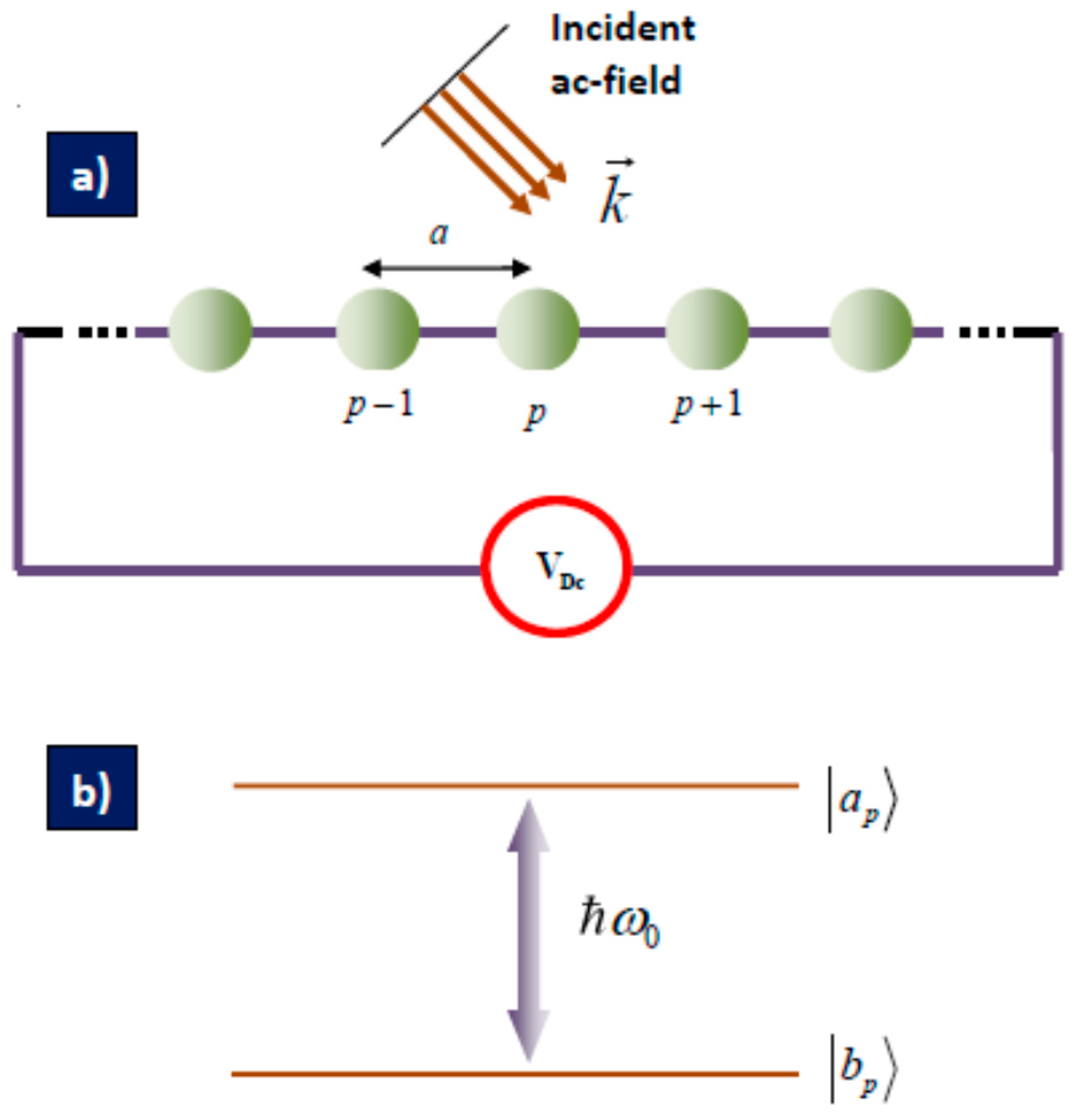
Figure 1.
(a) General illustration of the periodic two-level atomic chain used as a model, indicating Rabi–Bloch oscillations (RBO) in strong coupling regime. It is excited with obliquely incident ac field, and driven with dc voltage applied at the ends. The neighboring atoms are coupled via interatomic tunneling, with different values of penetration at the ground and excited states; (b) Ground and excited energy levels of single two-level atom separated by the transition energy .

Figure 2.
General illustration of the periodic chain used as a model, indicating RBO in ultrastrong coupling regime. (a) The single element of the chain. It corresponds to a highly doped quantum well (QW) inserted inside the capacitor of microcavity of THz frequency range [43]. It is resonantly coupled with a mode of microcavity. The frequency matching is reached via the choice of inductance value; (b) A highly doped QW inserted inside the capacitors of the chain of coupled microcavities. The dc voltage applied to the system at the ends of the chain. The THz oscillating voltage is applied through a nano-antenna; (c) The periodic potential induced by additional doping for transforming the homogeneous QW to the effective superlattice. The coupling is governed by the inter-barrier electron tunneling.
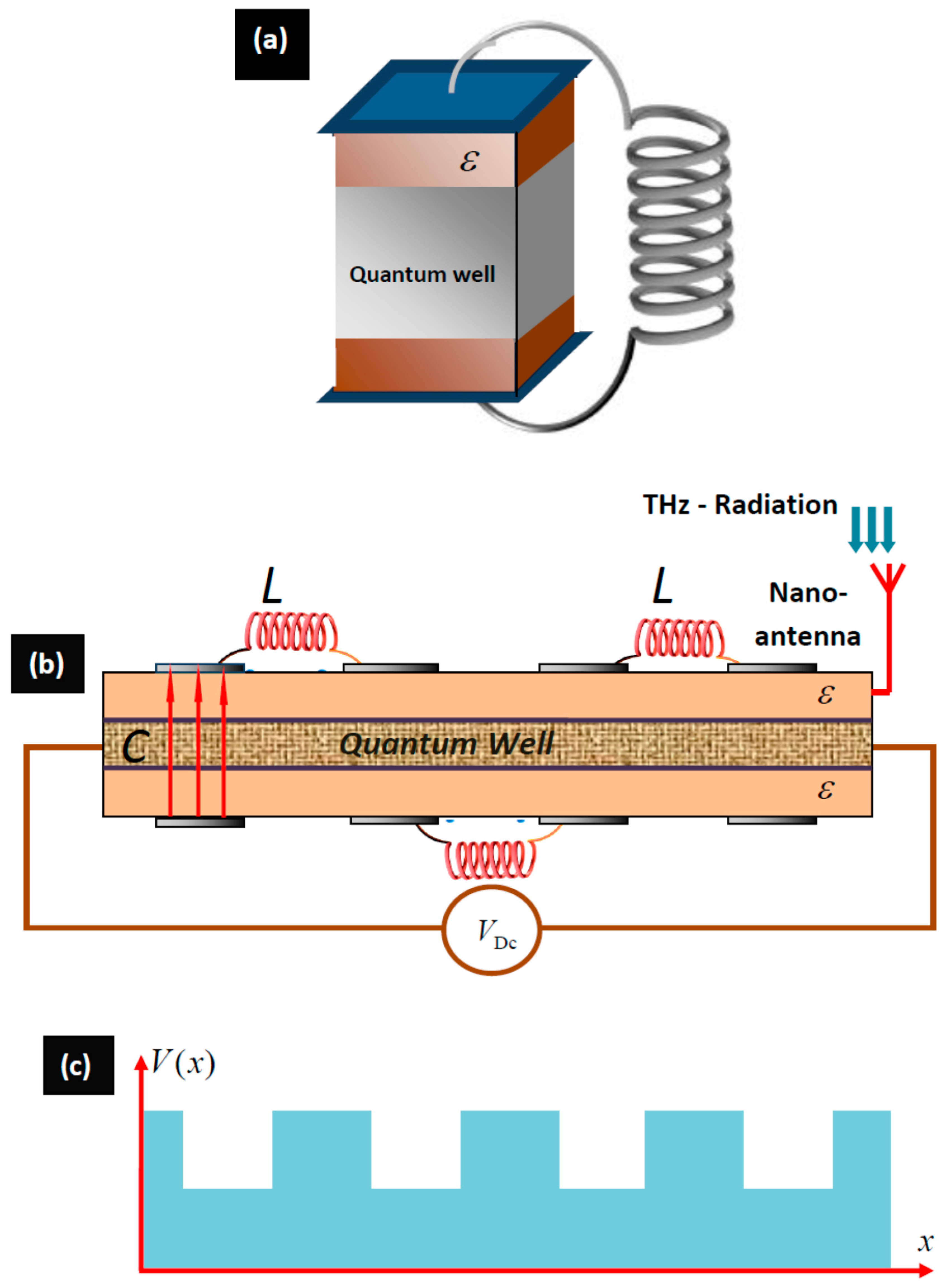
Figure 3.
Space–time distribution of the tunnel current density with Rabi-oscillations (RO) and Bloch-oscillations (BO) in the separated frequency ranges. Here, the quantum transition frequency is taken as the frequency unit, detuning is equal to zero , , , , , interatomic distance . The initial state of the chain is an excited single Gaussian wave packet , . Gaussian initial position and width are , , respectively. Number of atoms .

Figure 4.
Space-time distribution of the tunnel current density with RO and BO in the separated frequency ranges. . All other parameters are identical to Figure 3.
Figure 4.
Space-time distribution of the tunnel current density with RO and BO in the separated frequency ranges. . All other parameters are identical to Figure 3.
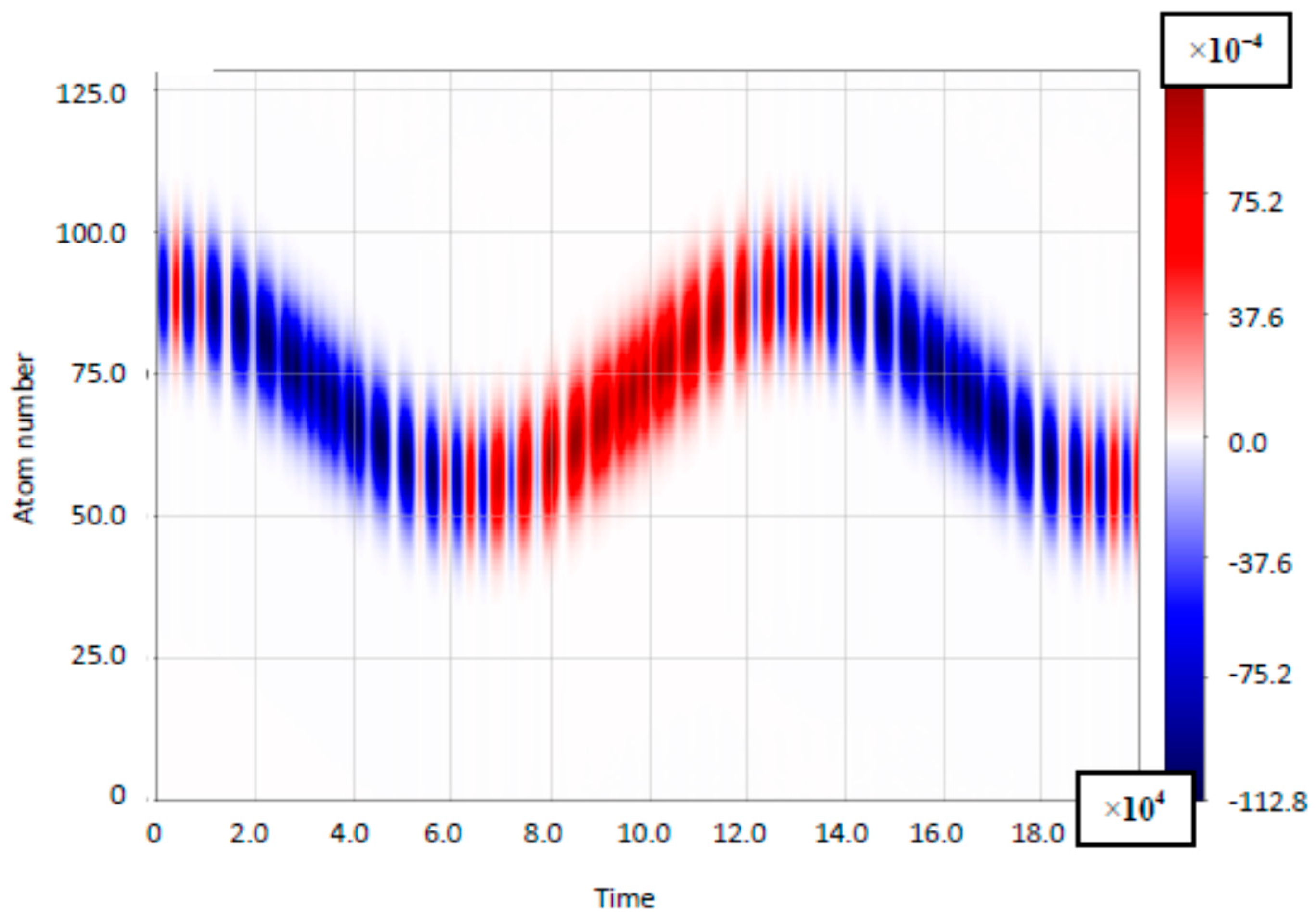
Figure 5.
Frequency spectrum of the tunneling current density with RO and BO in the separated frequency ranges at the atomic position with number . The quantum transition frequency, Rabi-frequency and Bloch-frequency are denoted by a red-colored dashed line, blue-colored dashed–dotted line and green-colored dotted line, respectively. The quantum transition frequency is taken as the unit. , . All other parameters are identical to Figure 3.

Figure 6.
Frequency spectrum of the density of the tunneling current with RO and BO in the separated frequency ranges. . All other parameters are identical to Figure 5.
Figure 6.
Frequency spectrum of the density of the tunneling current with RO and BO in the separated frequency ranges. . All other parameters are identical to Figure 5.
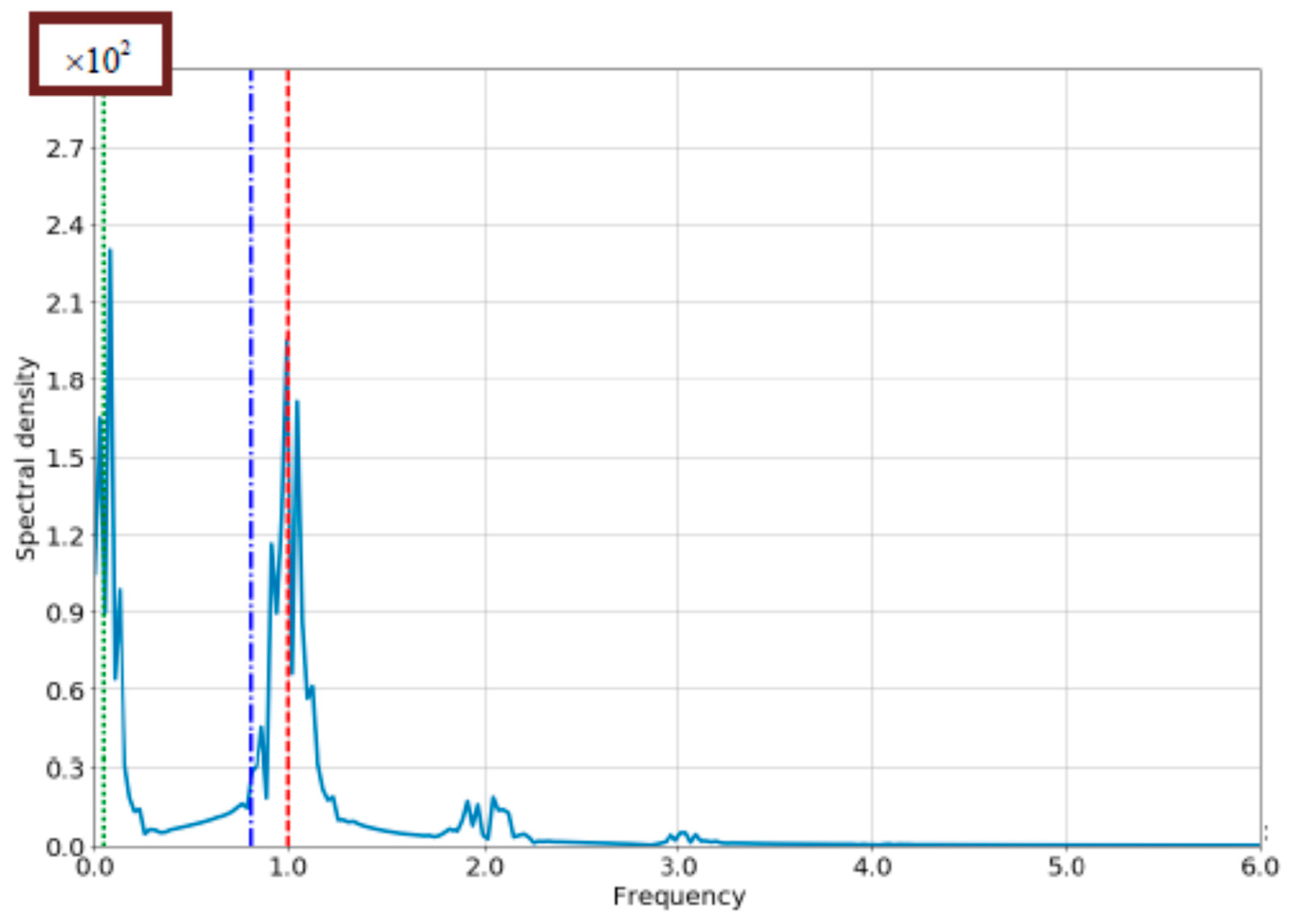
Figure 7.
Space–time distribution of the dipole moment density with RO and BO in the separated frequency ranges. All parameters are identical to Figure 3.
Figure 7.
Space–time distribution of the dipole moment density with RO and BO in the separated frequency ranges. All parameters are identical to Figure 3.
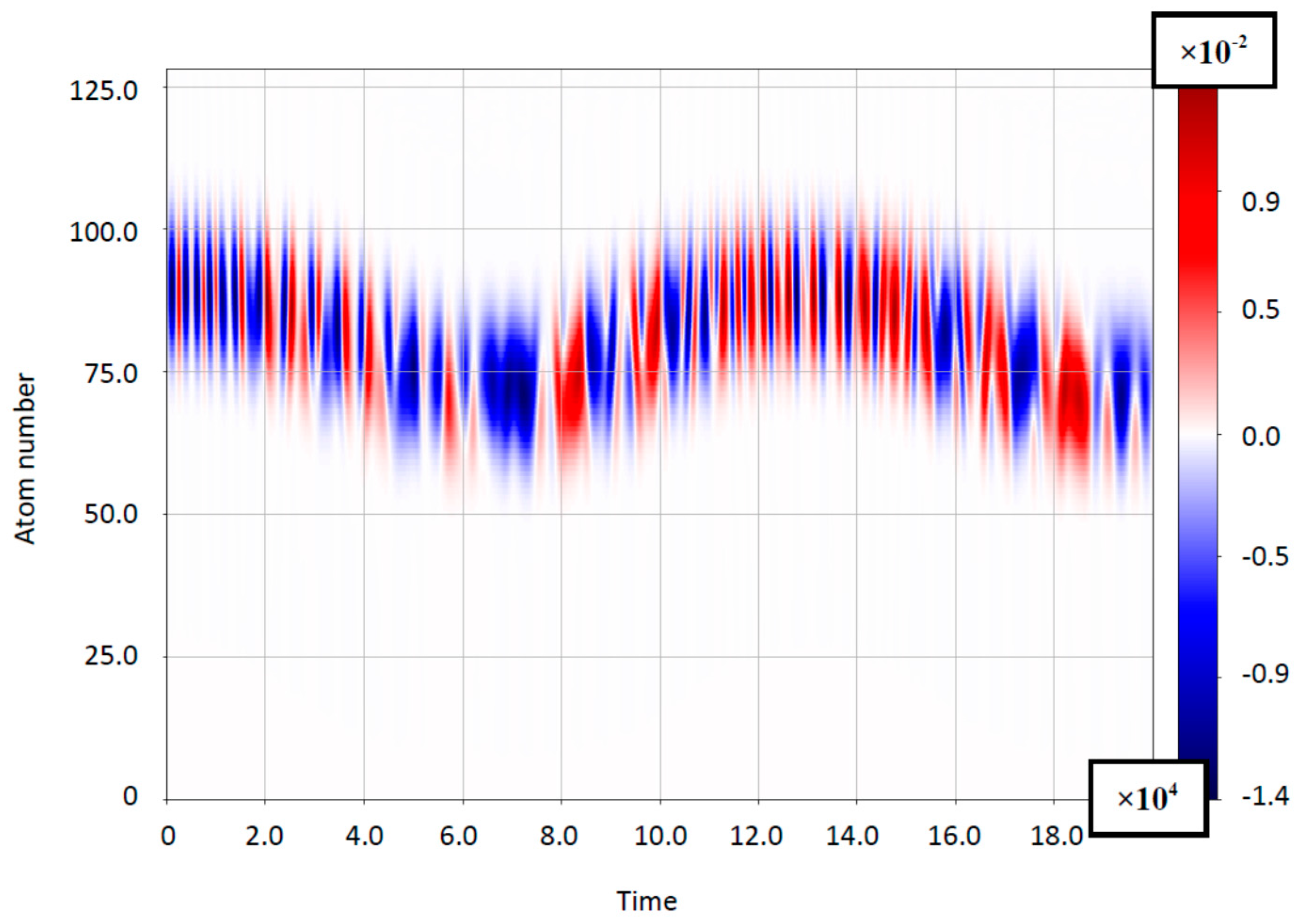
Figure 8.
Space–time distribution of the inversion density with RO and BO in the separated frequency ranges. All parameters are identical to Figure 3.
Figure 8.
Space–time distribution of the inversion density with RO and BO in the separated frequency ranges. All parameters are identical to Figure 3.

Figure 9.
Frequency spectrum of the dipole moment with RO and BO in the separated frequency ranges at the atom with position number . All parameters are identical to Figure 3.
Figure 9.
Frequency spectrum of the dipole moment with RO and BO in the separated frequency ranges at the atom with position number . All parameters are identical to Figure 3.
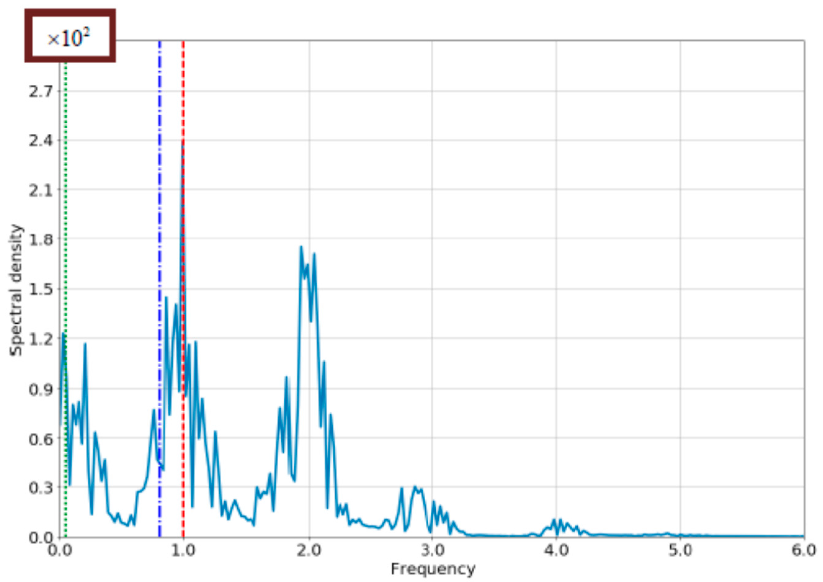
Figure 10.
Frequency spectrum of inversion density with RO and BO at the separated frequency ranges at the atomic position . All parameters are identical to Figure 3.
Figure 10.
Frequency spectrum of inversion density with RO and BO at the separated frequency ranges at the atomic position . All parameters are identical to Figure 3.

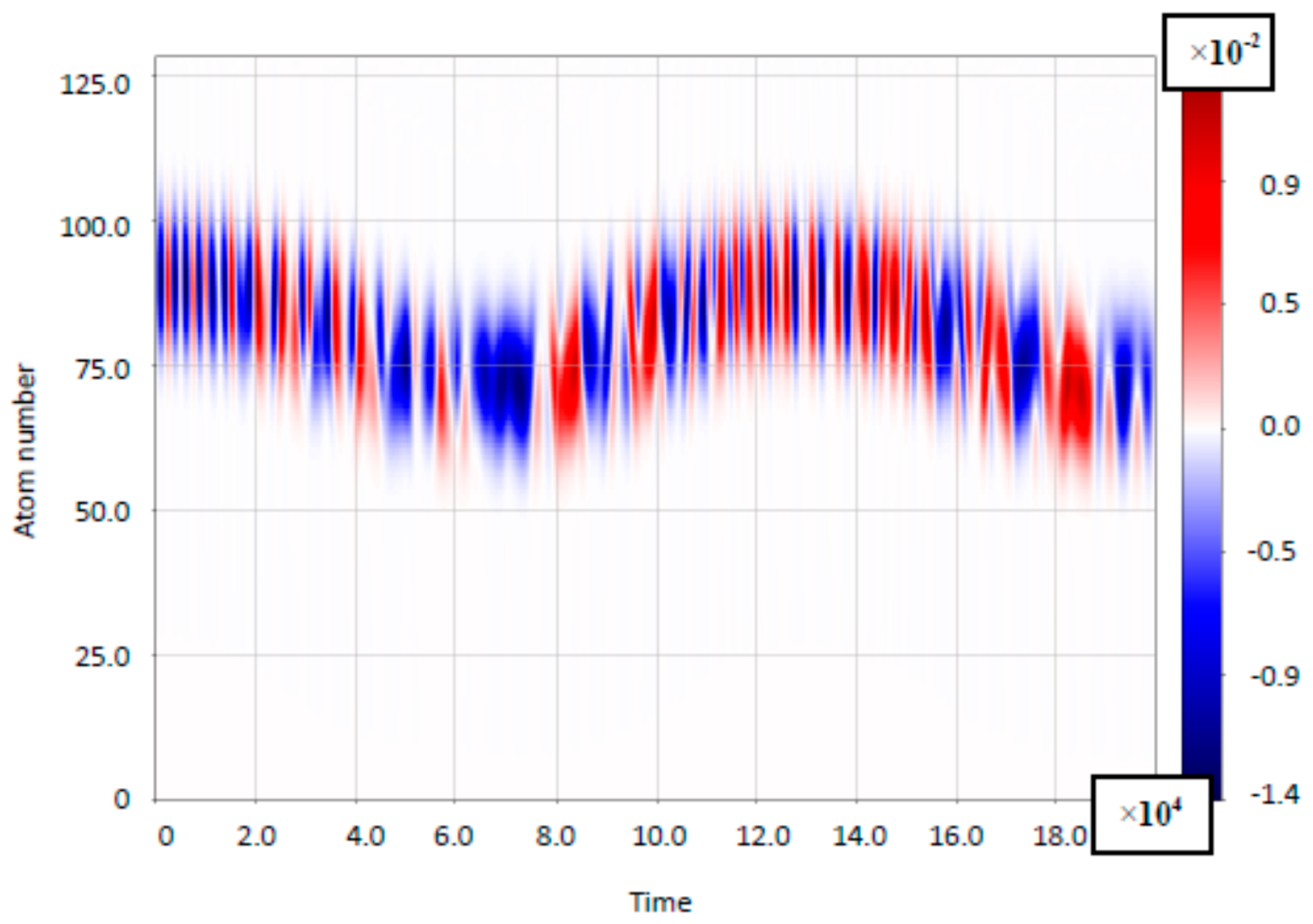
Figure 11.
The space–time distribution of the tunnel current density with RBO in the ultrastrong coupling regime. Here, the quantum transition frequency is taken as the frequency unit, zero detuning , , , , and interatomic distance . The initial state of the chain is an excited single Gaussian wave packet , . Gaussian initial position and width are , , respectively. Number of atoms .
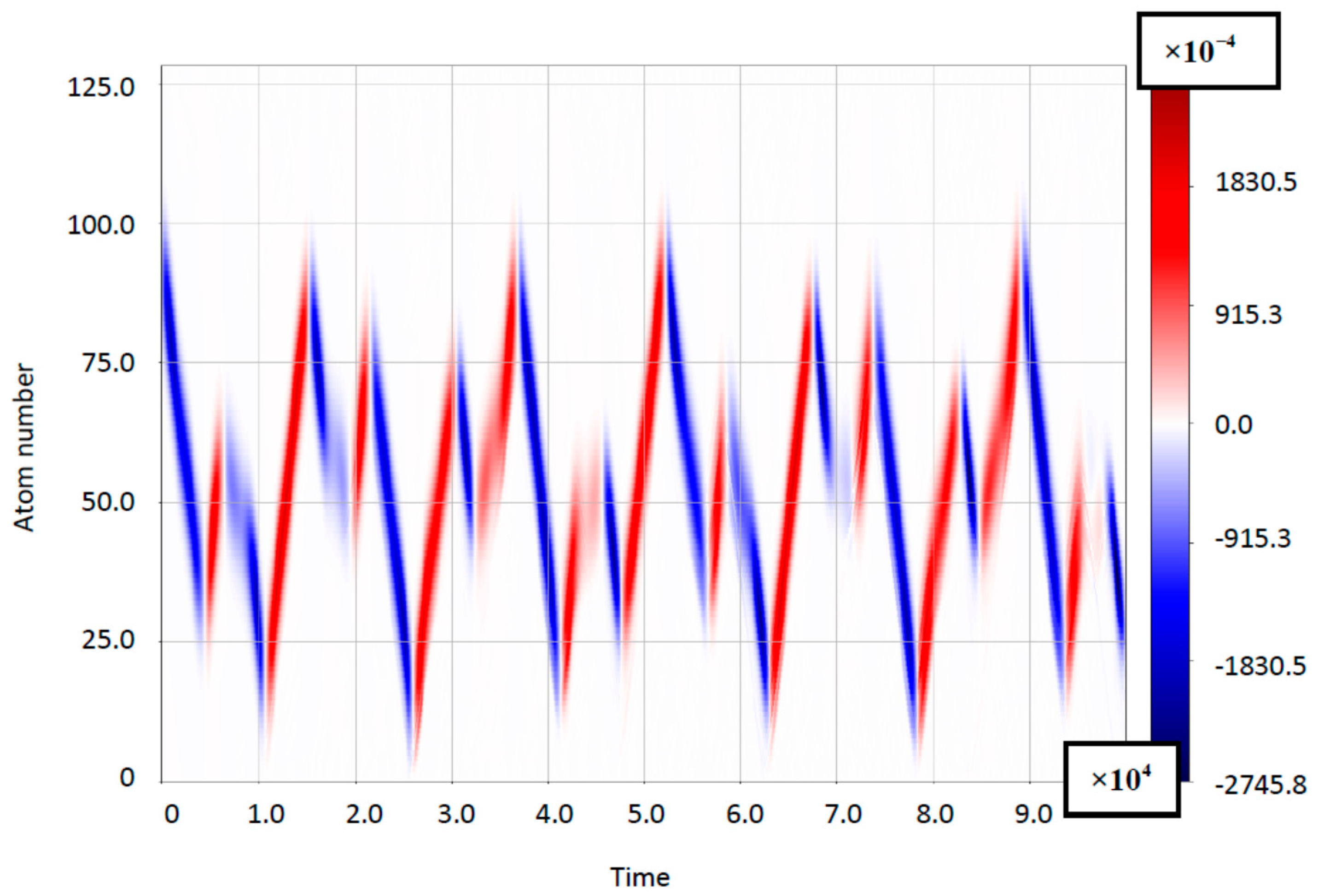
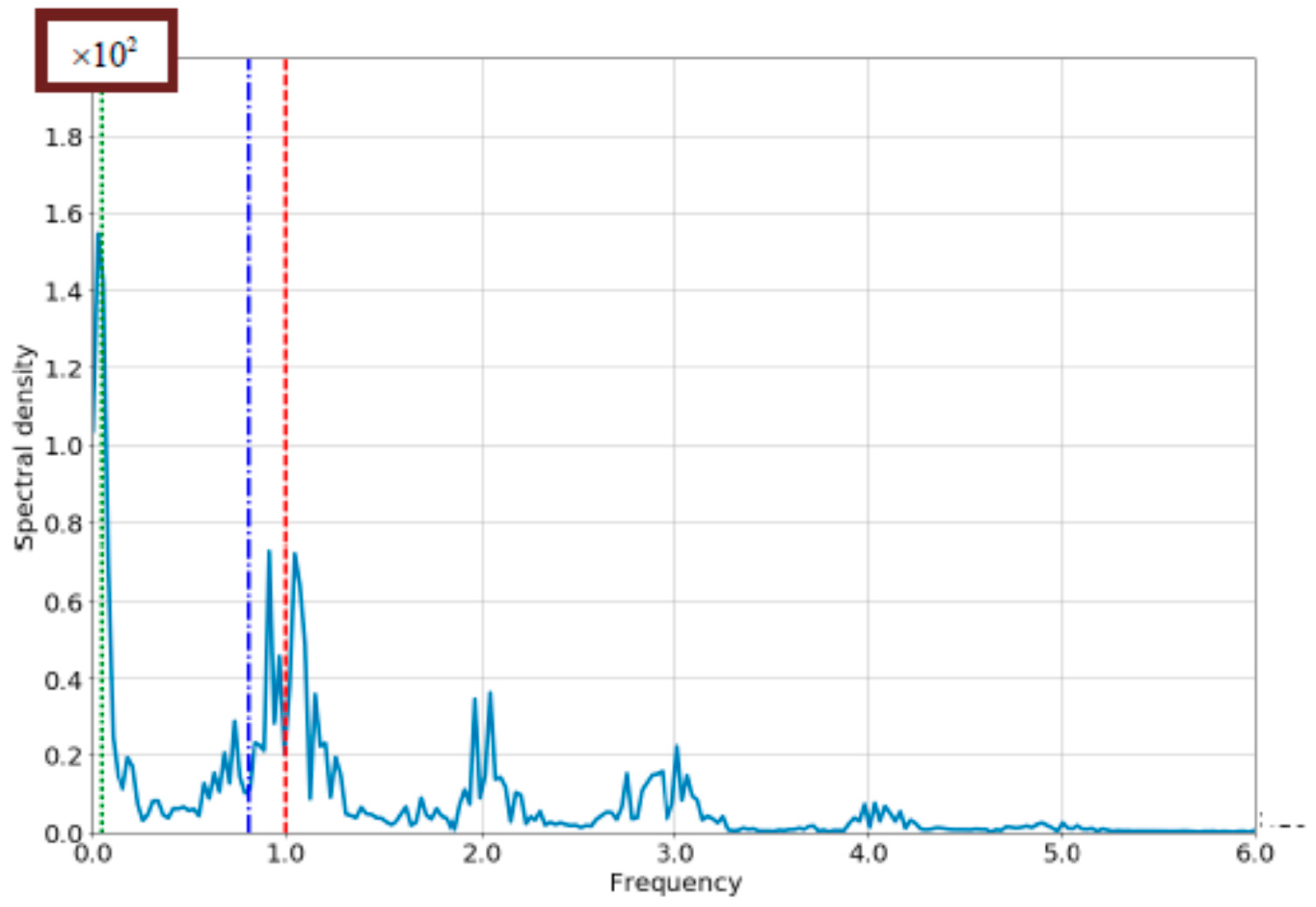
Figure 12.
The frequency spectrum of tunnel current density with RBO in ultrastrong coupling regime at the atomic position . All parameters are identical to Figure 11.
Figure 12.
The frequency spectrum of tunnel current density with RBO in ultrastrong coupling regime at the atomic position . All parameters are identical to Figure 11.
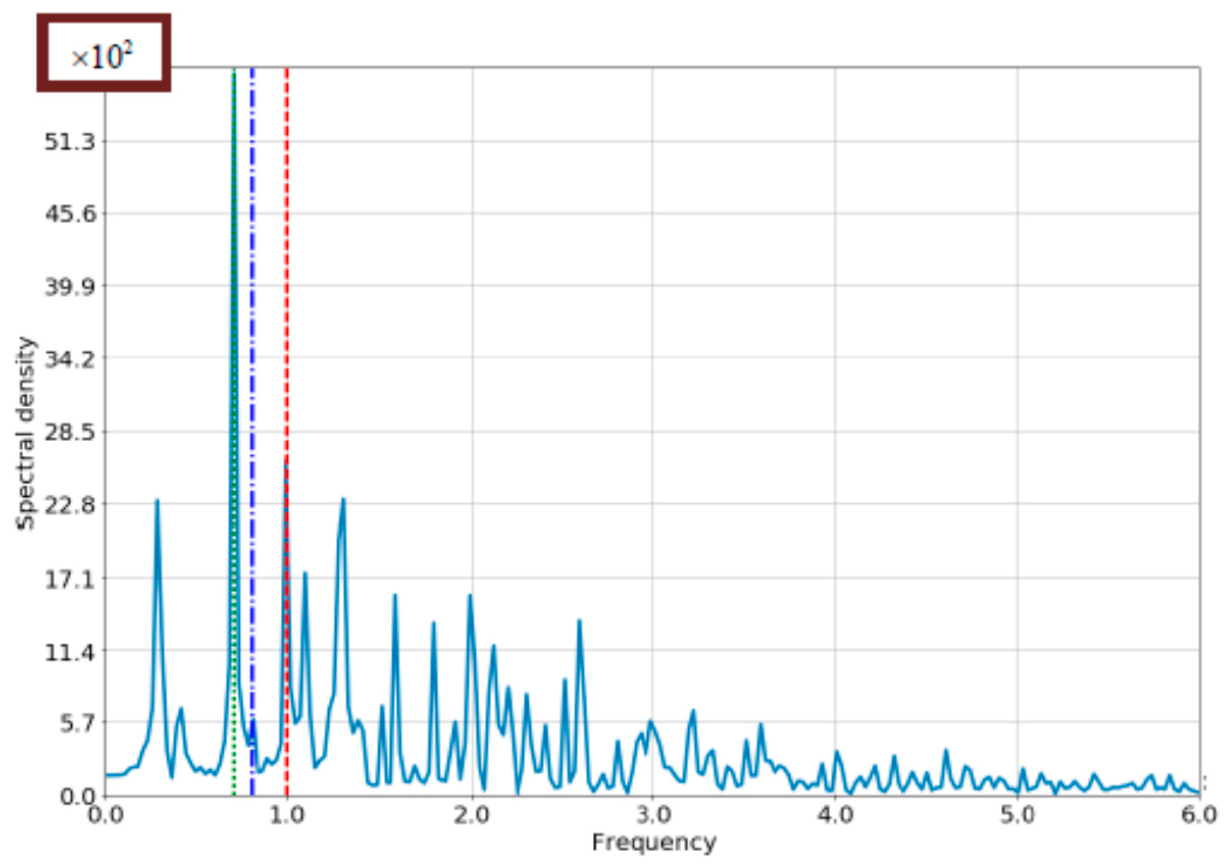
Figure 13.
The frequency spectrum of the tunnel current density with RBO in the ultrastrong coupling regime at the atomic position . , . All other parameters are identical to Figure 11.
Figure 13.
The frequency spectrum of the tunnel current density with RBO in the ultrastrong coupling regime at the atomic position . , . All other parameters are identical to Figure 11.
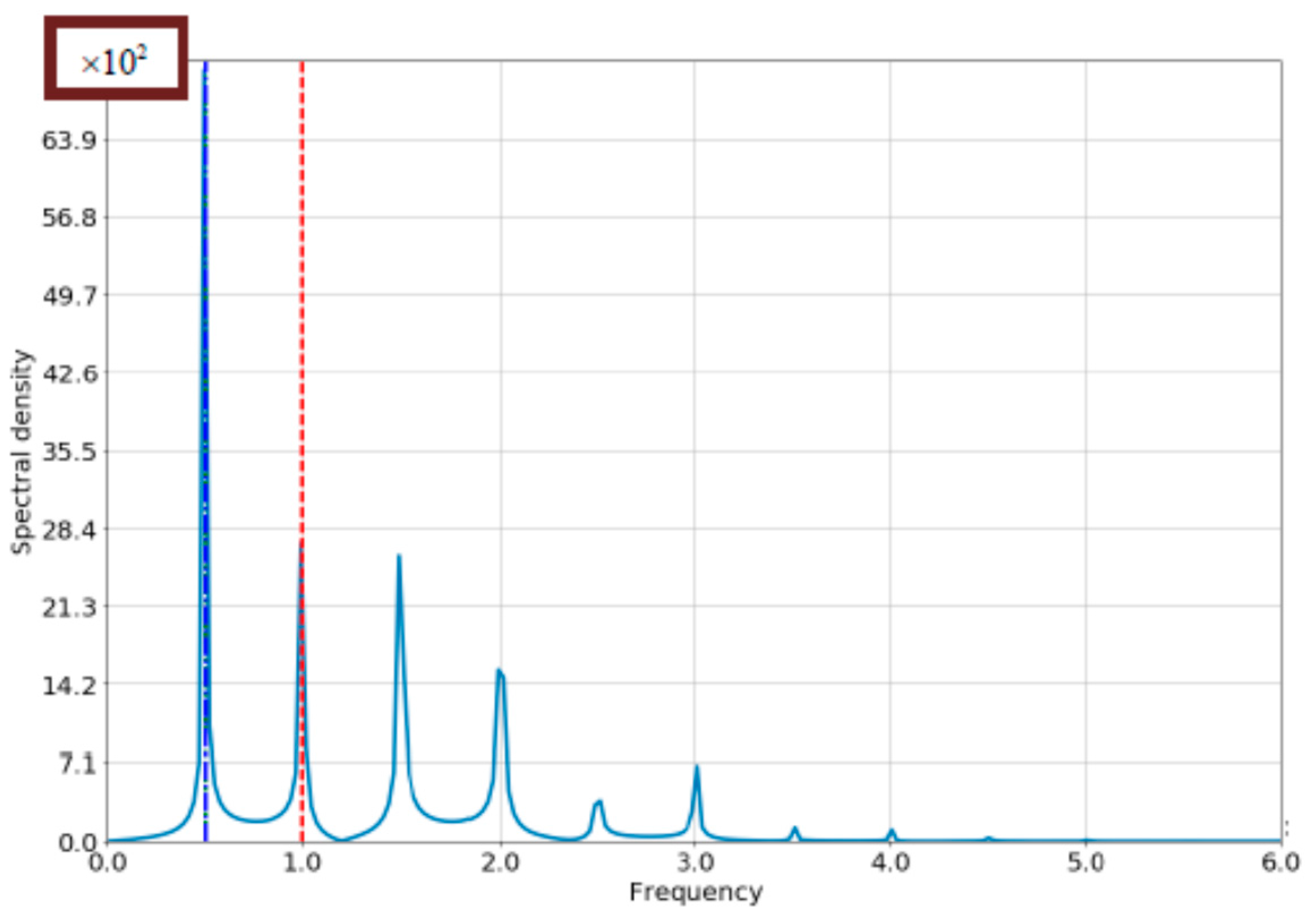
Figure 14.
The frequency spectrum of the dipole moment density with RBO in the ultrastrong coupling regime at the atomic position . , .
Figure 14.
The frequency spectrum of the dipole moment density with RBO in the ultrastrong coupling regime at the atomic position . , .

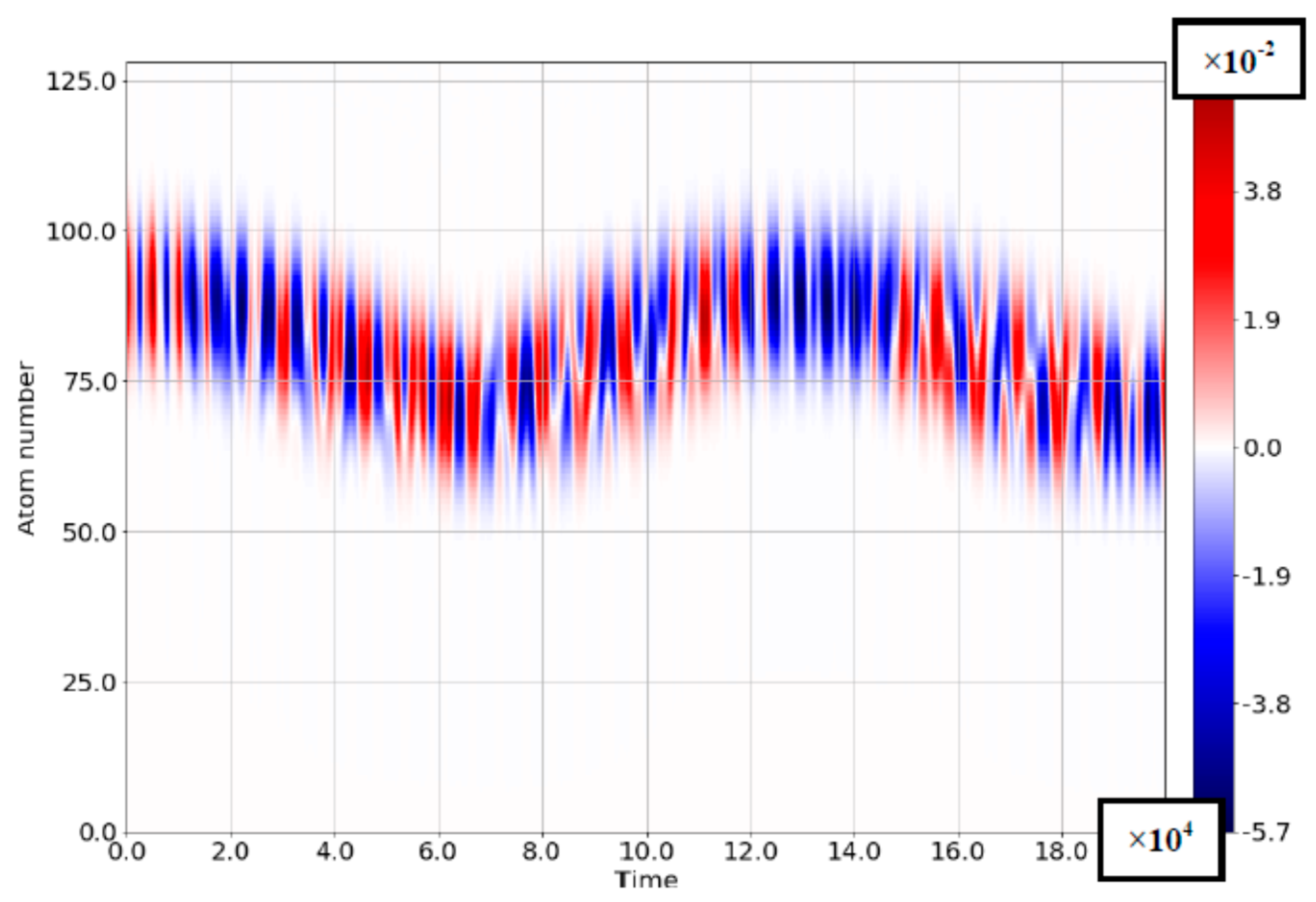
Figure 15.
The space–time distribution of tunneling current density with RBO in the ultrastrong coupling regime with dissipation. Insert: the individual energy spectrum of the single atom in the chain. The model assumes that two levels decay at a rate , due to spontaneous emission. Thus, the ground state is not really ground; it corresponds to the excited state at the lowest energy level. The dissipation property is characterized by a Q-factor, defined as . Realistic values for ultrastrong coupling cases are Q = 15–30 [43]. Here, the quantum transition frequency is taken as the frequency unit, detuning is zero , , , , interatomic distance , and Q = 15. The initial state of the chain is an excited single Gaussian wave packet . Gaussian initial position and width are , , respectively. Number of atoms .
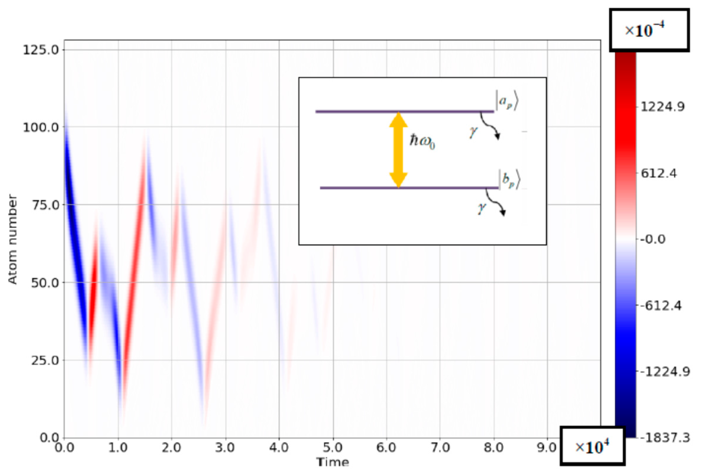
Figure 16.
The frequency spectrum of tunneling current density with RBO in the ultrastrong coupling regime with dissipation in the atomic position . All other parameters are identical to Figure 15.
Figure 16.
The frequency spectrum of tunneling current density with RBO in the ultrastrong coupling regime with dissipation in the atomic position . All other parameters are identical to Figure 15.
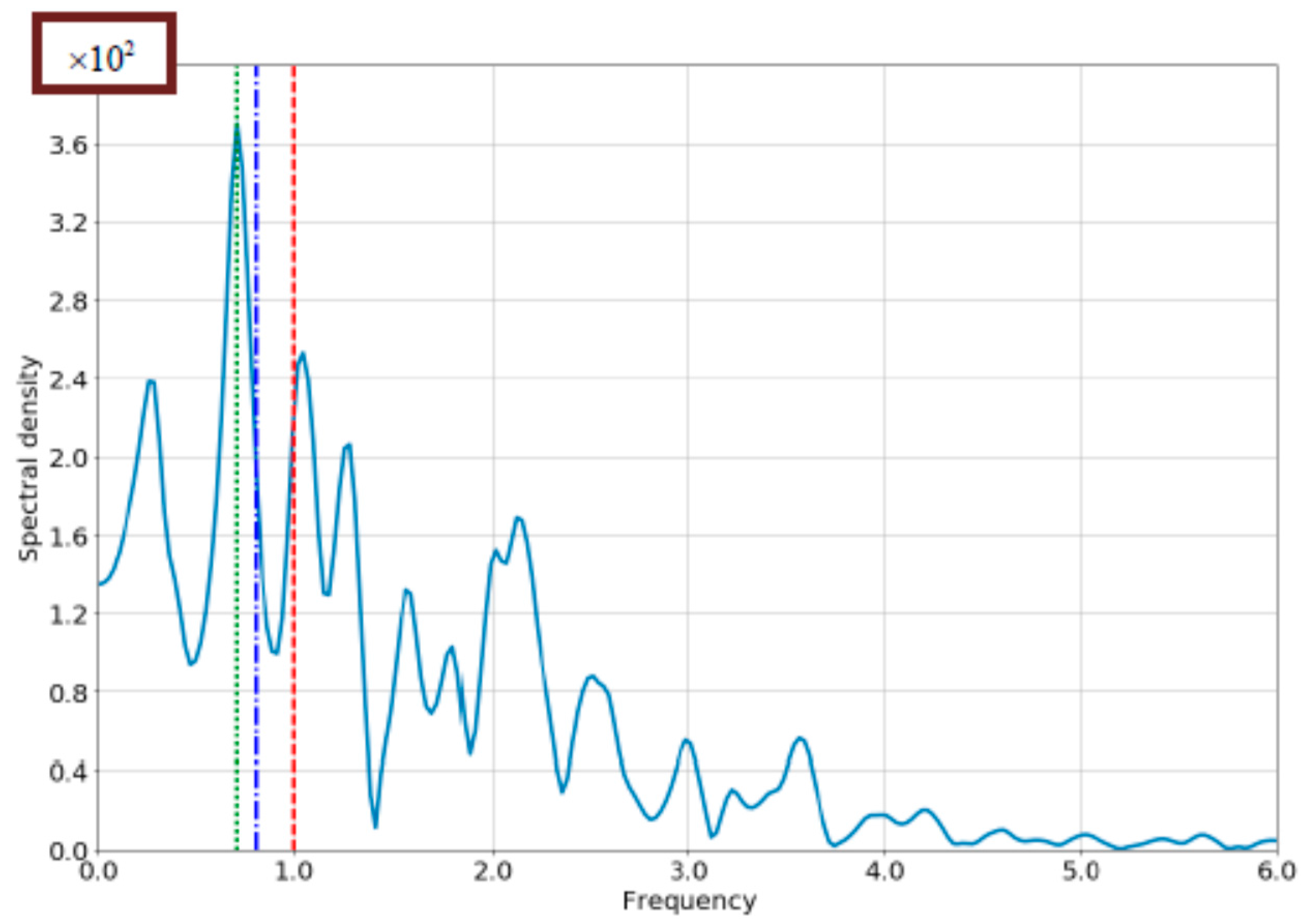
Figure 17.
The frequency spectrum of tunneling current density with RBO in the ultrastrong coupling regime with dissipation in the atomic position . , . All other parameters are identical to Figure 15.
Figure 17.
The frequency spectrum of tunneling current density with RBO in the ultrastrong coupling regime with dissipation in the atomic position . , . All other parameters are identical to Figure 15.

Figure 18.
General illustration of the periodic two-level atomic chain used as a model, indicating Stark effect in the ultrastrong coupling regime. The chain is placed obliquely between the armatures of plane capacitor with applied dc voltage. The dipole moments (blue arrowheads) are oriented orthogonally to the chain axis. Dc field (red arrowheads) are oriented angularly with respect to the chain axis. The choice of the angle allows for obtaining the arbitrary relative value between Rabi- and Bloch frequencies.

Figure 19.
Space–time distribution of inversion density with Stark effect. The initial state of the chain is an excited single Gaussian wave packet , . Gaussian initial position and width are , , respectively, , , number of atoms .
Figure 19.
Space–time distribution of inversion density with Stark effect. The initial state of the chain is an excited single Gaussian wave packet , . Gaussian initial position and width are , , respectively, , , number of atoms .
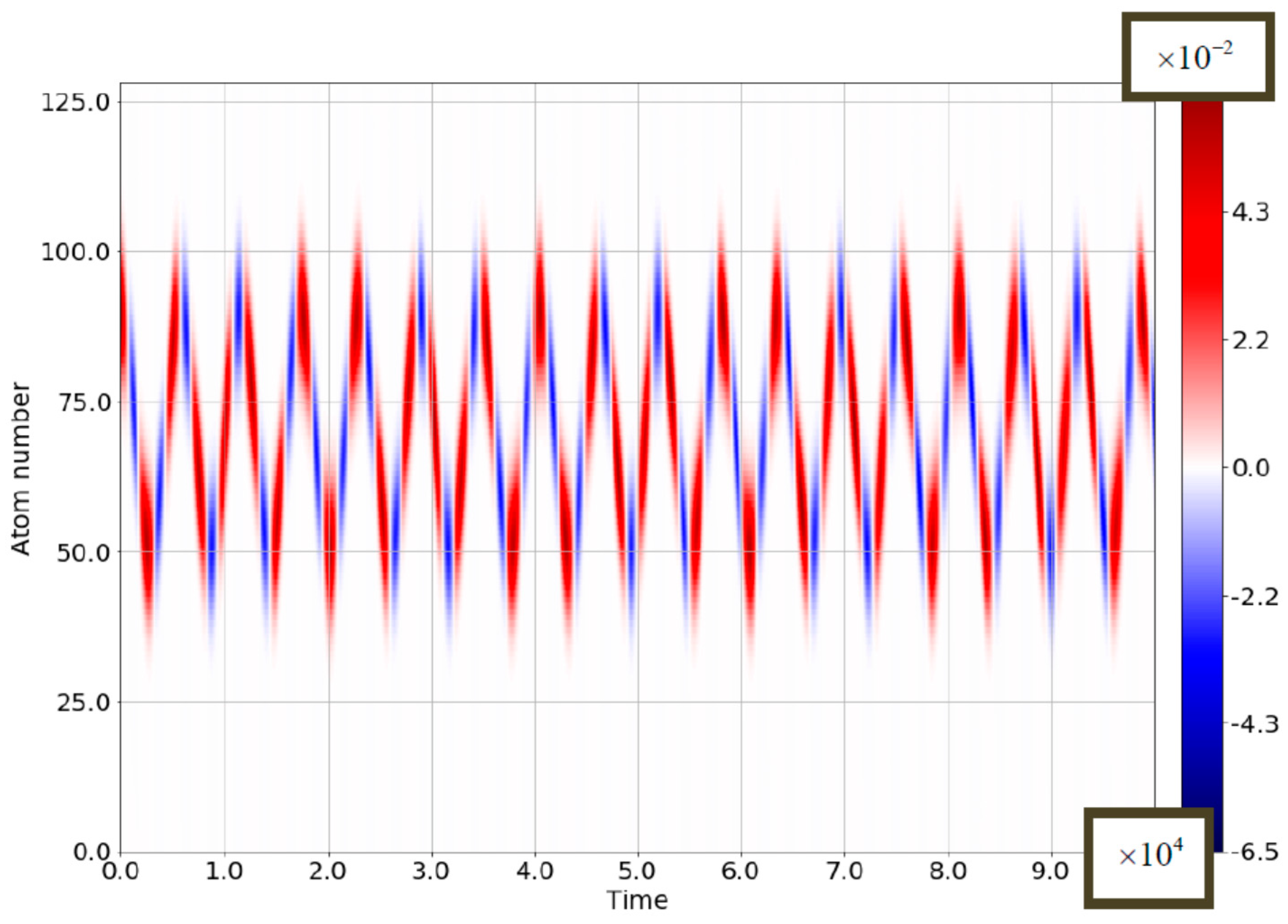
Figure 20.
Space–time distribution of tunneling current density with Stark effect. All parameters are identical to Figure 19.
Figure 20.
Space–time distribution of tunneling current density with Stark effect. All parameters are identical to Figure 19.

Figure 21.
The frequency spectrum of tunneling current density with Stark effect. All parameters are identical to Figure 15.
Figure 21.
The frequency spectrum of tunneling current density with Stark effect. All parameters are identical to Figure 15.

© 2017 by the authors. Licensee MDPI, Basel, Switzerland. This article is an open access article distributed under the terms and conditions of the Creative Commons Attribution (CC BY) license (http://creativecommons.org/licenses/by/4.0/).
Share and Cite
MDPI and ACS Style
Levie, I.; Slepyan, G. The New Concept of Nano-Device Spectroscopy Based on Rabi–Bloch Oscillations for THz-Frequency Range. Appl. Sci. 2017, 7, 721. https://doi.org/10.3390/app7070721
AMA Style
Levie I, Slepyan G. The New Concept of Nano-Device Spectroscopy Based on Rabi–Bloch Oscillations for THz-Frequency Range. Applied Sciences. 2017; 7(7):721. https://doi.org/10.3390/app7070721
Chicago/Turabian StyleLevie, Ilay, and Gregory Slepyan. 2017. "The New Concept of Nano-Device Spectroscopy Based on Rabi–Bloch Oscillations for THz-Frequency Range" Applied Sciences 7, no. 7: 721. https://doi.org/10.3390/app7070721
Note that from the first issue of 2016, this journal uses article numbers instead of page numbers. See further details here.