
Enhanced Adaptive Filtering Algorithm Based on Sliding Mode Control for Active Vibration Rejection of Smart Beam Structures


1
School of Mechanical Engineering, Yeungnam University, 280, (Dae-dong) Daehak-ro, Gyeongsan-si, Gyeongsangbuk-do 38541, Korea
2
Department of Mechatronics Engineering, Incheon National University, (Songdo-dong) 119 Academy-ro, Yeonsu-gu, Incheon 22012, Korea
*
Author to whom correspondence should be addressed.
Appl. Sci. 2017, 7(7), 750; https://doi.org/10.3390/app7070750
Submission received: 3 July 2017
/
Revised: 18 July 2017
/
Accepted: 19 July 2017
/
Published: 24 July 2017
(This article belongs to the Section Mechanical Engineering)
Abstract
:This article investigates vibration rejection for a continuous smart structure using piezoelectric bimorph patches. Such a structure has inherent nonlinearities, such as hysteresis and creep, and the whole system may experience unexpected disturbances, uncertainties, and noise from external sources. Thus, it is very important to design the active control scheme carefully with adaptive filtering systems to deal with these conditions. An advanced adaptive filtering algorithm was developed based on the conventional least mean squares (LMS) method and sliding mode control for the active vibration rejection system. The sliding mode controller is applied to the standard LMS algorithm to overcome problems with misadjustment and excess error in an optimal manner. A numerical analysis and laboratory experiment show that the technique can significantly attenuate the vibration of the smart structure at different levels and broadband frequency spectra. In addition, unidentified impedance is chosen to change the distribution of the mass, and the robustness and the adaptivity of the proposed approach are verified. The experimental results show that the method can isolate impulse-type vibrations of at least 2.8 dB, even with the adjusted mass arrangement.
1. Introduction
The primary structural components that experience external forces are usually modeled as continuous cantilevered beams in engineering structures such as vehicles, aircrafts, buildings, and bridges. Such structures commonly have dynamic behavior, which cannot be modeled perfectly and occur from unexpected external sources. These influences could induce undesirable vibrations, resulting in fatigue and likely severe failure. Smart structures with active control methods are one possible solution for isolating these detrimental vibrations, but the control system itself and mistuned control parameters can cause instabilities. Therefore, it is important to design control methods that are inherently insensitive to parameter changes to attenuate structural vibrations.
Lead zirconate titanate (PZT) patches have a number of real-world applications for active control for reducing noise, vibration, and harshness (NVH). Some automotive parts have thin walls and can transmit unexpected noise and vibration from many sources. Thus, there have been many efforts to apply PZT patches to automotive parts such as the body panels [1], muffler system [2], and powertrain oil pan [3]. PZT patches are also used for mechanical and aerodynamic NVH reduction applications, such as aircraft fin-tips [4], rotorcraft blades [5], and aeroelastic flutter [6]. PZT patches are also used in active fault detections and energy harvesting devices.
Piezoelectric shunt circuits can control vibrations from the actuator arms of hard disk drives [7], and they can be used for detecting or fixing cracked beams [8,9]. A hybrid-type switching control method has been used in order to isolate unwanted vibration as well as to improve the energy efficiency [10]. Active vibration isolation techniques have been implemented with piezoelectric actuators and sensors for the functionally graded material beams [11]. A smart structure with shunted piezoelectric patches was constructed, and topology optimization was performed for maximizing the electromechanical coupling factor in terms of the damping efficiency, piezo patch geometries, and patch locations [12]. A visualization technique was proposed to identify and reduce the vibrational energy of a 2D plate using a constrained damping layer [13].
To achieve satisfactory vibration attenuation, the structures and vibrational responses should be analyzed. An analytical solution was introduced for a piezoelectric bimorph cantilever beam with suitable boundary conditions [14]. The Airy stress function can also be used to study other different piezoelectric cantilevers, including multilayer piezoelectric cantilevers under different loads. The active vibration control of parametrically excited systems with resonance was examined to avoid the parametric instability, and an active control system was introduced, which includes a beam subjected to an axial harmonic load [15]. An enhanced method was proposed to stabilize the system via velocity feedback and pole placement by relocating the transition curves. Finally, generally layered smart beams were observed with a one-dimensional finite element method [16]. This state space model is based on first-order shear deformation beam theory with Hermite shape functions and the effect of external electric loads.
Appropriate control algorithms must be designed for individual systems to achieve desirable performance. Piezoelectric shunt circuits have been applied extensively for the semi-active control of vibrating structures, but a single piezoelectric shunt circuit can deal with only one vibration mode at a time [17]. Many methods have been explored to manage more than one mode, such as multiple piezoelectric shunt circuits [18], synchronized switch voltage damping [19], and periodic piezoelectric shunts [20]. However, these techniques are still passive methods, for which adjustment is needed in advance. Thus, a number of active control schemes have been examined. These schemes include positive position feedback [21,22], acceleration feedback [23,24], full-state feedback [25], dynamic hysteresis compensators [26], pole placement control [27], and a hybrid of variable structure control and Lyapunov-based control [28]. Decoupled models were proposed to manage many degrees of freedom (DOF), and a backstepping method was introduced to design a robust controller with sliding mode and adaptive strategies [29]. To avoid the high computational burden of full-order controllers, a direct minimization method was introduced to design reduced-order H-infinity controllers and genetic algorithms [30].
The conventional approaches for active vibration control are often too complicated and thus difficult to implement. Furthermore, the control targets have to be determined, which limits the tracking, convergence, and stability performance. If a correct mathematical model of flexible structures can be derived, the structures can be regulated actively to isolate the structural vibration. However, several control schemes show performance degradation when the model is not precise enough and the structural dynamics varies with time due to structural modifications. To solve these issues, a simple and robust control algorithm should be developed without any correlation to the original structural dynamics and with low computational burden.
This study uses an enhanced active vibration control method attenuate the vibration of a nonlinear elastic smart structure. A new control scheme called as the sliding mode least mean squares (SM-LMS) algorithm is proposed and validated both numerically and experimentally [31]. The control algorithm combines the optimal control characteristics of the least mean squares algorithm with the robustness of sliding mode control (SMC). It has been shown that SM-LMS can be successfully used for the displacement control of piezoelectric actuators [32]. However, no study has applied SM-LMS to the active vibration control of flexible structures. To validate the scheme, the controller was implemented on a smart structure constructed with an aluminum beam with two PZT actuators attached to form a bimorph structure and one PZT sensor. For the actual tests, we would not know the exact model of the system due to unknown changes in the operating environment, and the plant may vary over time. This changes the control parameters needed to achieve the best tracking performance. Thus, experiments of two different cases were prepared: (1) control for a baseline structure; and (2) control for a structure with additional dynamics that cannot be predicted. Additional impedance is added to the baseline structure to simulate a sudden change in the plant. The scope is limited to a single-input single-output system, and the first four peaks of the disturbance plant (the natural modes) are considered. Specific objectives of this research are described below.
- (1)
- Introduce the characteristics of the novel nonlinear control methodology (sliding mode least mean squares) and examine the performance on active vibration control through numerical simulations.
- (2)
- Identify the dynamic model of the active beam in the frequency domain with an impact hammer test. Estimate parameters of the linear beam model through a frequency domain identification method.
- (3)
- Conduct numerical validations with a conventional approach for attenuating vibration level of the structure under impulsive excitations and observe limitations.
- (4)
- Conduct experimental validations and examine the performance of the controller for the baseline structure and the modified structures in order to show the robustness of the new control technique.
2. Adaptive Filtering Systems for Active Control
Conventionally, digital filters have been applied for modeling dynamic responses to any type of given inputs in engineering structures and acoustic platforms. They apply numerical processes in the discrete time domain for a certain signal to obtain a desired signal shape, and they are broadly used in electronics, computer science, and mechanical engineering. The finite impulse response (FIR) filter is extensively used to represent system responses because of its inherent simplicity, stability, and ease of implementation. In addition, digital filters notably applicable in adaptive structural design and control. Adaptive digital signal processing is applied to update digital filter coefficients automatically in order to create a desired signal from a reference signal and error based on recursive algorithms. Digital filters are thus commonly used in active noise and vibration isolation, system identification, and inverse modeling. An adaptive digital filtering system was designed for active control of the unwanted vibration of continuous structures with a new adaptive filtering algorithm.
2.1. Least Mean Squares Method
The least mean squares (LMS) algorithm is the most widely used feedforward control algorithm for adaptive digital filtering systems, since it is relatively simple and easy to implement. The stochastic gradient of the squared error signal is the core of this algorithm [33], and it iteratively regulates the coefficients of transversal filters. These filters use the following two values for the updating formulation: (1) a reference input containing frequency components to be dealt with; and (2) the measured error value at the current instant, which is the difference between the filter output and the disturbance (desired value) to be tracked. The algorithm adjusts the adaptive digital filter to determine a filter output that is as close as possible to the disturbance value . A formulation of the LMS algorithm for updating these coefficients can be derived by minimizing the mean squared error with a pre-defined cost function.
The most attractive feature of the LMS method is that it does not require average correlation functions from gradient estimates and matrix inversions [34]. It starts from the steepest descent method, and the output of the FIR filter is calculated by multiplying a reference vector by a vector of filter coefficients or weights . In Equation (1), is the reference input signal at time index , and is the jth filter coefficient at time index . The desired signal is the output of the disturbance plant to be tracked and reduced, and the error is the deviation between the filter output and the desired signal .
A cost function is chosen to minimize the error. The mean squared error is typically selected as a cost function since it is a quadratic function and thus guarantees a unique minimum, which is a very important advantage for the digital filtering system.
The cost function is expanded by substituting Equations (1) and (2) into Equation (3):
is a cross correlation vector between the reference input and the desired signal, and is the autocorrelation matrix of the reference signal. The steepest descent concept is used to develop an algorithm that adjusts the vector of filter weights . The reason why this method is applied here is that it is very straightforward and has been validated in many applications.
Next, Equation (7) is partially differentiated with respect to , and then the gradient of the cost function can be derived:
From Equations (7) and (8), the steepest descent algorithm is obtained:
where is a parameter that regulates the convergence speed and the stability of the adaptation procedure. Figure 1 shows a block diagram of a typical adaptive digital filtering system.
The gradient of the cost function is calculated in every iteration with an average of squared errors at recent sampling times. However, it is usually impossible to predict the cross correlation vector and the correlation matrix at every sample time. Thus, to simplify the updating equation for the filter coefficients, the LMS algorithm uses instant estimations for , , and the cost function [35]. Therefore, is chosen as an estimate of , and the correlation matrix and cross correlation vector are assumed to be:
Next, the estimation of the gradient of the cost function is obtained from Equations (8) and (10)–(12):
Finally, substituting Equation (13) into Equation (7), the final form of the LMS algorithm is derived.
Notably, the filter coefficients cannot trace the actual steepest descent surface because the changes of the weights are based on estimated or simplified gradients, which produce noisy tracking.
2.2. Filtered-X Least Mean Squares Method
In most practical applications, there are usually effects from secondary path dynamics due to AD/DA converters, filters, actuators, sensors, amplifiers, and circuit noise, among others. However, we assume that the whole control system includes no such dynamics and that the algorithm will not behave properly with such effects. The most common types of secondary path dynamics are phase shifts or time delays. The whole control structure become unstable or converges to an inappropriate solution under these effects, which changes the filter output and the signal subtracted from the desired signal .
The filtered-X LMS (FX-LMS) algorithm is a modified version of the traditional LMS algorithm that manages the secondary path dynamics, which are identified in advance [36]. This algorithm requires a filtered reference signal with a numerical model of the secondary path dynamics . The signal is applied in the original LMS algorithm to obtain the adaptive filter output . FX-LMS is more stable than the LMS method when the secondary path dynamics cannot be disregarded. Figure 2 shows a schematic of the FX-LMS algorithm.
The formulation for the FX-LMS algorithm is almost the same as that of the LMS method except that the filtered reference input is used in the updating equation of the filter weights:
The most important property of the filter is that its impulse response contains the same amount of time lag as the secondary path dynamics . However, a significant defect of FX-LMS is that an offline system identification procedure is essential to obtain beforehand. Although online system identification might be possible, it makes the overall controller complex and difficult to implement.
2.3. Limitations
Many studies have modified the LMS algorithm to address defects such as misadjustment and excessive error with respect to the reference inputs. Hybrid structures were proposed by combining the LMS method with feedback control [37,38]. The vibration isolation was improved at main frequencies and the speed of the convergence was increased, but the error over a broadband frequency range could not be managed. An alternative feedback structure was suggested with internal model control. This method achieves a better transient response and faster convergence, but an incorrect secondary path model seems to degrade the total control performance [39]. An LMS algorithm with adaptive step size was investigated to increase the convergence rate [40,41]. Similarly, a variable-step LMS scheme was applied along with a creep model to accomplish rapid convergence and stability and to identify the hysteresis parameters [42].
A variable convergence coefficient corresponding with an input signal can improve the performance, but it may result in noisy step sizes with unwanted disturbances and thus influence the mitigation at other frequencies [43]. Another LMS scheme prevents instability with impulsive noise, and the reference is pre-defined to assure stability and convergence, particularly when the magnitude of the signal is larger than a certain threshold [44]. An anti-saturation LMS algorithm was introduced to overcome the controller output with large disturbance, which showed improved performance. A different cost function is needed to obtain an enhanced recursive formulation [45].
An extra filter has been used to suppress disturbances in the primary path resulting from uncorrelated noise in the secondary path. This method accomplishes faster convergence, but additional filters increase the complexity and noise in the control system [46]. A new LMS algorithm with phase compensation was introduced to deal with signals that include DC components. The traditional LMS may not be effective for such signals, and when a high pass filter is used to eliminate the DC components, it can produce a phase variation [47].
3. Enhanced LMS Algorithm
3.1. Sliding Mode Control
SMC is one of the most popular nonlinear control methodologies in use today. The strength of this controller is that it is robust, insensitive to plant dynamics, and able to decouple higher-order systems, regardless of their nonlinearity and uncertainty [48]. Once a sliding surface is defined, the state trajectory moves between both sides of the surface by high frequency switching control with discontinuous inputs, and it eventually arrives on the pre-defined sliding surface. The motion of a system is not associated with its original dynamics, and it depends on only the sliding mode equation. The main advantage of SMC lies in its robustness and insensitivity to noise, since the system prescribes the dynamics associated with desirable performance characteristics and the system response is insensitive to disturbances or uncertainties in the system parameters [49].
The SMC design procedure includes the following two parts: (1) a discontinuity surface called the sliding surface is chosen to have dynamics related to desirable performance properties; and (2) a high-frequency switching control input is designed to drive the initial system states to the sliding surface. Because the discontinuous input leads the system states towards the sliding surface, the states eventually reach the surface and move along it, and this condition is referred to as “sliding mode.” The sliding surface is defined for linear systems:
where is a state vector, and is a row vector that decides the dynamics of the sliding mode. The discontinuous inputs and are then chosen to fulfill the requirements for the existence and the reachability of the sliding mode. A common model of the control input for linear system is:
where is a positive gain that is fairly large to insure so that the state trajectory will reach the sliding surface.
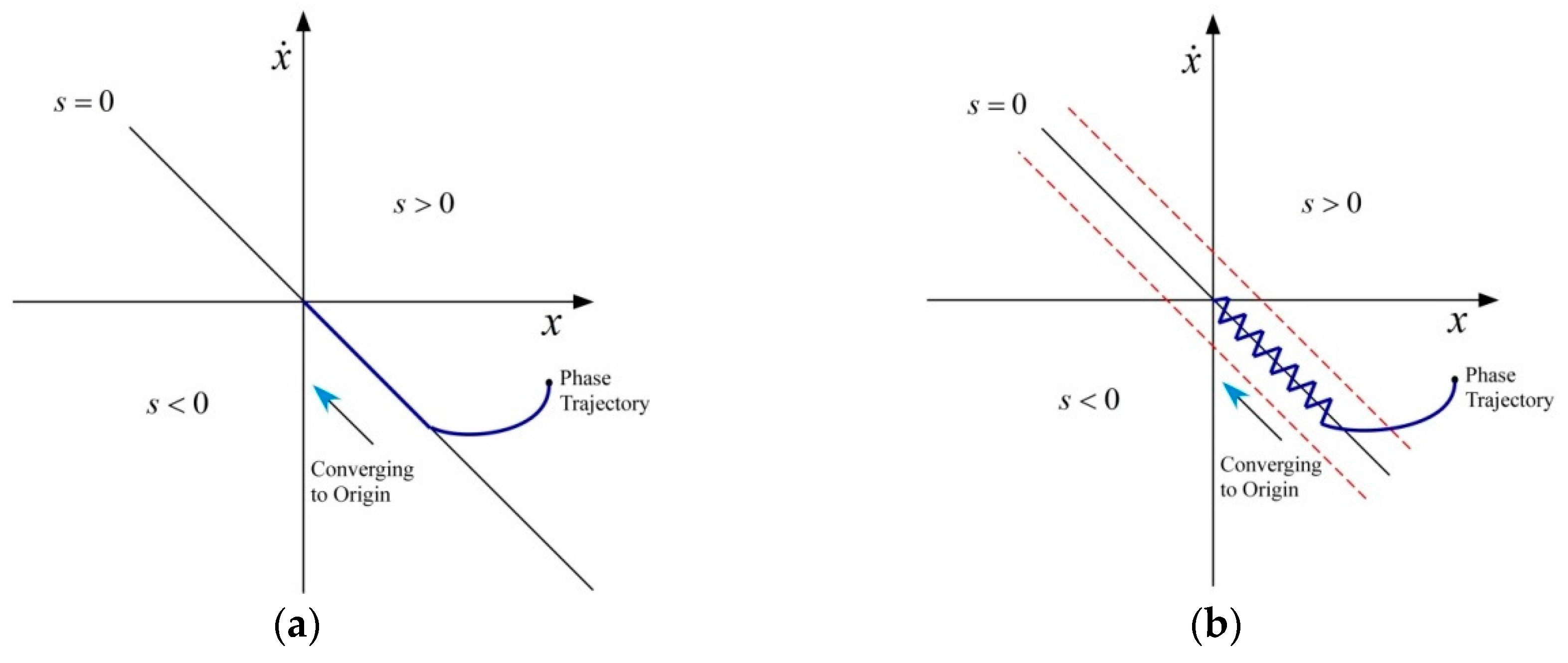
Figure 3 shows conceptual figures of an ideal sliding mode and a real sliding mode. The system trajectory in the state space arrives at the sliding surface defined by and slides towards the origin along the surface. To accomplish ideal sliding mode control, discontinuous control inputs should be able to switch at a fairly high frequency (theoretically infinite), as shown in the figure. However, most mechanical actuators cannot realistically replicate this condition, which results in chattering problems that could possibly make the overall system unstable when combined with unmodeled dynamics.
The SMC should also be considered in the discrete time domain since controllers are usually implemented on modern digital computers. For traditional discrete time sliding mode control (DSMC), the sliding mode is forced in the very next sampling moment [50], the point of which may cause controller saturation. The control system will then not work as expected and can even destabilize the target structure. Therefore, there is a need for a novel control technique that can solve these issues.
3.2. Sliding Mode LMS (SM-LMS)
A different structure of the adaptive filtering system is introduced using SMC for active vibration isolation. This new system prevents misadjustment from improper initial states and excessive error problems with respect to the amplitude of the desired values for the sake of the SMC. The sliding mode control is improved by the LMS in terms of smooth convergence and stability. With these properties, it is expected that the technique will enable multi-spectral control of disturbances to manage noise signals and a number of frequency elements simultaneously with optimized tracking schemes.
The SMC technique is combined with the LMS to track or control due to its intrinsic benefits of insensitivity to the plant dynamics, robustness, and ability to decouple systems with high dimension [49]. The proposed SM-LMS technique is illustrated in Figure 4.
in Figure 2 is defined as follows:
where indicates the jth filter coefficient at sampling index . is defined with the assumption that can be disregarded:
Next, the sliding mode in the error state plane is designated as follows. Here, α determines the slope of the sliding surface.
Using a similar procedure to the derivation of the LMS algorithm, the cost function for the SM-LMS is now defined as Equation (21), where means the expected value. Note that the cost function is applied in the LMS algorithm.
A unique minimum value is guaranteed since is a quadratic function. By expanding using Equations (4) and (20), the following results can be obtained:
The vector indicates the expected cross correlation between the reference and unwanted signals, and the matrix is the expected autocorrelation of the reference:
The next step is using the steepest descent scheme to obtain an algorithm for regulating the weights .
Equation (21) is partially differentiated with respect to in order to derive the gradient of the cost function :
For this control algorithm, the gradient along with and , have to be determined in every time instant , as mentioned in the previous section. This is a clumsy process, and to simplify the calculating operations, instantaneous estimates of , , and should be obtained at a specific sampling instant in the LMS algorithm [34]. Thus estimations of these values indicated by the hat symbol (“^”) are defined for time step :
After substituting Equations (34) and (35) for and in Equation (30), a new estimate for is derived:
Upon combining Equations (29) and (36), is updated as follows:
As shown in Figure 5, the inessential maneuvers of error states are decreased by following a pre-defined sliding surface. Therefore, less input effort or energy would be needed, and faster convergence can be achieved with the introduction of sliding mode control.
We now discuss the convergence of with the optimized solutions of SM-LMS when the cost function is minimized. The expected value of the filter weight vector would accomplish the optimal solution after a specific number of iterations when the gradient becomes zero ideally. Thus, can be derived from Equation (38):
Using the expectation operator on both sides of Equation (37) gives the following equation:
The principal axis coordinate should be changed to solve this equation. Hence, the translated variable is defined as , and Equation (40) becomes:
The coordinates are rotated again with to produce the following.
where
Equation (42) can be solved by extending it from time steps to , and the higher-power terms of and are ignored.
From Equation (45), it is confirmed that the convergence of the SM-LMS is guaranteed only if the following rules are satisfied:
where and indicate the largest eigenvalues of and , respectively. Relatively fast convergence could be achieved with the introduction of the sliding mode control for the LMS algorithm. Nonetheless, the possible range of the convergence parameter is reduced compared with that of the LMS algorithm, which could compromise the benefits of using the sliding mode control.
3.3. Numerical Evaluation of the SM-LMS
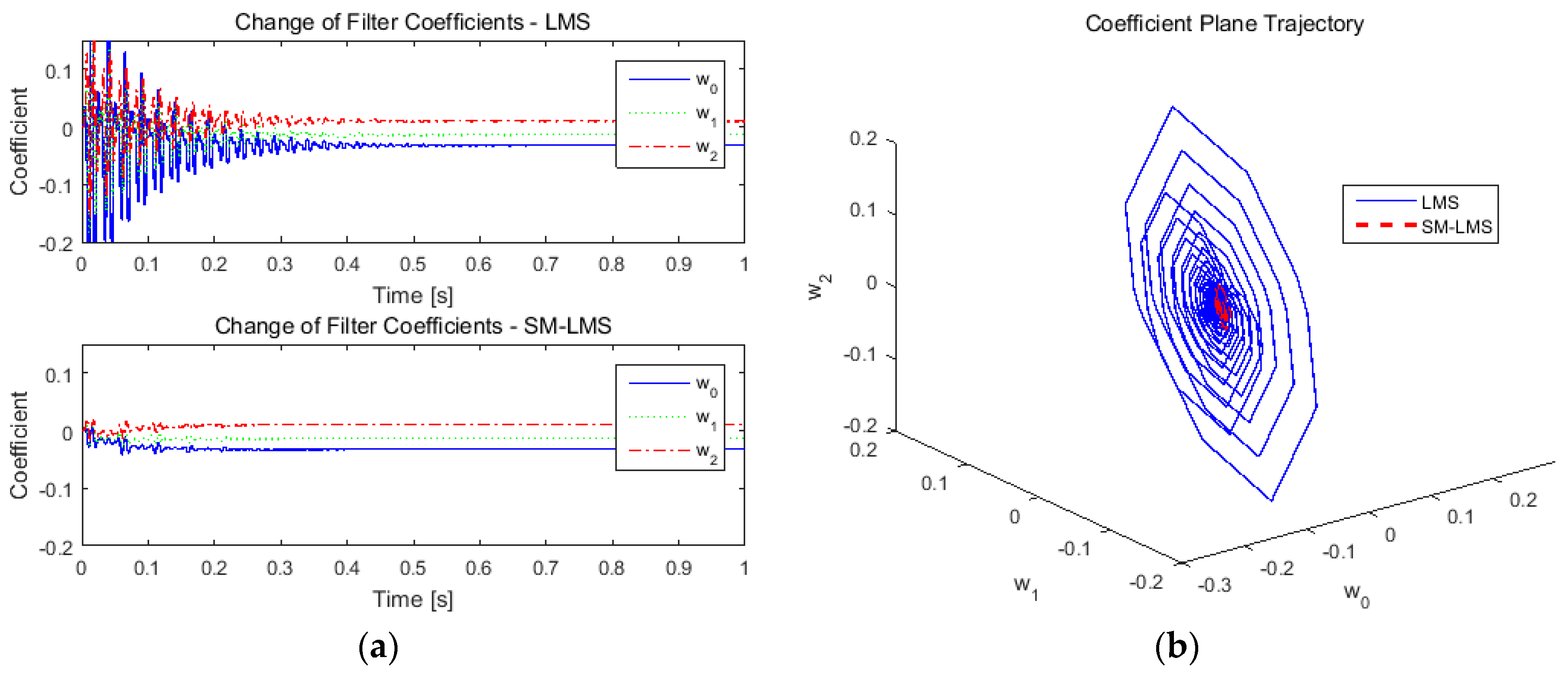
A simple numerical validation was carried out to examine the signal tracking performance of the proposed algorithm under the following conditions: (1) a second-order linear time-invariant (LTI) system with a primary frequency of and damping ratio of ; (2) a finite impulse response (FIR) filter with three coefficients; and (3) a single-frequency sine wave with amplitude , excitation frequency , and no phase (). The control parameters are selected as and . Figure 6a shows the time-domain tracking results with the two algorithms. When the signal has sudden changes in the direction and amount, the conventional LMS algorithm has worse performance than the SM-LMS algorithm, and higher frequency fluctuations are observed compared to the estimation error for both cases, as shown in Figure 6b. It is also important to ensure that the filter weights at steady state approach the same or close values for both algorithms, as shown in Figure 7a. The results show that the sliding mode control only supplements the original LMS algorithm to achieve better optimized convergence without changing its primary characteristics. Figure 5b shows the trajectory of the coefficient plane (the filter weights), and the path to the desired steady state is relatively straight and fast for the SM-LMS. Therefore, changes of the filter weights in the SM-LMS case show superior control without inappropriate system movement.
4. Problem Formulation
A one-dimensional continuous structure was prepared for the validation of the active control strategy. The structure is a thin, aluminum, cantilevered elastic beam with piezoelectric ceramic patches (PZT) attached to both sides. The specific type of PZT material used is PZT-5A and “31” mode has been used for the actuator. It is better for actuator applications for dynamic operating conditions, while it is still good for utilized as sensor applications. The beam can be bent when the ceramic has deformations with applied voltage, which is called a “bimorph”. Figure 8 shows the concept of different types of bimorph structures. The red arrows show the polarization direction, and green arrows indicate the strain direction. Table 1 shows the material properties of the PZT patch.
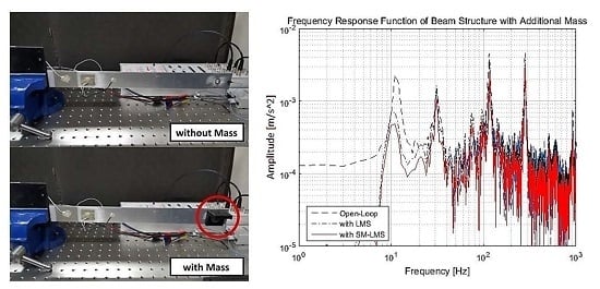
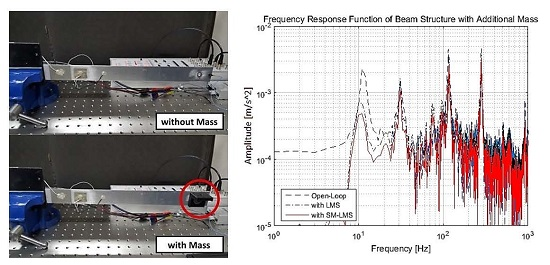
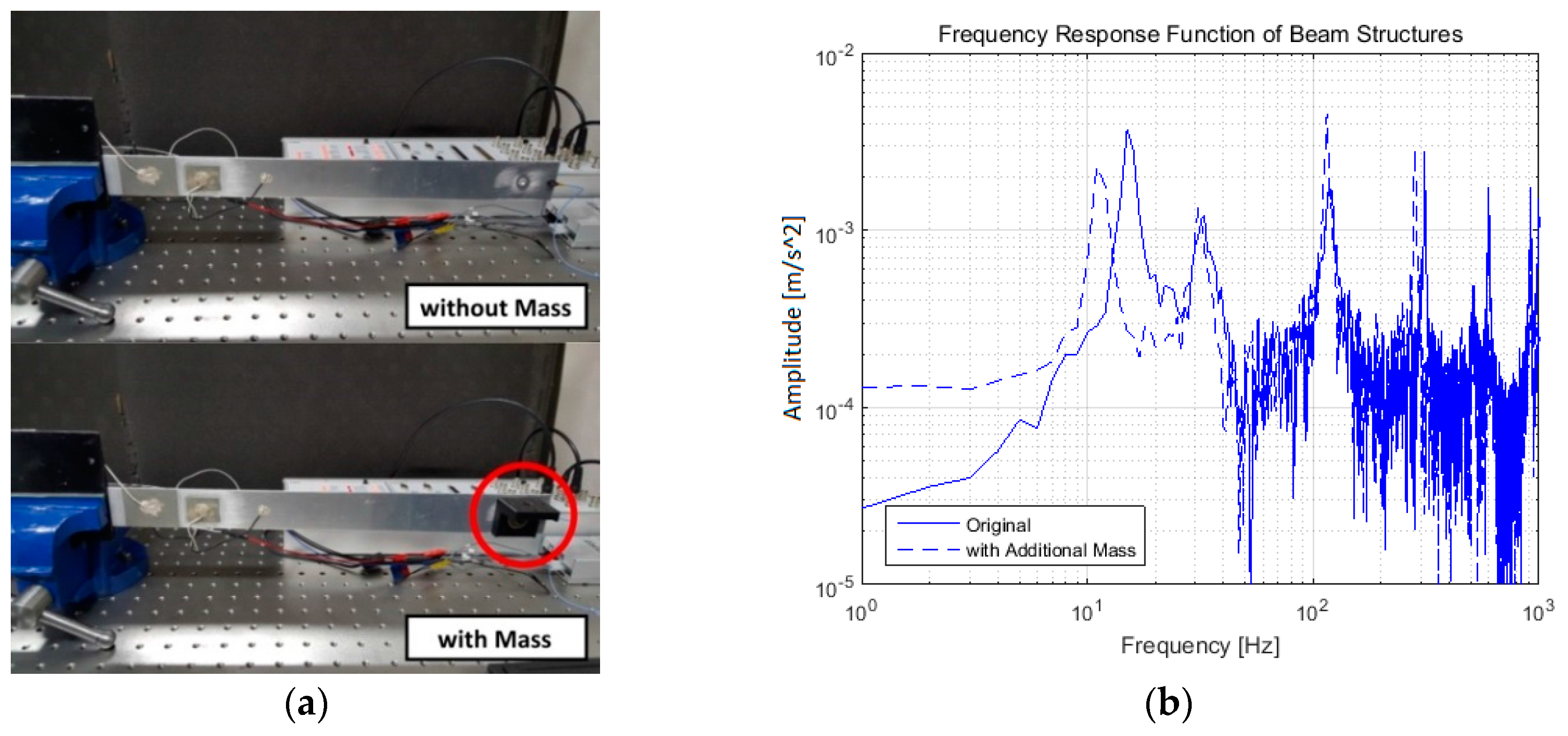
Figure 9 shows a schematic of the experimental setup. Serial bimorph PZT actuators are attached to the surface of the aluminum beam, and an additional small piezoelectric ceramic is attached to one side as a strain sensor for the feedback control system. PZT sensors are selected to check their feasibility for the active vibration control applications. An accelerometer is attached at the tip of the beam as a performance indicator. A bench vise and an electrodynamic shaker are installed on a vibration isolation table, and the whole beam structure is gripped with the vise, resulting clamped-free boundary conditions. The electrodynamic shaker provides impulsive force to the vise, which results in lateral vibration of the beam that has to be mitigated. Additional mass can be attached to the right side of the beam, which works as an impedance change of the structure.
A data acquisition and control system (dSPACE 1104) is used to implement real-time control, and it is connected to a desktop computer with MATLAB/Simulink installed. The designed controllers are uploaded to the dSPACE module after compiling the MATLAB files, and the control system is prepared as follows: (1) signals from the PZT sensor and the accelerometer are acquired by ADC channels and used for the control; and (2) the control input calculated in the dSPACE module is produced from a DAC channel and provided to the PZT actuators after amplification. Figure 10 shows the main components of the experimental setup.
The following frequency response function was obtained from the impact test, and the relationship between the input and output (the transfer function) can be predicted from the results. The objective is to investigate the controller performance with this baseline structure and a modified structure with additional mass, which dramatically changes the structural dynamics and transfer function. Figure 11 compares the frequency response functions of the baseline and the modified structures, and obvious changes in natural frequencies can be observed.
5. System Identification and Notch Filter Design
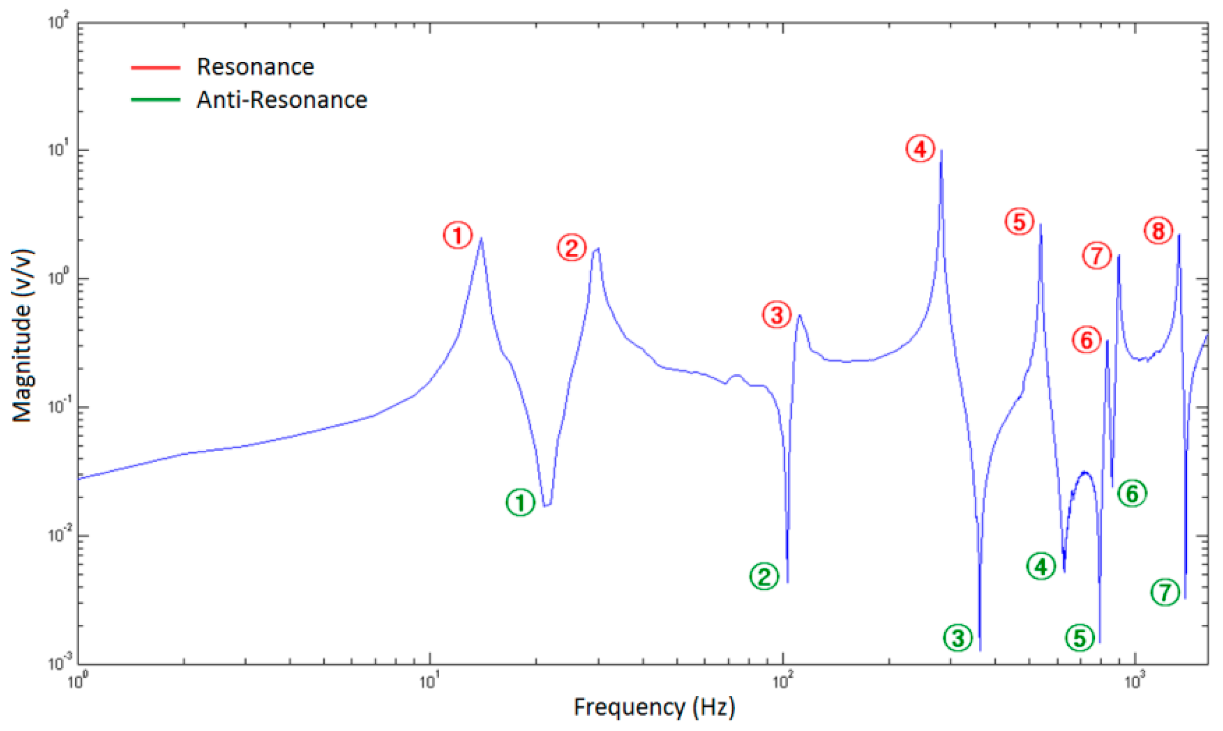
To design an appropriate controller, the structural dynamics of the system should be fully characterized. A frequency-domain system identification method was applied to derive the model of the system. Figure 12 shows the frequency response function of the structural model to be identified. The damping ratio of each peak can be estimated by the quadrature peak picking method. It is a classical method for determining the damping at resonance, and half power (−3 dB) points of each resonance magnitude should be identified.
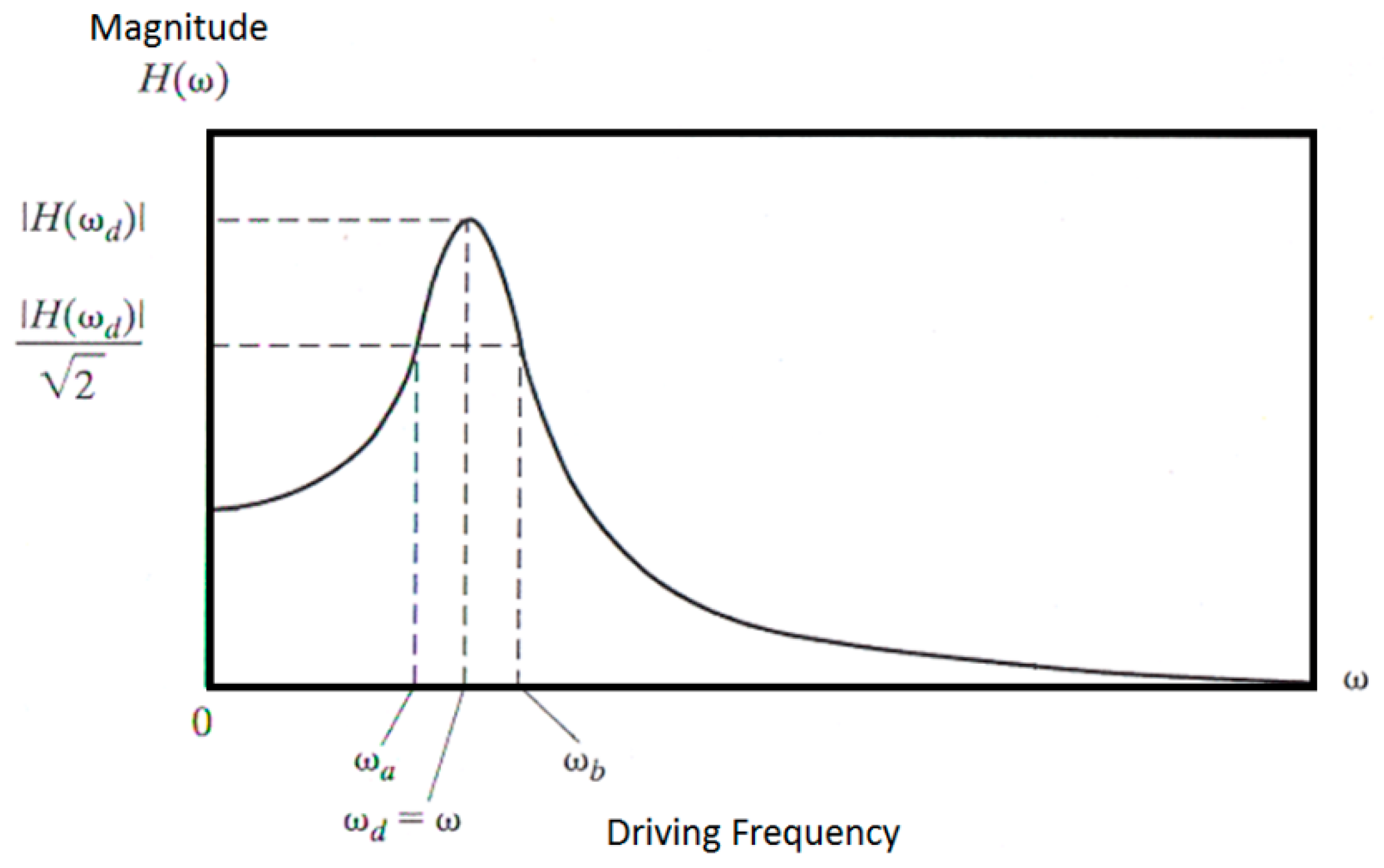
For a particular mode, the damping ratio can be found from Equation (49). Figure 13 illustrates the concept of this method.
The accuracy of this method depends on the frequency resolution used for the measurement, since it determines how accurately the peak magnitude can be measured. For lightly damped structures, high-resolution analysis is required to measure the peak exactly. Consequently, repeated measurements at each resonance frequency are normally required to achieve sufficient accuracy. The obtained resonances are shown in Table 2.
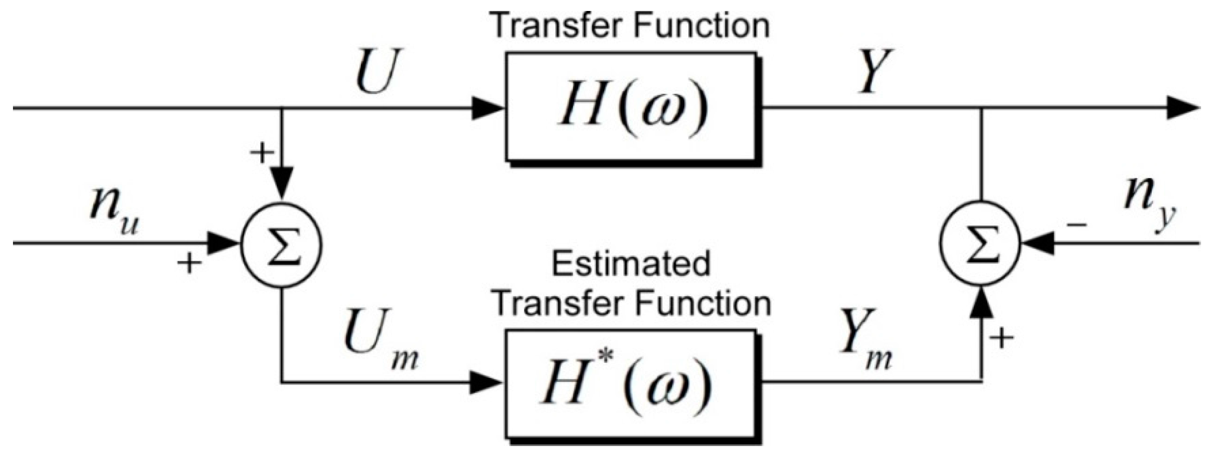
A transfer function can be identified for the object structure based on the frequency response data. The least square estimation of the linear system parameters is presented as a complex-domain formulation [51]. Figure 14 shows a general model of the frequency-domain identification of linear systems. The system is represented by its transfer function , where in the Laplace domain. has a rational form that is extended by a delay term :
The excitation signal is represented by a Fourier series, with complex amplitudes at angular frequencies . The response of the system is . Both the measured input and output complex amplitudes are corrupted by noise terms and , respectively (errors in variables model), which are usually assumed to be Gaussian, uncorrelated between the input and output, and uncorrelated between different frequency points. Based on the above assumptions, a maximum-likelihood estimate of the system parameters is developed in real terms.
The time-domain measurements are transformed into the frequency domain, and the calculated complex input and output amplitudes at selected angular frequencies are and , respectively. The unknown parameters are the unknown coefficients of the numerator and the denominator of the transfer function (Equation (49)), which are collected in the vector . Furthermore, the exact complex input and output amplitudes and are also unknown. The basic equations can be written as follows for the exact values (Equation (50)) and for the noisy observations (Equation (51)):
The maximum-likelihood estimate of the unknown quantities is equivalent to the minimization of the following cost function:
which is subject to the constraints , The upper bar means the complex conjugate, and and are the standard deviations of the input and output, respectively. Using this above methodology, a transfer function with 9 zeros and 11 poles has been identified, which has four major peaks up to around 500 Hz. These four peaks should be attenuated with proper control methods. Figure 15 compares the frequency response functions from the experiment and the system identification, and Equation (53) shows the formulation of the transfer function. This result seems to fit with the experimental results for up to 500 Hz. Figure 15 also shows the root locus for checking which poles are related to each peak. Some parts of the locus go over the right half plane, which indicates instability.
With the identified poles and zeros of the system, notch filters are designed to reduce the amplitude of each peak. A stop band filter (BSF) or a notch filter refers to a band-elimination or blocking filter that exhibits sharp attenuation characteristics in only a specific frequency band. Peak amplitudes can be reduced by adding zeros near poles to maintain the DC gain. Since two zeros are added for each peak, two poles should also be added, which is similar to replacing the damping ratio at each resonance frequency. These are the resonance frequencies and damping ratios of each peak. The filters are derived by maintaining and changing the damping ratio to 0.7. This is done to confirm that an actual solution exists and that enough control authority can be obtained from the actuators for the actual system. Table 3 shows the transfer functions of the notch filters based on Equation (54), in which the original damping ratio replaces the higher damping ratio at each resonance frequency so that the amplitudes at each peak can be attenuated.
As shown in Figure 16, the amplitudes of the peaks are significantly reduced compared to the original system, and the root locus of the filtered system has been changed. The part in the right-hand plane is automatically removed by these filters with the added zeros near poles.
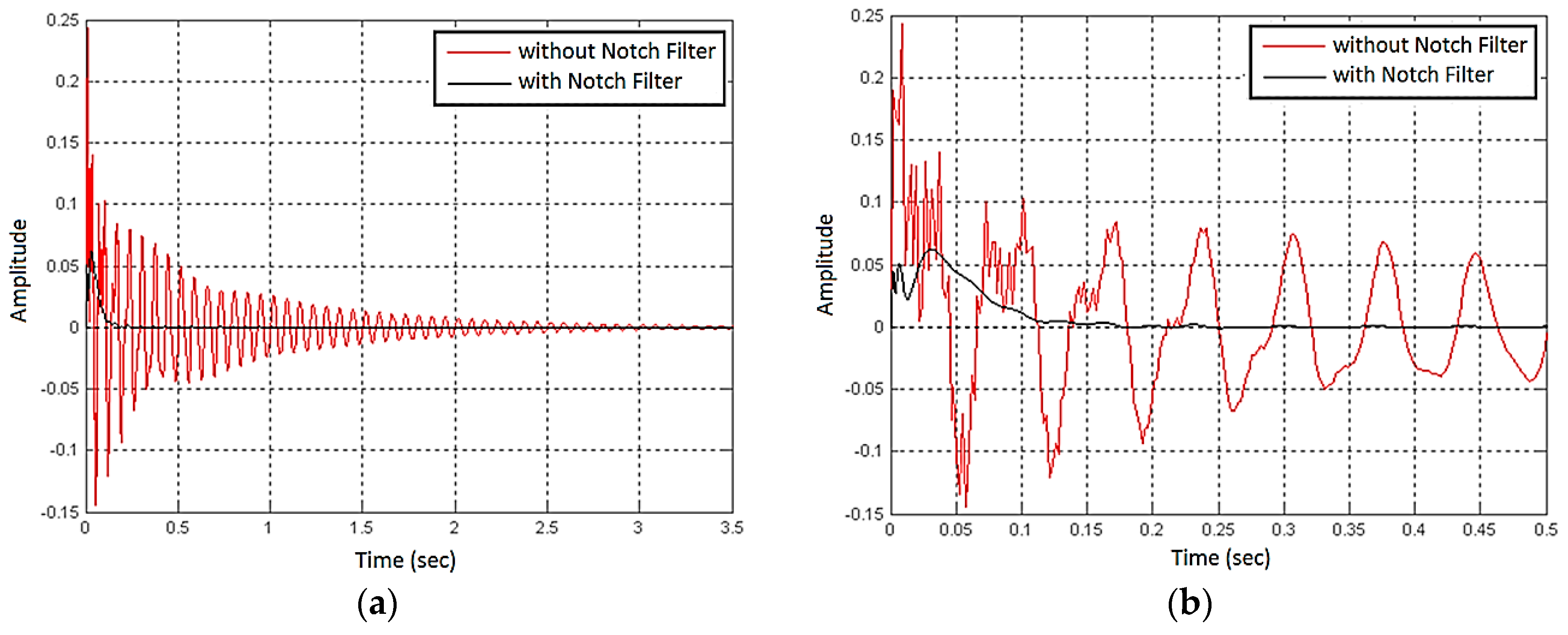
The control results are also described in the time domain. Numerical simulations were conducted with impulse and step inputs to the system. Figure 17 and Figure 18 show the impulse response and the step response of the structure. The notch filters show dramatically reduced vibration amplitudes compared to the case with no control. However, these filters will work on only the baseline structure, assuming that the identified model is accurate.
In a real situation, the exact model of the system cannot be known due to changes in the operational environment, and the plant may vary over time. To incorporate the fact that the plant will change and to highlight the efficacy of the controller, it is assumed that an additional mass (about a 20% increase) is attached to the original system, as mentioned in Section 4.
Since an added mass implies decreased resonance frequencies, a modified transfer function would exist with reduced resonance frequencies for each peak. In the next section, the SM-LMS algorithm’s target-tracking performance is observed for vibration attenuation using the baseline and modified beam structures.
6. Experiments
Several tests were performed with the cantilevered flexible beam. The tests are divided into two cases of vibration reduction control: one for the baseline structure of the beam, and one for a beam with variable mass. The LMS and SM-LMS algorithms are applied to compare the vibration reduction performance. The control parameters were tuned to obtain the best results. Figure 19 shows the control results for the baseline beam structure. The plot on the left indicates the strain change of the aluminum beam in the time domain from the PZT sensor outputs. Note that the vibration stops in 0.2 to 0.3 s with LMS and SM-LMS, whereas it takes longer than 1 s to stop without a controller. The plot on the right compares the frequency response plots between open-loop and closed-loop cases, and some amplitude reductions can be seen for each peak frequency.
After 0.3 s, the vibration amplitudes with both control algorithms are very similar, but LMS shows worse vibration isolation performance than SM-LMS. The frequency response shows a more obvious performance difference between the two methods, as shown in Table 4.
There is excellent attenuation of mode 1 and slight attenuation of mode 2 with LMS, while higher frequencies show slight amplifications. SM-LMS shows excellent attenuation of modes 1 and 2 and slight attenuation of mode 4, while mode 3 shows slight amplification. At every peak, the difference in attenuated amplitude between the two methods is about 3 to 5 dBs. The amplitudes of 1st, 2nd, and 4th modal frequencies are reduced, and the 3rd modal frequency has some spill-over with SM-LMS. However, with LMS, the 3rd and 4th peaks have spillovers, and the amounts are higher than in the case with SM-LMS. When observing the vibration level in broadband, the SM-LMS shows better vibration isolation performance, thus reducing the overall RMS value.
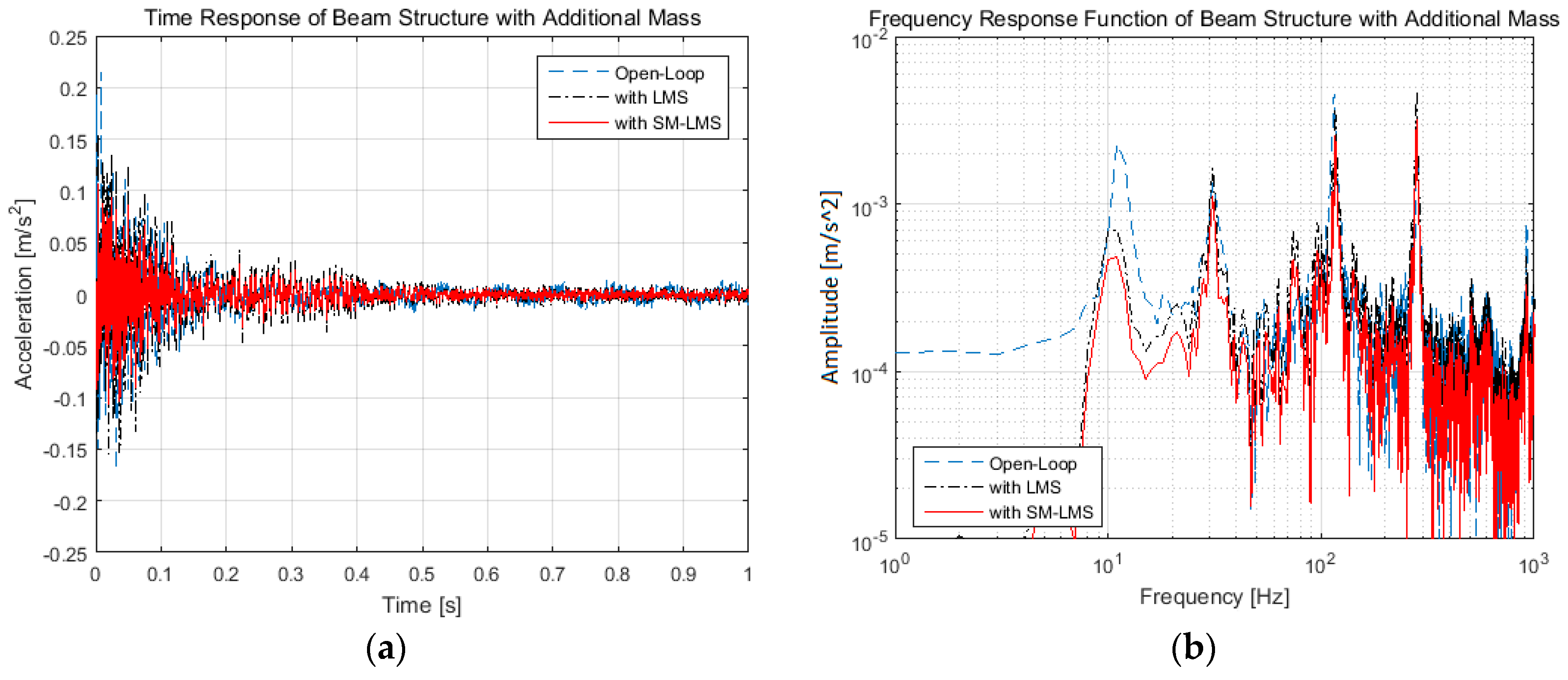
Next, to incorporate the fact that the plant will change and to highlight the efficacy of the controller, an additional mass is attached to the original system (increasing the total weight by about a 20%). A bracket is fastened near the tip of the beam, as shown in Figure 11. Since an added mass implies decreased resonance frequencies, a modified frequency response with reduced resonance frequencies for each peak is obtained to measure the performance of the controller in these cases. Note that the SM-LMS is not related to the original structural dynamics and can make the system have desired dynamics. Moreover, the parameters of the SM-LMS used for the baseline structures are maintained for this case of control in order to observe the robustness of the controller.
Again, the time-domain responses caused by impulsive disturbances show significant reduction visible, as shown in Figure 20. Furthermore, the amplitudes of each resonance peak and other frequencies are decreased, regardless of the significant change in the plant dynamics. Similarly, the vibration stops in 0.4 to 0.5 s with LMS and SM-LMS, whereas it takes longer than 1 s without a controller. The plot on the right compares the frequency response between the open-loop and closed-loop cases, in which some amplitude reductions can be seen for each peak frequency.
After 0.5 s, the vibration amplitudes for both control algorithms are very similar, but LMS shows worse vibration isolation performance than SM-LMS. The frequency response shows a more obvious performance difference between the two methods, as indicated in Table 5. LMS shows excellent attenuation of mode 1 but has very little effect on higher modes. SM-LMS shows excellent attenuation of mode 1 and slight attenuation of modes 2 and 3, while mode 4 shows very slight amplification. At every peak, the difference in attenuated amplitude between the two methods is about 2 to 3 dBs. The amplitudes of the 1st, 2nd, and 3rd modal frequencies are reduced, and the 4th modal frequency has some spill-over with SM-LMS. However, with LMS, the 2nd and 4th peaks have spillovers, and the amounts are higher than in the case with SM-LMS. When observing the vibration level in broadband, the SM-LMS shows better vibration isolation performance, thus showing a reduced overall RMS value, although it is 1.1 dB lower than the baseline case.
As shown in the simulation results, the time-domain responses caused by impulsive disturbances are significantly reduced, and the amplitude of each resonance peak is nearly flattened. These results verify that the SM-LMS method can reduce the vibration of the cantilevered beam considerably, even though the structural dynamics is dramatically changed with the additional impedance.
7. Conclusions and Future Work
An enhanced LMS algorithm has been proposed and applied to an adaptive digital filtering system combined with sliding mode control. The method benefits from the nonlinear control technique inside the control system structure for better adaptability and tracking performance. This adaptive filtering system was used for the vibration reduction and control of a continuous smart structure with piezoelectric patches attached to it. The SM-LMS method allows for significant and robust vibration reduction for not only the original structure, but also for a beam with modified dynamics. Thus, it can be a good solution for reducing the vibration of structures with unknown dynamics.
The contributions of this research are summarized as: First, the proposed control system has improved stability, robustness, and capability to manage signals with multiple spectra with increasing complexity and frequency of components to be controlled in the output of the disturbance plant. Numerical analyses demonstrated that the method has adequate tracking performance. Second, a smart structure with piezoelectric patches was constructed and its dynamic model has been identified with frequency domain identification method; third, a conventional control method has been validated numerically in the case of active vibration control and showed limitations. Third, the method was validated for the original structure and a modified structure. The controller had acceptable tracking performance in both cases.
This work could be validated with several real-world applications in active vibration control, such as vehicle vibration reduction and vibration attenuation for engineering structures. In addition, a hybrid controller could be proposed to control two or more directions simultaneously for realistic applications by effectively managing an extensive range of multi-spectral signals. Self-sensing actuator could be implemented with one PZT material, which acts as sensor and actuator simultaneously. Intelligent control methods such as neural networks could also be more adaptive and robust to changeable system dynamics.
Acknowledgments
This paper was supported by the National Research Foundation of Korea (NRF) grant funded by the government of Korea (Ministry of Science, ICT & Future Planning) (No. 2016R1C1B1010888) as well as by the 2017 Yeungnam University Research Grant (217A380020).
Author Contributions
Byeongil Kim and Jong-yun Yoon initiated and developed the ideas related to this research work. Byeongil Kim and Jong-yun Yoon developed novel methods, derived relevant formulations, and carried out performance analyses and numerical analyses. Byeongil Kim wrote the paper draft under Jong-yun Yoon’s guidance and Byeongil Kim finalized the paper.
Conflicts of Interest
The authors declare no conflict of interest.
References
- Bianchini, E. Active vibration control of automotive like panels. In Proceedings of the 2008 SAE Brasil Noise Vibration Conference, Florianópolis, Brazil, 30 March–1 April 2008. [Google Scholar]
- Raju, B.B.; Bianchini, E.; Arata, J.; Roylance, M. Improved performance of a baffle-less automotive muffler using piezoelectric materials. In Proceedings of the SAE 2005 Noise Vibration Conference and Exhibition, Traverse City, MI, USA, 16–19 May 2005. [Google Scholar]
- Wolff, K.; Lahey, H.P.; Nussmann, C.; Nehl, J.; Wimmel, R.; Siebald, H.; Fehren, H.; Redaelli, M.; Naake, A. Active noise cancellation at powertrain oil pan. In Proceedings of the SAE 2007 Noise Vibration Conference and Exhibition, St. Charles, IL, USA, 15–17 May 2007. [Google Scholar]
- Rao, A.K.; Natesan, K.; Bhat, S.M.; Ganguli, R. Experimental demonstration of H-inf control based active vibration suppression in composite fin-tip of aircraft using optimally placed piezoelectric patch actuators. J. Intell. Mater. Syst. Struct. 2008, 19, 651–669. [Google Scholar] [CrossRef]
- Shevtsov, S.; Soloviev, A.; Acopyan, V.; Samochenko, I. Helicopter rotor blade vibration control on the basis of active/passive piezoelectric damping approach. In Proceedings of the PHYSCON, Catania, Italy, 1–4 September 2009. [Google Scholar]
- Song, Z.G.; Li, F.M. Active aeroelastic flutter analysis and vibration control of supersonic beams using the piezoelectric actuator/sensor pairs. Smart Mater. Struct. 2011, 20, 055013. [Google Scholar] [CrossRef]
- Sun, H.; Yang, Z.; Li, K.; Li, B.; Xie, J.; Wu, D.; Zhang, L. Vibration suppression of a hard disk driver actuator arm using piezoelectric shunt damping with a topology-optimized PZT transducer. Smart Mater. Struct. 2009, 18, 065010. [Google Scholar] [CrossRef]
- Lim, Y.Y.; Soh, C.K. Fatigue life estimation of a 1D aluminum beam under mode-I loading using the electromechanical impedance technique. Smart Mater. Struct. 2011, 20, 125001. [Google Scholar] [CrossRef]
- Wu, N.; Wang, Q. Repair of vibrating delaminated beam structures using piezoelectric patches. Smart Mater. Struct. 2010, 19, 035027. [Google Scholar] [CrossRef]
- Makihara, K. Energy-efficiency enhancement and displacement-offset elimination for hybrid vibration control. Smart Struct. Syst. 2012, 10, 193–207. [Google Scholar] [CrossRef]
- Bruant, I.; Proslier, L. Improved active control of a functionally graded material beam with piezoelectric patches. J. Vib. Control 2015, 21, 2059–2080. [Google Scholar] [CrossRef]
- Silva, L.P.; Larbi, L.; Deu, J.F. Topology optimization of shunted piezoelectric elements for structural vibration reduction. J. Intell. Mater. Syst. Struct. 2015, 26, 1219–1235. [Google Scholar] [CrossRef]
- Li, K.; Li, S.; Zhao, D. Identification and suppression of vibrational energy in stiffened plates with cutouts based on visualization techniques. Struct. Eng. Mech. 2012, 43, 395–410. [Google Scholar] [CrossRef]
- Shi, Z.; Li, J.; Yao, R. Solution modification of a piezoelectric bimorph cantilever under loads. J. Intell. Mater. Syst. Struct. 2015, 26, 2028–2041. [Google Scholar] [CrossRef]
- Tehrani, M.G.; Kalkowski, M.K. Active control of parametrically excited systems. J. Intell. Mater. Syst. Struct. 2016, 27, 1218–1230. [Google Scholar] [CrossRef]
- Alaimo, A.; Milazzo, A.; Orlando, C. A smart composite-piezoelectric one-dimensional finite element model for vibration damping analysis. J. Intell. Mater. Syst. Struct. 2016, 27, 1362–1375. [Google Scholar] [CrossRef]
- Kashani, R.; Mazdeh, A.; Orzechowski, J. Shunt piezo damping of a radiating panel. In Proceedings of the 2001 Noise Vibration Conference, Traverse City, MI, USA, 5–8 March 2001. [Google Scholar]
- Trindade, M.A.; Maio, C.E.B. Multimodal passive vibration control of sandwich beams with shunted shear piezoelectric materials. Smart Mater. Struct. 2008, 17, 055015. [Google Scholar] [CrossRef]
- Ji, H.; Qiu, J.; Badel, A.; Zhu, K. Semi-active vibration control of a composite beam using an adaptive SSDV approach. J. Intell. Mater. Syst. Struct. 2009, 20, 401–412. [Google Scholar]
- Beck, B.S.; Cunefare, K.A.; Ruzzene, M.; Collet, M. Experimental analysis of a cantilever beam with a shunted piezoelectric periodic array. J. Intell. Mater. Syst. Struct. 2011, 22, 177–1187. [Google Scholar] [CrossRef]
- Mahmoodi, S.N.; Ahmadian, M.; Inman, D.J. Adaptive modified positive position feedback for active vibration control of structures. J. Intell. Mater. Syst. Struct. 2010, 21, 571–580. [Google Scholar] [CrossRef]
- Fanson, J.L.; Caughey, T.K. Positive position feedback control for large space structures. AIAA J. 1990, 28, 717–724. [Google Scholar] [CrossRef]
- Mahmoodi, S.N.; Ahmadian, M. Modified acceleration feedback for active vibration control of aerospace structures. Smart Mater. Struct. 2010, 19, 065015. [Google Scholar] [CrossRef]
- Preumont, A.; Loix, N.; Malaise, D.; Lecrenier, O. Active damping of optical test benches with acceleration feedback. Machine Vib. 1993, 2, 119–124. [Google Scholar]
- Yoon, H.S.; Washington, G. Active vibration confinement of flexible structures using piezoceramic patch actuators. J. Intell. Mater. Syst. Struct. 2008, 19, 145–155. [Google Scholar] [CrossRef]
- Nguyen, P.B.; Choi, S.B. Open-loop position tracking control of a piezoceramic flexible beam using a dynamic hysteresis compensator. Smart Mater. Struct. 2010, 19, 125008. [Google Scholar] [CrossRef]
- Sethi, V.; Song, G. Multimodal vibration control of a flexible structure using piezoceramic sensor and actuator. J. Intell. Mater. Syst. Struct. 2008, 19, 573–582. [Google Scholar] [CrossRef]
- Mirzaee, E.; Eghtesad, M.; Fazelzadeh, S.A. Trajectory tracking and active vibration suppression of a smart Single-Link flexible arm using a composite control design. Smart Struct. Syst. 2011, 7, 103–116. [Google Scholar] [CrossRef]
- Escareno, J.A.; Rakotondrabe, M.; Habineza, D. Backstepping-based robust-adaptive control of a nonlinear 2-DOF piezoactuator. Control Eng. Pract. 2015, 41, 57–71. [Google Scholar] [CrossRef]
- Canahuire, R.; Serpa, A.L. Reduced order H-inf controller design for vibration control using genetic algorithms. J. Vib. Control 2017, 23, 1693–1707. [Google Scholar] [CrossRef]
- Kim, B.; Washington, G.N.; Singh, R. Control of incommensurate sinusoids using enhanced adaptive filtering algorithm based on sliding mode approach. J. Vib. Control 2013, 19, 1265–1280. [Google Scholar] [CrossRef]
- Kim, B.; Washington, G.N.; Yoon, H.S. Control and hysteresis reduction in prestressed curved unimorph actuators using model predictive control. J. Intell. Mater. Syst. Struct. 2014, 25, 290–307. [Google Scholar] [CrossRef]
- Kuo, S.M.; Morgan, D.R. Active Noise Control Systems: Algorithms and DSP Implementations; John Wiley & Sons: New York, NY, USA, 1996. [Google Scholar]
- Widrow, B.; Stearns, S.D. Adaptive Signal Processing; Prentice-Hall: Englewood Cliffs, NJ, USA, 1985. [Google Scholar]
- Clark, R.L.; Saunders, W.R.; Gibbs, G.P. Adaptive Structures: Dynamics and Control; John Wiley&Sons: New York, NY, USA, 1998. [Google Scholar]
- Widrow, B.; Glover, J.R.; McCool, J.M.; Kaunitz, J.; Williams, C.S.; Hearn, R.H.; Zeidler, J.R.; Dong, E.; Goodlin, R.C. Adaptive noise cancelling: Principles and applications. Proc. IEEE 1975, 63, 1692–1716. [Google Scholar] [CrossRef]
- Bai, M.R.; Luo, W. DSP implementation of an active bearing mount for rotors using hybrid control. ASME J. Vib. Acoust. 2000, 122, 420–428. [Google Scholar] [CrossRef]
- Adeli, H.; Kim, H. Hybrid feedback-least mean square algorithm for structural control. J. Struct. Eng. 2004, 130, 120–127. [Google Scholar] [CrossRef]
- Bouchard, M.; Paillard, B. An alternative feedback structure for the adaptive active control of periodic and time-varying periodic disturbances. J. Sound Vib. 1998, 210, 517–527. [Google Scholar] [CrossRef]
- Pan, M.; Wei, W. Adaptive focusing control of DVD drives in vehicle systems. J. Vib. Control 2006, 12, 1239–1250. [Google Scholar] [CrossRef]
- Sabah, Y.; Okuma, M.; Okubo, M. Implementation of single and multiple adaptive step-size algorithm to ANC. ASME J. Vib. Acoust. 2008, 130, 129–132. [Google Scholar] [CrossRef]
- Hao, L.; Li, Z. Modeling and adaptive inverse control of hysteresis and creep in ionic polymer-metal composite actuators. Smart Mater. Struct. 2010, 19, 025014. [Google Scholar] [CrossRef]
- Carnahan, J.J.; Richards, C.M. A modification to filtered-X LMS control for airfoil vibration and flutter suppression. J. Vib. Control 2008, 14, 831–848. [Google Scholar] [CrossRef]
- Akhtar, M.T.; Mitsuhashi, W. Improving performance of FxLMS algorithm for active noise control of impulsive noise. J. Sound Vib. 2009, 327, 647–656. [Google Scholar] [CrossRef]
- Zhang, Z.; Hu, F.; Wang, J. On saturation suppression in adaptive vibration control. J. Sound Vib. 2010, 329, 1209–1214. [Google Scholar] [CrossRef]
- Kuo, S.M.; Gupta, A.; Mallu, S. Development of adaptive algorithm for active sound quality control. J. Sound Vib. 2007, 299, 12–21. [Google Scholar] [CrossRef]
- Zhou, D.F.; Li, J.; Hansen, C.H. Application of least mean square algorithm to suppression of maglev track induced self-excited vibration. J. Sound Vib. 2011, 330, 5791–5810. [Google Scholar] [CrossRef]
- Young, K.D.; Utkin, V.I.; Ozguner, U. A control engineer’s guide to sliding mode control. IEEE Trans. Control Syst. Technol. 1999, 7, 328–342. [Google Scholar] [CrossRef]
- Utkin, V.; Guldner, J.; Shi, J. Sliding Mode Control in Electromechanical Systems; Taylor & Francis: Philadelphia, PA, USA, 1999. [Google Scholar]
- Slotine, J.J.; Sastry, S.S. Tracking control of nonlinear systems using sliding surfaces with application to robot manipulators. Int. J. Control 1983, 38, 465–492. [Google Scholar] [CrossRef]
- Kollar, I. On Frequency-Domain Identification of Linear Systems. IEEE Trans. Inst. Meas. 1993, 42, 2–6. [Google Scholar] [CrossRef]
Figure 1.
Typical adaptive digital filtering system.
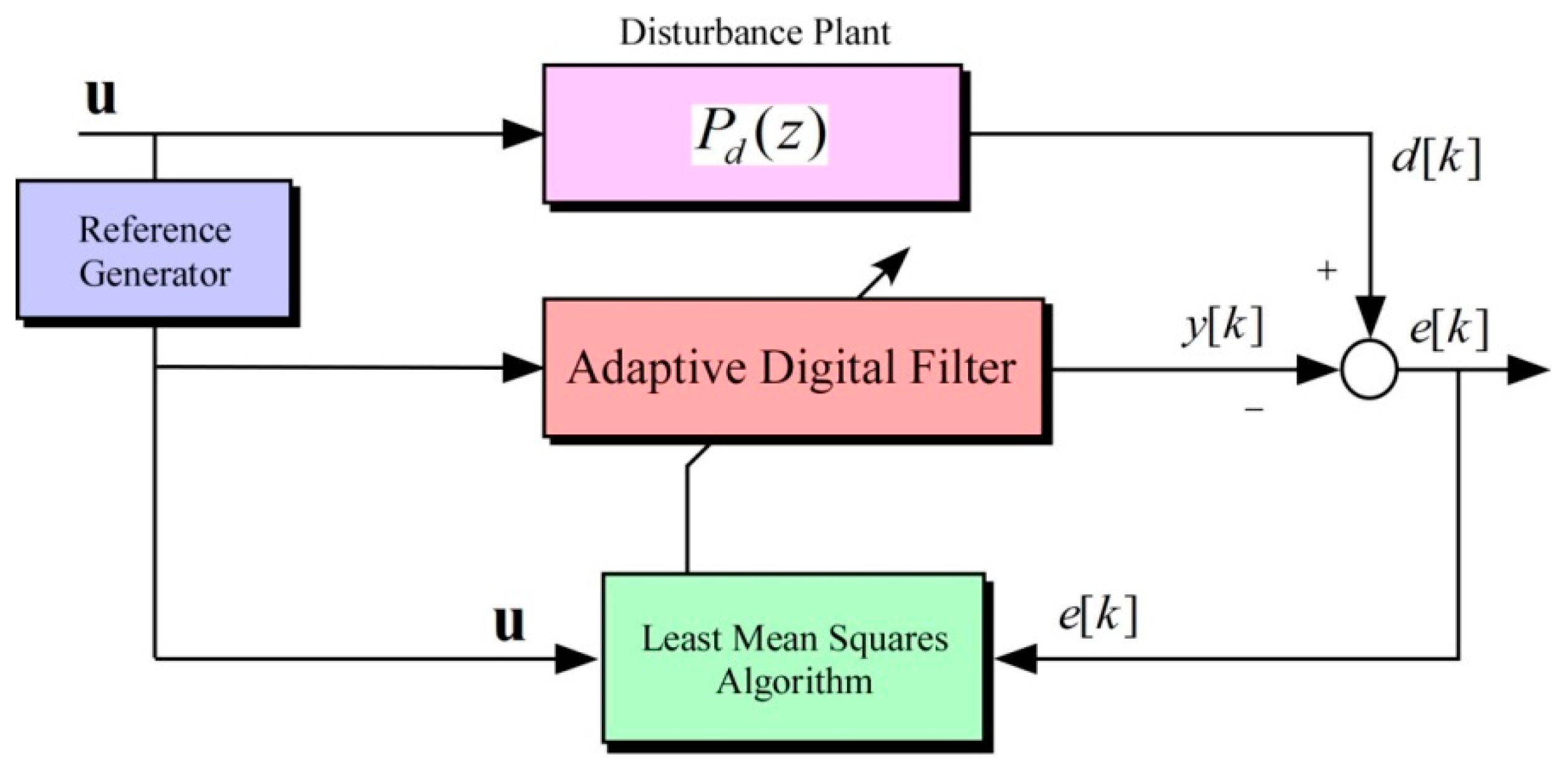
Figure 2.
Filtered-X least mean square algorithm.
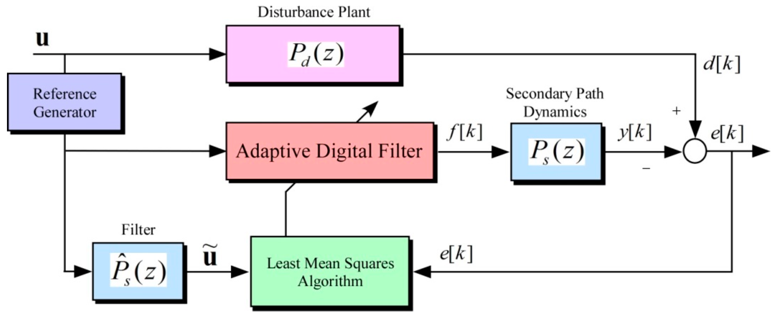
Figure 3.
Phase trajectory in sliding mode: (a) ideal sliding mode; and (b) real sliding mode.

Figure 4.
Proposed sliding mode least mean squares control (SM-LMS) method.
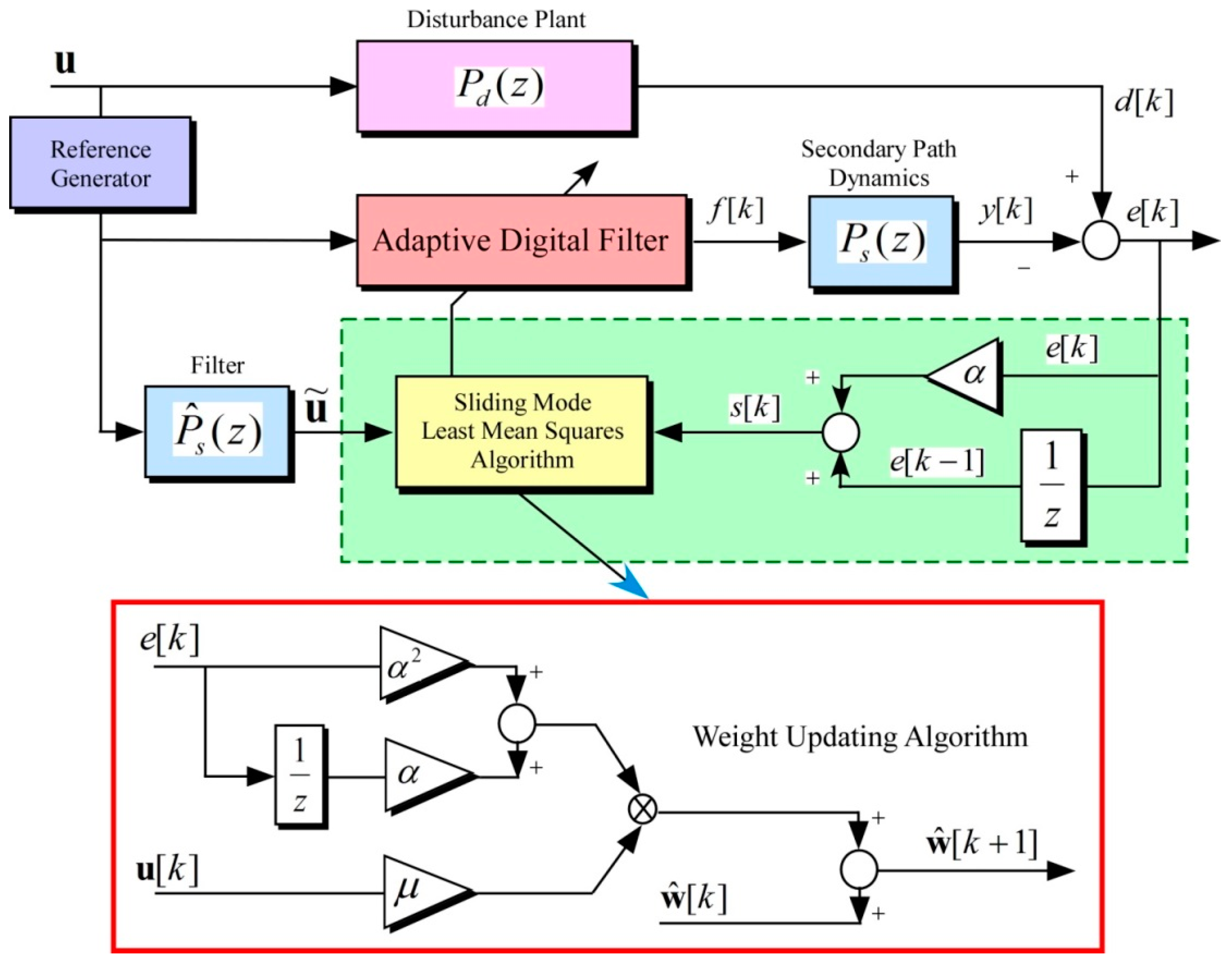
Figure 5.
Error surface illustration for: (a) the conventional LMS method; and (b) SM-LMS.
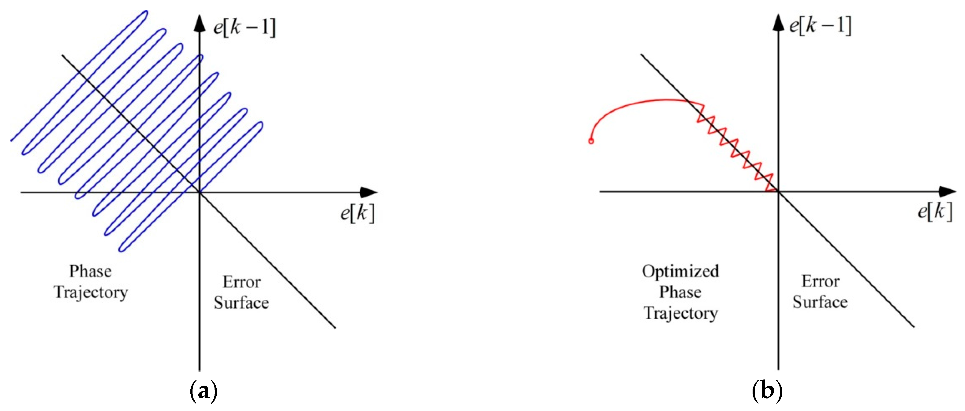
Figure 6.
Control of a single sinusoid at 120 Hz in the time domain: (a) predicted with least mean squares and sliding mode least mean squares (Key: ![Applsci 07 00750 i001]() , original signal;
, original signal; ![Applsci 07 00750 i002]() , filter output); and (b) predicted estimation error (Key:
, filter output); and (b) predicted estimation error (Key: ![Applsci 07 00750 i003]() , with least mean squares;
, with least mean squares; ![Applsci 07 00750 i004]() , with sliding mode least mean squares).
, with sliding mode least mean squares).
 , original signal;
  , filter output); and (b) predicted estimation error (Key:
  , with least mean squares;
  , with sliding mode least mean squares).
Figure 6.
Control of a single sinusoid at 120 Hz in the time domain: (a) predicted with least mean squares and sliding mode least mean squares (Key: ![Applsci 07 00750 i001]() , original signal;
, original signal; ![Applsci 07 00750 i002]() , filter output); and (b) predicted estimation error (Key:
, filter output); and (b) predicted estimation error (Key: ![Applsci 07 00750 i003]() , with least mean squares;
, with least mean squares; ![Applsci 07 00750 i004]() , with sliding mode least mean squares).
, with sliding mode least mean squares).
, original signal; , filter output); and (b) predicted estimation error (Key: , with least mean squares; , with sliding mode least mean squares).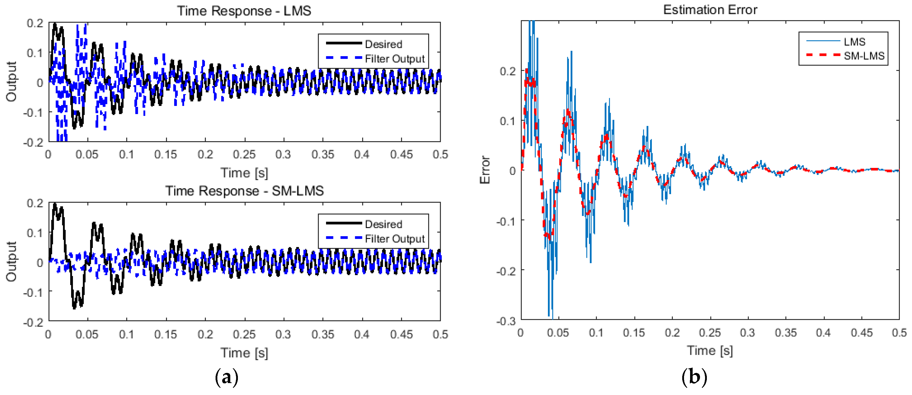
Figure 7.
Comparison of least mean squares and sliding mode least mean squares: (a) change in filter coefficients (Key: ![Applsci 07 00750 i005]() , w0;
, w0; ![Applsci 07 00750 i006]() , w1;
, w1; ![Applsci 07 00750 i007]() , w2); and (b) comparison of trajectories in the plane of filter coefficients (Key:
, w2); and (b) comparison of trajectories in the plane of filter coefficients (Key: ![Applsci 07 00750 i003]() , least mean squares;
, least mean squares; ![Applsci 07 00750 i004]() , sliding mode least mean squares).
, sliding mode least mean squares).
 , w0;
, w0;  , w1;
, w1;  , w2); and (b) comparison of trajectories in the plane of filter coefficients (Key: , least mean squares; , sliding mode least mean squares).
Figure 7.
Comparison of least mean squares and sliding mode least mean squares: (a) change in filter coefficients (Key: ![Applsci 07 00750 i005]() , w0;
, w0; ![Applsci 07 00750 i006]() , w1;
, w1; ![Applsci 07 00750 i007]() , w2); and (b) comparison of trajectories in the plane of filter coefficients (Key:
, w2); and (b) comparison of trajectories in the plane of filter coefficients (Key: ![Applsci 07 00750 i003]() , least mean squares;
, least mean squares; ![Applsci 07 00750 i004]() , sliding mode least mean squares).
, sliding mode least mean squares).
, w0; , w1; , w2); and (b) comparison of trajectories in the plane of filter coefficients (Key: , least mean squares; , sliding mode least mean squares).
Figure 8.
Bimorph concept: (a) parallel bimorph; and (b) serial bimorph.
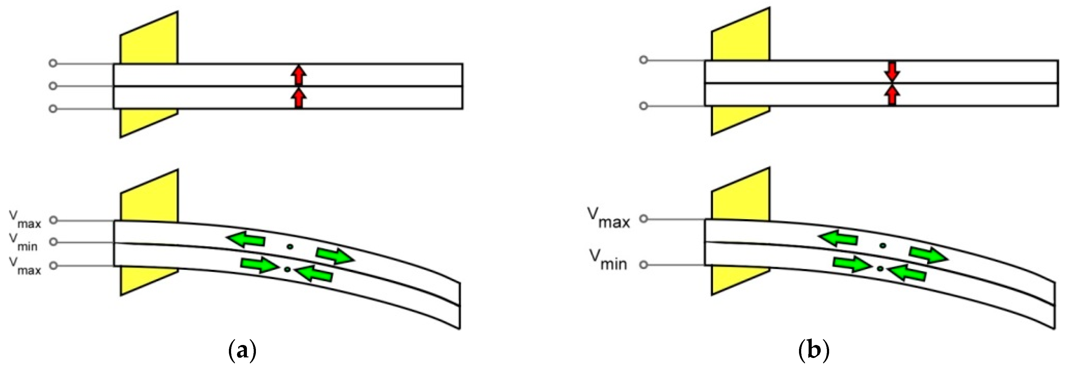
Figure 9.
Schematic of experimental setup.
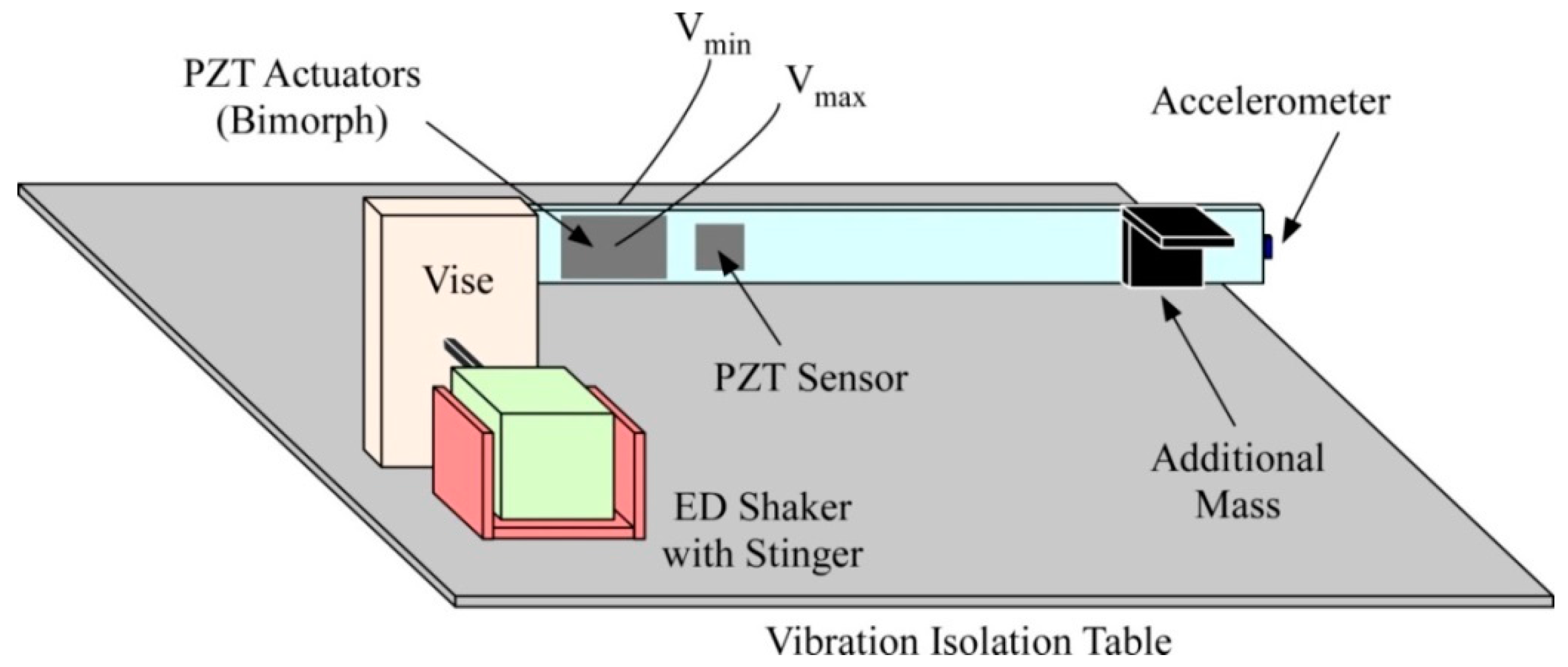
Figure 10.
Experimental setup.
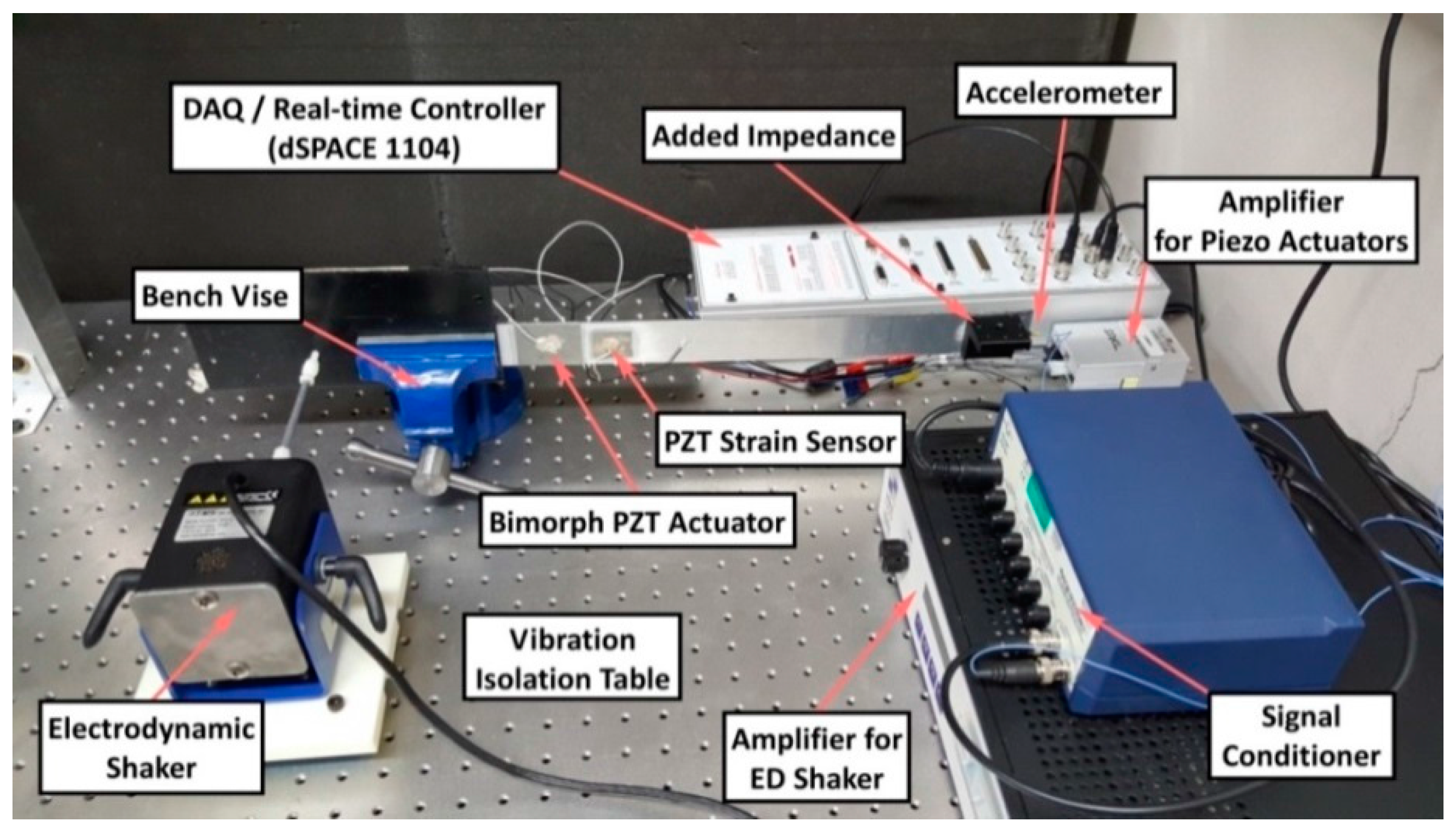
Figure 11.
Frequency response function of beam structure: (a) two different configurations; and (b) comparison of frequency response function.
Figure 11.
Frequency response function of beam structure: (a) two different configurations; and (b) comparison of frequency response function.

Figure 12.
Frequency response function of the structural model to be identified.

Figure 13.
Quadrature peak picking method.

Figure 14.
Frequency-domain identification of linear systems.

Figure 15.
Comparison of: (a) frequency response functions; and (b) root locus.
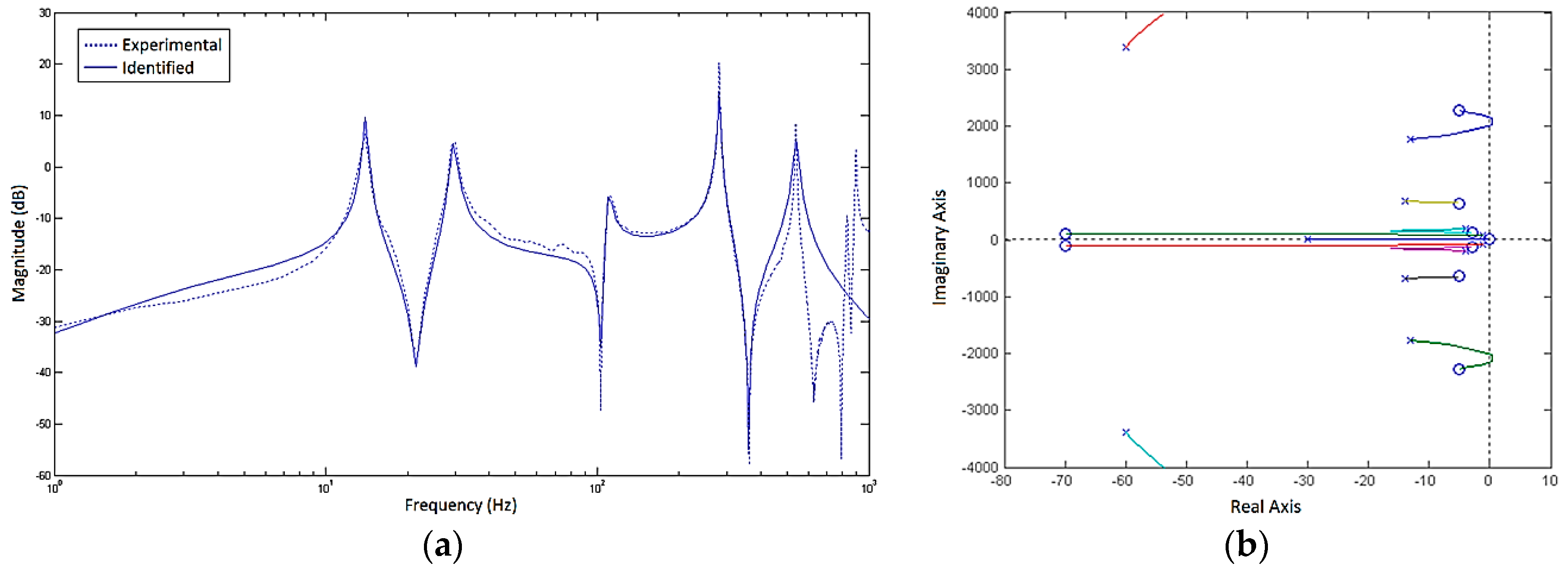
Figure 16.
Notch filter control result: (a) frequency response functions; and (b) changed root locus.
Figure 16.
Notch filter control result: (a) frequency response functions; and (b) changed root locus.
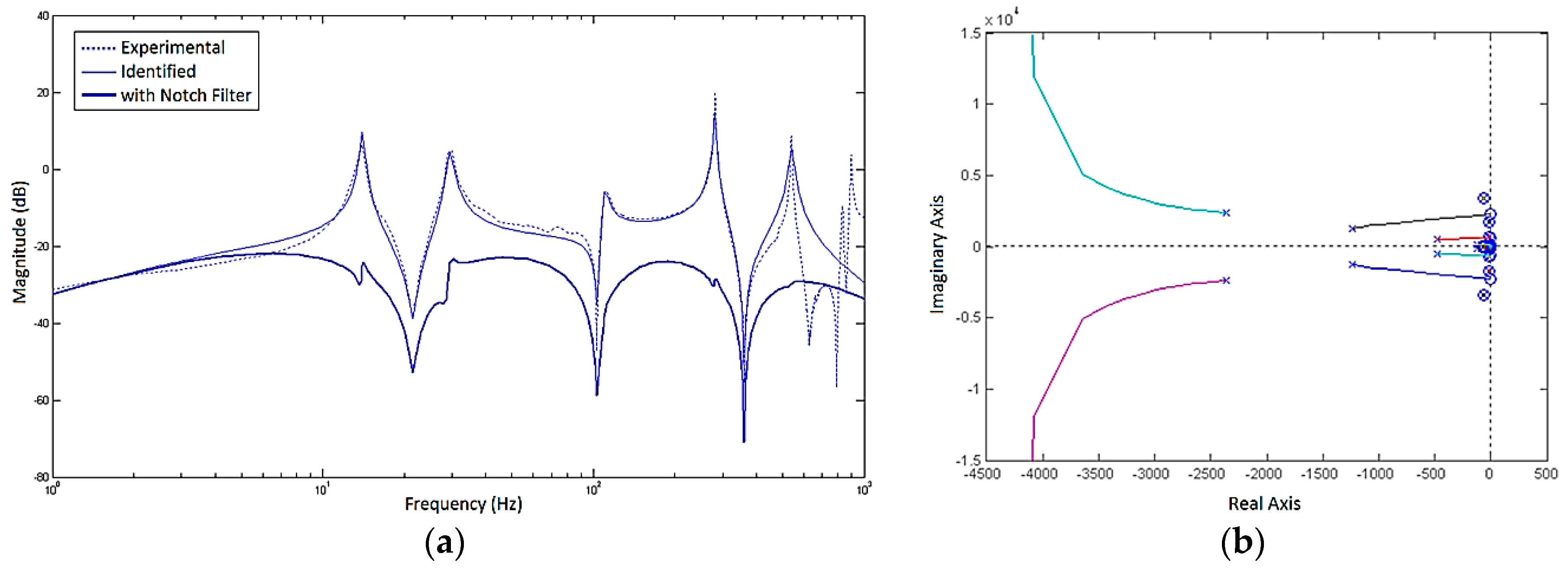
Figure 17.
Notch filter control result: (a) tracking error of impulse response; and (b) zoomed plot of (a).
Figure 17.
Notch filter control result: (a) tracking error of impulse response; and (b) zoomed plot of (a).
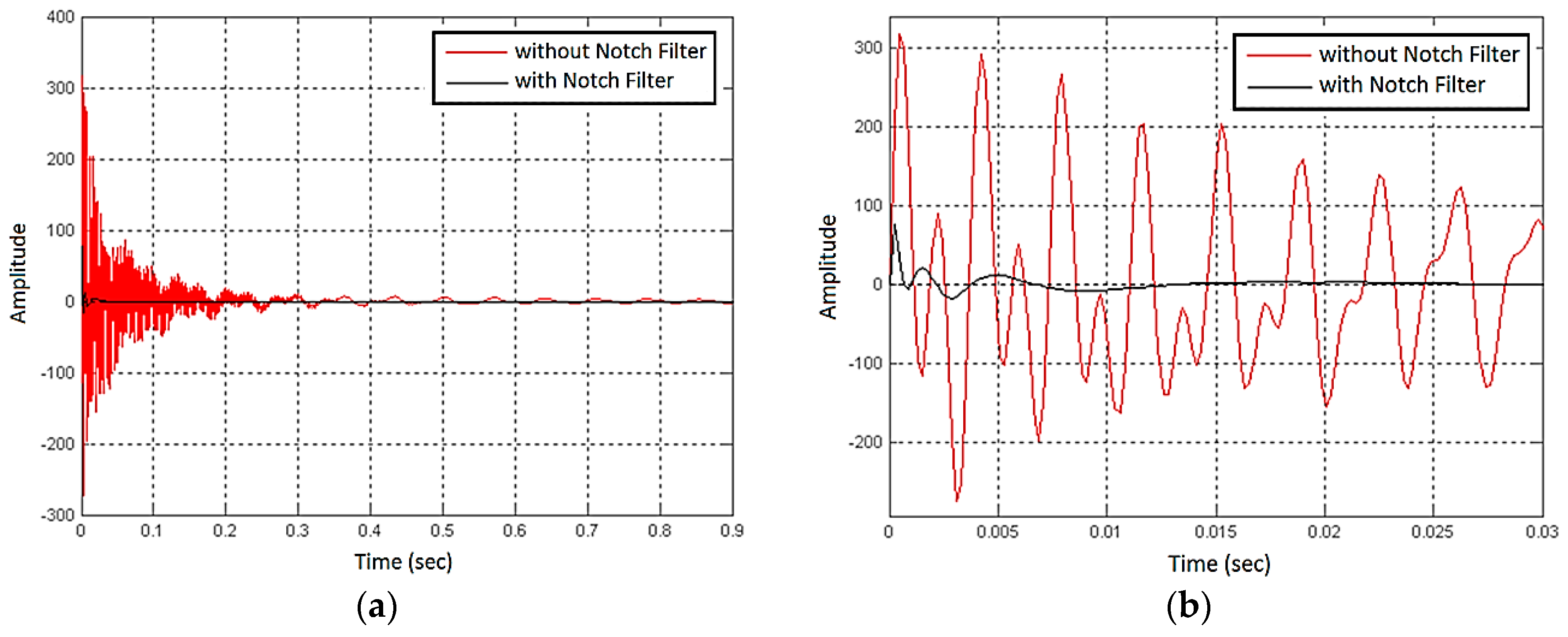
Figure 18.
Notch filter control result: (a) tracking error of step response; and (b) zoomed plot of (a).
Figure 18.
Notch filter control result: (a) tracking error of step response; and (b) zoomed plot of (a).

Figure 19.
Experimental result for the baseline structure: (a) time domain; and (b) frequency domain.
Figure 19.
Experimental result for the baseline structure: (a) time domain; and (b) frequency domain.
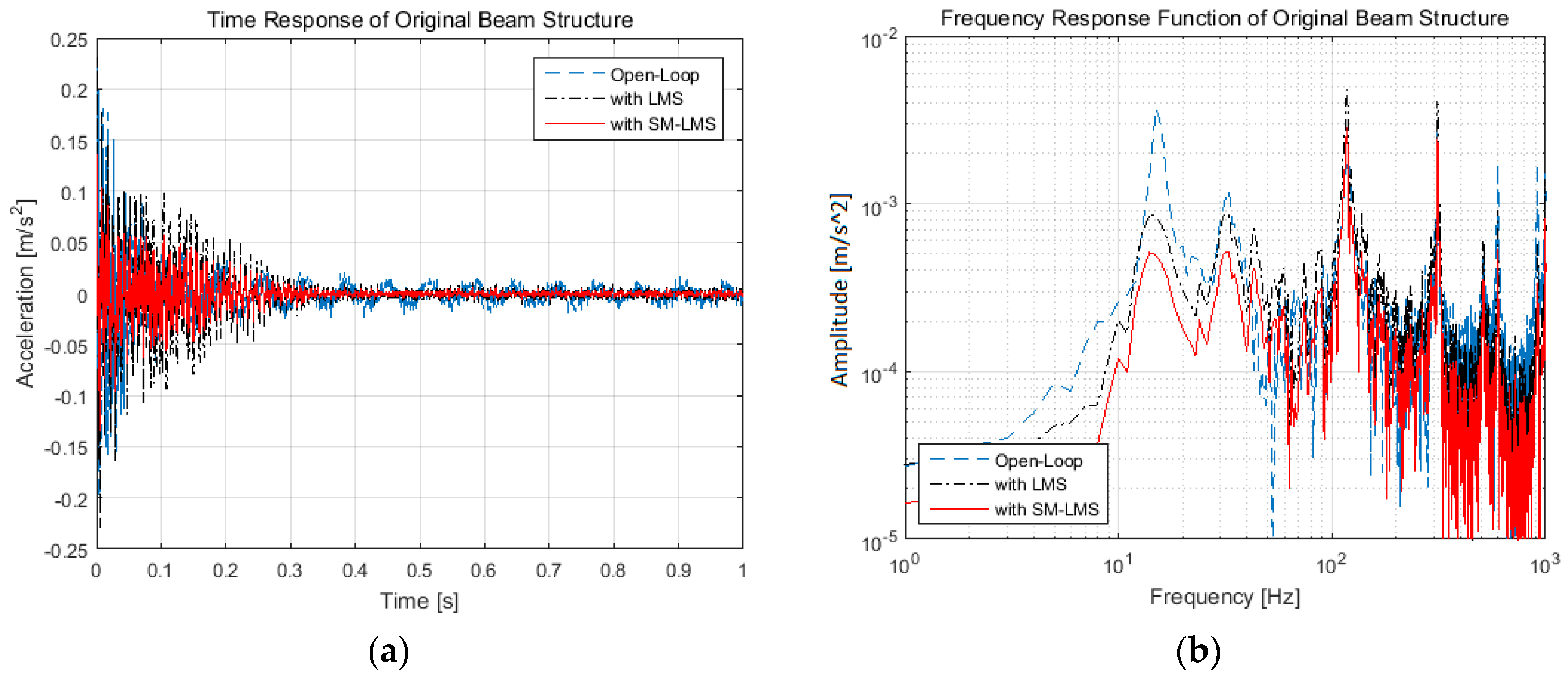
Figure 20.
Experimental result for the modified structure: (a) time domain; and (b) frequency domain.
Figure 20.
Experimental result for the modified structure: (a) time domain; and (b) frequency domain.

Table 1.
Material properties of the piezoelectric ceramic patches (PZT) patch.
| Properties | Value | Properties | Value |
|---|---|---|---|
| Thickness | 0.5 mm | Coupling Coefficient | 0.72 |
| Capacitance | 162 nF | Coupling Coefficient | 0.35 |
| Piezo. Strain Coefficient | m/V | Polarization Field | V/m |
| Piezo. Strain Coefficient | m/V | Initial Depolarization Field | V/m |
| Piezo. Voltage Coefficient | m/V | Density | 7800 kg/m3 |
| Piezo. Voltage Coefficient | m/V | Curie Temperature | 350 °C |
Table 2.
Natural frequency and damping ratio of each peak.
| Peak Number | 1 | 2 | 3 | 4 | 5 | 6 | 7 | 8 |
|---|---|---|---|---|---|---|---|---|
| Frequency (Hz) | 14.0 | 30.0 | 112.0 | 281.0 | 539.0 | 833.0 | 896.0 | 1330.0 |
| Damping Ratio | 0.0138 | 0.0222 | 0.0204 | 0.0074 | 0.0177 | 0.0058 | 0.0047 | 0.0053 |
Table 3.
Notch filter design.
| Peak | Resonance (Hz) | Damping Ratio | Notch Filter |
|---|---|---|---|
| 1 | 13.8478 | 0.7000 | |
| 2 | 28.6550 | 0.7000 | |
| 3 | 109.0439 | 0.7000 | |
| 4 | 280.1127 | 0.7000 | |
| 5 | 538.0233 | 0.7000 |
Table 4.
Vibrational amplitudes of each case for the original beam structure.
| Control | Amplitude | |||
|---|---|---|---|---|
| Peak | Open-Loop | With LMS | With SM-LMS | |
| 1st Peak (15 Hz) | 0.0037290 | 0.0008709 (12.6 dB↓) | 0.0005123 (17.2 dB↓) | |
| 2nd Peak (33 Hz) | 0.0011960 | 0.0008719 (2.7 dB↓) | 0.0005129 (7.4 dB↓) | |
| 3rd Peak (117 Hz) | 0.0017240 | 0.0048300 (8.9 dB↑) | 0.0028410 (4.3 dB↑) | |
| 4th Peak (312 Hz) | 0.0027970 | 0.0041200 (3.4 dB↑) | 0.0024240 (1.2 dB↓) | |
| Overall RMS | (0.8 dB↑) | (3.9 dB↓) | ||
Table 5.
Vibrational amplitudes of each case for the original beam structure.
| Control | Amplitude | |||
|---|---|---|---|---|
| Peak | Open-Loop | With LMS | With SM-LMS | |
| 1st Peak (15 Hz) | 0.0022920 | 0.0007087 (10.2 dB↓) | 0.0004849 (13.5 dB↓) | |
| 2nd Peak (33 Hz) | 0.0013280 | 0.0016330 (1.8 dB↑) | 0.0011170 (1.5 dB↓) | |
| 3rd Peak (117 Hz) | 0.0045400 | 0.0037110 (1.8 dB↓) | 0.0025390 (5.0 dB↓) | |
| 4th Peak (312 Hz) | 0.0028750 | 0.0046440 (4.2 dB↑) | 0.0031780 (0.9 dB↑) | |
| Overall RMS | (0.5 dB↑) | (2.8 dB↓) | ||
© 2017 by the authors. Licensee MDPI, Basel, Switzerland. This article is an open access article distributed under the terms and conditions of the Creative Commons Attribution (CC BY) license (http://creativecommons.org/licenses/by/4.0/).
Share and Cite
MDPI and ACS Style
Kim, B.; Yoon, J.-y. Enhanced Adaptive Filtering Algorithm Based on Sliding Mode Control for Active Vibration Rejection of Smart Beam Structures. Appl. Sci. 2017, 7, 750. https://doi.org/10.3390/app7070750
AMA Style
Kim B, Yoon J-y. Enhanced Adaptive Filtering Algorithm Based on Sliding Mode Control for Active Vibration Rejection of Smart Beam Structures. Applied Sciences. 2017; 7(7):750. https://doi.org/10.3390/app7070750
Chicago/Turabian StyleKim, Byeongil, and Jong-yun Yoon. 2017. "Enhanced Adaptive Filtering Algorithm Based on Sliding Mode Control for Active Vibration Rejection of Smart Beam Structures" Applied Sciences 7, no. 7: 750. https://doi.org/10.3390/app7070750
Note that from the first issue of 2016, this journal uses article numbers instead of page numbers. See further details here.