Automated Diatom Classification (Part A): Handcrafted Feature Approaches

 ,
,  ,
,  ,
,  ,
,  , and
, and
Abstract
:1. Introduction
2. Materials: Dataset Preparation
3. Valve Segmentation: Binary Thresholding
- Binary thresholding: automatic segmentation based on Otsu’s thresholding.
- Maximum area: calculation of the largest region (area).
- Hole filling: interior holes are filled if present, using mathematical morphology operators.
- Segmentation: the ROI is cropped with the coordinates of the bounding-box of the largest area (Step 2).
4. Diatom Handcrafted Feature Descriptors
4.1. Morphological Descriptors
4.1.1. Area
4.1.2. Eccentricity
4.1.3. Perimeter
4.1.4. Shape
4.1.5. Fullness
4.2. Statistical Descriptors
4.2.1. First Order Statistical: Histogram
4.2.2. Second Order Statistical: Co-Occurrence Matrix
4.3. Local Binary Patterns
4.4. Hu Moments
4.5. Texture Descriptors in the Space-Frequency Domain
Log Gabor Transform
5. Discriminant Analysis
5.1. Correlation
5.2. Sequential Forward Feature Selection
6. Classification
Bagging Trees
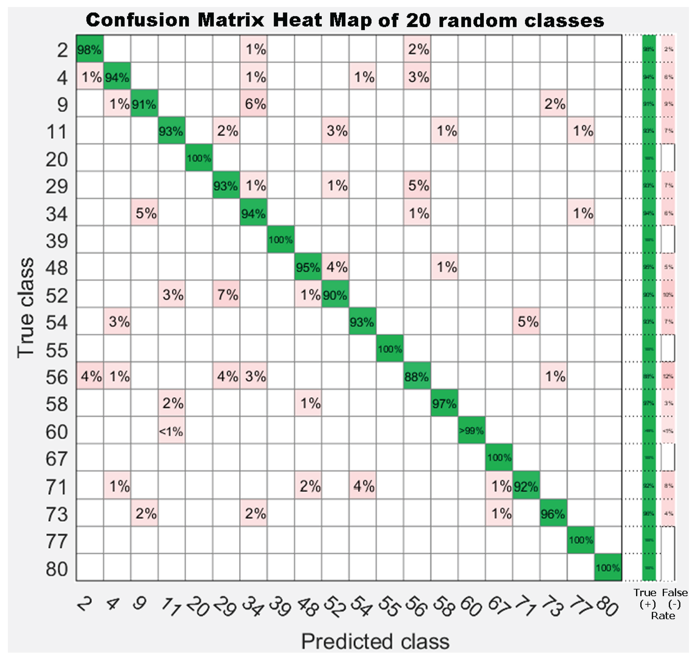
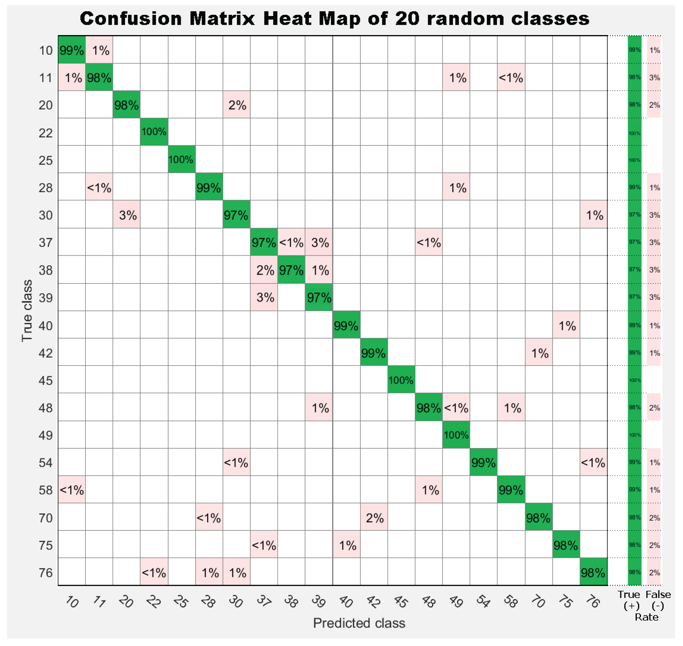
7. Results
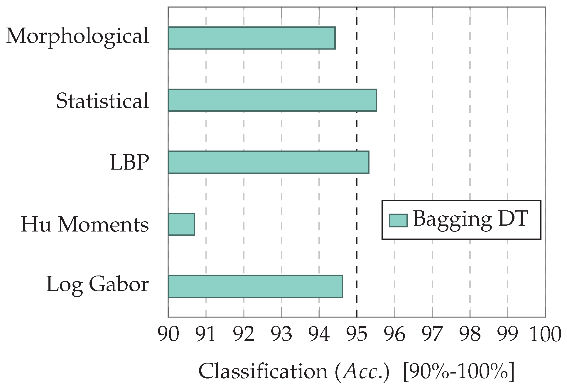
7.1. Experiment 1: Comparing Descriptor Types
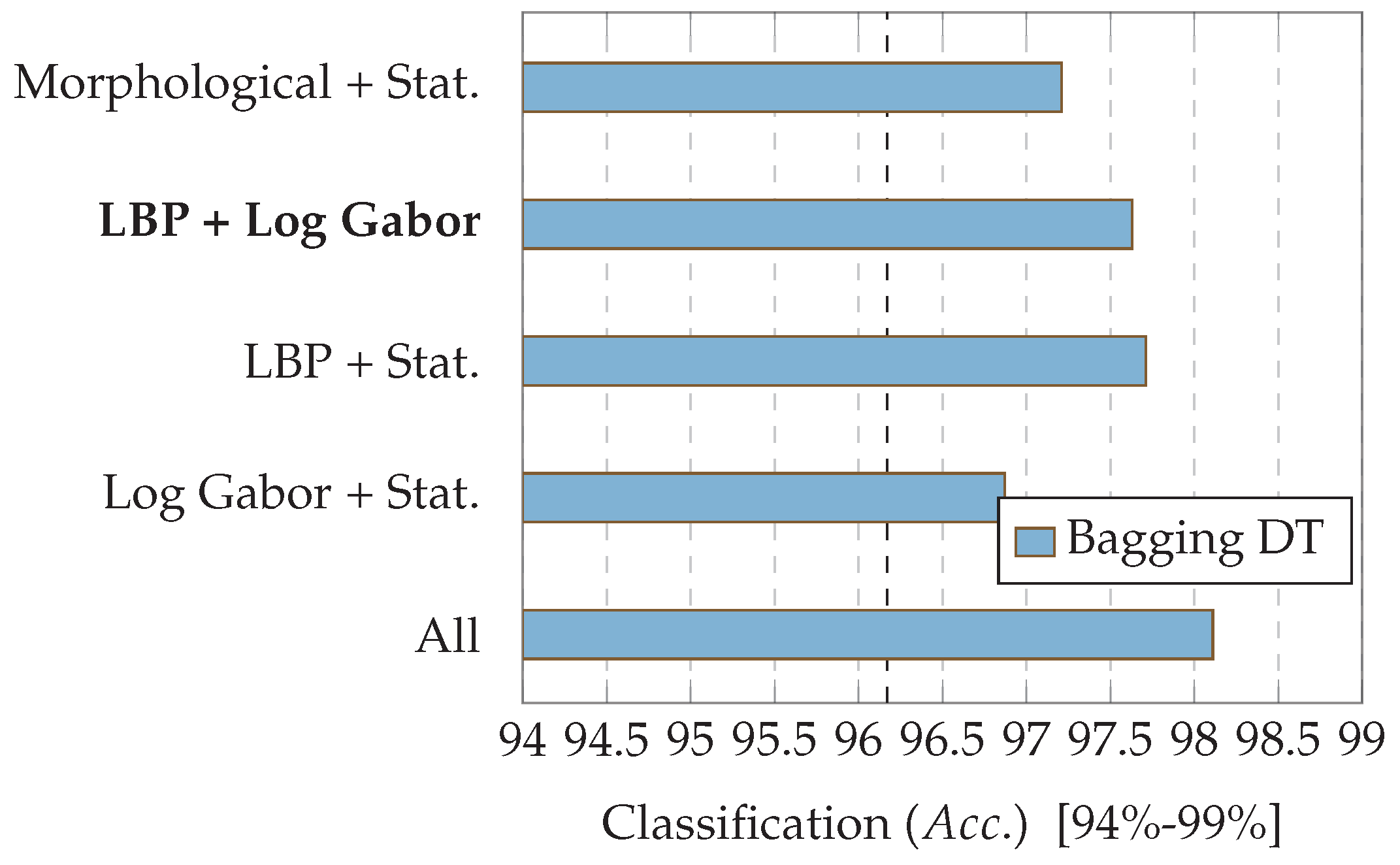
7.2. Experiment 2: Combinations of Descriptor Types
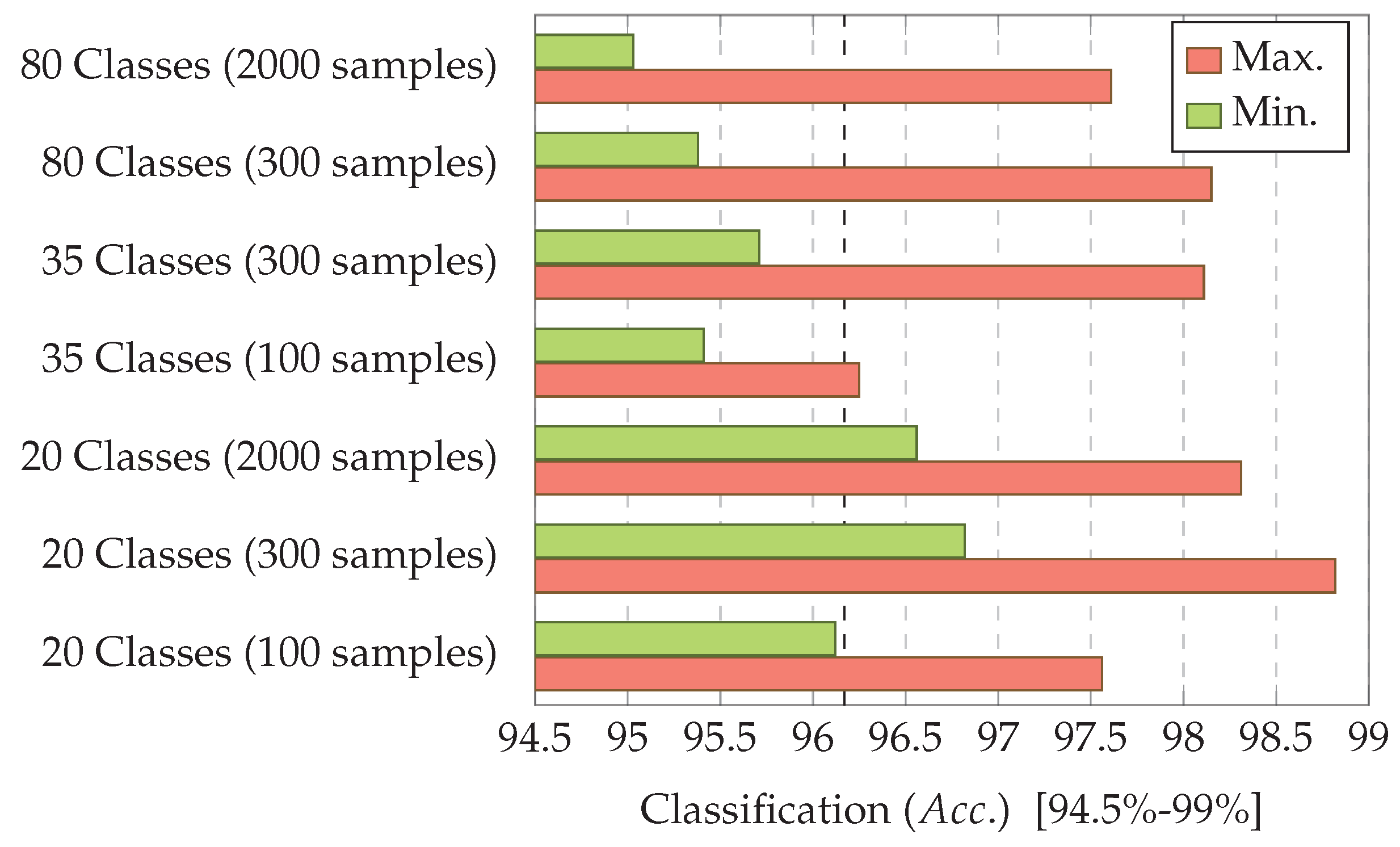
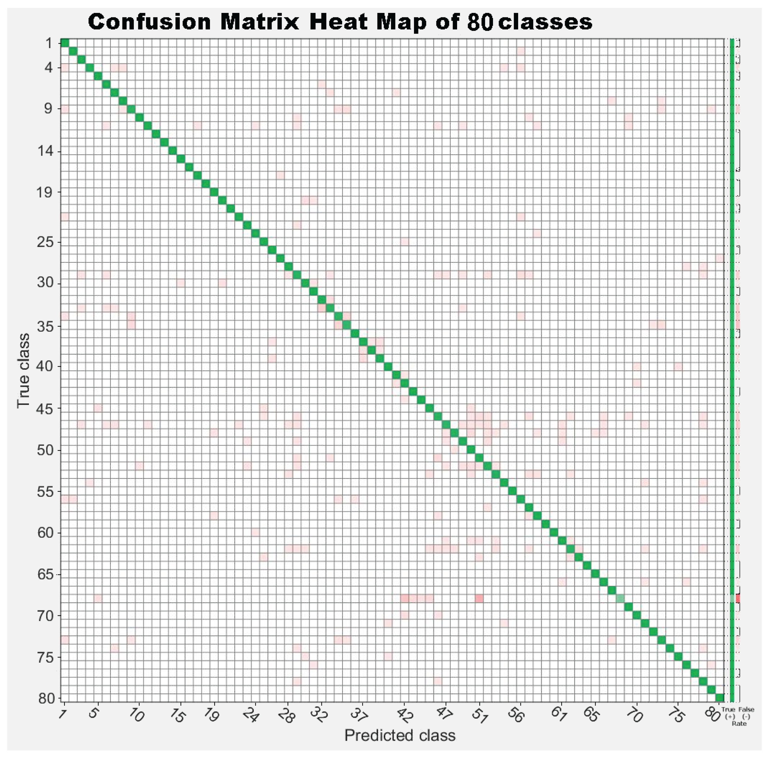
7.3. Experiment 3: Dataset Dimension
8. Conclusions
Acknowledgments
Author Contributions
Conflicts of Interest
References
- Ector, L.; Rimet, F. Using bioindicators to assess rivers in Europe: An overview. In Modelling Community Structure Infreshwater Ecosystems; Lek, S., Scardi, M., Verdonschot, P.F.M., Descy, J.-P., Park, Y.-S., Eds.; Springer: Berlin, Germany, 2005; Chapter 1; pp. 7–19. [Google Scholar]
- Wua, N.; Dong, X.; Liu, Y.; Wang, C.; Baattrup-Pedersen, A.; Riis, T. Using river microalgae as indicators for freshwater biomonitoring: Review of published research and future directions. Ecol. Indic. 2017, 81, 124–131. [Google Scholar] [CrossRef]
- Blanco, S.; Becares, E.; Cauchie, H.; Hoffmann, L.; Ector, L. Comparison of biotic indices for water quality diagnosis in the Duero Basin (Spain). Arch. Hydrobiol. Suppl. Large Rivers 2007, 17, 267–286. [Google Scholar] [CrossRef]
- Round, F.E.; Crawford, R.M.; Mann, D.G. Diatoms: Biology and Morphology of the Genera; Cambridge University Press: Cambridge, UK, 1990. [Google Scholar]
- Mann, D. The species concept in diatoms. Phycologia 1999, 38, 437–495. [Google Scholar] [CrossRef]
- John, D. Use of Algae for Monitoring Rivers III. J. Appl. Phycol. 1999, 11, 596–597. [Google Scholar] [CrossRef]
- Hicks, Y.A.; Marshall, D.; Rosin, P.; Martin, R.R.; Mann, D.; Droop, S. A model of diatom shape and texture for analysis, synthesis and identification. Mach. Vis. Appl. 2006, 17, 297–307. [Google Scholar] [CrossRef]
- Smol, J.; Stoermer, E. The Diatoms: Applications for the Environmental and Earth Sciences; Cambridge University Press: Cambridge, UK, 2010. [Google Scholar]
- European Standard, EN 14407: 2004. Water Quality—Guidance Standard for the Identification, Enumeration and Interpretation of Benthic Diatom Samples from Running Waters; Technical Report; European Commission: Brussels, Belgium, 2004. [Google Scholar]
- Wayne, R. Light and Video Microscopy, 2nd ed.; Elsevier: Amsterdam, The Netherlands, 2014. [Google Scholar]
- Desikachary, T. Electron microscope studies on diatoms. J. Microsc. 1956, 76, 9–36. [Google Scholar] [CrossRef]
- Pappas, J.; Kociolek, P.; Stoermer, E. Quantitative morphometric methods in diatom research. Nova Hedwig. Beih. 2014, 143, 281–306. [Google Scholar]
- Kloster, M.; Kauer, G.; Beszteri, B. SHERPA: An image segmentation and outline feature extraction tool for diatoms and other objects. BMC Bioinform. 2014, 15, 1. [Google Scholar] [CrossRef] [PubMed]
- Cairns, J.; Dickson, K.; Pryfogle, P.; Almeida, S.; Case, S.; Fournier, J.; Fuji, H. Determining the accuracy of coherent optical identification of diatoms. J. Am. Water Resour. Assoc. 1979, 15, 1770–1775. [Google Scholar] [CrossRef]
- Culverhouse, P.; Simpson, R.G.; Ellis, R.; Lindley, J.; Williams, R.; Parisini, T.; Reguera, B.; Bravo, I.; Zoppoli, R.; Earnshaw, G.; et al. Automatic classification of field-collected dinoflagellates by artificial neural network. Mar. Ecol. Prog. Ser. 1996, 139, 281–287. [Google Scholar] [CrossRef]
- Pech-Pacheco, J.; Alvarez-Borrego, J. Optical-digital system applied to the identification of five phytoplankton species. Mar. Biol. 1998, 132, 357–365. [Google Scholar] [CrossRef]
- Pech-Pacheco, J.; Cristobal, G.; Alvarez-Borrego, J.; Cohen, L. Automatic system for phytoplanktonic algae identification. Limnetica 2001, 20, 143–158. [Google Scholar]
- Du Buf, H.; Bayer, M. Series in Machine Perception and Artificial Intelligence. In Automatic Diatom Identification; World Scientific Publishing Co.: Singapore, 2002. [Google Scholar]
- Pappas, J.; Stoermer, E. Legendre shape descriptors and shape group determination of specimens in the Cymbella cistula species complex. Phycologia 2003, 42, 90–97. [Google Scholar] [CrossRef]
- Du Buf, H.; Bayer, M.; Droop, S.; Head, R.; Juggins, S.; Fischer, S.; Bunke, H.; Wilkinson, M.; Roerdink, J.; Pech-Pacheco, J.; et al. Diatom identification: A double challenge called ADIAC. In Proceedings of the International Conference on Image Analysis and Processing, Venice, Italy, 27–29 September 1999; pp. 734–739. [Google Scholar]
- Dimitrovski, I.; Kocev, D.; Loskovska, S.; Dzeroski, S. Hierarchical classification of diatom images using ensembles of predictive clustering trees. Ecol. Inform. 2012, 7, 19–29. [Google Scholar] [CrossRef]
- Kuang, Y. Deep Neural Network for Deep Sea Plankton Classification; Technical Report; Stanford University: Stanford, CA, USA, 2015. [Google Scholar]
- Dai, J.; Yu, Z.; Zheng, H.; Zheng, B.; Wang, N. A Hybrid Convolutional Neural Network for Plankton Classification. In Lecture Notes in Computer Science—Computer Vision, ACCV 2016 Workshops; Chen, C.-S., Lu, J., Ma, K.-K., Eds.; Springer International Publisher: Amsterdam, The Netherlands, 2017; Volume 10118, pp. 102–114. [Google Scholar]
- Pedraza, A.; Deniz, O.; Bueno, G.; Cristobal, G.; Borrego-Ramos, M.; Blanco, S. Automated Diatom Classification (Part B): A deep learning approach. Appl. Sci. 2017, 7, 460. [Google Scholar] [CrossRef]
- Lai, Q.T.; Lee, K.C.; Tang, A.H.; Wong, K.K.; So, H.K.; Tsia, K.K. High-throughput time-stretch imaging flow cytometry for multi-class classification of phytoplankton. Opt. Express 2016, 24, 28170–28184. [Google Scholar] [CrossRef] [PubMed]
- Blanco, S.; Bécares, E.; Hernández, N.; Ector, L. Evaluación de la calidad del agua en los ríos de la cuenca del Duero mediante índices diatomológicos. Publ. Téc. CEDEX Ing. Civ. 2008, 148, 139–143. [Google Scholar]
- Haralick, R.; Shanmugam, K.; Dinstein, I. Textural features for image classification. IEEE Trans. Syst. Man Cybern. 1973, SMC-3, 610–621. [Google Scholar]
- Wang, L.; He, D. Texture classification using texture spectrum. Pattern Recognit. 1990, 23, 905–910. [Google Scholar] [CrossRef]
- Ojala, T.; Pietikainen, M.; Harwood, D. Performance evaluation of texture measures with classification based on Kullback discrimination of distributions. In Proceedings of the 12th International Conference on Pattern Recognition-Conference A: Computer Vision Image Processing (IAPR), Jerusalem, Israel, 9–13 October 1994; Volume 1, pp. 582–585. [Google Scholar]
- Nava, R.; Cristobal, G.; Escalante-Ramirez, B. A comprehensive study of texture analysis based on local binary patterns. Proc. SPIE 2012, 8436, 84360E–84372E. [Google Scholar]
- Sahu, H.; Bhanodia, P. An Analysis of Texture Classification: Local Binary Patterns. J. Glob. Res. Comput. Sci. 2013, 4, 17–20. [Google Scholar]
- Ojala, T.; Pietikäinen, M.; Maenpaa, T. Multiresolution gray-scale and rotation invariant texture classification with local binary patterns. IEEE Trans. Pattern Anal. Mach. Intell. 2002, 24, 971–987. [Google Scholar] [CrossRef]
- Nava, R.; Escalante-Ramírez, B.; Cristóbal, G. Texture Image Retrieval Based on Log-Gabor Features. In Progress in Pattern Recognition, Image Analysis, Computer Vision, and Applications; Alvarez, L., Mejail, M., Gomez, L., Jacobo, J., Eds.; Lecture Notes in Computer Science; Springer: Berlin/Heidelberg, Germany, 2012; Volume 7441, pp. 414–421. [Google Scholar]
- Hu, M.K. Visual Pattern Recognition by Moment Invariants. IRE Trans. Inf. Theory 1962, IT-8, 179–187. [Google Scholar]
- Fischer, S.; Sroubek, F.; Perrinet, L.; Redondo, R.; Cristóbal, G. Self Invertible Gabor Wavelets. Int. J. Comput. Vis. 2007, 75, 231–246. [Google Scholar] [CrossRef]
- Guyon, I.; Elisseeff, A. An introduction to variable and feature selection. J. Mach. Learn. Res. 2003, 3, 1157–1182. [Google Scholar]
- Duda, R.O.; Hart, P.E.; Stork, D.G. Pattern Classification, 2nd ed.; Wiley: New York, NY, USA, 2001. [Google Scholar]
- Mitra, P.; Murthy, C.; Pal, S.K. Unsupervised feature selection using feature similarity. IEEE Trans. Pattern Anal. Mach. Intell. 2002, 24, 301–312. [Google Scholar] [CrossRef]
- Pudil, P.; Novovicova, J.; Kittler, J. Floating search methods in feature selection. Pattern Recognit. Lett. 1994, 15, 1119–1125. [Google Scholar] [CrossRef]
- Alpaydin, E. Introduction to Machine Learning, 2nd ed.; The MIT Press: Cambridge, MA, USA, 2010. [Google Scholar]
- Breiman, L. Bagging predictors. Mach. Learn. 1996, 24, 123–140. [Google Scholar] [CrossRef]


| 1. Achnanthes subhudsonis | 123 | 28. Encyonema minutum | 120 | 55. Gomphonema rhombicum | 64 |
| 2. Achnanthidium atomoides | 129 | 29. Encyonema reichardtii | 152 | 56. Humidophila contenta | 105 |
| 3. Achnanthidium caravelense | 59 | 30. Encyonema silesiacum | 108 | 57. Karayevia clevei varclevei | 84 |
| 4. Achnanthidium catenatum | 187 | 31. Encyonema ventricosum | 101 | 58. Luticola goeppertiana | 136 |
| 5. Achnanthidium druartii | 93 | 32. Encyonopsis alpina | 106 | 59. Mayamaea permitis | 40 |
| 6. Achnanthidium eutrophilum | 97 | 33. Encyonopsis minuta | 89 | 60. Melosira varians | 146 |
| 7. Achnanthidium exile | 98 | 34. Eolimna minima | 174 | 61. Navicula cryptotenella | 136 |
| 8. Achnanthidium jackii | 125 | 35. Eolimna rhombelliptica | 132 | 62. Navicula cryptotenelloides | 107 |
| 9. Achnanthidium rivulare | 305 | 36. Eolimna subminuscula | 94 | 63. Navicula gregaria | 50 |
| 10. Amphora pediculus | 117 | 37. Epithemia adnata | 72 | 64. Navicula lanceolata | 77 |
| 11. Aulacoseira subarctica | 113 | 38. Epithemia sorex | 85 | 65. Navicula tripunctata | 99 |
| 12. Cocconeis lineata | 81 | 39. Epithemia turgida | 93 | 66. Nitzschia amphibia | 124 |
| 13. Cocconeis pediculus | 49 | 40. Fragilaria arcus | 93 | 67. Nitzschia capitellata | 123 |
| 14. Cocconeis placentula var euglypta | 117 | 41. Fragilaria gracilis | 54 | 68. Nitzschia costei | 72 |
| 15. Craticula accomoda | 86 | 42. Fragilaria pararumpens | 74 | 69. Nitzschia desertorum | 71 |
| 16. Cyclostephanos dubius | 85 | 43. Fragilaria perminuta | 89 | 70. Nitzschia dissipata var media | 81 |
| 17. Cyclotella atomus | 99 | 44. Fragilaria rumpens | 49 | 71. Nitzschia fossilis | 76 |
| 18. Cyclotella meneghiniana | 103 | 45. Fragilaria vaucheriae | 82 | 72. Nitzschia frustulum var frustulum | 226 |
| 19. Cymbella excisa var angusta | 79 | 46. Gomphonema angustatum | 86 | 73. Nitzschia inconspicua | 255 |
| 20. Cymbella excisa var excisa | 241 | 47. Gomphonema angustivalva | 55 | 74. Nitzschia tropica | 65 |
| 21. Cymbella excisiformis var excisiformis | 142 | 48. Gomphonema insigniforme | 90 | 75. Nitzschia umbonata | 91 |
| 22. Cymbella parva | 177 | 49. Gomphonema micropumilum | 89 | 76. Rhoicosphenia abbreviata | 94 |
| 23. Denticula tenuis | 181 | 50. Gomphonema micropus | 117 | 77. Skeletonema potamos | 155 |
| 24. Diatoma mesodon | 115 | 51. Gomphonema minusculum | 158 | 78. Staurosira binodis | 94 |
| 25. Diatoma moniliformis | 134 | 52. Gomphonema minutum | 93 | 79. Staurosira venter | 87 |
| 26. Diatoma vulgaris | 88 | 53. Gomphonema parvulum saprophilum | 52 | 80. Thalassiosira pseudonana | 70 |
| 27. Discostella pseudostelligera | 82 | 54. Gomphonema pumilum var elegans | 128 |
| CATEGORY | HANDCRAFTED FEATURE | TOTAL |
|---|---|---|
| Morphological | Area, eccentricity (3 eccentricities) | 7 features |
| Perimeter, shape, fullness | ||
| Statistical | 1st order (histogram) | 13 features |
| 2nd order (co-occurrence matrix) | 19 features | |
| pixels | ||
| , , , | ||
| Texture space | LBP | Stat.241 features |
| Moments | Hu | 7 moments |
| Space-frequency | Log Gabor | 4 scales (6 orientations) |
| 241 × 4 = 964 features |
| Mean | |
| Mode | |
| Minimum | |
| Maximum | |
| Variance | |
| Range | |
| Entropy | |
| 1st Quartile | |
| 2nd Quartile | |
| 3rd Quartile | |
| Interquartile Range | |
| Asymmetry | |
| Kurtosis |
| Energy | |
| Variance | |
| Contrast | , |
| Dissimilarity | |
| Correlation | |
| Autocorrelation | |
| Entropy | |
| Measure of Correlation 1 | |
| Measure of Correlation 2 | |
| Cluster Shade | |
| Cluster Prominence | |
| Maximum Probability | , , |
| Sum Average | |
| Sum Entropy | |
| Sum Variance | |
| Difference Entropy | |
| Difference Variance | |
| Homogeneity 1 | |
| Homogeneity 2 | |
| H bins number, and entropy of and . | |
| ; | |
| ; | |
| ; | |
| ; , | |
| ; , | |
| 1 | M | Shape | 35 | LBP | Contrast (d = 3, ) | 69 | G1 | Contrast (d = 1, ) |
| 2 | S | 1st Quartile | 36 | G4 | Correlation 1 (d = 1, ) | 70 | S | ΣAverage (d = 1, ) |
| 3 | M | Asymmetry | 37 | G4 | Correlation 1 (d = 1, ) | 71 | G4 | Entropy |
| 4 | S | Contrast (d = 1, ) | 38 | S | Energy (d = 1, ) | 72 | LBP | Cluster Prominence (d = 1, ) |
| 5 | S | Energy | 39 | S | Correlation 1 (d = 3, ) | 73 | G4 | Cluster Shade (d = 1, ) |
| 6 | S | Contrast (d = 1, ) | 40 | S | Homogeneity 1 (d = 1, ) | 74 | LBP | Correlation 1 (d = 3, ) |
| 7 | G4 | Correlation 1 (d = 3, ) | 41 | S | Correlation 1 (d = 3, ) | 75 | S | Entropy |
| 8 | S | Interquartile Range | 42 | LBP | ΔVariance (d = 1, ) | 76 | G3 | ΔEntropy (d = 1, ) |
| 9 | G4 | ΔEntropy (d = 1, ) | 43 | G3 | Correlation 1 (d = 3, ) | 77 | LBP | Correlation (d = 1, ) |
| 10 | LBP | 1st Quartile | 44 | G2 | Contrast (d = 1, ) | 78 | LBP | Contrast (d = 1, ) |
| 11 | LBP | Correlation 1 (d = 3, ) | 45 | LBP | Correlation 1 (d = 3, ) | 79 | G3 | Energy (d = 1, ) |
| 12 | LBP | Max. Probability (d = 1, ) | 46 | LBP | Correlation 1 (d = 3, ) | 80 | G4 | Correlation 1 (d = 5, ) |
| 13 | LBP | Contrast (d = 3, ) | 47 | LBP | Max. Probability (d = 1, ) | 81 | LBP | Homogeneity 1 (d = 1, ) |
| 14 | S | Variance | 48 | S | Correlation 1 (d = 5, ) | 82 | G4 | ΔVariance (d = 1, ) |
| 15 | LBP | Correlation 1 (d = 1, ) | 49 | G4 | ΔVariance (d = 1, ) | 83 | LBP | Max. Probability (d = 3, ) |
| 16 | S | Kurtosis | 50 | S | 3rd Quartile | 84 | G4 | Entropy (d = 1, ) |
| 17 | LBP | Autocorrelation (d = 3, ) | 51 | S | Correlation 1 (d = 5, ) | 85 | G4 | Correlation 1 (d = 1, ) |
| 18 | G4 | ΔEntropy (d = 3, ) | 52 | S | Dissimilarity (d = 5, ) | 86 | G3 | ΔVariance (d = 1, ) |
| 19 | S | Autocorrelation (d = 1, ) | 53 | S | Max. Probability (d = 1, ) | 87 | G4 | Correlation (d = 1, ) |
| 20 | G4 | Dissimilarity (d = 1, ) | 54 | S | Homogeneity 1 (d = 1, ) | 88 | LBP | Correlation 1 (d = 3, ) |
| 21 | G3 | ΔEntropy (d = 1, ) | 55 | S | Correlation (d = 1, ) | 89 | G3 | Correlation 1 (d = 1, ) |
| 22 | LBP | Contrast (d = 1, ) | 56 | G4 | Correlation 1 (d = 3, ) | 90 | G3 | Contrast (d = 1, ) |
| 23 | LBP | Contrast (d = 5, ) | 57 | S | Correlation 1 (d = 3, ) | 91 | G4 | Cluster Prominence (d = 1, ) |
| 24 | LBP | Contrast (d = 3, ) | 58 | LBP | Contrast (d = 5, ) | 92 | G3 | Correlation (d = 1, ) |
| 25 | S | Sum Average (d = 1, ) | 59 | LBP | Correlation 1 (d = 5, ) | 93 | G4 | Contrast (d = 1, ) |
| 26 | LBP | Contrast (d = 5, ) | 60 | G4 | Correlation 1 (d = 5, ) | 94 | M | Area |
| 27 | G4 | Correlation 1 (d = 1, ) | 61 | LBP | Correlation 1 (d = 1, ) | 95 | G3 | Cluster Shade (d = 1, ) |
| 28 | G4 | Dissimilarity (d = 1, ) | 62 | S | Correlation1 (d = 1, ) | 96 | G2 | Dissimilarity (d = 1, ) |
| 29 | S | Homogeneity 1 (d = 1, ) | 63 | LBP | Homogeneity 1 (d = 3, ) | 97 | G3 | Correlation 1 (d = 3, ) |
| 30 | G4 | Kurtosis | 64 | LBP | Homogeneity 1 (d = 3, ) | 98 | M | Eccentricity |
| 31 | G4 | Dissimilarity (d = 1, ) | 65 | G3 | Correlation (d = 1, ) | 99 | LBP | Max. Probability (d = 3, ) |
| 32 | G4 | Energy (d = 1, ) | 66 | G3 | Correlation 1 (d = 1, ) | 100 | LBP | Correlation 1 (d = 1, ) |
| 33 | LBP | Homogeneity 1 (d = 1, ) | 67 | G3 | Kurtosis | |||
| 34 | G3 | Dissimilarity (d = 1, ) | 68 | S | 2nd Quartile |
© 2017 by the authors. Licensee MDPI, Basel, Switzerland. This article is an open access article distributed under the terms and conditions of the Creative Commons Attribution (CC BY) license (http://creativecommons.org/licenses/by/4.0/).
Share and Cite
Bueno, G.; Deniz, O.; Pedraza, A.; Ruiz-Santaquiteria, J.; Salido, J.; Cristóbal, G.; Borrego-Ramos, M.; Blanco, S. Automated Diatom Classification (Part A): Handcrafted Feature Approaches. Appl. Sci. 2017, 7, 753. https://doi.org/10.3390/app7080753
Bueno G, Deniz O, Pedraza A, Ruiz-Santaquiteria J, Salido J, Cristóbal G, Borrego-Ramos M, Blanco S. Automated Diatom Classification (Part A): Handcrafted Feature Approaches. Applied Sciences. 2017; 7(8):753. https://doi.org/10.3390/app7080753
Chicago/Turabian StyleBueno, Gloria, Oscar Deniz, Anibal Pedraza, Jesús Ruiz-Santaquiteria, Jesús Salido, Gabriel Cristóbal, María Borrego-Ramos, and Saúl Blanco. 2017. "Automated Diatom Classification (Part A): Handcrafted Feature Approaches" Applied Sciences 7, no. 8: 753. https://doi.org/10.3390/app7080753