The Synchrosqueezing Algorithm Based on Generalized S-transform for High-Precision Time-Frequency Analysis


Geomathematics Key Laboratory of Sichuan Province, Chengdu University of Technology, Chengdu 610059, China
*
Author to whom correspondence should be addressed.
Appl. Sci. 2017, 7(8), 769; https://doi.org/10.3390/app7080769
Submission received: 4 July 2017
/
Revised: 23 July 2017
/
Accepted: 26 July 2017
/
Published: 28 July 2017
Abstract
:In this paper, a new time-frequency analysis method—Synchrosqueezing Generalized S-transform (SSGST)—is proposed to meet the needs of high-resolution seismic signal processing and interpretation. The basic wavelet of the generalized S-transform (GST) in the paper is a modulated harmonic wave with four undetermined parameters that can be constructed by adjusting the four parameters to make the GST more suitable for seismic signals processing. The SSGST method squeezes and reconstructs the complex coefficient spectra of GST results along the frequency direction so that the energy distributions on the time-frequency spectra are concentrated around the real instantaneous frequency of the signal; thus, the time-frequency resolution can be improved. Based on mathematical theory, the basic principle of the new transformation method is given, and the mathematical expressions of the positive transformation and lossless inverse transformation of the method are strictly deduced. The experimental results of numerical signals illustrate that the proposed method can correctly decompose signals with different spectral characteristics into a high time-frequency resolution spectrum and can recovery the original signal from the time-frequency spectrum with satisfying reconstructing accuracy. Application on field seismic data shows the superiority of the new method in seismic time-frequency analysis for hydrocarbon detection.
1. Introduction
Time-frequency analysis, a powerful tool for seismic data analysis, plays a significant role in oil and gas exploration and development. It maps a 1D signal in the time domain into a 2D time-frequency spectrum, which can effectively reveal important details of seismic data and provide valuable information for reservoir characterization.
The commonly used methods for seismic time-frequency analysis include short-time Fourier transform (STFT), wavelet transform (WT), and S-transform (ST). STFT suffers from a fixed time-frequency resolution caused by a preselecting window length. To overcome this disadvantage, wavelet-based methods have been adopting and show obvious superiority in spectral resolution (e.g., [1]). Although WT leads to a more flexible trade-off between frequency and time resolution due to the variable length of the mother wavelet, it still displays spectral smearing due to the finite size of the operator. The S-transform (ST) proposed by Stockwell et al. [2] can be interpreted as a special case of the Continuous Wavelet Transform (CWT) based on Morlet wavelet, but with minor phase and amplitude adjustments.. It eliminates the limitation of fixed window length in STFT and also has the multi-resolution ability of WT. In other words, ST can effectively avoid the existing deficiencies of the above two methods [3]. Nevertheless, the fixed changing trend of the basic wavelet in ST limits its practical application. Therefore, many researchers have proposed a variety of forms of generalized S transform (GST) on the basis of ST by introducing variable window parameters to improve the flexibility and adaptability of the wavelet window [4,5,6,7,8,9]. The method based on Empirical Mode Decomposition (EMD) [10] or its extended algorithms (e.g., ensemble empirical mode decomposition (EEMD), complete ensemble empirical mode decomposition (CEEMD)) are other time-frequency transforms, which have also been applied in seismic data and have achieved excellent time-frequency resolution (e.g., [11,12,13,14]). Although EMD-based methods are useful for many applications, there is still a lack of mathematical foundation and a high computational cost.
Synchrosqueezing transform (SST) is a relatively new technique based on the combination of time-frequency methods followed by a reassignment step [15,16] that can be also regarded as an alternative to the EMD method considering their similar time-frequency resolution. SST can improve the energy concentration of time-frequency representation by applying a post-processing reallocation to the original representation. At each time or space location, the SST reassigns values of the initial representation based on their local oscillation. However, differing from EMD, the transformation process of SST is generated by strict mathematical derivation, which is beneficial to the understanding of the method and can be improved according to the specific application. At present, the synchrosqueezing algorithm has been extended to time-frequency representations based on the STFT [17,18,19], the wave packet transform [20], the curvelet transform [21], the ST [22], or the CWT [23,24], which is used in the synthetic examples of this paper. SST was originally applied to the audio signal analysis. Subsequently, many efforts have been made to use this method for seismic data processing and interpretation. In 2014, Herrera et al. [25] identified channels from seismic data using SST successfully and highlighted the advantages of this method over EMD and EEMD. In 2015, they also used SST to separate the P and S waves of microseismic data [26]. Later, Mousavi et al. (2016) [27] used it for microseismic detection. Mousavi and Langston (2017) [28] showed that SST can be used to improve the denoising of seismic data. Tary et al. (2017) [15,29] used it for attenuation estimation.
The generalized S-transform (GST) introduced by Gao et al. [6] overcomes the dilemma of the fixed wavelet in ST by introducing four undetermined parameters (amplitude, energy decay rate, energy delay time, and video rate) to construct the basic wavelet adaptive to the non-stationary signal characteristics in practical application. Due to having no restriction of the time window length, GST can obtain real time-frequency spectra with excellent time-frequency resolution, which provides more possibility and higher accuracy for the detailed information extraction of complicated non-stationary signals than ST. Since seismic signals are non-stationary and non-linear and show the characteristics of broadband and multi-frequency, using the GST instead of ST for seismic time-frequency analysis has been proven to be advisable.
In this paper, inspired by the theory of SST and the advantages of the GST over ST, we propose a novel time-frequency analysis method that we have named synchrosqueezing generalized S-transform (SSGST). The rest of this paper is organized as follows: Section 2 gives a brief review of GST and SST and then deduces the mathematical formulas of the newly proposed method in detail. In Section 3, three synthetic examples are employed to explore the performance of the SSGST method. Section 4 illustrates the effectiveness of the proposed method in the field seismic data analysis for hydrocarbon detections. Conclusions are drawn in Section 5.
2. Principles
2.1. Generalized S-transform (GST) with Four Parameters
Standard S-transform (ST) is proposed by Stockwell et al. [2]. This transform is defined as,
The basic wavelet function in standard ST is,
where represents a signal, denotes the ST of . is frequency, is time and denotes the time shift.
The inverse transform of the standard ST is obtained by,
Although ST inherits the advantages of STFT and WT, its application is limited because of its fixed basic wavelet function. Gao et al. use a modulated harmonic wave with four undetermined parameters to replace the basic wavelet in ST to overcome the disadvantage caused by the fixed basic wavelet function. The modulated harmonic wave is written as,
where is amplitude of the basic wavelet, is energy attenuation ratio , is energy delay time and is video frequency of the basic wavelet.
So the generalized S-transform (GST) with four parameters of a signal is,
where denotes the result of the GST with four parameters. Its inverse transform is,
where represents the inverse transform of Fourier transform.
It is obvious that the four-parameter GST is degenerated into a standard ST when , , and .
2.2. Synchrosqueezing Transform (SST)
SST is a new reassignment technique and a powerful tool for precisely decomposing and analyzing a signal. It can provide a sharpened time-frequency representation by applying a post-processing reallocation to the original representation. Thus, the SST algorithm can be divided into two step: (1) computing the instantaneous frequency using the original time-frequency coefficients and (2) squeezing and reassigning step. So far, many researchers have developed SST algorithms combining a reassignment step and different time-frequency decomposing methods such as continuous wavelet transform, short-time Fourier transform, curvelet tranform, S-transform, and wavelet packet transform.
Among these algorithms, synchrosqueezing continuous wavelet transform (SSCWT) is used for comparison with the new method proposed in this paper. It was proposed by Daubechies et al. [24] and can obtain higher resolution time-frequency spectra by squeezing and reconstructing the values of continuous wavelet transform (CWT) in the frequency direction. Thus, taking this method as an example, we briefly introduce the principle of SST.
First, we calculate the CWT of a signal as,
where denotes the continuous wavelet transform of a signal . is the scale factor, and is the time translation factor. is a mother wavelet and is the complex conjugate of .
Then, the instantaneous frequency at any time-scale location is,
Secondly, we reassign values of the time-frequency representation based on its local oscillation. The result of SST is,
where is the scale value and . denotes the frequency point. The Equation (9) means that the CWT spectra values between are squeezed to the frequency point along the frequency direction. Thus, the time-frequency resolution becomes better.
The inverse transform of SST is written as
In Equation (10), , is the complex conjugate of the Fourier transform of the mother wavelet .
2.3. Synchrosqueezing Generalized S-transform (SSGST)
In this part, we give the basic principle of SSGST and derive the mathematical expressions of the positive transformation and lossless inverse transformation based on the mathematical theory.
First, the Equation (5) can be reformulated as,
Let , then Equation (11) is expressed as,
where, represents the complex conjugate of .
According to the Parseval theorem and transformation properties of scale and translation in Fourier Transform, the Equation (13) can be derived as follows:
where, denotes the Fourier Transform result of the signal . is the complex conjugate of the Fourier Transform result of . Especially, if , .
Then, we can calculate the instantaneous frequency of the signal by using Equation (14):
Now, we testify the feasibility and rationality of Equation (14) using an example of a harmonic wave . The Fourier transform result of the signal is given as,
where and denote, respectively, the amplitude and frequency of the harmonic wave .
The GST of the harmonic wave can be calculated by substituting Equation (15) into Equation (13) and is given as,
According to Equation (14), the instantaneous frequency of the harmonic signal is,
Therefore, the instantaneous frequency can be estimated by Equation (14). SSGST is defined as the Equation (18) according to the theories of synchrosqueezing.
where, is the frequency of the SSGST result. is the half length of frequency range centered on the frequency point . denotes the discrete frequency points in frequency ranges of the GST, and .
The Equation (18) represents that the time-frequency spectra values among the frequency range are superimposed on the frequency point , so that the SSGST has higher accuracy of time-frequency decomposition ability.
Next, the inverse transform of SSGST is derived as follows:
We integrate over frequency on both sides of Equation (13), and obtain the Equation (19) by replacing with .
Let , (19) can be rewritten as,
Because the signal is the real signal, we extract the real component from the Equation (20) as the following reconstructed signal:
Through discretizing the equation on the right-hand side of Equation (21) and combining Equation (18), the inverse transform of SSGST is given as,
Therefore, we can recover the original signal from the SSGST spectrum by using the Equation (22).
3. Synthetic Examples
In this section, to clarify the superiority of the proposed SSGST method, two signals that are commonly used for testing the performance of time-frequency distribution have been adopt. We also designed a synthetic signal to further illustrate the effectiveness of the proposed method for separating different frequency components from complicated signals and signal reconstruction. In processing numerical signals, comparisons are made between SSGST and the other time-frequency methods, such as CWT, GST, and SSCWT.
3.1. The Double Linear Chirped Signal
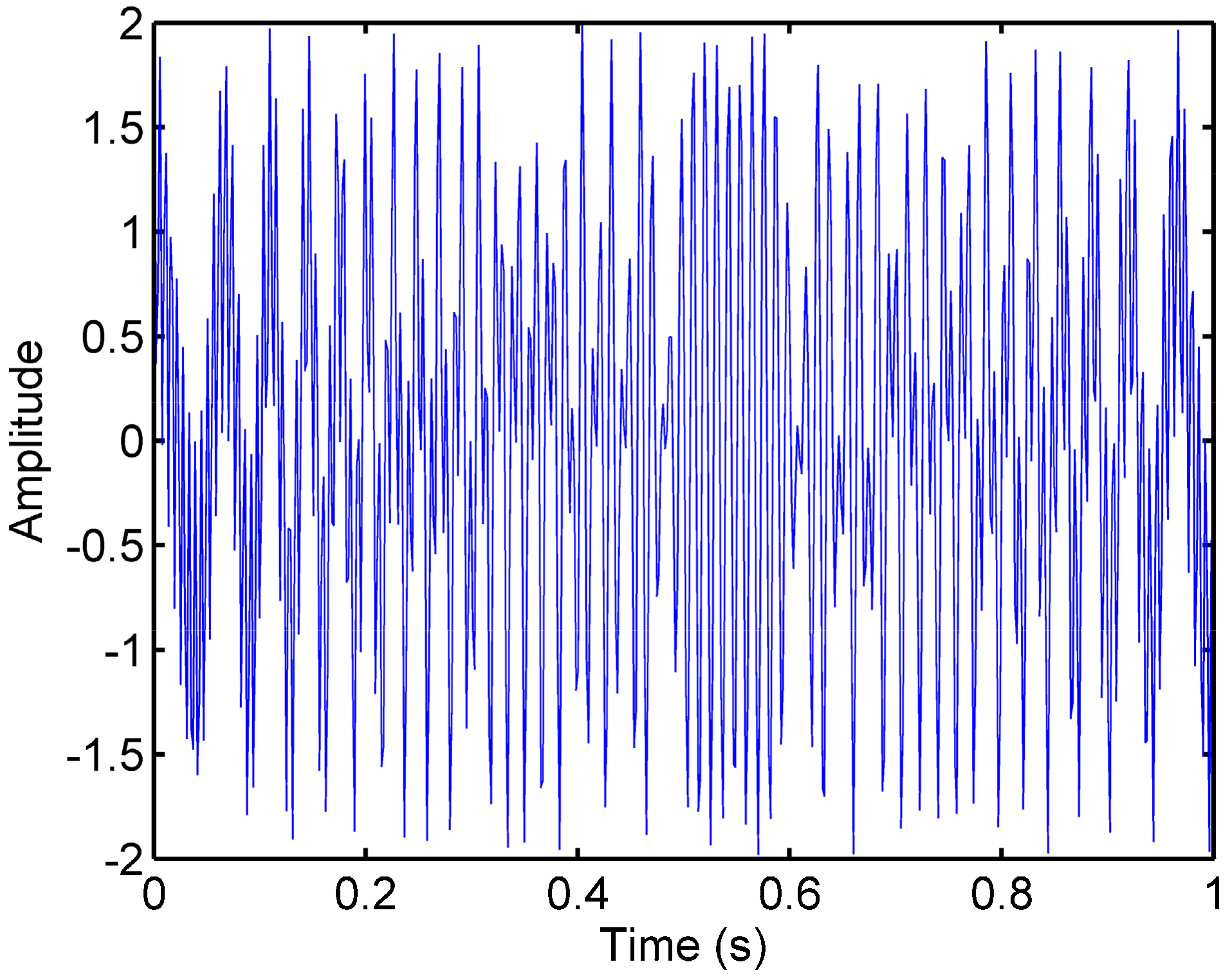
Linear frequency-modulated (FM) signal is a generally accepted model that is used to test the performance of time-frequency distribution. The double linear chirped signal shown in Figure 1 is composed of two crossing linear chirps whose main frequencies are linearly increasing and decreasing with time, respectively.
The CWT, GST, SSCWT, and SSGST methods are applied to this signal, and the relative results analysis are shown in Figure 2. As can be seen, although all energy centers around the true instantaneous frequencies of the signal, the energy of the CWT and GST results smears heavily (Figure 2a,b). In contrast, due to the effect of the “squeezing,” SSCWT and SSGST squeeze all time-frequency coefficients into the time-frequency trajectory, which makes the spectra more energy-concentrated, as displayed in Figure 2c,d. In other words, SSCWT and SSGST show higher time-frequency resolution than CWT and GST. Furthermore, compared with the result of SSCWT, SSGST shows that the signal energy is much more concentrated around the ridge and that the time-frequency resolution performs better. The arrows show that there is no distinct “steps” in the SSGST result compared with the result of SSCWT.
3.2. The Double Hyperbolic Chirped Signal
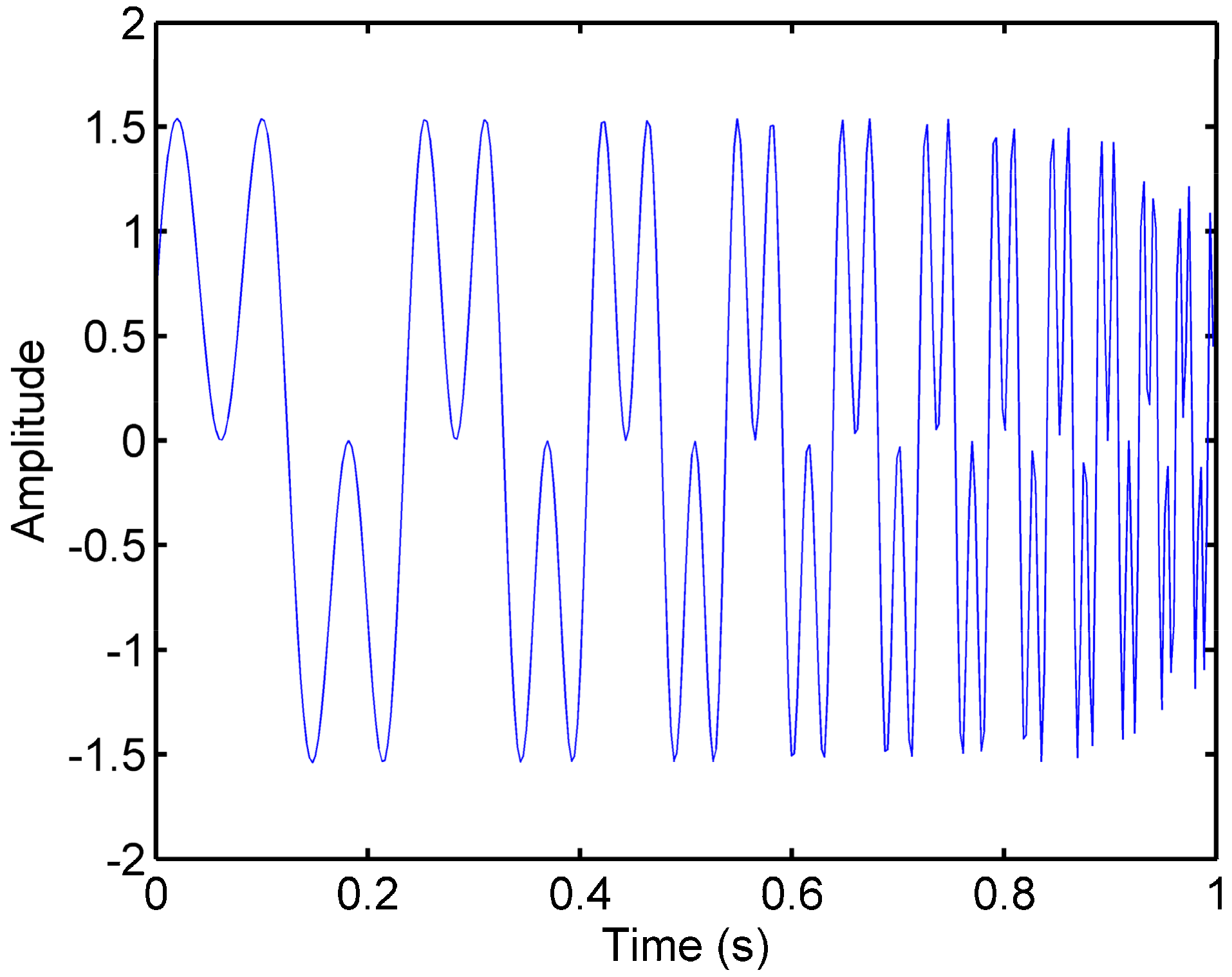
In order to futher verify the effectiveness of the SSGST method in dealing with non-stationary signal whose time-frequency characteristics is more complicated, we apply it to the double hyperbolic chirped signal (Figure 3), whose main frequency hyperbolic increases.
The results generated by the CWT, GST, SSCWT, and SSGST methods are shown in Figure 4. The time-frequency represents in Figure 4a,b resulted from the CWT and GST show poor energy concentration. However, as can be seen from Figure 4c,d, both SSCWT and SSGST provide higher resolution time-frequency result than CWT and GST, and they are good approximations of the signal’s instantaneous frequency. Compared with the SSCWT result, the SSGST representation shows an obviously higher energy concentration (see Figure 4c,d).
According to the comparison of the SSGST method with the CWT, GST, and SSCWT methods, we find that the SSGST method has better performance in improving time-frequency resolution and accuracy of time-frequency resolution. Moreover, there is no spurious frequency in the time-frequency spectrum of SSGST; thus, high-resolution time-frequency analysis results can be obtained accurately by the SSGST method.
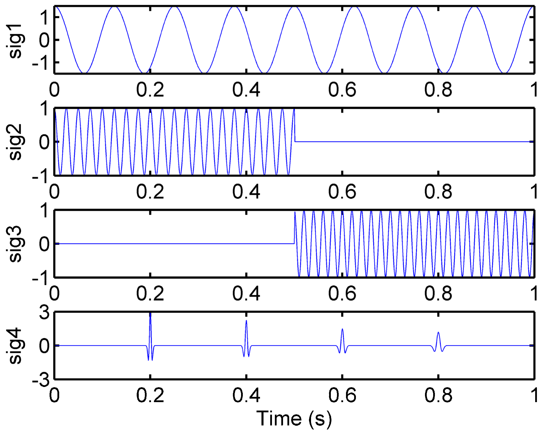
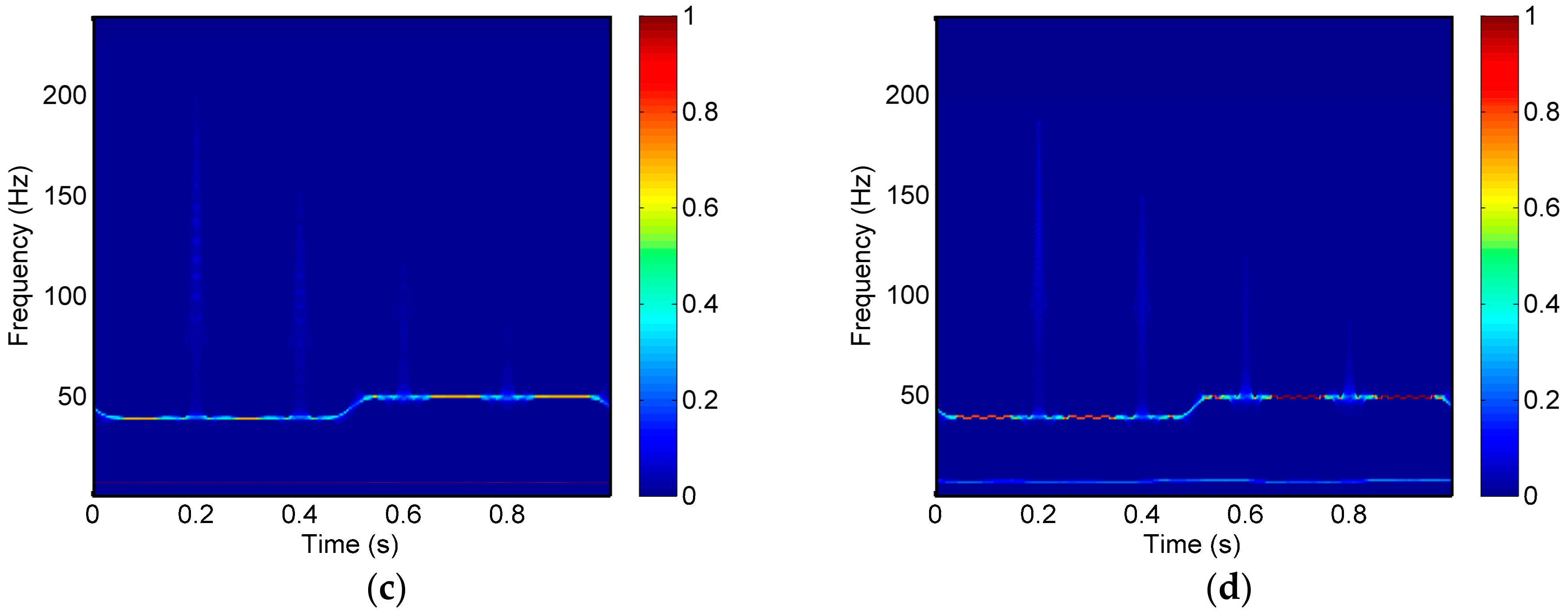
3.3. A Synthetic Seismic Signal
Next, we apply CWT GST, SSCWT, and SSGST to a synthetic seismic signal for illustrating the effectiveness of separating the different frequency components of seismic signals. The synthetic signal is comprised of a cosinusoid signal , two intermittent signal and , and a simulated attenuate seismic signal , which is composed of four different frequency Ricker wavelets at 0.2 s, 0.4 s, 0.6 s, and 0.8 s of 100 Hz, 80 Hz, 65 Hz, and 55 Hz, respectively (Figure 5).
The results of the synthetic signal obtained by CWT, GST, SSCWT, and SSGST are presented in Figure 6. As can be seen in Figure 6, all methods can separate the frequency components well, and the time-frequency representation generated by the SSCWT and SSGST methods provide clearer time-frequency resolution than the CWT and GST methods. Comparing Figure 6b with Figure 6d, SSGST and SSCWT show similar frequency resolution. However, SSGST can depict the 8Hz cosine signal with higher resolution than SSCWT.
3.4. Comparative Quantification and Reconstruction Analysis
To quantify the performance of the SSGST and the other algorithms for generating TF representations of synthetic examples, we choose Rényi Entroy [30] as a quantitative performance index. The Rényi entropy is an objective indicator to evaluate the energy concentration of a time-frequency result; a lower Rényi entropy value denotes a more energy-concentrated time-frequency representation. The corresponding Rényi entropies are listed in Table 1. As can be seen in Table 1, in terms of the first and second synthetic examples, the SSGST result has the lowest Rényi entropy compared with the other time-frequency transforms. In the synthetic seismic signal processing, the Rényi entropy of the SSGST result ranks behind only the SSCWT. Therefore, in summary, compared with the other methods mentioned above, the SSGST method is more likely to obtain an energy-concentrated time-frequency result.
We adopted the mean square error (MSE) to validate the reconstruction ability of the SSGST method. The corresponding MSE of the SSGST and the other algorithms are listed in Table 2. As shown in Table 2, the MSE values of SSGST are in the range of acceptable reconstruction error while taking the MSE values of other time frequency transforms as references.
Therefore, the SSGST method improves the resolution of time-frequency and also has a good reflection of strong or weak amplitude and high or low frequency. The newly proposed method can also reconstruct the original signal well with a lower reconstruction error.
4. Field Data Examples
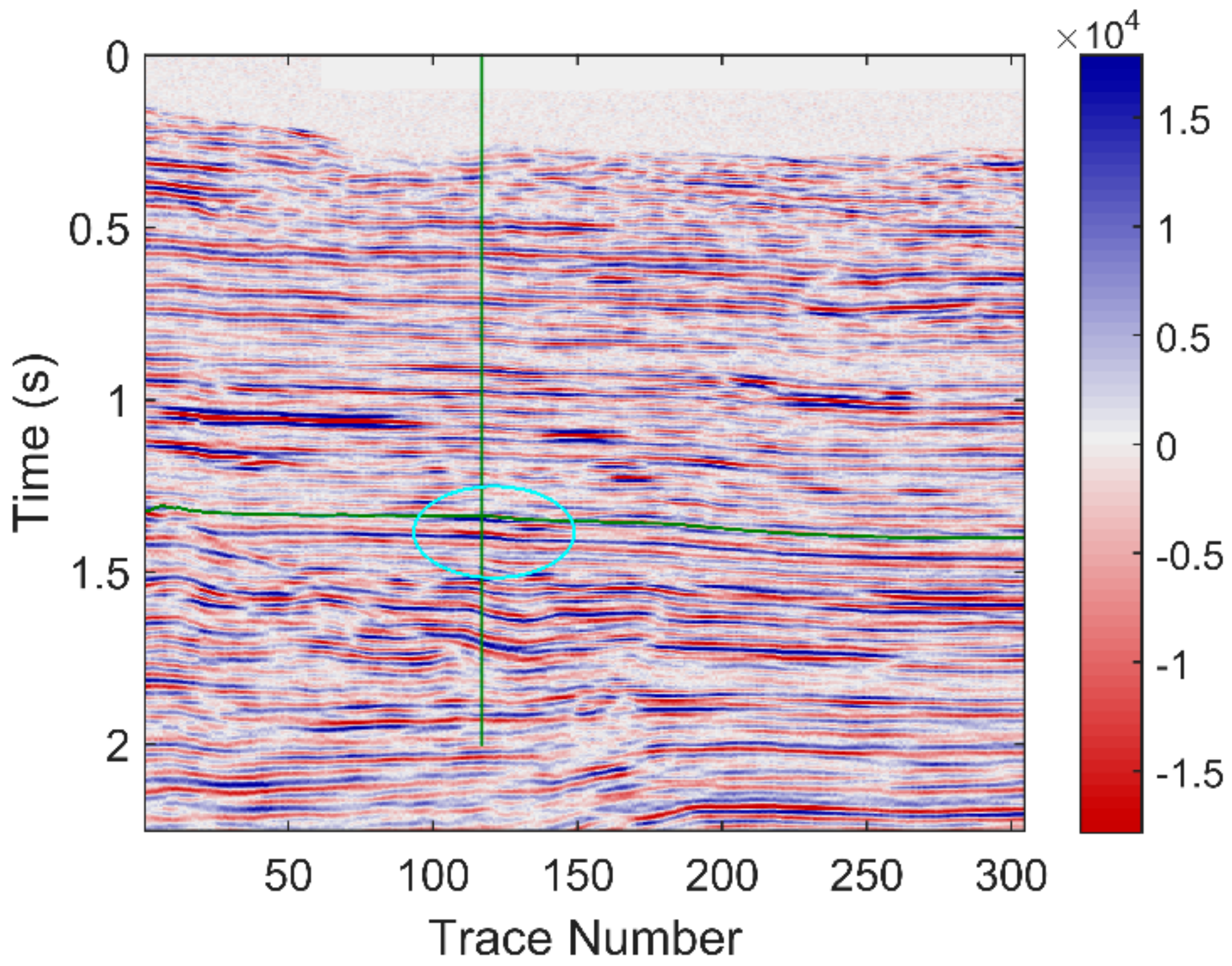
When seismic waves propagate through hydrocarbon reservoirs, waves induced by fluid flow can lead to abnormal attenuation of energy and frequency (e.g., [31,32]). The phenomenon of abnormal attenuation mainly shows the loss of high-frequency energy and the conservation of strong low-frequency energy (e.g., [33,34,35,36,37]). Spectral decomposition technology can be utilized to identify hydrocarbon reservoirs by analyzing the different frequency response characteristics among different scale geological bodies (e.g., [38]). Here, we apply the SSGST method to seismic field data from the ZhongJiang Gas Field located in the western Sichuan Basin, China, in order to identify hydrocarbon reservoirs by analyzing the abnormal instantaneous frequency and energy.
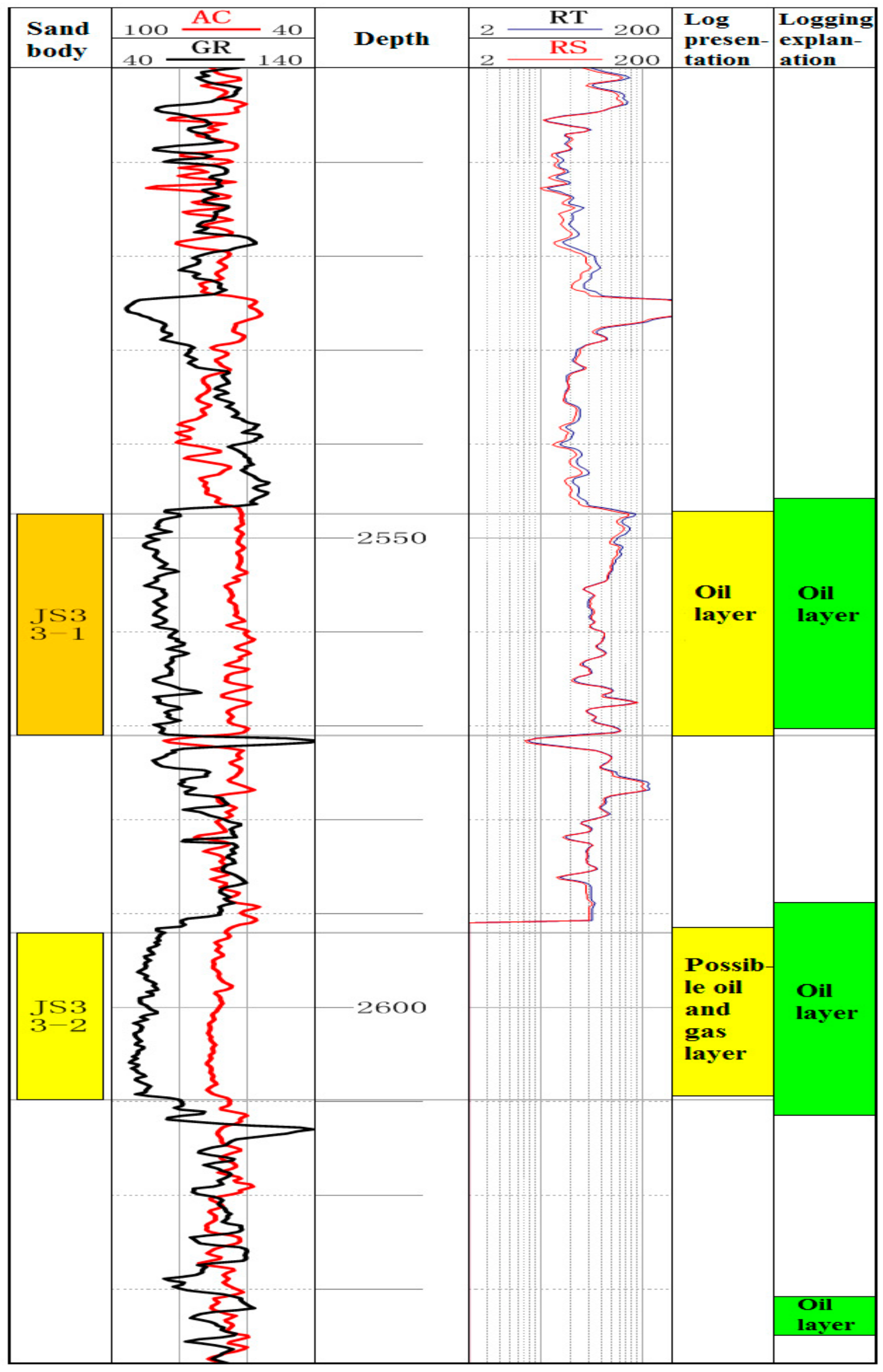
The seismic section consists of 304 traces with 1126 sampling points and a sampling interval of 2 ms, which is shown in Figure 7. The green curve in the horizontal direction at around 1.35 ms is a seismic horizon and the green vertical line represents a gas well. The area within the blue ellipse is a gas-bearing reservoir, which is our study area. Figure 8 is a histogram based on comprehensive analysis of log data. There are two sets of hydrocarbon reservoirs in the study area: the first set of reservoirs (JS33-1) is located in near a depth of 2560 m and thickness of about 22 m, and the second set of reservoirs (JS33-2) is located in near a depth of 2600 m and thickness of about 18 m.
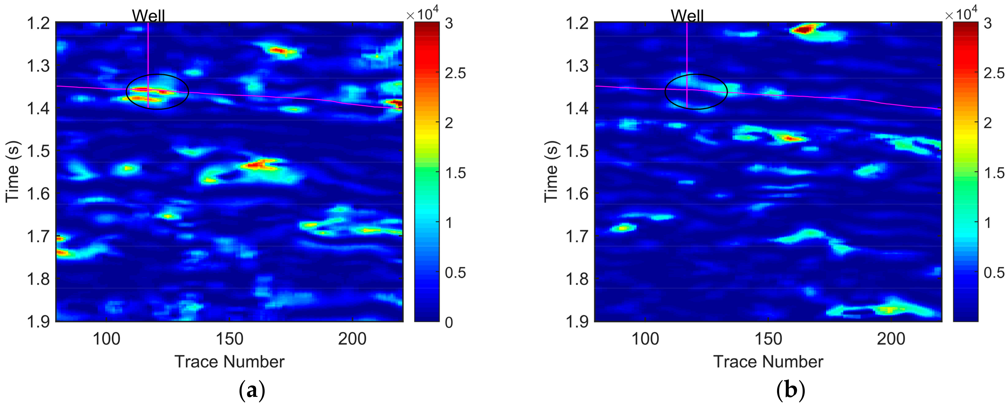
We used the CWT, GST, SSCWT, and SSGST methods respectively to processes the seismic data and extract the constant frequency sections at 40 Hz and 50 Hz, as shown in Figure 9, Figure 10, Figure 11 and Figure 12. The results are enlarged, and only the areas with time ranging from 1.2 s to 1.9 s are displayed in these constant frequency sections. In the constant frequency sections at 40 Hz (Figure 9a, Figure 10a, Figure 11a and Figure 12a), we can see a strong energy in the study area. However, obvious energy attenuation can be seen in each of the 50 Hz sections (Figure 9b, Figure 10b, Figure 11b and Figure 12b). This phenomenon is consistent with objective reality. Therefore, the four methods are all effective for hydrocarbon detection.
Although the analysis results of the CWT and GST can observe the abnormal attenuation in the hydrocarbon reservoir, they offer rough reservoir information due to the poor time-frequency resolution of CWT and GST (Figure 9 and Figure 10). Compared with the CWT and GST methods, the SSCWT method can improve the time-frequency resolution and obtain the accurate reservoir information but cannot identify the boundaries of the two sets of hydrocarbon reservoirs, as shown in Figure 11.
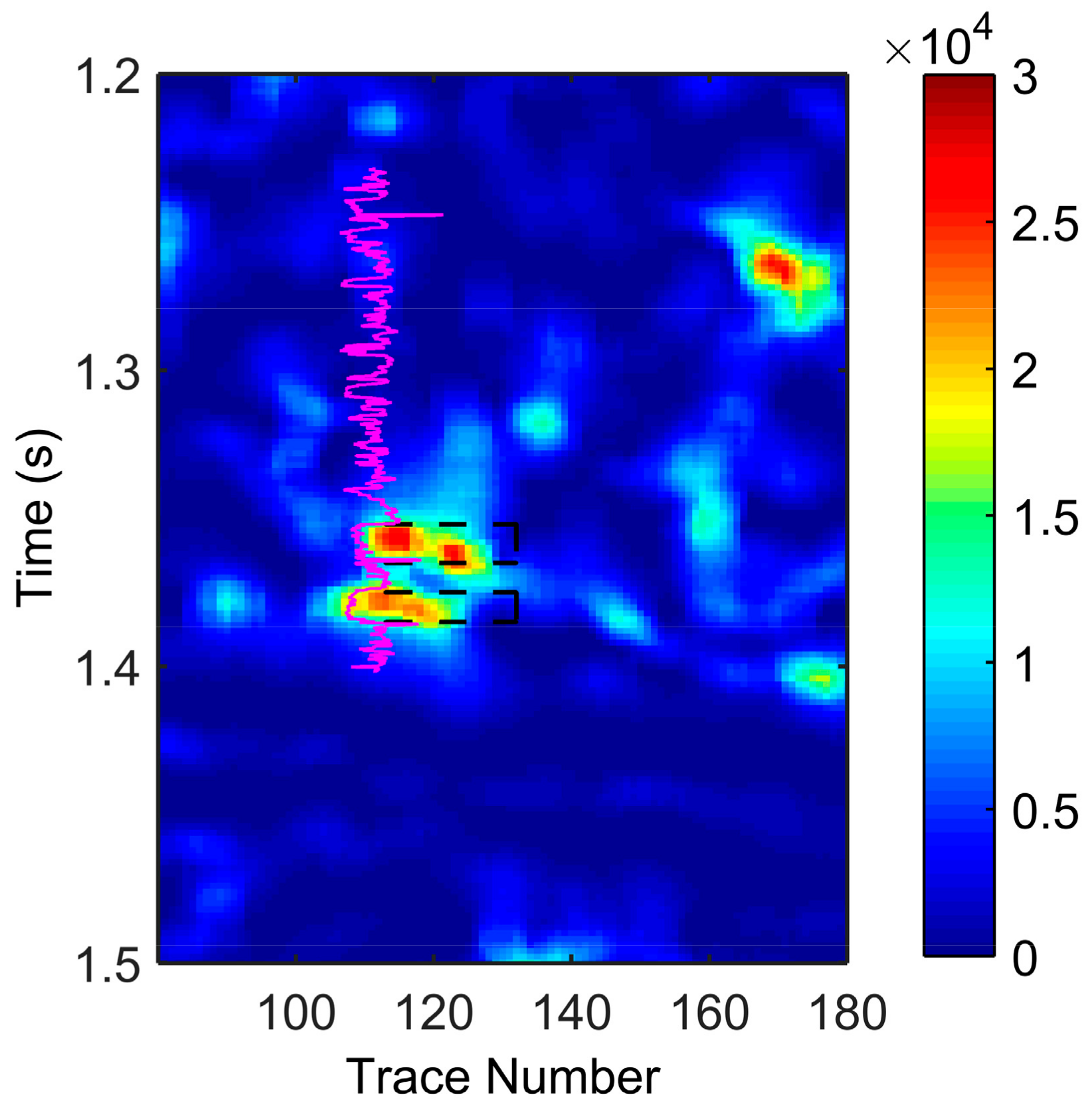
The constant frequency sections at 40 Hz and 50 Hz obtained by SSGST are shown in Figure 12. By comparing these two constant frequency sections, we can conclude that the hydrocarbon reservoir is in the elliptical area. To highlight more details about the elliptical area in Figure 12, we have locally enlarged the 40 Hz constant frequency section and combined it with the red acoustic velocity logging curve to analysis. The strong energy group in the two black-dashed, rectangular areas in Figure 13 represent the two hydrocarbon reservoirs, namely JS33-1 and JS33-2, respectively. According to the comparison with CWT, GST, and SSCWT, we can find that SSGST can provide higher time-frequency resolution and can more accurately extract the abnormal response characteristics of seismic signals. Therefore, the SSGST method can locate hydrocarbon reservoirs effectively and depicts the reservoir boundary accurately with higher precision.
5. Conclusions
A more energy-concentrated time-frequency result denotes better time-frequency location and better characterization of the time-varying feature. In this paper, the new synchrosqueezing algorithm based on the generalized S-transform (GST), namely the SSGST method, squeezes and reconstructs the complex coefficient spectra produced by the GST along the frequency direction so that the energy distributions on the time-frequency spectra are concentrated around the real instantaneous frequency of the target signal, thus showing satisfying time-frequency resolution. SSGST is a promising technique for the extraction of time-varying features of seismic signals. Results of the three synthetic examples demonstrate that the SSGST method can correctly obtain time-frequency representations of the signals and depict instantaneous frequency information better compared with CWT, GST, and SSCWT. Moreover, SSGST can reconstruct the original signal with small errors. The feasibility and validity of the SSGST method in seismic time-frequency analysis for hydrocarbon detection is confirmed via an applied example. Therefore, the SSGST method can be used as a new high-precision time-frequency analysis method in seismic signal processing and analysis.
Acknowledgments
The work presented in this paper has been supported by the National Natural Science Foundation of China (No. 41304111), key project of the Science Technology Department of Sichuan Province (No. 2016JY0200), the Natural Science project of Education Department of Sichuan Province (No. 14ZA0061, 16ZB0101 and 17ZA0030), the Sichuan Provincial Youth Science and Technology Innovative Research Group Fund (No. 2016TD0023), and the Cultivating Programme of Excellent Innovation Team of Chengdu University of Technology (No. KYTD201410).
Author Contributions
Hui Chen conceived the idea of this research. Hui Chen and Jiaxing Kang built a detail analysis framework. Jiaxing Kang, Lingqi Lu, and Dan Xu conceived, designed, and performed the experiments under the supervision of Hui Chen. Dan Xu and Xuping Chen analyzed the results and provided a detail interpretation. The paper was written by all the authors. All the authors treat the suggestions of reviewers seriously.
Conflicts of Interest
The authors declare no conflicts of interest.
References
- Mallat, S. A Wavelet Tour of Signal Processing, The Sparse Way, 3rd ed.; Academic Press: Cambridge, MA, USA, 2008. [Google Scholar]
- Stockwell, R.G.; Mansinha, L. Localization of the complex spectrum: The S transform. IEEE Trans. Signal Process. 1996, 44, 998–1001. [Google Scholar] [CrossRef]
- Zhang, X.H.; Zhao, J.M. Application of the DC Offset Cancellation Method and S Transform to Gearbox Fault Diagnosis. Appl. Sci. 2017, 7, 207. [Google Scholar] [CrossRef]
- Mcfadden, P.D.; Cook, J.G. Decomposition of gear vibration signals by the generalized S transform. Mech. Syst. Signal Process. 1999, 13, 691–707. [Google Scholar] [CrossRef]
- Pinnegar, C.R.; Mansinha, L. The S-transform with windows of arbitrary and varying shape. Geophys. 2003, 68, 381–385. [Google Scholar] [CrossRef]
- Gao, J.H.; Chen, W.C. Generalized S Transform and Seismic Response Analysis of Thin Interbeds. Chin. J. Geophys. 2003, 46, 526–532. [Google Scholar] [CrossRef]
- Sejdic, E.; Djurovic, I. A window width optimized S-transform. EURASIP J. Adv. Signal Process. 2008, 2008, 672941. [Google Scholar] [CrossRef]
- Chen, X.H.; He, Z.H. Low frequency shadow detection of gas reservoirs in time-frequency domain. Chin. J. Geophys. 2009, 52, 215–221. [Google Scholar]
- Li, D.; Castagna, J. Investigation of generalized S-transform analysis windows for time-frequency analysis of seismic reflection data. Geophys. 2016, 81. [Google Scholar] [CrossRef]
- Huang, N.E.; Shen, Z. The empirical mode decomposition and the Hilbert spectrum for nonlinear and non-stationary time series analysis. Proc. R. Soc. A 1998, 454, 903–995. [Google Scholar] [CrossRef]
- Battista, B.M.; Knapp, C. Application of the empirical mode decomposition and Hilbert-Huang transform to seismic reflection data. Geophysics 2007, 72, H29–H37. [Google Scholar] [CrossRef]
- Huang, J.W.; Milkereit, B. Empirical mode decomposition based instantaneous spectral analysis and its applications to heterogeneous petrophysical model construction. In Proceedings of the CSPG CSEG CWLS Convention, Calgary, AB, Canada, 4–8 May 2009; pp. 205–210. [Google Scholar]
- Han, J.J.; van der Baan, M. Empirical mode decomposition for seismic time-frequency analysis. Geophysics 2013, 78, O9–O19. [Google Scholar] [CrossRef]
- Xue, Y.J.; Cao, J.X. Application of the empirical mode decomposition and wavelet transform to seismic reflection frequency attenuation analysis. J. Petrol. Sci. Eng. 2014, 122, 360–370. [Google Scholar] [CrossRef]
- Tary, J.B.; Baan, M.V.D. Attenuation estimation using high resolution time–frequency transforms. Digit. Signal Process. 2017, 60, 46–55. [Google Scholar] [CrossRef]
- Auger, F.; Flandrin, P. Time-frequency reassignment and synchrosqueezing: An overview. IEEE Signal Process. Mag. 2013, 30, 32–41. [Google Scholar] [CrossRef] [Green Version]
- Thakur, G.; Wu, H.T. Synchrosqueezing-based Recovery of Instantaneous Frequency from Nonuniform Samples. Siam J. Math. Anal. 2011, 43, 2078–2095. [Google Scholar] [CrossRef]
- Oberlin, T.; Meignen, S. The Fourier-based synchrosqueezing transform. In Proceedings of the 2014 IEEE International Conference on Acoustics, Speech and Signal Processing (ICASSP), Florence, Italy, 4–9 May 2014; pp. 315–319. [Google Scholar]
- Iatsenko, D.; McClintock, P.V. Linear and synchrosqueezed time–frequency representations revisited: Overview, standards of use, resolution, reconstruction, concentration, and algorithms. Digit. Signal Process. 2015, 42, 1–26. [Google Scholar] [CrossRef] [Green Version]
- Yang, H.Z. Synchrosqueezed wave packet transforms and diffeomorphism based spectral analysis for 1D general mode decompositions. Appl. Comput. Harmon. Anal. 2015, 39, 33–66. [Google Scholar] [CrossRef]
- Yang, H.Z.; Ying, L.X. Synchrosqueezed Curvelet Transform for two-dimensional Mode Decomposition. Siam J. Math. Anal. 2014, 46, 2052–2083. [Google Scholar] [CrossRef]
- Huang, Z.L.; Zhang, J.Z. Synchrosqueezing S-Transform and Its Application in Seismic Spectral Decomposition. IEEE Trans. Geosci. Remote Sens. 2016, 54, 817–825. [Google Scholar] [CrossRef]
- Thakur, G.; Brevdo, E. The synchrosqueezing algorithm for time-varying spectral analysis: Robustness properties and new paleoclimate applications. Signal Process. 2013, 93, 1079–1094. [Google Scholar] [CrossRef]
- Daubechies, I.; Lu, J.F. Synchrosqueezed wavelet transforms: an empirical mode decomposition-like tool. Appl. Comput. Harmon. Anal. 2011, 30, 243–261. [Google Scholar] [CrossRef]
- Herrera, R.H.; Han, J.J. Applications of the synchrosqueezing transform in seismic time-frequency analysis. Geophysics 2014, 79, V55–V64. [Google Scholar] [CrossRef]
- Herrera, R.H.; Tary, J.B. Body Wave Separation in the Time-Frequency Domain. IEEE Geosci. Remote Sens. Lett. 2015, 12, 364–368. [Google Scholar] [CrossRef]
- Mousavi, S.M.; Langston, C.A. Automatic microseismic denoising and onset detection using the synchrosqueezed continuous wavelet transform. Geophysics 2016, 81, V341–V355. [Google Scholar] [CrossRef]
- Mousavi, S.M.; Langston, C.A. Automatic noise-removal/signal-removal based on general-cross-validation thresholding in synchrosqueezed domains, and its application on earthquake data. Geophysics 2017, 82, 1–58. [Google Scholar] [CrossRef]
- Tary, J.B.; Mirko, V.D.B. Applications of high-resolution time-frequency transforms to attenuation estimation. Geophysics 2017, 82, V7–V20. [Google Scholar] [CrossRef]
- Yu, G.; Yu, M. Synchroextracting Transform. IEEE Trans. Ind. Electron. 2017. [Google Scholar] [CrossRef]
- Müller, T.M.; Gurevich, B. Seismic wave attenuation and dispersion resulting from wave-induced flow in porous rocks—A review. Geophysics 2010, 75, 75A:147–75A:164. [Google Scholar] [CrossRef]
- Yin, X.Y.; Zong, Z.Y. Research on seismic fluid identification driven by rock physics. Sci. Chin. 2015, 58, 159–171. [Google Scholar] [CrossRef]
- Taner, M.T.; Koehler, F. Complex seismic trace analysis. Geophysics 1979, 44, 1041–1063. [Google Scholar] [CrossRef]
- Castagna, J.P.; Sun, S. Instantaneous spectral analysis: Detection of low-frequency shadows associated with hydrocarbons. Lead. Edge 2003, 22, 120–127. [Google Scholar] [CrossRef]
- Xiong, X.J.; He, X.L. High-precision frequency attenuation analysis and its application. Appl. Geophys. 2011, 8, 337–343. [Google Scholar] [CrossRef]
- Xue, Y.J.; Cao, J.X. EMD and Teager–Kaiser energy applied to hydrocarbon detection in a carbonate reservoir. Geophys. J. Int. 2014, 197, 277–291. [Google Scholar] [CrossRef]
- Liu, W.; Cao, S.Y. Seismic Time–Frequency Analysis via Empirical Wavelet Transform. IEEE Geosci. Remote Sens. Lett. 2016, 13, 28–32. [Google Scholar] [CrossRef]
- Partyka, G.; Gridley, J. Interpretational applications of spectral decomposition in reservoir characterization. Lead. Edge 1999, 18, 353–360. [Google Scholar] [CrossRef]
Figure 1.
The double linear chirped signal.

Figure 2.
Time-frequency spectra of the double linear chirped signal based on (a) Continuous Wavelet Transform (CWT), (b) Generalized S-transform (GST), (c) Synchrosqueezing continuous wavelet transform (SSCWT), and (d) Synchrosqueezing generalized S-transform (SSGST).
Figure 2.
Time-frequency spectra of the double linear chirped signal based on (a) Continuous Wavelet Transform (CWT), (b) Generalized S-transform (GST), (c) Synchrosqueezing continuous wavelet transform (SSCWT), and (d) Synchrosqueezing generalized S-transform (SSGST).
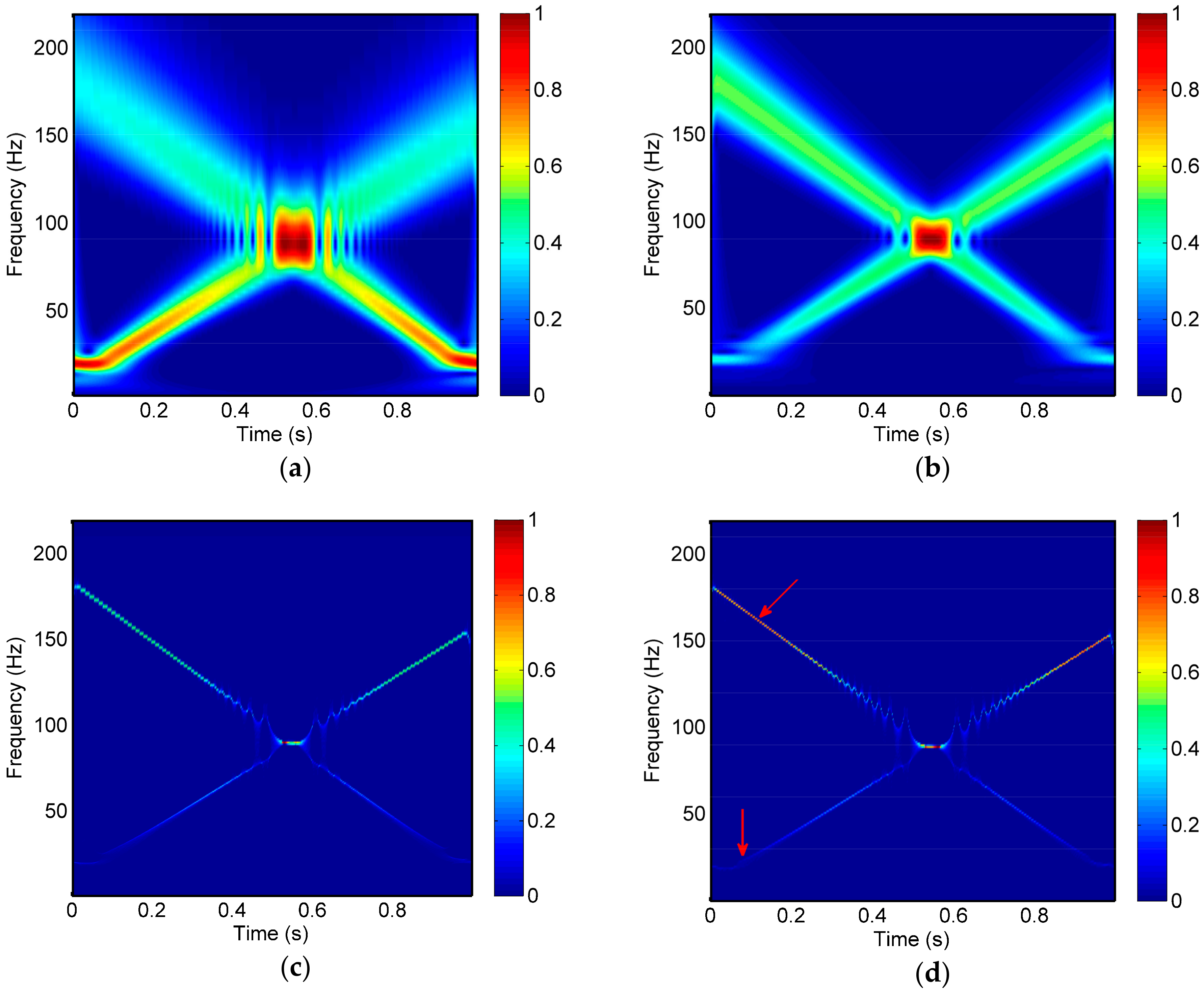
Figure 3.
The double hyperbolic chirped signal.

Figure 4.
Time-frequency spectra of the double hyperbolic chirped signal based on (a) CWT, (b) GST, (c) SSCWT, and (d) SSGST.
Figure 4.
Time-frequency spectra of the double hyperbolic chirped signal based on (a) CWT, (b) GST, (c) SSCWT, and (d) SSGST.
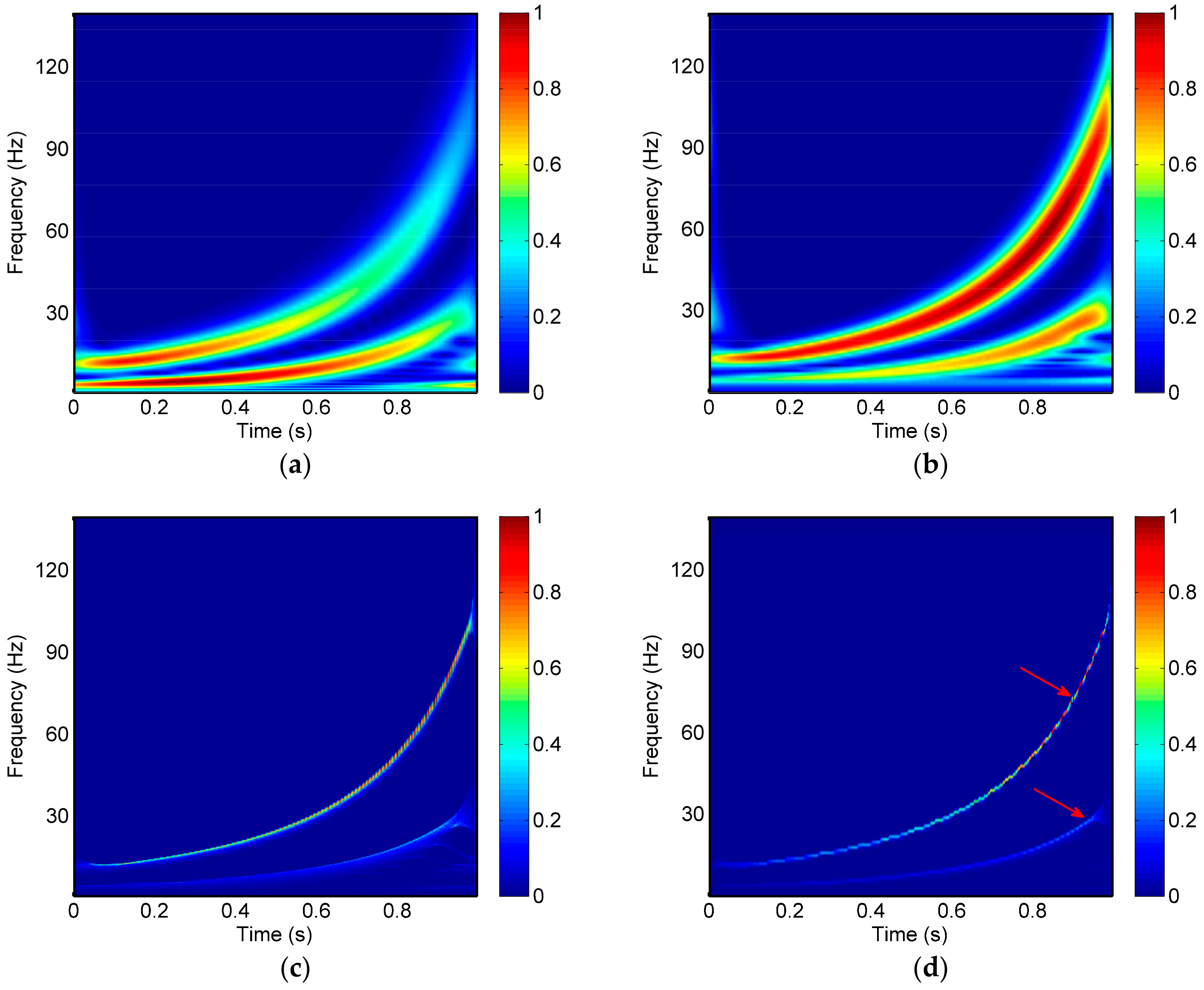
Figure 5.
The components of the synthetic signal.

Figure 6.
Time-frequency spectra of the synthesized signal based on (a) CWT; (b) GST; (c) SSCWT; (d) SSGST.
Figure 6.
Time-frequency spectra of the synthesized signal based on (a) CWT; (b) GST; (c) SSCWT; (d) SSGST.
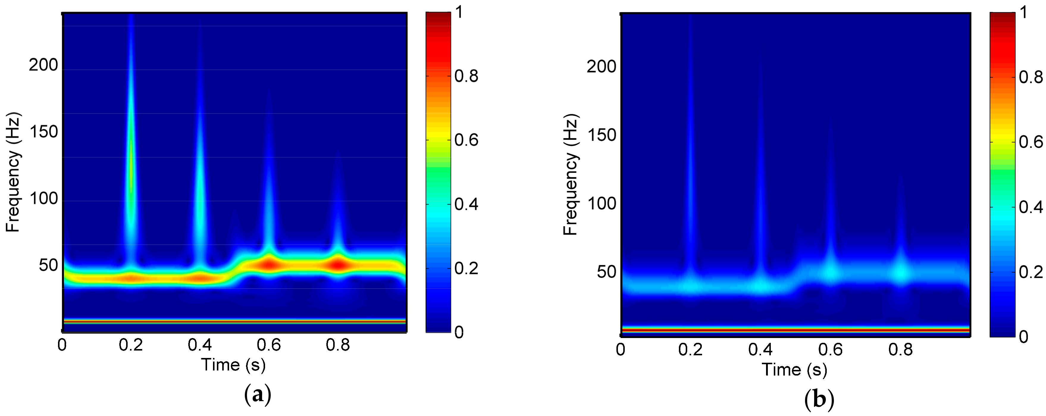

Figure 7.
The seismic section from the ZhongJiang Gas Field.

Figure 8.
Histogram from the comprehensive analysis of well data (The red curve on the left is acoustic log (AC), and the unit of AC is us/ft. The black curve is natural gamma ray log (GR), and the unit of GR is API. The blue curve is true formation resistivity log (RT), and the unit of RT is OMM. The red curve on the right is shallow investigate double lateral resistivity log (RS), and the unit of RS is OMM.).

Figure 9.
Constant frequency sections based on CWT (a) at 40 Hz and (b) at 50 Hz.
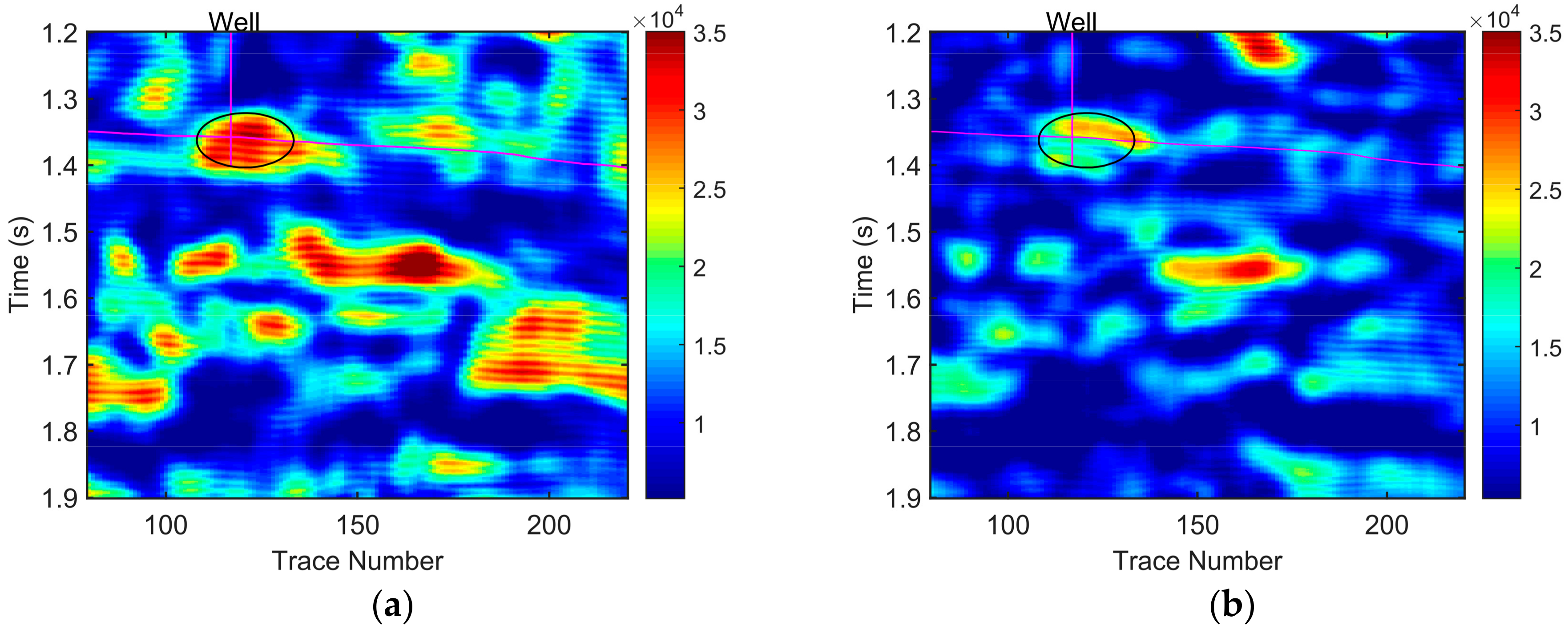
Figure 10.
Constant frequency sections based on GST (a) at 40 Hz and (b) at 50 Hz.
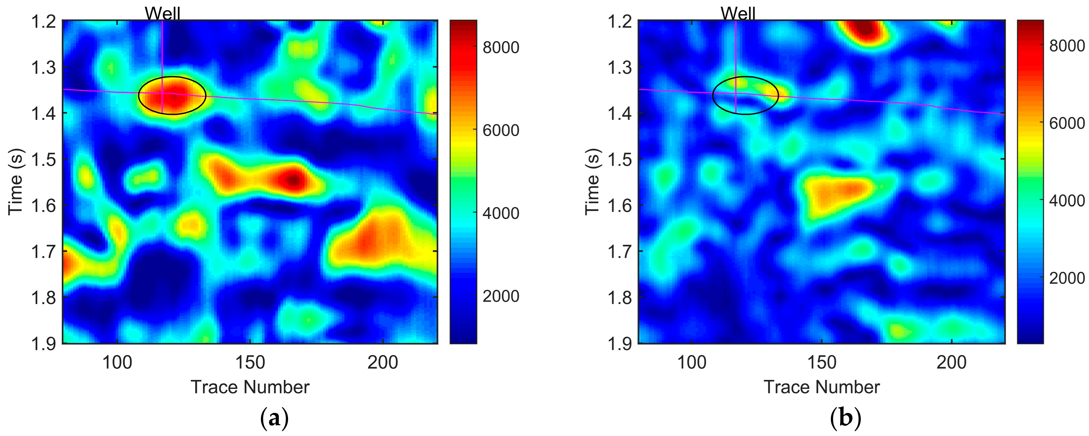
Figure 11.
Constant frequency sections based on SSCWT (a) at 40 Hz and (b) at 50 Hz.
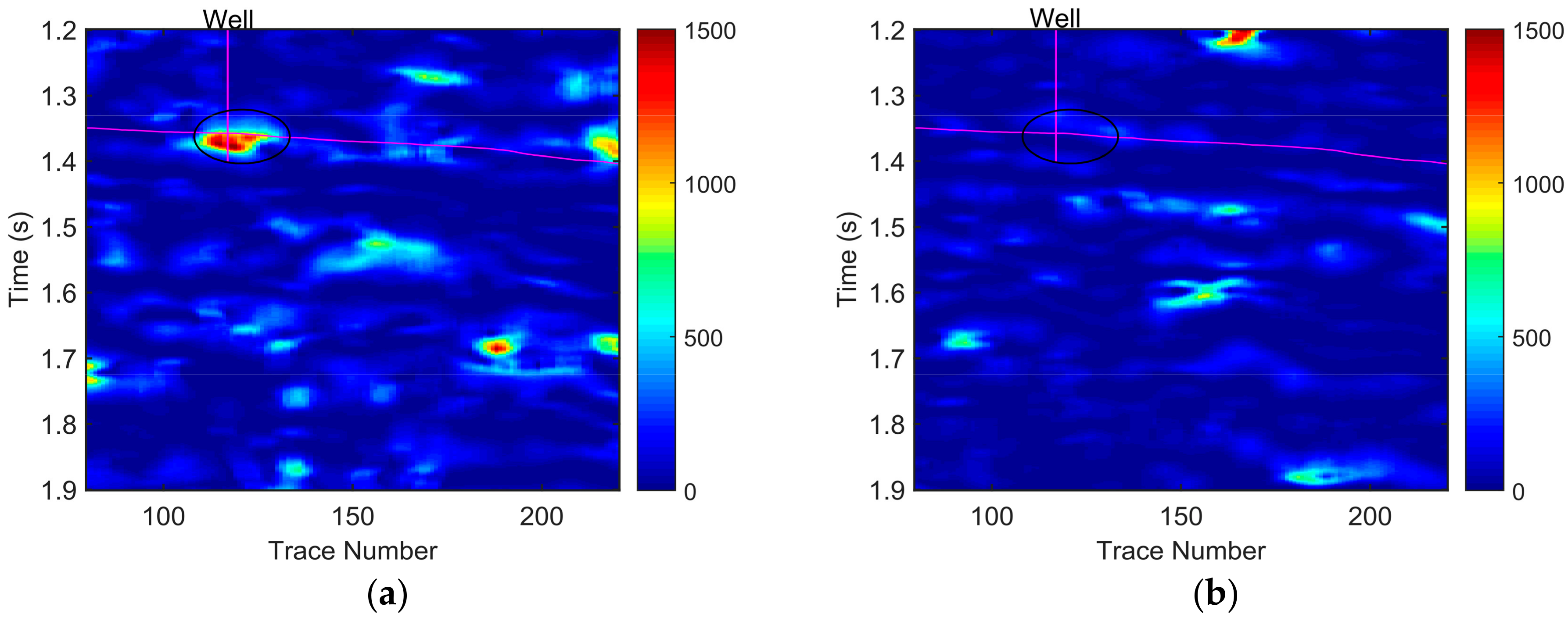
Figure 12.
Constant frequency sections based on SSGST (a) at 40 Hz and (b) at 50 Hz.

Figure 13.
The details of Figure 12a near hydrocarbon reservoir.
Figure 13.
The details of Figure 12a near hydrocarbon reservoir.

Table 1.
The Rényi Entropies of three synthetic examples based on the Continuous Wavelet Transform (CWT), Generalized S-transform (GST), Synchrosqueezing continuous wavelet transform (SSCWT), and Synchrosqueezing Generalized S-transform (SSGST) methods. Signal1 is the double hyperbolic chirped signal. Signal2 is the double hyperbolic chirped signal. Signal3 is the synthesized signal.
| Rényi Entropy | CWT | GST | SSCWT | SSGST |
|---|---|---|---|---|
| Signal1 | 5.1846 | 6.0156 | 2.3329 | 1.1779 |
| Signal2 | 6.6262 | 4.9479 | 1.6304 | 0.8297 |
| Signal3 | 7.0540 | 5.0889 | 1.2518 | 1.4250 |
Table 2.
The mean square error (MSE) values of synthetic examples based on the Synchrosqueezing Generalized S-transform (SSGST) and the other algorithms.
Table 2.
The mean square error (MSE) values of synthetic examples based on the Synchrosqueezing Generalized S-transform (SSGST) and the other algorithms.
| MSE | CWT | GST | SSCWT | SSGST |
|---|---|---|---|---|
| Signal1 | 0.0121 | 3.6979 × 10⁻²⁷ | 2.3060 × 10⁻⁵ | 1.8626 × 10⁻⁵ |
| Signal2 | 0.0181 | 3.2963 × 10⁻²⁷ | 0.0214 | 0.0083 |
| Signal3 | 0.0221 | 5.0622 × 10⁻²⁶ | 7.5347 × 10⁻⁸ | 1.0925 × 10⁻⁴ |
© 2017 by the authors. Licensee MDPI, Basel, Switzerland. This article is an open access article distributed under the terms and conditions of the Creative Commons Attribution (CC BY) license (http://creativecommons.org/licenses/by/4.0/).
Share and Cite
MDPI and ACS Style
Chen, H.; Lu, L.; Xu, D.; Kang, J.; Chen, X. The Synchrosqueezing Algorithm Based on Generalized S-transform for High-Precision Time-Frequency Analysis. Appl. Sci. 2017, 7, 769. https://doi.org/10.3390/app7080769
AMA Style
Chen H, Lu L, Xu D, Kang J, Chen X. The Synchrosqueezing Algorithm Based on Generalized S-transform for High-Precision Time-Frequency Analysis. Applied Sciences. 2017; 7(8):769. https://doi.org/10.3390/app7080769
Chicago/Turabian StyleChen, Hui, Lingqi Lu, Dan Xu, Jiaxing Kang, and Xuping Chen. 2017. "The Synchrosqueezing Algorithm Based on Generalized S-transform for High-Precision Time-Frequency Analysis" Applied Sciences 7, no. 8: 769. https://doi.org/10.3390/app7080769
Note that from the first issue of 2016, this journal uses article numbers instead of page numbers. See further details here.