Dynamic Performance Analysis for an Absorption Chiller under Different Working Conditions

Beijing Key Laboratory of Indoor Air Quality Evaluation and Control, Department of Building Science, Tsinghua University, Beijing 100084, China
*
Author to whom correspondence should be addressed.
Appl. Sci. 2017, 7(8), 797; https://doi.org/10.3390/app7080797
Submission received: 4 July 2017
/
Revised: 31 July 2017
/
Accepted: 31 July 2017
/
Published: 5 August 2017
(This article belongs to the Special Issue Sciences in Heat Pump and Refrigeration)
Abstract
:Featured Application
The dynamic performance of the absorption chiller (AC) under different working conditions in this work is significant for the operation of the whole system, of which the stabilization can be affected by the AC transient process.
Abstract
Due to the merits of energy saving and environmental protection, the absorption chiller (AC) has attracted a lot of attention, and previous studies only concentrated on the dynamic response of the AC under a single working condition. However, the working conditions are usually variable, and the dynamic performance under different working conditions is beneficial for the adjustment of AC and the control of the whole system, of which the stabilization can be affected by the AC transient process. Therefore, the steady and dynamic models of a single-effect H2O-LiBr absorption chiller are built up, the thermal inertia and fluid storage are also taken into consideration. And the dynamic performance analyses of the AC are completed under different external parameters. Furthermore, a whole system using AC in a process plant is analyzed. As a conclusion, the time required to reach a new steady-state (relaxation time) increases when the step change of the generator inlet temperature becomes large, the cooling water inlet temperature rises, or the evaporator inlet temperature decreases. In addition, the control strategy considering the AC dynamic performance is favorable to the operation of the whole system.
1. Introduction
With the speed-up of urbanization, the energy consumption of air conditioning and refrigeration keeps increasing continuously [1]. The vapor compression chiller is widely applied due to its attractive advantages, such as high efficiency, low costs, quick response time, etc. [2,3]. But it usually consumes a significant quantity of high-grade electricity, and large-scale application can cause overload of electricity generation and transmission [4]. As a potential solution to the energy and environmental problems, the absorption chiller (AC), which is mainly driven by fossil fuel, renewable energy or low-grade waste heat, is being more and more popular [5,6]. Moreover, AC has a competitive primary energy efficiency compared to electricity-driven chiller, and can adopt environmentally friendly working fluids, such as H2O-LiBr and NH3-H2O [7].
A number of researchers have studied the steady-state performance of AC by both theoretical simulations [8,9,10] and experiments [11,12,13,14]. However, the real-time operation of a commercial AC is governed by continuous transient processes, and the relaxation time required to achieve a new steady-state is rather long compared to the vapor compression chiller with a similar cooling capacity [15,16]. What’s more, the dynamic process of AC is essential for the adjustment of AC and the control of the whole system, of which the stabilization can be affected by the transient process. Under this circumstance, the dynamic performance of AC has been studied, including various working fluids like H2O-LiBr [17], NH3-H2O [18] and CO2-[bmim][PF6] [19], different absorption cycles like double-effect AC [20] and diffusion AC [21], as well as alternative method like exergy analysis [22].
Butz and Stephan [23] developed a dynamic model of an absorption heat pump, the heat source flow rate had a ±20% stepwise change, and the heat sink inlet temperature linearly increases 5 K within 300 s. The accuracy of the model was good as compared with a real machine. Jeong et al. [24] carried out the numerical simulations of a steam-driven absorption heat pump recovering waste heat, the storage terms in the model included the thermal capacities of the containers and the solution mass storage in the vessels, but lacked the thermal inertia of the heat exchangers. During the shut-off period of the system, the simulated values of the absorption heat, condensation heat and evaporation heat showed good agreement with the operational data. Kohlenbach and Ziegler [16,25] established a dynamic model of an absorption chiller, which considered the transport delays of the solution cycle, thermal storage and mass storage. The thermal capacities of all the components were divided into internal and external parts. The work also analyzed the effects of the thermal storage and transport delay on the relaxation time. But the model was a little over-simplified, since the evaporation latent heat, sorption latent heat and weak solution mass flow rate were all considered as constants. Evola et al. [26] presented a dynamic model and its experimental verification for a single-effect absorption chiller, taking into account the thermal inertia of the heat exchangers, containers and solution storage. The largest relative error between the model and experiment was ±5%. And a 10 K step change of the driving temperature was investigated. However, the cumulated heat capacities of all components, which should vary with the fluid storage, were considered as constants in this work. Ochoa et al. [15,27] completed the dynamic analysis on an absorption chiller, which considered the mass, species and energy balance. The convective coefficients were calculated with the mathematical correlations to determine the variable overall heat transfer coefficients by updating the thermal and physical properties in time. Comparing the model with the experiment, the maximum relative errors were 5% in the chilled water circuit and within 0.3% in the cold water cycle, respectively. But the heat exchange efficiency of the economizer was unchangeable in this work.
Nevertheless, previous studies [15,16,25,26,27] only concentrated on the dynamic response under a single working condition. They didn’t show how long it takes to reach a new steady-state, for example, under different cooling water temperatures. However, this is important for the adjustment of AC and the control of the whole system, because the working conditions are usually variable. Towards this end, the objective of this work is to conduct dynamic performance analyses for single-effect AC under different working conditions, including different generator inlet temperatures, cooling water inlet temperatures and evaporator inlet temperatures.
2. Principle
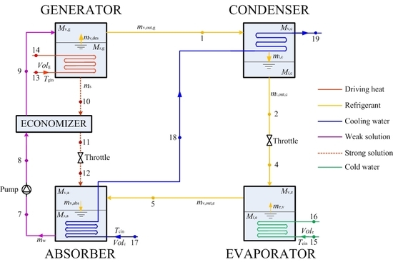
The single-effect AC is shown in Figure 1, with H2O-LiBr as the working fluid. The driving heat (point 13, 14) is supplied to the generator, desorbing the refrigerant vapor (point 1) from the solution. Then, the vapor becomes liquid (point 2) in the condenser, and the condensation heat is transferred to the cooling water (point 18, 19). Subsequently, the refrigerant is throttled by the valve and reaches the evaporator (point 4). And then, it evaporates to extract heat from outside (point 15, 16), producing a cooling effect. Finally, the refrigerant vapor arrives in the absorber (point 5) to complete an absorption process.
In the meanwhile, the strong solution leaving the generator (point 10) passes through the economizer (point 11) and the throttle valve, also reaching the absorber (point 12). In the absorber, the strong solution becomes weak solution (point 7) by absorbing refrigerant vapor, and the cooling water removes the released absorption heat (point 17, 18). Thereafter, the pressure of the weak solution is increased by a pump (point 8), and then its temperature rises in the economizer (point 9). With the weak solution returning to the generator, the next circulation repeats.
3. Modelling
The steady and dynamic models of the single-effect AC are built up on the basis of mass, species and energy conservation. The analyses are completed using the backward difference method and the Engineering Equation Solver (EES) software, which has been used by a lot of researchers for thermal modeling of absorption systems [28,29].
3.1. Assumptions
- (1)
- There is no heat exchange between the components and the ambient;
- (2)
- The pressures in the generator and the absorber are equal to those in the condenser and the evaporator, respectively.
- (3)
- The solutions leaving the generator and the absorber, and the refrigerants at the outlet of the condenser and the evaporator are saturated;
- (4)
- The transport delays in the fluid cycles are neglected;
- (5)
- The enthalpies of the fluids at the inlet and outlet of the throttle valves are equal.
3.2. Mass and Species Conservation
The mathematical equations of the generator and the condenser are similar to those of the absorber and the evaporator, respectively. So the generator and the condenser are selected to present the detailed models, and all these equations can be extended to the absorber and the evaporator, given necessary adjustment for flow directions and fluid properties.
3.2.1. Generator
(1) In a transient process, the solution mass storage in the generator depends on the entering weak solution, leaving strong solution and the desorbed vapor refrigerant, as illustrated in Figure 1. The mass conservation equation is:
where mw is the mass flow rate of the weak solution entering the generator (point 9), kg/s; ms is the mass flow rate of the strong solution leaving the generator (point 10), kg/s; mv,des is the mass flow rate of the refrigerant desorbed from the solution, kg/s; and Ms,g is the solution storage mass in the generator, kg.
(2) The species conservation for the generator is:
where xw is the weak solution mass concentration (point 9); xs is the strong solution mass concentration (point 10).
The properties of the fluids stored in the containers are assumed to be same as those of the leaving fluids [16,26].
(3) For the vapor in the generator, the mass conservation equation is:
where mv,out,g is the mass flow rate of the refrigerant leaving the generator (point 1), kg/s; and Mv,g is the refrigerant vapor storage in the generator, kg.
(4) The volume of the solution storage plus that of the vapor storage is the volume of the whole generator:
where and are the densities of the solution and the vapor stored in the generator, kg/m3; and Vg is the generator volume, m3.
(5) The volumetric flow rate of the weak solution (Volw, point 7) conveyed by the pump is set as a constant, while the strong solution flow rate is determined by the pressure and the height difference between the generator and the absorber [16,26]:
where Cd is the discharge coefficient; Sg is the valve section area between the generator and the absorber, m2; and are the pressures in the generator and the absorber, Pa; g is gravitational acceleration, m/s2; Hg is the vertical distance between the bottom of the generator and the solution inlet of the absorber, m; and ζg is the resistance coefficient indicating the pressure losses in the valve and the pipes.
where is the solution height inside the generator, which is calculated by:
where Ag is the bottom area of the generator, m2.
3.2.2. Condenser
For the condenser, the principle is similar, but these equations are simpler, since there is only one species.
(1) Vapor storage equation:
where ml,c is the mass flow rate of the refrigerant condensed from the vapor in the condenser, kg/s; and Mv,c is the refrigerant vapor storage in the condenser, kg.
(2) Liquid storage equation:
where ml,out,c is the mass flow rate of the refrigerant liquid leaving the condenser (point 2), kg/s; and Ml,c is the refrigerant liquid storage in the condenser, kg.
(3) The condenser is also filled with liquid and vapor:
where and separately are the densities of the vapor and the liquid stored in the condenser, kg/m3; and Vc is the condenser volume, m3.
(4) The mass flow rate of the refrigerant liquid leaving the condenser is:
where Sc is the valve section area between the condenser and the evaporator, m2; Hc is the vertical distance between the bottom of the condenser and the liquid inlet of the evaporator, m; and ζc is the resistance coefficient used to reflect the pressure losses in the pipes between the condenser and the evaporator.
where is the liquid height inside the condenser, and calculated by:
where Ac is the bottom area of the condenser, m2.
3.3. Energy Conservation
3.3.1. Generator
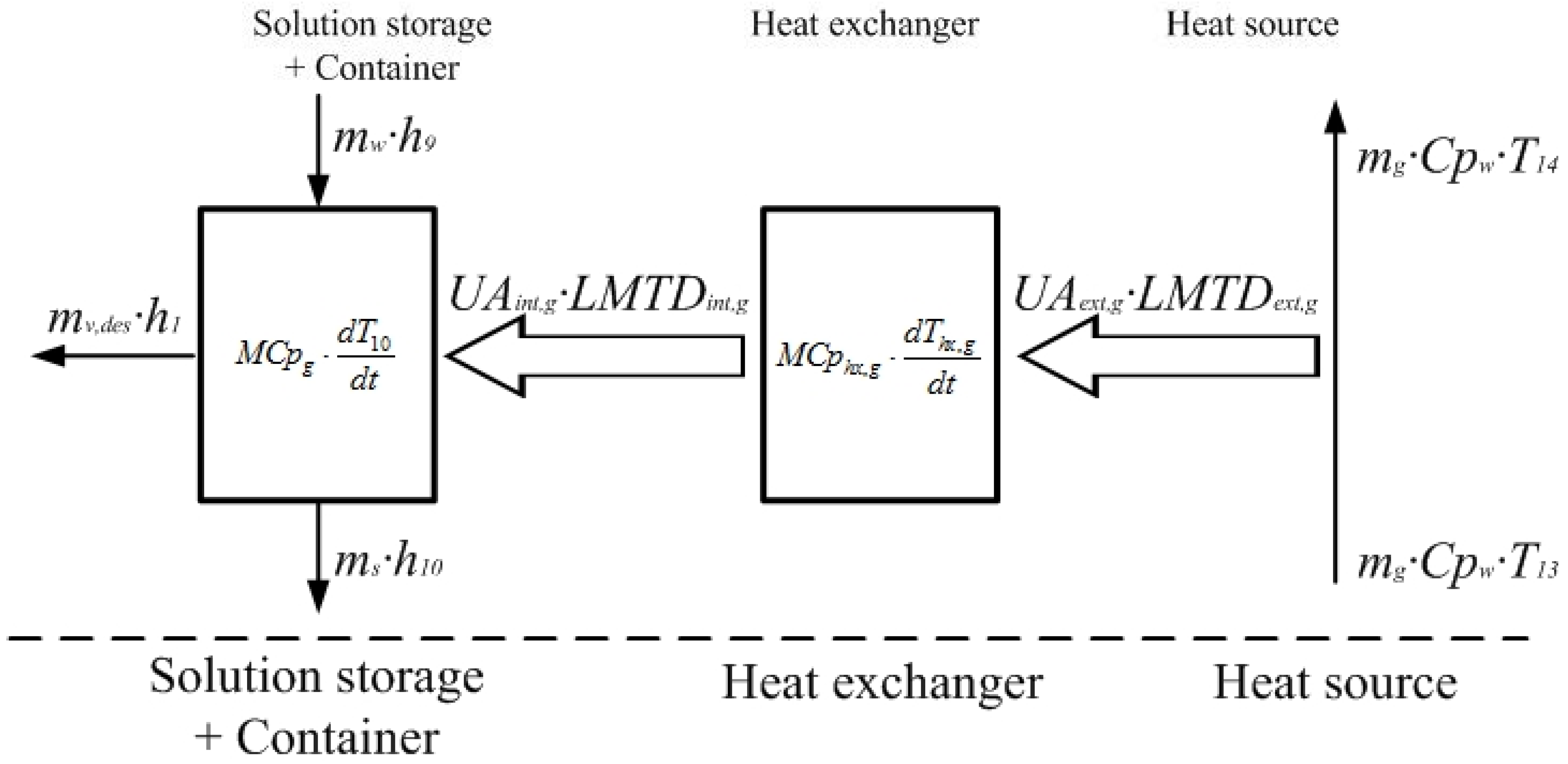
In the generator, outside heat source (point 13, 14) transfers the driving heat to the inside working fluids, as shown in Figure 2. Since there are thermal storages like the heat exchanger, the container and the solution storage, the machine needs some relaxation time to achieve a new steady-state. Thus, the thermal capacities are taken into consideration in the model.
(1) External heat exchange occurs between the driving heat source (hot water) and the heat exchanger, which is assumed to have a uniform temperature [26]. Thus, the energy balance equations are:
where Qg,ext is the external heat exchange rate in the generator, kW; Volg is the volumetric flow rate of the hot water in point 13, m3/h; . is the density of the hot water at its inlet temperature T13, kg/m3; Cpwa is the specific heat of the hot water, kJ/(kg·K); T13 is the generator inlet temperature, °C; T14 is the generator outlet temperature, °C; UAext,g is the product of the external heat transfer coefficient and external heat transfer area for the generator, kW/K; LMTDext,g is the external logarithmic mean temperature difference, °C; and Thx,g is the uniform temperature of the heat exchanger in the generator, °C.
(2) Internal heat exchange between the heat exchanger and the working fluids is:
where Qg,int is the internal heat exchange rate in the generator, kW; UAint,g is the product of the internal heat transfer coefficient and internal heat transfer area of the generator, kW/K; LMTDint,gi is the internal logarithmic mean temperature difference in the generator, °C.
(3) The difference between Qg,ext and Qg,int represents the thermal energy stored in the body of the heat exchanger.
where MCphx,g is the product of the heat exchanger mass and its specific heat in the generator, kJ/K.
(4) All the internal heat Qg,int is not used for the generation process; part of it is applied to raise the temperatures of the solution storage and container in the generator:
where MCpg is the thermal capacities of the solution storage and the container in the generator, kJ/K; MCpg,con is the product of the container mass and its specific heat in the generator, kJ/K.
The desorbed vapor temperature T1 equals to the saturation temperature associated with the weak solution entering the generator. It is between the weak solution temperature and the strong solution temperature, meaning the temperature that the refrigerant begins to be desorbed from the weak solution. The temperature of the container is set to be same with that of the solution storage [26].
3.3.2. Condenser
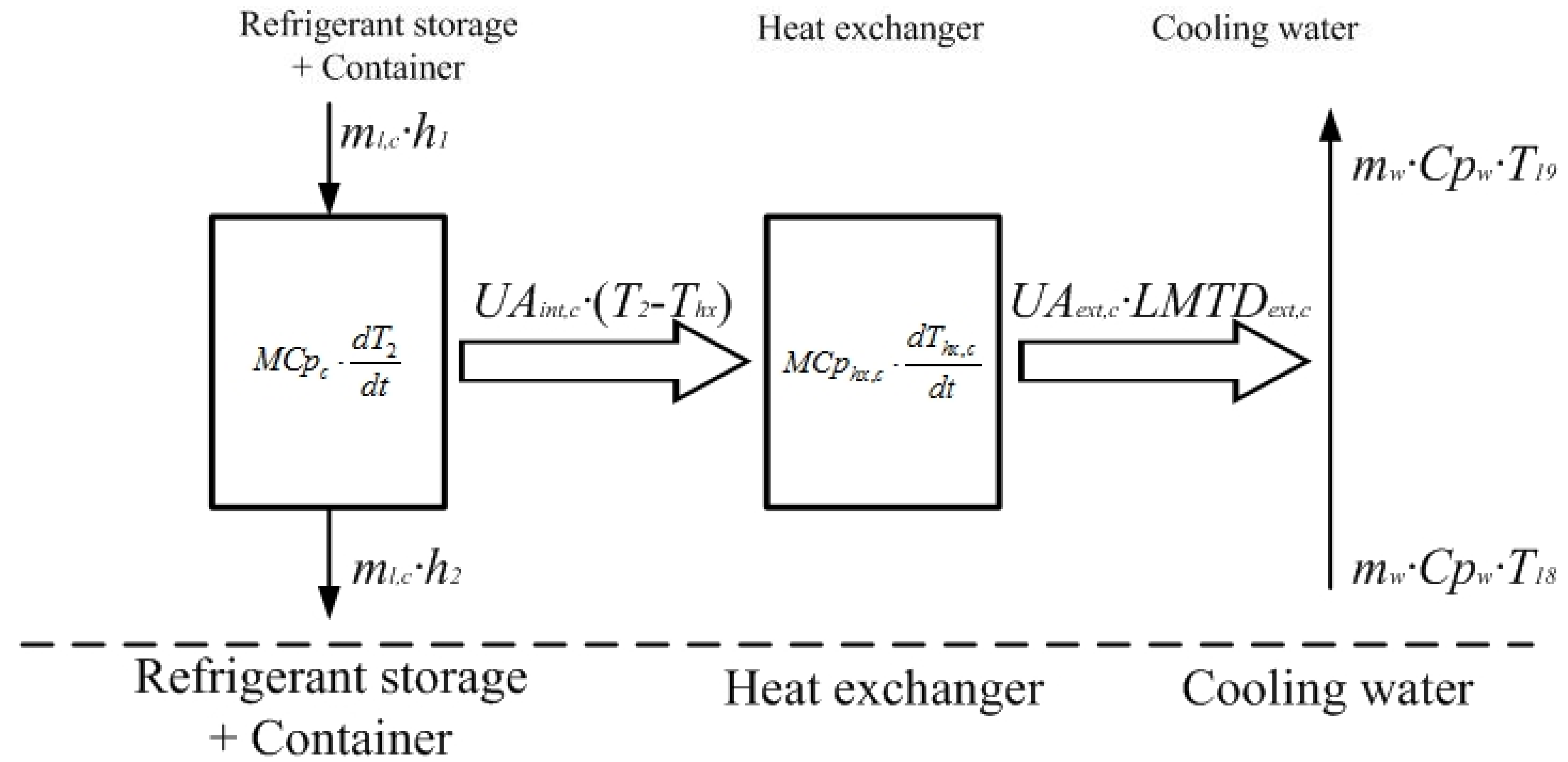
For the condenser, the heat coming from the refrigerant condensation process is taken away by the cooling water (point 18, 19), and there also exists thermal inertia, as depicted in Figure 3.
(1) The internal heat exchange between the working fluids and the heat exchanger is:
where Qc,int is the internal heat exchange rate in the condenser, kW; MCpc is the thermal capacities of the refrigerant storage and the container in the condenser, kJ/K; MCpc,con is the product of the container mass and its specific heat in the condenser, kJ/K; UAint,c is the product of the internal heat transfer coefficient and internal heat transfer area in the condenser, kW/K; Thx,c is the uniform temperature of the heat exchanger in the condenser, °C.
Because part of the condensation heat is not transferred to the outside, but stored by the refrigerant liquid storage and the container, the symbol of the last item in Equation (22) is minus.
(2) The external heat exchange equations are:
where Qc,ext is the external heat exchange rate in the condenser, kW; UAext,c is the product of the external heat transfer coefficient and external heat transfer area in the condenser, kW/K; LMTDext,g is the external logarithmic mean temperature difference in the condenser, °C; Volc is the volumetric flow rate of the cooling water in point 18, m3/h; is the density of the cooling water under its inlet temperature T18, kg/m3; T18 is the cooling water inlet temperature of the condenser, °C; T19 is the cooling water outlet temperature of the condenser, °C.
(3) The thermal energy stored on the body of the heat exchanger is:
where MCphx,c is the product of the heat exchanger mass and its specific heat in the condenser, kJ/K.
3.4. Efficiency
The dynamic coefficient of performance (COP) is:
where Qe,ext is the external heat exchange rate in the evaporator, kW.
These above formulas are for the dynamic model, but they can become the steady model when all differential items equal to zero. Some constant parameters required in these equations are shown in Table 1.
3.5. Validation of Model
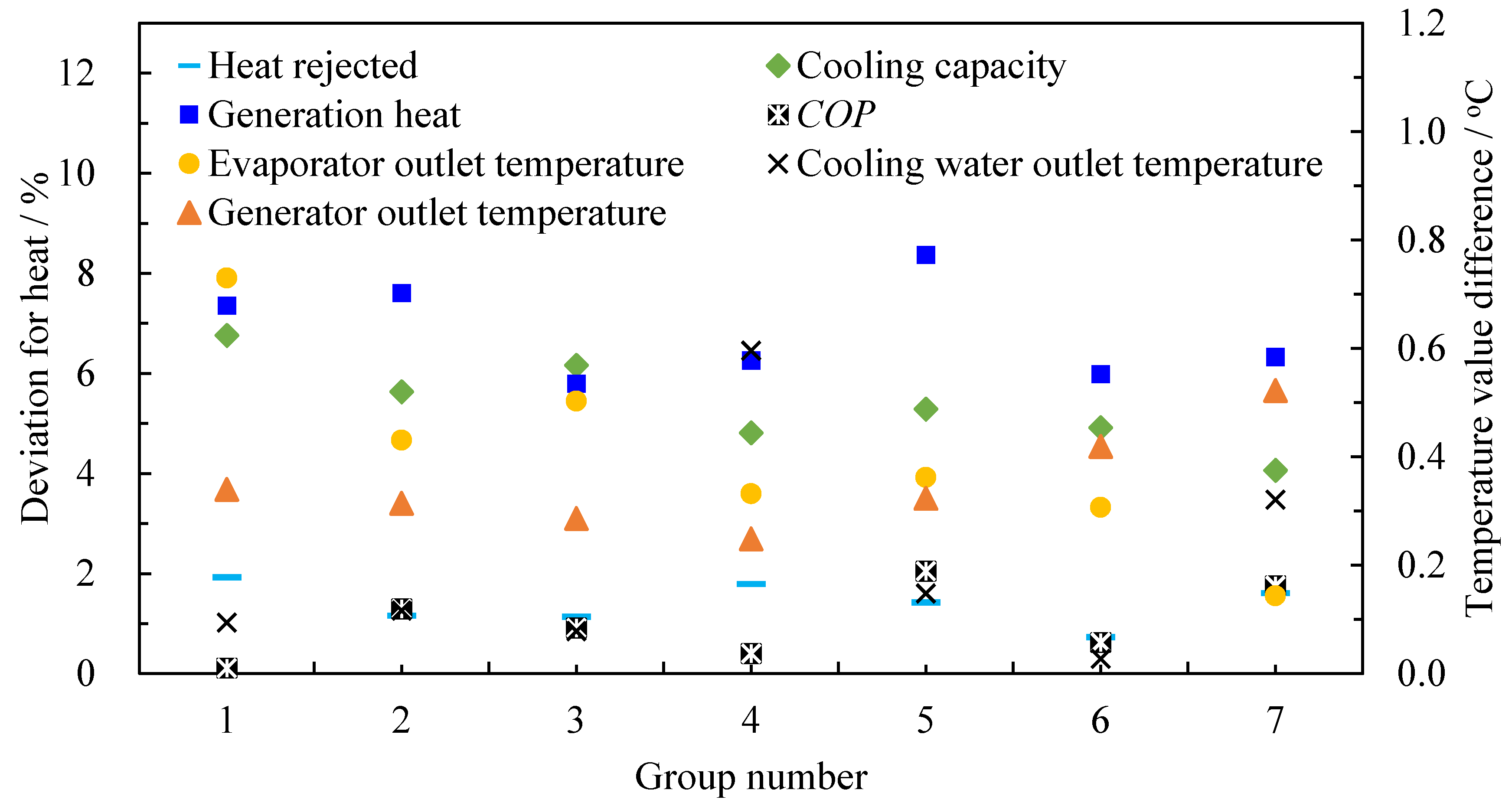
To make sure that the model has sufficient accuracy, 7 groups of experimental data, including generator inlet temperature, cooling water inlet temperature and evaporator inlet temperature of Ref. [26], are inputted into the model. Then the simulated results are compared with the data from Ref. [26]. The deviations are calculated by:
where Pa means calculated results with the present model, and Paref represents the parameters in Ref. [26].
Comparative results are shown in Figure 4, and the right vertical axis is the outlet temperature difference between the model and Ref. [26]. The deviations are small enough to prove the accuracy of the model. Although the validation is for the steady model, both the steady model and the dynamic model follow the mass and energy conservation, and the dynamic model can become the steady model when all differential items equal to zero. Therefore, this model can be used for further studies.
4. Dynamic Performance Analysis
The following content concerns the dynamic performance of the absorption chiller under different working conditions, which is essential for the adjustment of AC and the stabilization of the whole system, which includes the AC. The steady-state judgment criterion is:
where Qe,st is the cooling capacity on steady-state after the dynamic process, which is obtained from the steady model, kW; Qe,ext,i is the external heat exchange rate in the evaporator at time i, which is calculated with the dynamic model, kW.
The dynamic process ends when the δQe,i is smaller than 0.2%, and the time interval i is called as relaxation time.
4.1. Generator Inlet Temperature (Tgin)
4.1.1. Dynamic Response Process
To investigate the effects of the mass and thermal storage, a step change of 10 °C (from 90 °C to 100 °C) for Tgin appears at time 0, and then the dynamic response of the AC is observed and shown in Figure 5. In the meanwhile, the cooling water inlet temperature Tcin and the evaporator inlet temperature Tein remain at 32 °C and 12 °C, respectively.
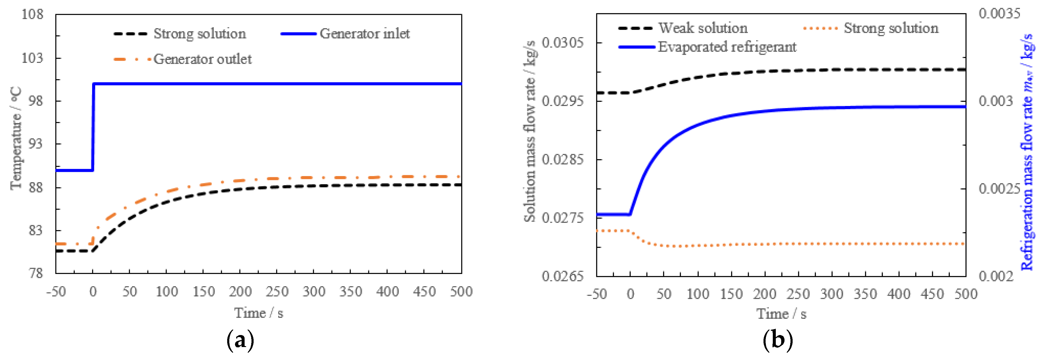
At the beginning, the AC is on steady-state, but the generator inlet temperature Tgin increases by 10 °C steeply at time 0 in Figure 5a, resulting in gradually growing for both the generator outlet temperature and the strong solution temperature. So, the solution concentration difference in Figure 5d and the evaporated refrigerant mass flow rate me,v in Figure 5b become large. The strong solution mass flow rate decreases at first because of the increased refrigerant. However, the solution density becomes high with the rising concentration, so a slight inversion trend appears in the curve after 100 s in Figure 5b. The volumetric flow rate of the weak solution is constant, but its density also grows, thus the mass flow rate increases gradually.
In Figure 5c, all the external heat exchange rates of the condenser, the evaporator and the absorber keep rising as a consequence of more refrigerant production. And the temperature steep change is followed by a steep increase of the external generation heat Qg,ext,i due to the improved temperature difference in the generator. Accordingly, the COPi initially shows a sudden decrease in Figure 5d. Nevertheless, such a fall can be recovered progressively as long as the Qg,ext,i decreases and Qe,ext,i increases. Finally, all these parameters reach a new steady-state, and their values are almost coherent with what can be obtained from the steady-state model.
4.1.2. Different Step Change of Generator Inlet Temperature (ΔTgin)
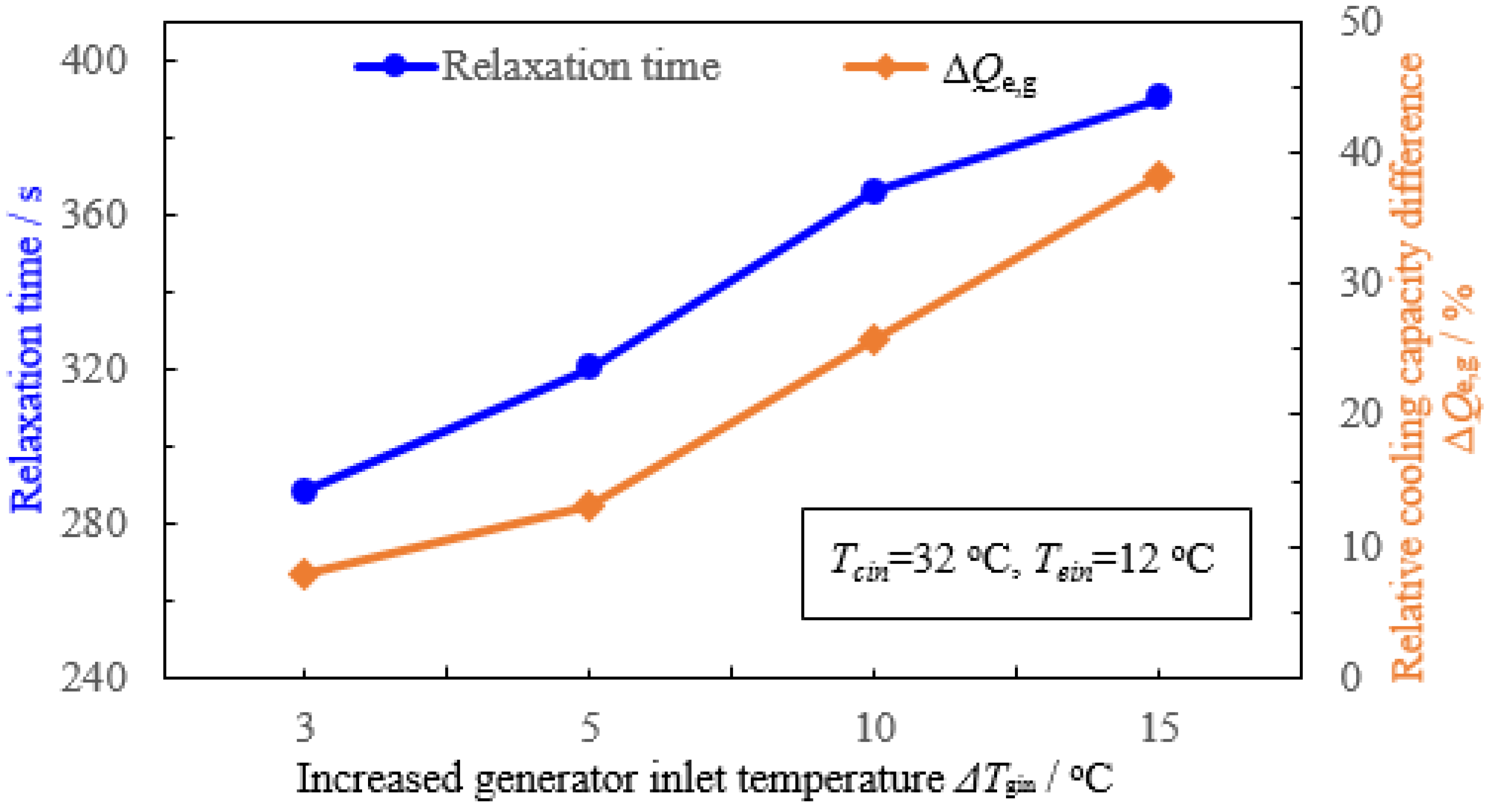
The former analysis is just with one step change of Tgin, Figure 6, Figure 7 and Figure 8 demonstrate the effects of different ΔTgin, which means the generator inlet temperature suddenly becomes 93, 95, 100 or 105 °C from 90 °C at time 0. Meanwhile, the cooling water inlet temperature Tcin and the evaporator inlet temperature Tein still keep at 32 °C and 12 °C, respectively.
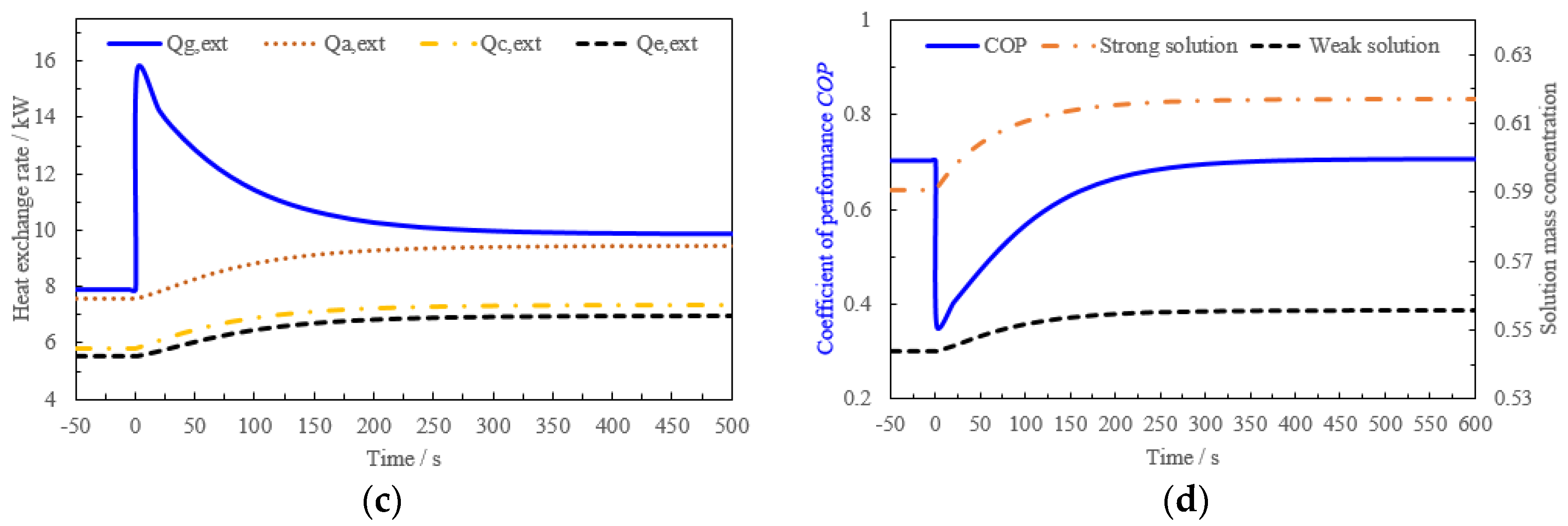
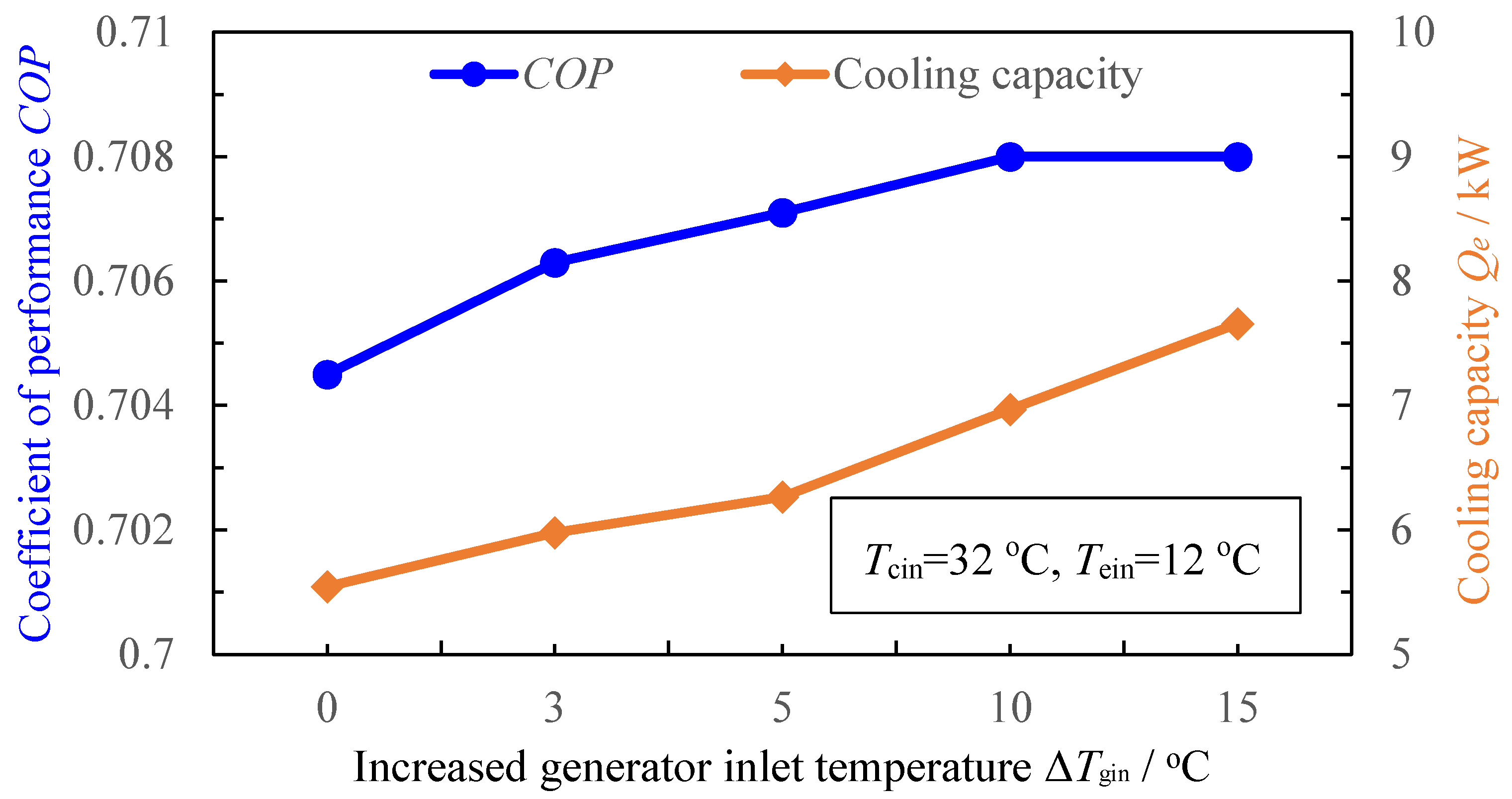
In Figure 6, the COP and the cooling capacity in steady-state becomes high when the generator inlet temperature increases, because the refrigerant mass flow rate in the cycle grows. Besides, the dynamic responses of the cooling capacities under different ΔTgin are demonstrated in Figure 7, showing that the time reaching a new steady-state is later when ΔTgin is higher. When ΔTgin becomes from 5 °C to 15 °C, the time increases 11.11–35.42% compared with ΔTgin = 3 °C. According to Equation (31), this means the relaxation time is longer, since the relative increment of the cooing capacity ΔQe,g is larger, as shown in Figure 8. And ΔQe,g is calculated with the data from Figure 6:
where Qe,(90+ΔTgin) is the cooling capacity in steady-state when the generator inlet temperature is 90 + ΔTgin, kW; Qe,90 is the cooling capacity in steady-state when the generator inlet temperature is 90 °C, kW.
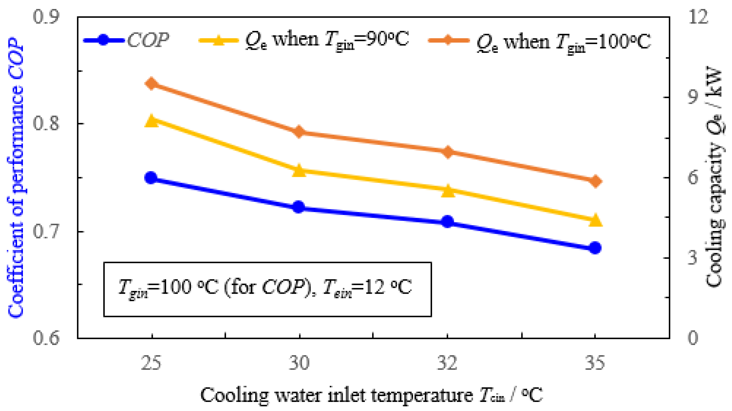
4.2. Different Cooling Water Inlet Temperature (Tcin)
Figure 9 displays the effect of different Tcin on the COP when Tgin = 100 °C and on the cooling capacities when Tgin = 90 °C or 100 °C, the evaporator inlet temperature Tein is 18 °C. These values come from steady-state model. The rise of Tcin leads to the increase of the generation pressure and the absorption temperature, restraining the generation and absorption processes, thus the COP and cooling capacities decrease.
When the generator inlet temperature always has a step change from 90 °C to 100 °C at time 0 and the evaporator inlet temperature Tein is 12 °C, Figure 10 shows the relaxation time and ΔQe under different Tcin. And the relative cooling capacity difference ΔQe is obtained with the data in Figure 9:
where Qe,100 and Qe,90 are the cooling capacities in steady-state when Tgin = 100 °C and Tgin = 90 °C, respectively, kW.
Although the cooling capacity in steady-state decreases with the increase of the Tcin, its relative variation ΔQe grows at the same time in Figure 10. Thus, the absorption chiller needs more time to achieve the next steady-state, the relaxation time increases by 5.65% when Tcin rises from 25 °C to 35 °C.
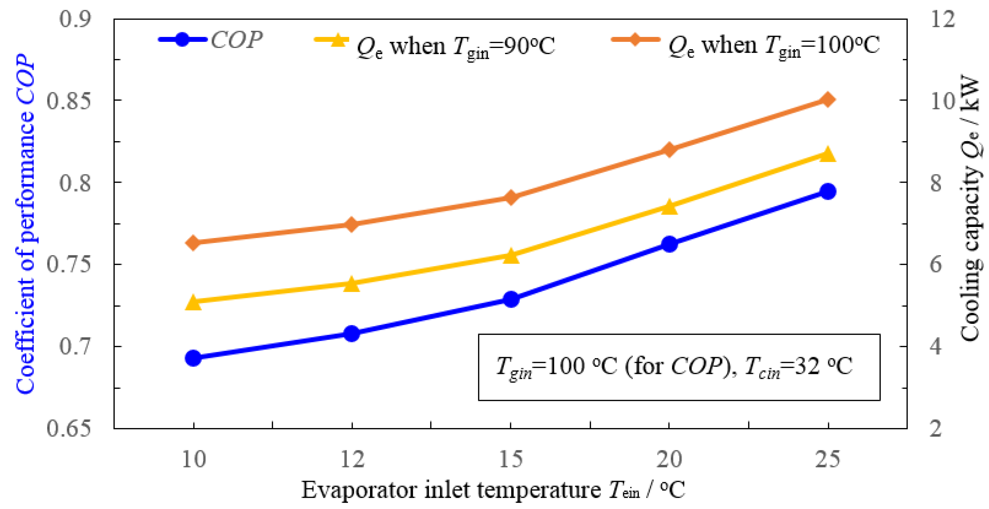
4.3. Different Evaporator Inlet Temperature (Tein)
Figure 11 displays the effect of different Tein on the COP when Tgin = 100 °C and on the cooling capacities when Tgin = 90 °C or 100 °C. The cooling water inlet temperature Tcin is 32 °C and the results are calculated by the steady-state model. Higher Tein is beneficial to the absorption process, so the COP and cooling capacities increase with the rise of Tein.
Figure 12 demonstrates the relaxation time and the relative cooling capacity difference ΔQe under different Tein, when the generator inlet temperature always has a step change from 90 °C to 100 °C at time 0 and the cooling water inlet temperature Tcin remains at 32 °C. The ΔQe increases with the decrease of Tein, as a consequence, the relaxation time rises by 3.95% when Tein reduces from 25 °C to 10 °C.
5. Application Analysis
To further clarify the application of the models, a whole system is built up. The AC is applied in a process plant used for raw material storage, whose temperature must be lower than 21 °C, otherwise the raw materials can decompose. The plant cooling load is simply calculated by:
where UAload is the product of the heat transfer coefficient and heat transfer area of the process plant, and is set as 0.3697 kW/K; Tout is the outdoor air temperature, °C; and Tin is the indoor temperature, °C.
And there is also thermal storage for the process plant:
where MCpload is the thermal capacity of the process plant, which is set to be 10 kJ/K.
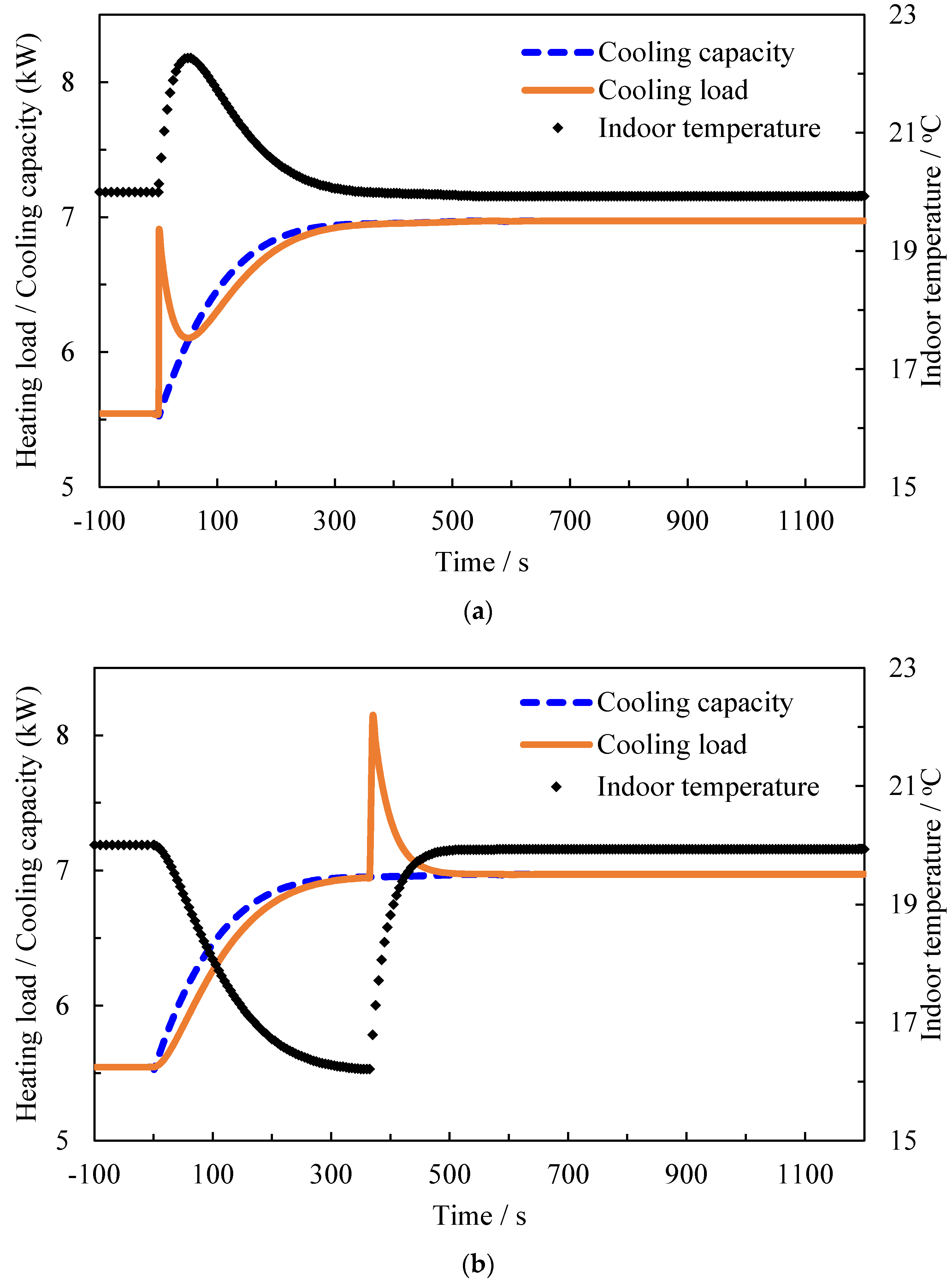
The outdoor temperature is 35 °C. The indoor temperature is 20 °C at the beginning, and the plant cooling load is 5.55 kW, but there will be some raw materials entering the process plant at a known time, which is expected to make the cooling load 1.4 kW higher. To meet the increased cooling demand, the AC cooling capacity is supposed to be increased accordingly. Based on Figure 7, the generator inlet temperature can grow from 90 °C to 100 °C when the cooling water inlet temperature Tcin and the evaporator inlet temperature Tein are 32 °C and 12 °C, respectively. In this study, two control methods are calculated, and the variations of the AC cooling capacity, indoor temperature and the plant cooling load are displayed in Figure 13a,b.
Figure 13a is adjusting the AC when the raw materials enter the process plant at time 0. The cooling load steeply becomes higher than the AC cooling capacity, which grows slowly, so the indoor temperature increases as high as 22.3 °C. Meanwhile, the outdoor temperature does not change, thus the cooling load reduces gradually. When the cooling load is lower than the AC cooling capacity, the indoor temperature starts to decrease, and the cooling load rises again until it equals to the AC cooling capacity. Finally, the indoor temperature reaches a new steady-state around 20 °C.
Variations of the AC cooling capacity, the indoor temperature and the plant cooling load are displayed in Figure 13b when the AC is adjusted 366 s earlier before these raw materials arrive, and this is the relaxation time according to Figure 8. The AC cooling capacity is higher than the plant cooling load after time 0, so the indoor temperature decreases, leading to the rise of the cooling load. When the time is 366 s, the cooling load has a 1.4 kW step change due to the new coming raw materials, as a consequence, the indoor temperature increases to near 20 °C, and then the plant cooling load decreases gradually until it becomes the same as the AC cooling capacity. In this dynamic process, the indoor temperature is always lower than 21 °C.
If the AC starts to be adjusted when the plant cooling load has a change, the indoor temperature can be higher than 21 °C in Figure 13a, while the indoor temperature cannot exceed the upper limit with early adjustment of AC. And in Figure 13b, the time starting to adjust can refer to the results in Part 4 when the working conditions are different. For example, the AC can start to change 354 s earlier when Tcin = 25 °C and Tein = 12 °C. These two control methods may be too simple, however, they demonstrate that the dynamic performance is beneficial for the adjustment of AC and the control of the whole system, which the AC belongs to. Thus, the AC transient process should be considered when the control strategy is made in the real practices.
6. Conclusions
Previous studies lack the dynamic performance of the absorption chiller (AC) under different working conditions, but it is significant for the operation of the whole system, of which the stabilization can be affected by the AC transient process. The steady-state and dynamic mathematical models of a single-effect absorption chiller are established in the present work, using the working fluids are H2O-LiBr. The dynamic model is applied to demonstrate the transient response to a 10 °C step change of the generator inlet temperature. Besides, the dynamic performance analyses are completed under different generator inlet temperatures, cooling water inlet temperatures and evaporator inlet temperatures. Furthermore, a whole system using AC in a process plant is analyzed. As a consequence, some conclusions can be drawn:
- (1)
- Compared with the step change of the generator inlet temperature ΔTgin = 3 °C, the time required to reach a new steady-state (relaxation time) increases by 11.11%–35.42% when ΔTgin increases from 5 °C to 15 °C.
- (2)
- The relaxation time grows with the rise of the cooling water inlet temperature Tcin, and it increases by 5.65% when Tcin changes from 25 °C to 35 °C.
- (3)
- Reducing evaporator inlet temperature Tein can lengthen the relaxation time, which rises by 3.95% when Tein decreases from 25 °C to 10 °C.
- (4)
- The control strategy considering the AC dynamic performance under different working conditions is beneficial for the real-time operation and control of the whole system.
Acknowledgments
The authors gratefully acknowledge the support of National Key Research and Development Program of China (No. 2016YFB0901405).
Author Contributions
Wenxing Shi, Xianting Li and Baolong Wang provided the guidance and revised the paper. Jian Wang, Sheng Shang and Wei Wu made the calculation.
Conflicts of Interest
The authors declare no conflict of interest.
Nomenclature
| A | bottom area, m2 |
| Cd | discharge coefficient |
| Cp | specific heat, kJ/(kg·K) |
| g | gravitational acceleration, m/s2 |
| H | vertical distance, m |
| h | specific enthalpy, kJ/kg |
| i | time, s |
| M | mass storage, kg |
| MCp | product of thermal storage mass and its specific heat, kJ/K |
| m | mass flow rate, kg/s |
| p | pressure, Pa |
| Pa | state parameters |
| Q | heat exchange rate, kW |
| S | section area, m2 |
| T | temperature, °C |
| V | volume, m3 |
| Vol | volumetric flow rate, m3/h |
| x | mass concentration of LiBr |
| UA | product of heat transfer coefficient and area, kW/K |
| z | fluid storage height, m |
| Greek symbols | |
| ρ | density, kg/m3 |
| ζ | resistance coefficient |
| ΔTgin | increased generator inlet temperature, °C |
| ΔQ | relative heat exchange rate difference, % |
| Abbreviations | |
| AC | absorption chiller |
| COP | coefficient of performance |
| LMTD | logarithmic mean temperature difference, °C |
| Subscripts | |
| a | absorber |
| c | condenser |
| con | container |
| e | evaporator |
| ext | external |
| des | desorbed refrigerant |
| g | generator |
| hx | heat exchanger |
| i | time |
| int | internal |
| l | refrigerant liquid |
| load | process plant |
| out | outlet |
| ref | reference |
| s | strong solution |
| st | steady-state |
| v | vapor |
| w | weak solution |
| wa | water |
| 1, 2···19 | points |
References
- Tsinghua University Building Energy Saving Research Center. 2009 Annual Report on China Building Energy Efficiency; China Architecture and Building Press: Beijing, China, 2009. (In Chinese) [Google Scholar]
- Ding, G.L. Recent developments in simulation techniques for vapour-compression refrigeration systems. Int. J. Refrig. 2007, 30, 1119–1133. [Google Scholar] [CrossRef]
- Wang, Q.; He, W.; Liu, Y.; Liang, G.; Li, J.; Han, X.; Chen, G. Vapor compression multifunctional heat pumps in China: A review of configurations and operational modes. Renew. Sustain. Energy Rev. 2012, 16, 6522–6538. [Google Scholar] [CrossRef]
- Wu, W.; Shi, W.X.; Li, X.T.; Wang, B.L. Air source absorption heat pump in district heating: Applicability analysis and improvement options. Energy Convers. Manag. 2015, 96, 197–207. [Google Scholar] [CrossRef]
- Lubis, A.; Jeong, J.; Saito, K.; Giannetti, N.; Yabase, H.; Alhamid, M.I. Solar-assisted single-double-effect absorption chiller for use in Asian tropical climates. Renew. Energy 2016, 99, 825–835. [Google Scholar] [CrossRef]
- Wu, W.; Wang, B.L.; Shang, S.; Shi, W.X.; Li, X.T. Experimental investigation on NH3-H2O compression-assisted absorption heat pump (CAHP) for low temperature heating in colder conditions. Int. J. Refrig. 2016, 67, 109–124. [Google Scholar] [CrossRef]
- Wang, J.; Wang, B.L.; Wu, W.; Li, X.T.; Shi, W.X. Performance analysis of an absorption-compression hybrid refrigeration system recovering condensation heat for generation. Appl. Therm. Eng. 2016, 108, 54–65. [Google Scholar] [CrossRef]
- Grossman, G.; Zaltash, A. ABSIM-modular simulation of advanced absorption systems. Int. J. Refrig. 2001, 24, 531–543. [Google Scholar] [CrossRef]
- Monné, C.; Alonso, S.; Palacín, F.; Serra, L. Monitoring and simulation of an existing solar powered absorption cooling system in Zaragoza (Spain). Appl. Therm. Eng. 2011, 31, 28–35. [Google Scholar] [CrossRef]
- Somers, C.; Mortazavi, A.; Hwang, Y.; Radermacher, R.; Rodgers, P.; Al-Hashimi, S. Modeling water/lithium bromide absorption chillers in ASPEN Plus. Appl. Energy 2011, 88, 4197–4205. [Google Scholar] [CrossRef]
- Ali, A.H.H.; Noeres, P.; Pollerberg, C. Performance assessment of an integrated free cooling and solar powered single-effect lithium bromide-water absorption chiller. Sol. Energy 2008, 82, 1021–1030. [Google Scholar] [CrossRef]
- Gutiérrez-Urueta, G.; Rodríguez, P.; Ziegler, F.; Lecuona, A.; Rodríguez-Hidalgo, M.D.C. Extension of the characteristic equation to absorption chillers with adiabatic absorbers. Int. J. Refrig. 2012, 35, 709–718. [Google Scholar] [CrossRef] [Green Version]
- Zamora, M.; Bourouis, M.; Coronas, A.; Vallès, M. Part-load characteristics of a new ammonia/lithium nitrate absorption chiller. Int. J. Refrig. 2015, 56, 43–51. [Google Scholar] [CrossRef]
- Wu, W.; Shi, W.; Wang, J.; Wang, B.L.; Li, X.T. Experimental investigation on NH3-H2O compression-assisted absorption heat pump (CAHP) for low temperature heating under lower driving sources. Appl. Energy 2016, 176, 258–271. [Google Scholar] [CrossRef]
- Ochoa, A.A.V.; Dutra, J.C.C.; Henríquez, J.R.G.; Dos Santos, C.A.C. Dynamic study of a single effect absorption chiller using the pair LiBr/H2O. Energy Convers. Manag. 2016, 108, 30–42. [Google Scholar] [CrossRef]
- Kohlenbach, P.; Ziegler, F. A dynamic simulation model for transient absorption chiller performance. Part I: The model. Int. J. Refrig. 2008, 31, 217–225. [Google Scholar] [CrossRef]
- Shin, Y.; Seo, J.A.; Cho, H.W.; Nam, S.C.; Jeong, J.H. Simulation of dynamics and control of a double-effect LiBr-H2O absorption chiller. Appl. Therm. Eng. 2009, 29, 2718–2725. [Google Scholar] [CrossRef]
- Kim, B.; Park, J. Dynamic simulation of a single-effect ammonia-water absorption chiller. Int. J. Refrig. 2007, 30, 535–545. [Google Scholar] [CrossRef]
- Cai, W.; Sen, M.; Paolucci, S. Dynamic modeling of an absorption refrigeration system using ionic liquids. In Proceedings of the ASME 2007 International Mechanical Engineering Congress and Exposition, Seattle, WA, USA, 11–15 November 2007; pp. 227–236. [Google Scholar]
- De la Calle, A.; Roca, L.; Bonilla, J.; Palenzuela, P. Dynamic modeling and simulation of a double-effect absorption heat pump. Int. J. Refrig. 2016, 72, 171–191. [Google Scholar] [CrossRef]
- Mansouri, R.; Bourouis, M.; Bellagi, A. Experimental investigations and modelling of a small capacity diffusion-absorption chiller in dynamic mode. Appl. Therm. Eng. 2017, 113, 653–662. [Google Scholar] [CrossRef]
- Myat, A.; Thu, K.; Kim, Y.D.; Chakraborty, A.; Chun, W.G.; Ng, K.C. A second law analysis and entropy generation minimization of an absorption chiller. Appl. Therm. Eng. 2011, 31, 2405–2413. [Google Scholar] [CrossRef]
- Butz, D.; Stephan, K. Dynamic behavior of an absorption heat pump. Int. J. Refrig. 1989, 12, 204–212. [Google Scholar] [CrossRef]
- Jeong, S.; Kang, B.H.; Karng, S.W. Dynamic simulation of an absorption heat pump for recovering low grade waste heat. Appl. Therm. Eng. 1998, 18, 1–12. [Google Scholar] [CrossRef]
- Kohlenbach, P.; Ziegler, F. A dynamic simulation model for transient absorption chiller performance. Part II: Numerical results and experimental verification. Int. J. Refrig. 2008, 31, 226–233. [Google Scholar] [CrossRef]
- Evola, G.; Le Pierrès, N.; Boudehenn, F.; Papillon, P. Proposal and validation of a model for the dynamic simulation of a solar-assisted single-stage LiBr/water absorption chiller. Int. J. Refrig. 2013, 36, 1015–1028. [Google Scholar] [CrossRef]
- Ochoa, A.A.V.; Dutra, J.C.C.; Henríquez, J.R.G.; Dos Santos, C.A.C.; Rohatgi, J. The influence of the overall heat transfer coefficients in the dynamic behavior of a single effect absorption chiller using the pair LiBr/H2O. Energy Convers. Manag. 2017, 136, 270–282. [Google Scholar] [CrossRef]
- Yin, H.; Qu, M.; Archer, D.H. Model based experimental performance analysis of a microscale LiBr-H2O steam-driven double-effect absorption Chiller. Appl. Therm. Eng. 2010, 30, 1741–1750. [Google Scholar] [CrossRef]
- Iranmanesh, A.; Mehrabian, M.A. Dynamic simulation of a single-effect LiBr-H2O absorption refrigeration cycle considering the effects of thermal masses. Energy Build. 2013, 60, 47–59. [Google Scholar] [CrossRef]
Figure 1.
The schematic of single-effect absorption chiller.
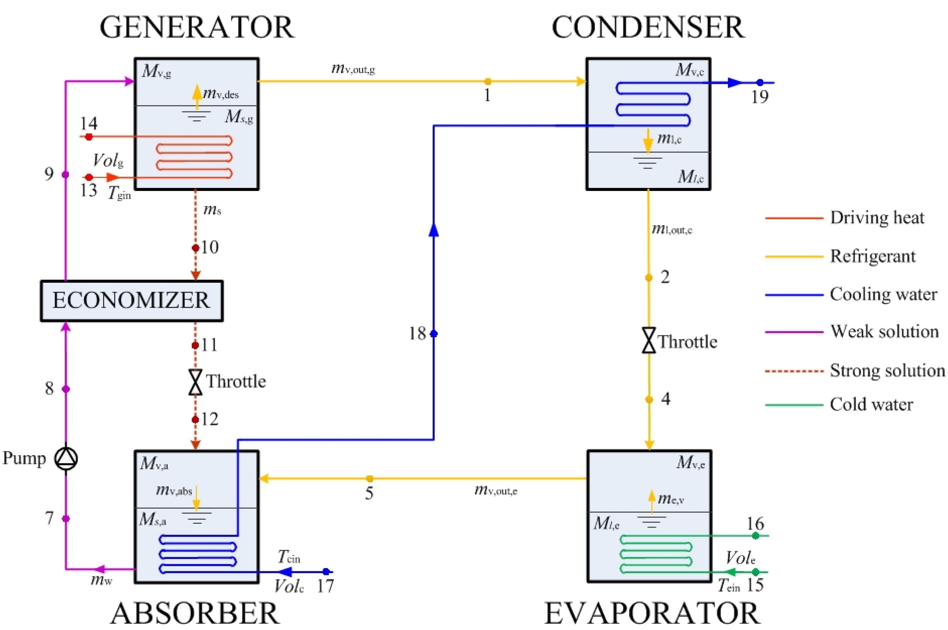
Figure 2.
The energy flow diagram in the generator; LMTDext,g: external logarithmic mean temperature difference in the generator.
Figure 2.
The energy flow diagram in the generator; LMTDext,g: external logarithmic mean temperature difference in the generator.

Figure 3.
The energy flow diagram in the condenser.

Figure 4.
Comparison between the model and the experiment; COP: coefficient of performance.

Figure 5.
Dynamic response to 10 °C step change of Tgin (Tcin = 32 °C, Tein = 12 °C); (a) The temperatures in the generator; (b) The mass flow rate. M; (c) The external heat exchange rates; (d) The COP and solution concentrations.
Figure 5.
Dynamic response to 10 °C step change of Tgin (Tcin = 32 °C, Tein = 12 °C); (a) The temperatures in the generator; (b) The mass flow rate. M; (c) The external heat exchange rates; (d) The COP and solution concentrations.


Figure 6.
The effect of different ΔTgin on the COP and cooling capacity.

Figure 7.
The dynamic responses of the cooling capacities under different ΔTgin.

Figure 8.
The effect of different ΔTgin on the relaxation time and ΔQe,g.

Figure 9.
The effect of different Tcin on the COP and cooling capacity.

Figure 10.
The effect of different Tcin on the relaxation time and ΔQe.
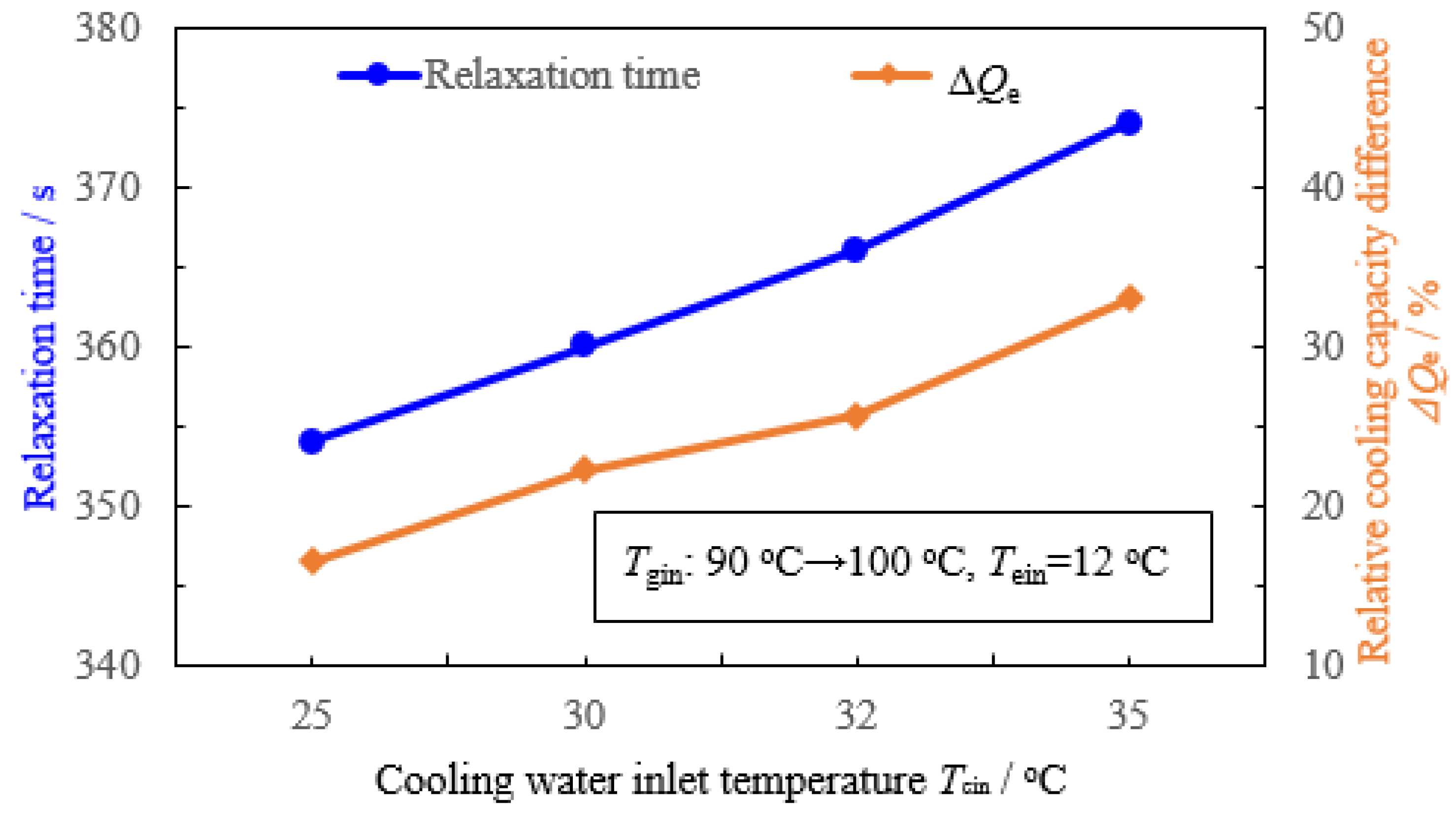
Figure 11.
The effect of different Tein on the COP and cooling capacity.

Figure 12.
The effect of different Tein on the relaxation time and ΔQe.
Figure 13.
Variations of AC cooling capacity, indoor temperature and plant cooling load; (a) Adjusting AC when raw materials enters the plant; (b) Adjusting AC before raw materials enters the plant; AC: absorption chiller.
Figure 13.
Variations of AC cooling capacity, indoor temperature and plant cooling load; (a) Adjusting AC when raw materials enters the plant; (b) Adjusting AC before raw materials enters the plant; AC: absorption chiller.

Table 1.
Constant parameters for the absorption chiller dynamic model.
| Parameter | Unit | Value | Parameter | Unit | Value |
|---|---|---|---|---|---|
| Ac | m2 | 0.10 | Sg | m2 | 0.0002 |
| Ag | m2 | 0.16 | UAext,a | kW/K | 4.78 |
| Cd | / | 0.61 | UAext,c | kW/K | 9.32 |
| Cpwa | kJ/(kg·K) | 4.19 | UAext,e | kW/K | 4.24 |
| g | m2/s | 9.81 | UAext,g | kW/K | 2.39 |
| Hc | m | 0 | UAint,a | kW/K | 5.97 |
| Hg | m | 0 | UAint,c | kW/K | 9.72 |
| MCpa,con | kJ/K | 58.31 | UAint,e | kW/K | 4.62 |
| MCpc,con | kJ/K | 32.82 | UAint,g | kW/K | 1.79 |
| MCpe,con | kJ/K | 37.83 | UAxs | kW/K | 0.042 |
| MCpg,con | kJ/K | 58.31 | Va | m3 | 0.024 |
| MCphx,a | kJ/K | 4.94 | Vc | m3 | 0.014 |
| MCphx,c | kJ/K | 3.04 | Ve | m3 | 0.024 |
| MCphx,e | kJ/K | 2.66 | Vg | m3 | 0.024 |
| MCphx,g | kJ/K | 2.66 | Volc | m3/h | 2.2 |
| Ml,c,0 | kg | 0.04 | Vole | m3/h | 1.34 |
| Ms,a,0 | kg | 0.09 | Volg | m3/h | 0.82 |
| Sc | m2 | 0.00002 | Volw | m3/h | 0.0666 |
© 2017 by the authors. Licensee MDPI, Basel, Switzerland. This article is an open access article distributed under the terms and conditions of the Creative Commons Attribution (CC BY) license (http://creativecommons.org/licenses/by/4.0/).
Share and Cite
MDPI and ACS Style
Wang, J.; Shang, S.; Li, X.; Wang, B.; Wu, W.; Shi, W. Dynamic Performance Analysis for an Absorption Chiller under Different Working Conditions. Appl. Sci. 2017, 7, 797. https://doi.org/10.3390/app7080797
AMA Style
Wang J, Shang S, Li X, Wang B, Wu W, Shi W. Dynamic Performance Analysis for an Absorption Chiller under Different Working Conditions. Applied Sciences. 2017; 7(8):797. https://doi.org/10.3390/app7080797
Chicago/Turabian StyleWang, Jian, Sheng Shang, Xianting Li, Baolong Wang, Wei Wu, and Wenxing Shi. 2017. "Dynamic Performance Analysis for an Absorption Chiller under Different Working Conditions" Applied Sciences 7, no. 8: 797. https://doi.org/10.3390/app7080797
Note that from the first issue of 2016, this journal uses article numbers instead of page numbers. See further details here.