Optimal Control of Wastewater Treatment Plants Using Economic-Oriented Model Predictive Dynamic Strategies


1
Department of Computing and automation, University of Salamanca, 37008 Salamanca, Spain
2
Department of Telecommunications and Systems Engineering School of Engineering, Universitat Autònoma de Barcelona, 08193 Catalonia, Spain
*
Author to whom correspondence should be addressed.
Appl. Sci. 2017, 7(8), 813; https://doi.org/10.3390/app7080813
Submission received: 1 July 2017
/
Revised: 25 July 2017
/
Accepted: 1 August 2017
/
Published: 9 August 2017
Abstract
:This paper addresses the implementation of economic-oriented model predictive controllers for the dynamic real-time optimization of the operation of wastewater treatment plants (WWTP). Both the economic-optimizing controller (pure-EMPC) and the economic-oriented tracking controller (Hybrid-EMPC, or HEMPC) formulations are validated in the benchmark simulation model (BSM1) platform that represents the behavior of a characteristic activated sludge process. The objective of the controllers is to ensure the appropriate operation of the plant, while minimizing the energy consumption and the fines for violations of the limits of the ammonia concentration in the effluent along the full operating period. A non-linear reduced model of the activated sludge process is used for predictions to obtain a reasonable computing effort, and techniques to deal with model-plant mismatch are incorporated in the controller algorithm. Different designs and structures are compared in terms of process performance and energy costs, which show that the implementation of the proposed control technique can produce significant economic and environmental benefits, depending on the desired performance criteria.
1. Introduction
In the management of a wastewater treatment plant (WWTP) operation, one of the most important factors that determines economics is the energy used to provide oxygen to the aerobic processes (aeration energy), and the pumping energy for the recycles of the plant. The appropriate adjustment of the available manipulated variables is crucial for an optimum operation, especially in the activated sludge process, where biological removal of nutrients and organic matter takes place [1,2,3].
The influent of the wastewater treatment plants exhibits an oscillating behavior, with daily and seasonal patterns associated with the human activities during the day and the seasonal rainfall. Weather conditions, such as rain and storms, produce significant changes in the influent flowrate and load [4]. Due to the variable influent behavior, the pollution load to be treated is continuously changing, and consequently, so are the energy and chemical requirements for the treatment. In such a scenario, conservative operation regulating the critical variables around the nominal working point might ignore the disturbances introduced by the influent. It is forecasted that significant energy savings could be achieved with an operation based on dynamic optimization that accounts for the influent conditions.
A detailed description of the developments of instrumentation and control systems for WWTPs can be found in Olsson [2]. Amand et al. [5] present a complete review of the aeration control strategies considering instrumentation, control algorithms, and even a description of the aeration system. They report that the most usual control solutions in the different WWTP control loops are based on simple proportional integral (PI) controllers. Even the derivative term is rarely used in practice [2]. These PI-based control loops (aeration, nitrate recirculation, cascade ammonia control, etc.) are usually based on regulation of the key variables at a constant set point. The benefits of advanced control techniques, such as model predictive control (MPC) for optimizing the operation of WWTPs, are pointed out in Santín et al. [3] and Amand et al. [5]; interesting applications are found in [6,7]. Due to the demand for solutions to improve the efficiency of WWTPs, particular attention is being paid to the application of real-time optimization systems (RTOs) [8,9,10,11,12]. The typical RTOs are hierarchical control structures that carry out the economic optimization of the set points in an upper level and send them the basic control level [13,14]. Recently, the single-layer economic model predictive control strategy has emerged as an alternative to the hierarchical RTO to perform the dynamic optimization of the operation improving the effluent quality and the economic performance [15,16].
The economic-oriented model predictive controller (EMPC) approaches include economic objectives in the cost function of the standard model predictive control (MPC) algorithm. It can be used as an optimizer in a hierarchical structure, or directly in the control level, combining the optimization and control tasks in the same algorithm [17]. The implementation directly in the control level is promising, since the algorithm is able to capture the impact of fast disturbances over plant behavior and process economics, thus providing the optimal control inputs, accounting for process restrictions [18]. Moreover, the use of single-layer structures reduces the computational effort, avoids communication problems between layers, and also avoids the use of different models in the optimization and control levels [13,19]. All of these characteristics make the single-layer EMPC an interesting solution to attain an adequate compromise between energy costs and effluent quality in the operation of WWTPs. The non-linear EMPCs have been successfully applied both in WWTPs in the upper layer of a hierarchical structure [8,9], and directly in the control level [15,16]. The non-linear models are appropriated despite their numerical complexity, because it is necessary to predict process behavior on a wide range of operating conditions. However, those applications use the exact process model for predictions of system behavior, which is an unrealistic assumption. In most cases, the model is not perfect, and it is necessary to deal with modeling errors that affect the controller performance.
In this work, a single-layer economic model predictive controller (EMPC) is proposed to perform the dynamic optimization of the operation of the activated sludge process of a WWTP. A standard simulation platform, the benchmark simulation model (BSM1), is used to test the two EMPC formulations, which are evaluated and compared in terms of the compromise between energy consumption and effluent quality achieved along the evaluation period. The economic-oriented controllers proposed in this work use an approximated non-linear phenomenological model of the process for predictions. The use of the simplified model reduces the computing effort on each controller execution, but produces plant-model mismatch problems while capturing its non-linear behavior. Here, the measurements of the constrained and the controlled variables are used to update the constraints and the cost function in the optimization problem, which is a technique commonly used to address plant–model mismatch problems that can produce infeasibilities and suboptimal operation [20].
Two formulations of the EMPC are considered in this paper, which are distinguished by the use of a pure economic cost function in the controller optimization problem, or a combination of a measure of the deviation from the set point and an economic performance index. The formulation of the economic performance indices is another important issue in the EMPC implementation. Here, the formulation is oriented to obtain a compromise solution between operating costs and effluent quality in terms of ammonium levels in the effluent. This trade-off is represented in the cost function by including an energy consumption index (economic terms) [21], and an index that quantifies the deviation from a desired legal value of the effluent ammonium concentration (quality term) [22].
A number of works addressing the implementation of single-layer EMCP approaches reflects its possibilities as an alternative to hierarchical RTO structures [17]. Nevertheless, its application to WWTPs is scarcely studied [15,16]. The goal of this paper is to show the suitability of the technique to minimize energy consumption and improve effluent quality by taking advantage of the dynamic behavior of the WWTPs. A novelty of the work with respect to previous works [8,15,16] is the execution of the optimization in a scenario where plant–model mismatch can affect the feasibility and the quality of the solution. Note that in the EMPC problem, the objective is the optimization of economics; then, the correction of the mismatch between the predictions and the measurements is quite different from set-point tracking problems [20].
2. Materials and Methods
This section presents the three elements involved in the proposed control problem. First of all, the considered economic model predictive control strategies are presented. These strategies are followed by the process description, which presents the wastewater treatment plant layout and process model, as well as the WWTP control problem and performance indices, in order to evaluate the performance of the plant operation. In the third subsection, the method by which the predictive controllers are applied to the WWTP process is explained through describing how the manipulated and controlled variables are used to specify the economic predictive controllers’ cost functions.
2.1. Description of the Proposed Control Strategies
The economic-oriented model predictive controller is a modification of the standard model predictive controller (MPC) that introduces a measure of process profitability in the cost function. In this section, first, the standard non-linear MPC is described briefly. Second, a general formulation that integrates the two possibilities for the economic-oriented model predictive controllers considered in this paper is presented.
2.1.1. Non-Linear Model Predictive Controllers
The MPC is an advanced controller that provides the optimal action for set-point tracking and control movements by solving an optimization problem, usually with constraints. In the MPC algorithm, the vector of manipulated inputs u is computed periodically and applied to the process each certain time, named sampling time (τS), from the optimization of a control performance index considering constraints on inputs, outputs and states. The typical performance index (cost function) in the MPC is a quadratic penalization of the target (set point) deviations and the magnitudes of the manipulated inputs adjustments that represent the rate of variation of actuators. The set point can be a fixed value, or a computed value provided by an upper level optimization. A model of the process to be controlled is used to predict the future behavior, in a given time horizon τN [23].
Different types of models can be used for predictions in the MPC algorithm, e.g., linear or non-linear models expressed in discrete-time or in continuous-time [24]. In this work, a non-linear model of the system is selected, which is stated as a continuous time state-space model:
where is the state vector that contains the process variables that are relevant in the control problem, and X is the set of admissible states; is the vector of manipulated inputs, and U represents the physical limitations of the manipulated variables; is the vector of measured disturbances, and V is the set of measurable disturbances, and denotes the time derivative of the state. Note that only measurable disturbances are considered here.
2.1.2. Economic-Oriented Model Predictive Controllers
The economic-oriented model predictive controllers follow a similar strategy to the standard MPC controllers, but in this case, the cost function includes a term representing the economic performance, the energy savings, or a measure of process performance associated to the economic profit. There are several types of economic-oriented controllers with these characteristics [17], and in this work, the economic optimizing controller (pure-EMPC) and the economics-oriented tracking controller (Hybrid-EMPC or HEMPC) have been considered.
In the pure EMPC, the control actions are obtained considering a cost function that only includes this economic term, without any other tracking or control-movement terms. On the other hand, the economics-oriented tracking controller (HEMPC) cost function includes the economic term as well as the other terms explained in the previous section [25,26].
Note that the HEMPC is more appropriated in the cases where some output variables must be maintained around some reference values to ensure the desired process performance, while also allowing for some deviation from the set point. This deviation is tolerable when economic performance and the tracking of the reference are conflicting objectives or in contrast, the simultaneous optimization of economics and control performance is possible because additional degrees of freedom are available [26]. The tuning parameters have to be carefully selected to find an appropriated compromise solution.
A generalized mathematical description that includes both alternatives is presented here.
subject to:
JECO in (Equation (2)) is an economic performance index measuring the operating profits or expenses, and JNMPC is the MPC cost function described in the previous section. The relative importance of the objectives in the cost function is given by the weights wC and wE. They have to be carefully selected to represent the desired compromise between economics and control performance. The constraints and initial conditions are defined by Equations (2a)–(2c). Since both objectives are represented as separate terms, the problem described results in a conventional MPC formulation when the weight wE is set to zero (wE = 0, wC ≠ 0), and in an economic-optimizing controller or pure EMPC formulation, when wC is set to zero (wE ≠ 0, wC = 0). If wE ≠ 0, wC ≠ 0, then it is the case of an economic-oriented tracking controller or HEMPC, where the two terms have to be suitably weighted to represent the desired compromise between economics and control performance.
The decision variables in Equation (2) are the manipulated inputs u, which are generally defined as a trajectory along the prediction horizon u(t|τk). For each input trajectory u that the optimizer proposes (note that the optimization is solved iteratively), the predicted states and outputs y are obtained using the non-linear model (1). However, in the implementation of the controller in this work, the trajectory u(t|τk) is considered to be a constant value u for simplicity, and this will be the control action applied to the plant. Therefore, there is only one decision value in Equation (2), and the problem can be solved easily by Sequential Quadratic Programming methods (SQP). This assumption is analogous to the selection of a control horizon of 1 in a typical discrete MPC, because the control horizon is defined as the number of discrete changes allowed for the control signal during the prediction horizon before stabilizing. In any case, although the consideration of control horizons greater than 1 is straightforward through considering more decision variables in the optimization problem (representing step changes in the control signal during the prediction horizon time), it has not been implemented because it increases the computational times, and the improvement of the results is not remarkable.
As for predictions and other magnitudes in the cost function [17], although a continuous model is considered, a discrete update of the manipulated variable is performed because the optimization problem is solved at each sampling time τs. More precisely, the problem is solved at the time instants given by the sequence , where , and τk is the sampling time instance of the continuous time model. Therefore, each time the optimization problem (2) is solved, the increments of the manipulated variable are obtained considering u(τk−1) as starting value.
Finally, note that due to the use of a reduced model of the process for predictions, there is a plant–model mismatch that is tackled here by applying a bias correction [23]. More precisely, it consists of modifying the set point and output constraints using the difference between the measured output and predicted output at each sampling time. This correction is equivalent to a Dynamic Matrix Control (DMC) scheme that has been proved to be effective in these cases [23].
2.2. WWTP Process and Model Description
As the control problem statement used in this work is based on the use of a process model for prediction purposes, it is convenient to separately present both descriptions: first, the description of the WWTP process, based on the BSM1, and second, the simplified model used as the prediction model.
2.2.1. WWTP Process: BSM1
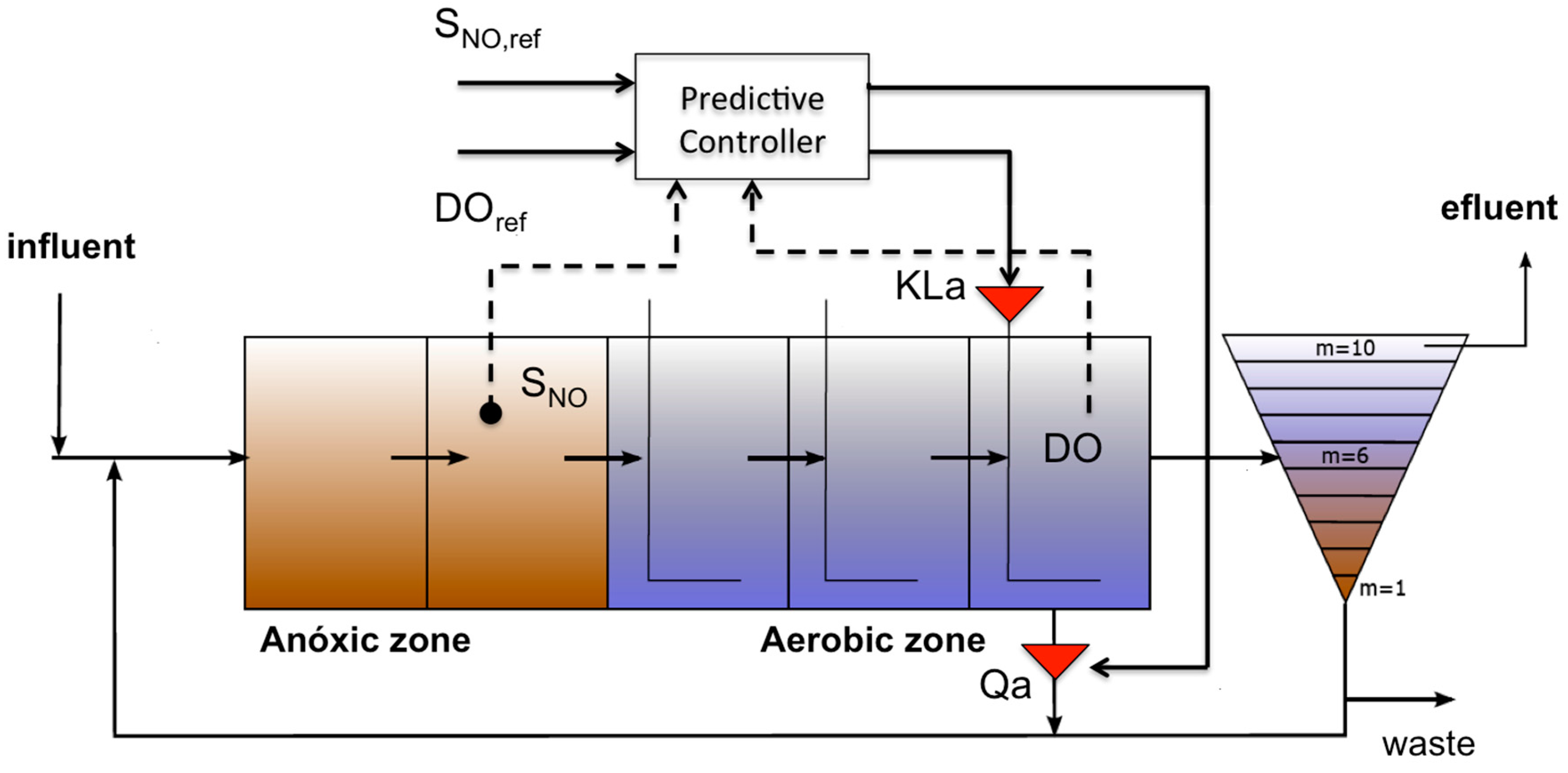
The benchmark simulation model 1 [21] is used to represent the activated sludge process in a WWTP. The simulation platform (Benchmark simulation model, or BSM1) has been developed within COST Actions 624 and 682. The schematic representation of the WWTP layout and default control strategy considered in BSM1 is presented in Figure 1. The plant consists of five biological reactor tanks connected in a series, followed by a secondary settler. The first two tanks have a volume of 1000 m3 each, and are anoxic and perfectly mixed. The remaining three tanks have a volume of 1333 m3 each, and are aerated. The settler has a total volume of 6000 m3, and is modeled in 10 layers, with the sixth layer when counting from bottom to top functioning as the feed layer. Two recycle flows, the first from the last tank, and the second from the underflow of the settler, complete the system. The sludge from the settler that is not recycled is led to be disposed, and is called wastage.
The plant is designed for an average influent dry weather flow rate of 18,446 m3/day and an average biodegradable chemical oxygen demand (COD) in the influent of 300 g/m3. Its hydraulic retention time, based on the average dry weather flow rate and the total tank and settler volume (12,000 m3), is 14.4 h. Qw is fixed to 385 m3/day, which determines, based on the total amount of biomass present in the system, a biomass sludge age of about nine days.
The nitrogen removal is achieved using a denitrification step performed in the anoxic tanks, and a nitrification step carried out in the aerated tanks. The internal recycle is used to supply the denitrification step with SNO. The biological phenomena of the reactors are simulated by using the Activated Sludge Process No1 (ASM1), which considers eight different biological processes. The double-exponential settling velocity model simulates the vertical transfers between layers in the settler [27]. No biological reaction is considered in the settler. The two models are internationally accepted and include 13 state variables [28]. The full mathematical model, the physical parameters and performance indices can be found in [22].
The default control strategy proposed in the BSM1 (Figure 1) consists of two PI loops: (1) control of the dissolved oxygen concentration in the fifth reactor (SO5) manipulating the oxygen transfer coefficient KLa5, and (2) control of the nitrates concentration in the anoxic zone (SNO2) manipulating the internal recycle flow rate Qa.
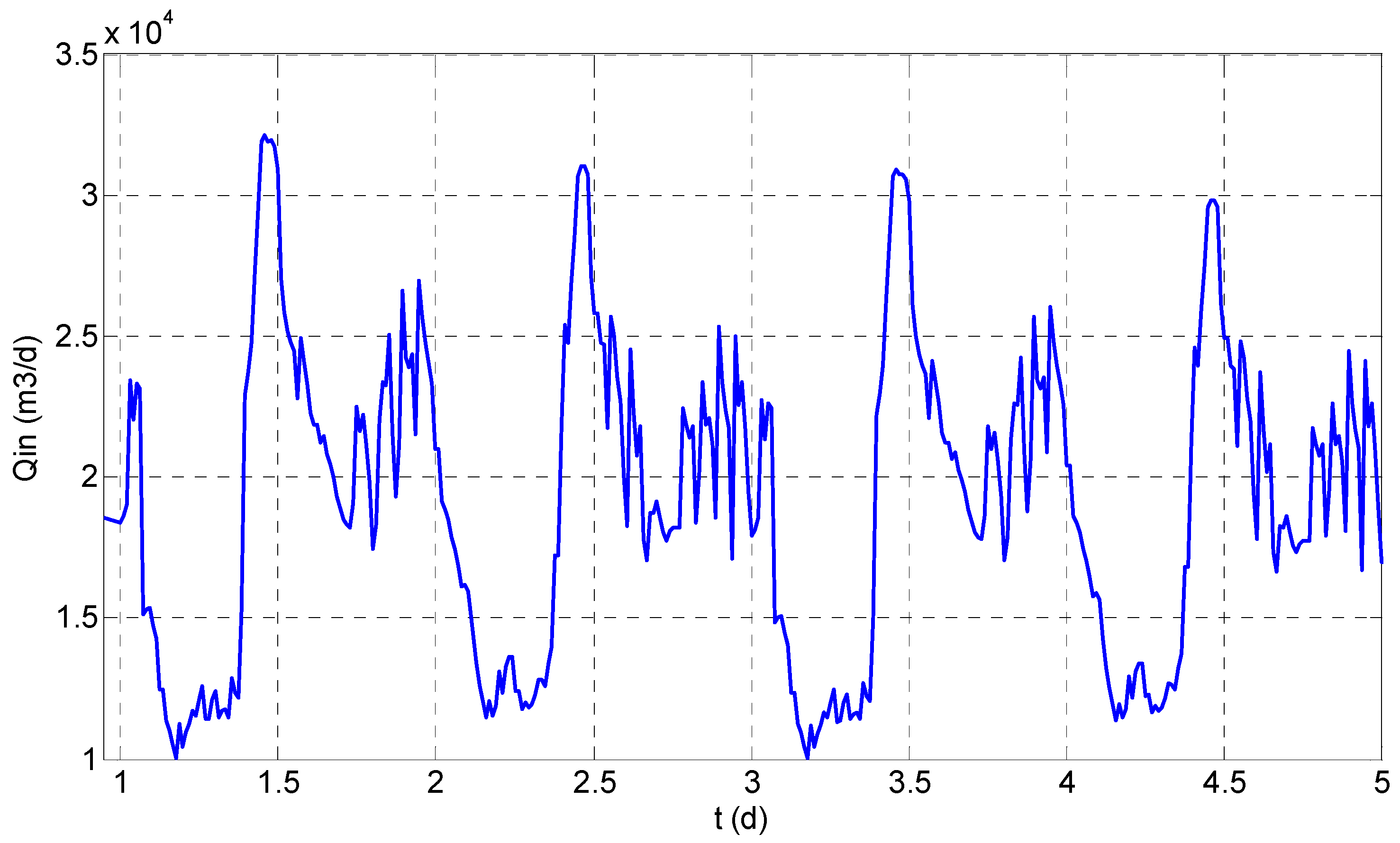
The BSM1 also provides different influent profiles depending on the weather conditions (dry, rainy, stormy) to evaluate the plant performance. For example, dry weather influent flow is shown in Figure 2.
2.2.2. WWTP Model for Prediction: Reduced BSM1
As told, the BSM1 uses the ASM1 to represent the behavior of the biological reactors. The use of the complete BSM1 as a non-linear model for prediction would suppose an excessive computational burden, as well as the unrealistic situation where the process is modeled perfectly and all the state variables are accessible. Therefore, in this work, it is proposed to use a reduced version of the BSM1 as the model for prediction [28]. This reduced model introduces simplifications at two levels: layout and biological processes.
Regarding the layout of the model, it is reduced to one anoxic reactor and one aerobic reactor with a volume equivalent to the anoxic and aerobic zones of the BSM1, respectively. The index i is used to distinguish the units, with reactor 1 being the anoxic zone (i = 1), and reactor 2 the aerobic zone (i = 2).
Concerning the biological processes, ASM1 uses 13 state variables on each reactor and considers eight biological processes. In the reduced model, only the faster biological processes are taken into account. The influent variables considered in the reduced model are: the influent flow (Qin), the organic matter concentration (SS,in), and the ammonium concentration (SNH,in). The manipulated variables are the oxygen transfer coefficient (KLa), and the internal recycle flow (Qa).
The equations of the reduced model, the list of the model parameters, and the variables considered in the reduced model used here are presented in Appendix A.
2.2.3. WWTP Control Problem
The control problem formulation is based on the influence of the activated sludge process variables on the general performance of the WWTP. The effluent quality is given by the limits imposed by the environmental regulation over nutrients and organic matter concentration of WWTP discharges. The effluent quality limits considered here are those defined within the BSM1 in [22] and reproduced here in Table 1.
The violations of the established limits over pollutants concentration in the effluent presented in Table 1 has an impact on economics due to the fines imposed for off-specification discharges. In the periods of lower load, the reduced levels of pollutants facilitate the treatment, and the effluent quality standards can be achieved even with values of dissolved oxygen (DO, also denoted by SO2) below the reference. The regulation of the dissolved oxygen concentration (SO2) and nitrates (SNO1) to reference values that ensure the desired process performance implies the use of energy for aeration and pumping purposes. In this situation, driving these variables to the set point using a conservative control strategy may result in unnecessary energy consumption. On the other hand, during the periods of higher load, it is necessary to increase the biological activity to reduce the excessive amount of pollutants. Then, the attainment of the set points for SO2 and SNO1 is decisive to meet the effluent quality specifications or minimize the violations of the imposed limits to avoid economic penalties.
The desired levels over COD in Table 1 are easily satisfied. The total nitrogen (TN) includes, among others, the NH4+ + NH3 compounds. These compounds are more damaging than nitrates in the effluent (SNO,e). Therefore, in this work, the effluent quality is measured considering only the concentration of NH4+ + NH3 compounds in the effluent (SNH,e). A concentration of NH4+ + NH3 compounds in the effluent below 4 mg/L is desired. A performance index that measures the economic penalty for violations of the SNH,e as a function of the concentration of ammonium compounds in the ASP (SNH) is [21]:
The index Cost_NHeff is a measure of the load in excess accumulated in the operating period. In practice, the bound of 4 mg/L is applied over the daily mean concentration of the NH4+ + NH3 compounds in the effluent (SNH,e).
In addition to the economic penalty for effluent limit violation, operating costs related to energy consumption are also considered. They include the aeration energy and the pumping energy, which are measured using the cost indices proposed in the BSM1 platform [22].
In this case study, the Pumping Energy (PE) represents the energy use for the pumping of internal recycle flow (Qa):
where t0 and tf are the initial and final times considered for the index evaluation and .
The oxygen transfer coefficient KLa is a parameter that takes into account factors such as the type of diffuser in the reactors, bubble size, and depth of submersion. The Aeration Energy (AE) is calculated from KLa according to the following equation:
The overall cost index (OCI) includes the pumping energy (PE) and the aeration energy (AE):
w1 and w2 are cost factors that provide an economic interpretation to the OCI; they are chosen here as w1 = w2 = 1 EUR/kWh.
2.3. Application of the Control Strategies to the WWTP
In the implementation of the controllers to the wastewater treatment plant represented by the BSM1 platform, it is necessary to translate the variables of the reduced model that consist of one anoxic reactor and one aerobic reactor, with a total volume equivalent to the two anoxic basins and the three aerobic basins of the BSM1 plant. Moreover, some considerations related to process characteristics and the model mismatch problem in the controller implementation must be clarified. These considerations, as well as the correspondence between the variables, performance indices and constraints handled by the proposed non-linear model predictive controller (NMPC) and economic-oriented MPC designs, and the BSM1 plant, are described below.
2.3.1. Control Problem Formulation
At each sampling time, the controller receives information from the plant and translates this information to the variables considered by the control algorithm.
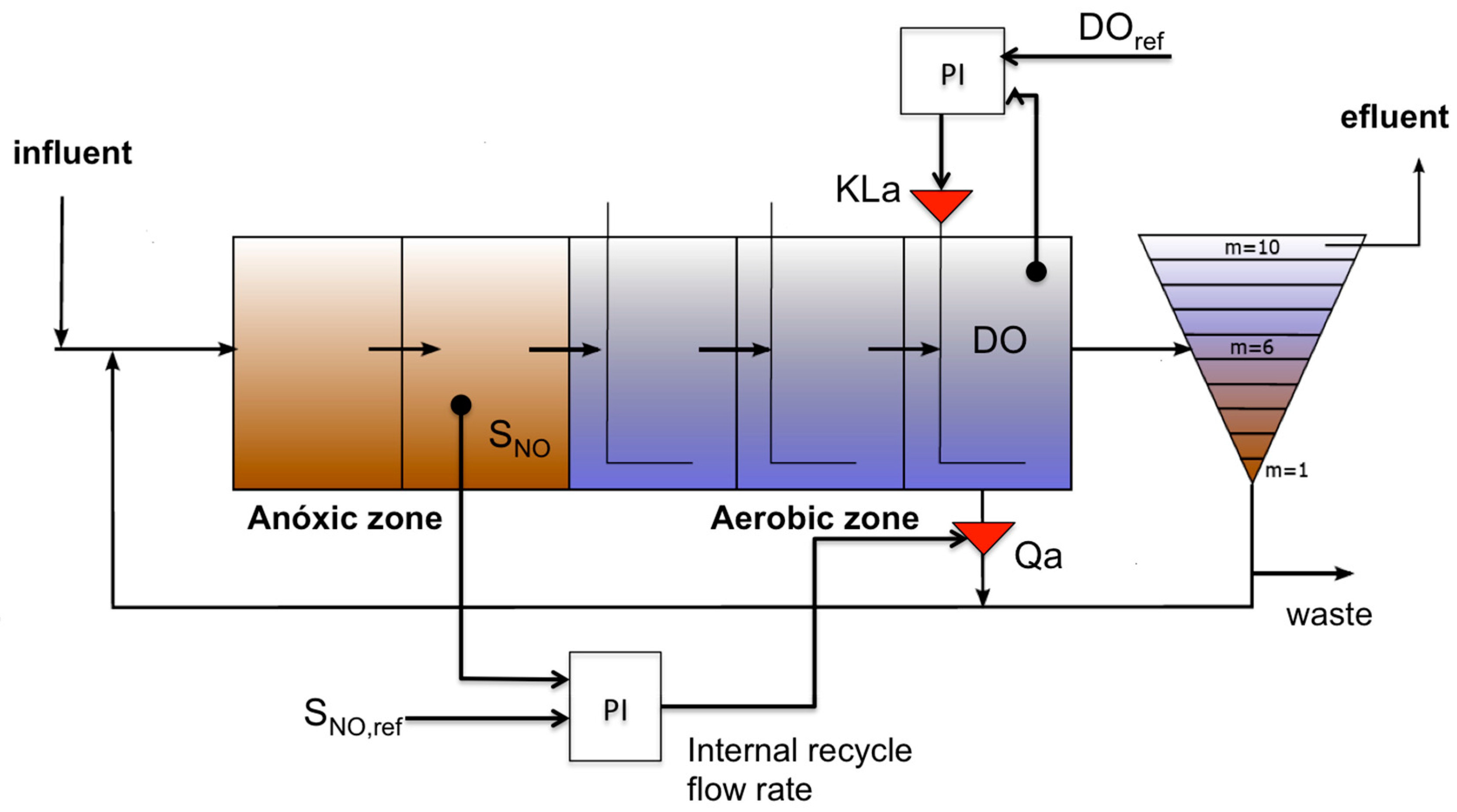
The non-linear process model described by Equations (A1)–(A11) is used as a prediction model (Equation (1) in Section 2). Then, the controller optimization problem is solved, taking into account the reduced model variables and the computed manipulated variables that are sent to the plant. Therefore, the control problems presented in Section 2 are written here in terms of the reduced model variables. A schematic representation of the proposed control strategy in the BSM1 plant is presented in Figure 3.
The formulation of the control problem in this work considers a multivariable strategy, where reference values of the nitrates concentration, SNO2_SP = 1 g/m3; and dissolved oxygen concentration, SO5_SP = 2 g/m3; are provided manually or by an upper level optimization for a long time-operating horizon. The manipulated variables are KLa and Qa.
Regarding the control variables, the control performance is expressed in terms of the vector of output variables and the set points .
Therefore, the MPC performance index includes only the predicted values of the controlled variables y(t), which are selected from the state vector x(t), and the manipulated inputs , considering that the control signal is constant along the prediction horizon.
Moreover, the controller only receives measurements of the influent variables that are considered in the reduced model and have a significant effect in the plant performance, which are the influent flow, ammonium concentration, and organic matter concentration.
Summarizing, the specific WWTP control problem variables considered in this application are:
- State vector:
- Output variables (controlled variables):
- Measured disturbances:
- Vector of manipulated inputs:
- Set points: SNO1_SP = 1 mg/L and SO2_SP = 2 mg/L
The control performance index is the following equation, which includes a term for set-point tracking error, control movements and a terminal penalization for set-point tracking:
where Wy is the weight matrix for the corresponding controlled states, Wu is a weight matrix for the control efforts, and Wn is a weight matrix for the terminal penalization. The operator is used to denote the square of a weighted Euclidean norm of a vector, where Q is a positive definite matrix.
The economic performance (JECO) is measured using the overall cost index (OCI) described by Equation (6), which includes the pumping energy, aeration energy and fines for off-specification ammonium concentration.
where, w1 = w2 = 1 EUR/kWh and Qe is the effluent flow.
The JECO index (EUR/day) represents the compromise between the energy consumption (OCI), weighted by w1 and computed as the sum of the pumping energy (first term) and the aeration energy (second term), and the fines for off-specification ammonium concentration in the effluent weighted by w2.
Process constraints are imposed over the manipulated variables KLa5 and Qa [22] and the controlled variables SNO2 and SO5, which are expressed according with the reduced model variables.
In some cases, under strong disturbances, it may not be possible for the plant to satisfy all the constraints. Then, Equations (11)–(13) are formulated as soft constraints. The constraints are imposed over the reduced model states in order to meet the effluent quality limits presented in Table 1. These values are selected from a preliminary study of the process behavior that allowed establishing an approximated relation between the effluent characteristics and the reduced model outputs.
2.3.2. Particular Characteristics of the Controllers Implementation
The first issue to address when implementing the proposed controllers to the BSM1 plant is the equivalence between the plant variables and the reduced model variables, and the model mismatch. It is assumed that the organic matter concentration, ammonium concentration, nitrates and nitrites concentration, and dissolved oxygen concentration in the second anoxic reactor and the fifth reactor, as well as the heterotrophic and autotrophic biomass concentration, are measurable variables. Then, these measurements are used to initially build the state vector for the reduced model, making the following equivalence:
- Second anoxic reactor measures --> ammonium concentration (SNH1), readily biodegradable substrate concentration (SS1), nitrates and nitrites concentration (SNO1), and dissolved oxygen concentration (SO1).
- Fifth aerobic reactor measures --> ammonium concentration (SNH2), organic matter concentration (SS2), nitrates and nitrites concentration (SNO2), and dissolved oxygen concentration (SO2).
The current values of the heterotrophic and autotrophic biomass concentration are used as constant parameters in the model. The set points for the reduced model are SNO1_SP = 1 mg/L and SO2_SP = 2 mg/L in the reduced model.
In order to deal with the plant–model mismatch problem (see Figure A1, Figure A2 and Figure A3), the difference between the BSM1 plant measurements and the reduced model outputs (denoted ei) is computed at each sampling time, and it is used for bias correction of the set points and constraints limits in the optimization problem described above (Equations (2)–(2c)). For instance, see the following constraint (13) modification, where the bound has been decreased by the difference between the plant measurement and the model output: .
Regarding the pure-EMPC implementation, performing an optimization of economic objectives to obtain the manipulated variables might lead the operation to the limits of the constraints in long time horizon, producing performance deterioration. In order to guarantee feasible solutions in the whole operating period, a first attempt of the optimization of the economic function is carried out, and if infeasibilities arise, a second optimization is executed using an HEMPC cost function (with a tracking term introduced to recover feasibility). This is a particular characteristic of the proposed pure EMPC, but all the controllers implemented in this paper use the manipulated variables values obtained in the previous sampling time when no feasible solutions are found in the current controller execution.
Regarding the HEMPC’s implementation, it is clear that this controller formulation has to deal with competing economics and control objectives, whose importance in the hybrid cost function is given by the weights wE and wC (Equation (2) with wE ≠ 0, wC ≠ 0). In order to maintain the controlled variables at the desired reference value, it is necessary to consume energy, which increases the operating costs. Then, the minimization of the pumping energy (PE) and aeration energy (AE) produce a deviation respect to the desired set points, since not enough freedom degrees are available to meet both requirements at the same time. This deviation is tolerated while the constraints required for the effluent quality are fulfilled.
2.4. Algorithmic Implementation and Simulation Settings
The full BSM1 benchmark simulation model implemented in Matlab/SIMULINK has been selected to test the controllers proposed. In the algorithmic implementation, the optimization problem is solved, with each sampling time using the sequential quadratic programming method given by the algorithm fmincon.
After some preliminary tests, the tuning parameters of the NMPC are adjusted. The prediction horizon is = 5 h, and the weights of the different objectives of the controllers cost are: , .
For all controllers, the sampling time selected is τ = 5 min, after some trial and error study of this parameter. Some simulations have been performed with τ = 3 min, but this change does not improve results and the computational time increases considerably. On the other hand, considering τ = 15 min, which is an increment of the sampling time, might lead the control system not to capture the process dynamics properly, such as nitrates stabilization after some influent disturbances affect the process, for example.
The weights wC for control objectives and wE for the economic objectives are selected according to the objectives of the different controllers. Then, wC = 0, wE = 1, for the pure-EMPC, and wC = 1, wE = 10 for the HEMPC.
Both formulations of the economic oriented controllers are validated with three different sets of weights of the economic cost function (Equation (8)): w1 = 1, w2 = 0 (EMPC-OCI/HEMPC-OCI); w1 = 0, w2 = 1(EMPC-NH/HEMPC-NH); and w1 = 1, w2 = 1 (EMPC-OCI + NH/HEMPC-OCI + NH), and compared with the traditional NMPC described in Section 2.1.
3. Simulation Results and Discussion
Several simulations are carried out to study the process behavior with the different controllers and their effect on process economics and removal efficiency. The performance indices provided by the BSM1 platform are used to evaluate the process performance, with the different controllers in the operating period under characteristic dry weather influent variations.
The evolution of the most relevant process variables along the operating horizon is presented in the following figures. First, the comparison between the standard NMPC, which is focused on the set-point tracking, and the HEMPC (HEMPC-OCI: w1 = 1, w2 = 0, HEMPC-NH: w1 = 0, w2 = 1) is presented. The controlled variables are shown in Figure 4, and the corresponding control signals (manipulated variables) are shown in Figure 5. The NMPC exhibits an acceptable set-point tracking even though an offset is observed, especially in the nitrates concentration (SNO2). Although better set-point tracking could be attained using more elaborated techniques to deal with the plant–model mismatch problem, it is not a critical issue because the objective of the proposed control strategies is to improve the economic aspects in the operation. In the operation under HEMPC-OCI, the SNO2 and SO5 responses present higher variation between the operational limits than the NMPC and HEMPC. The evolution of the control inputs with the different controllers is presented in Figure 5, where it is possible to see that the weights given to the economics in JECO (Equation (8)) in the controller algorithm significantly affect the control signal. The recycle flow (Qa) is especially affected, showing more intensive movements in the NMPC in order to reach the set point than in the hybrid controllers. In the case of the HEMPC-OCI, a lower recycle rate minimizes the pumping energy. In the case of HEMPC-NH, it could be interpreted in the sense that the lower values of the recycle are favorable for ammonium elimination. A similar trend is appreciated in the aeration energy, but in lower magnitude.
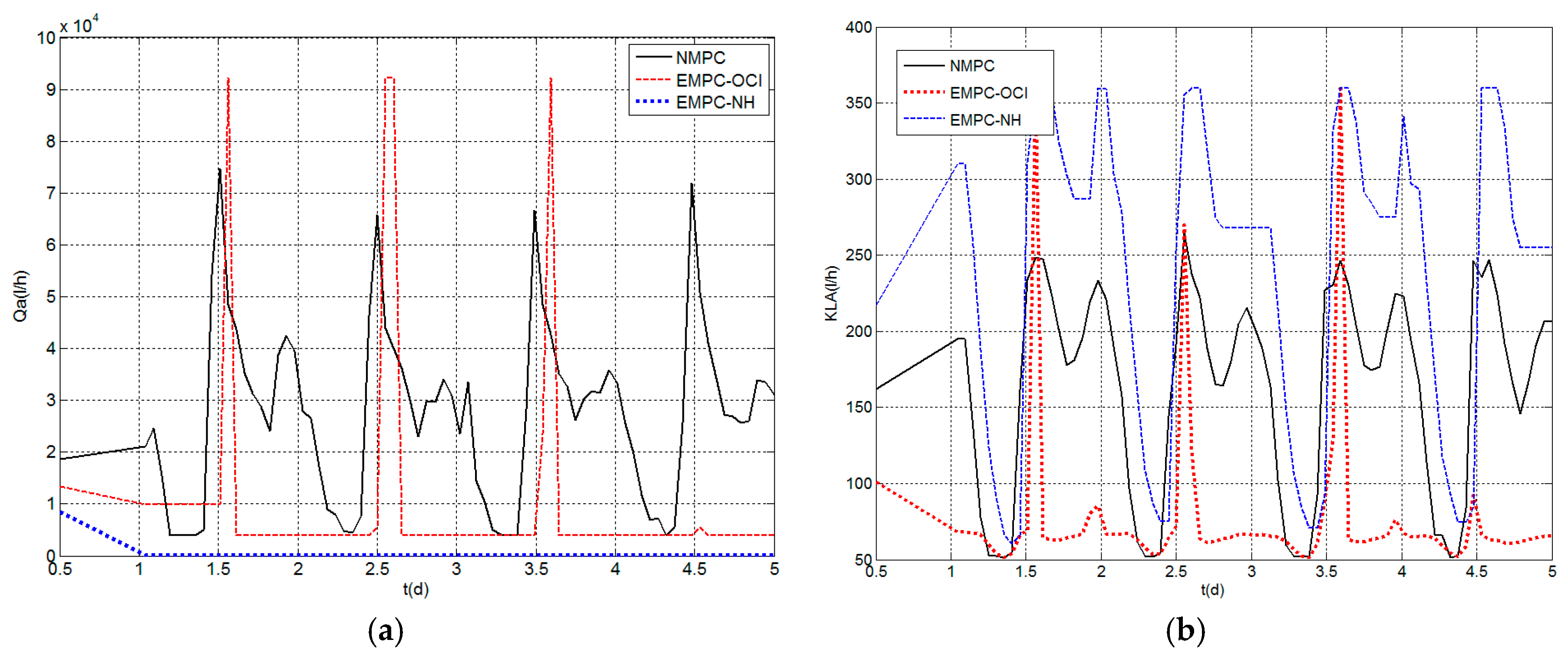
In the case of the pure-EMPCs (Figure 6 and Figure 7), the effect of the weighting of the energy costs and the penalization for off-specification ammonium concentration in the effluent in the economic cost function is more notorious than in the hybrid controllers, since the values of the manipulated variables are uniquely determined by the optimization of the economic performance index JECO. Then, significance differences can be observed in the response of the controlled variables when using each controller. Particularly, the oxygen concentration increases with the EMPC-NH to improve the ammonium elimination, and decreases with the EMPC-OCI due to the minimization of the aeration energy. The minimization of the pumping and aeration energy carried out by the EMPC-OCI produces lower values of both manipulated variables, as expected. On the other hand, it can be seen that the minimization of the off-specification ammonium concentration in the effluent performed by the HEMPC-NH requires more aeration (KLa), but minimum values of the recycle flow (Qa).
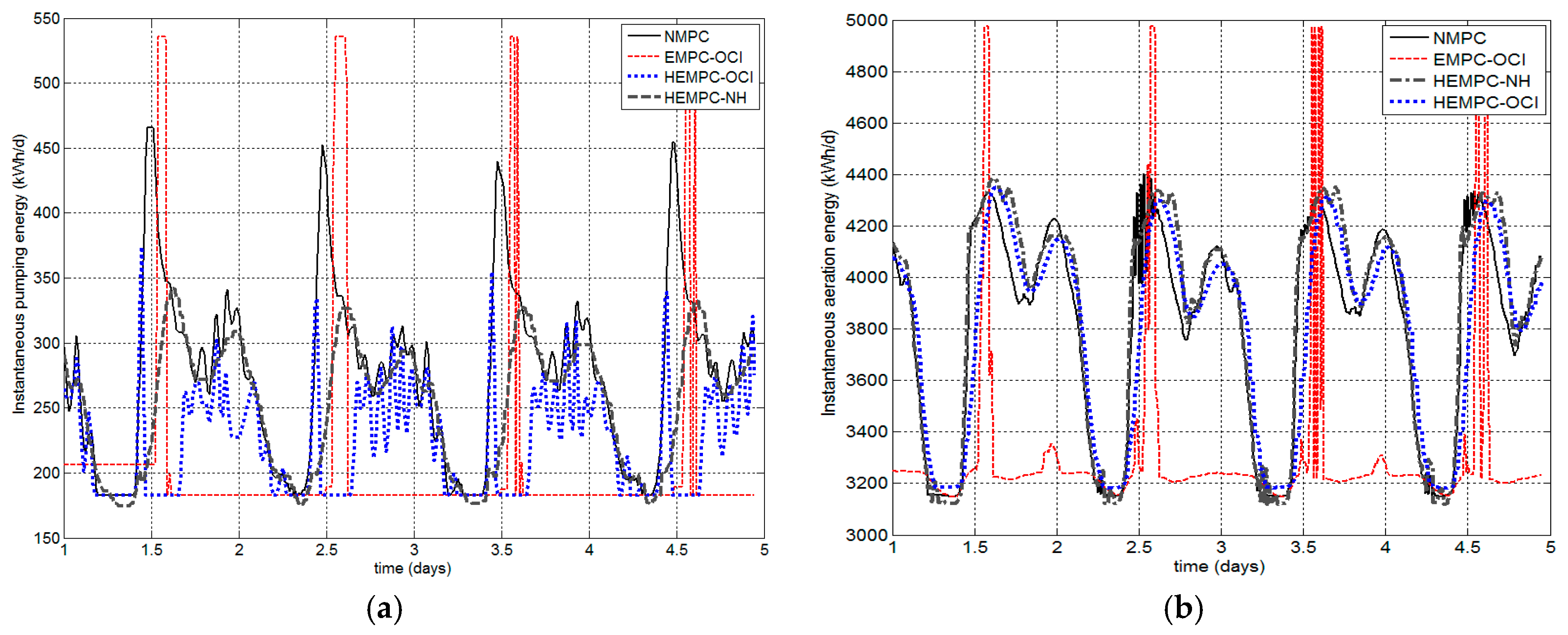
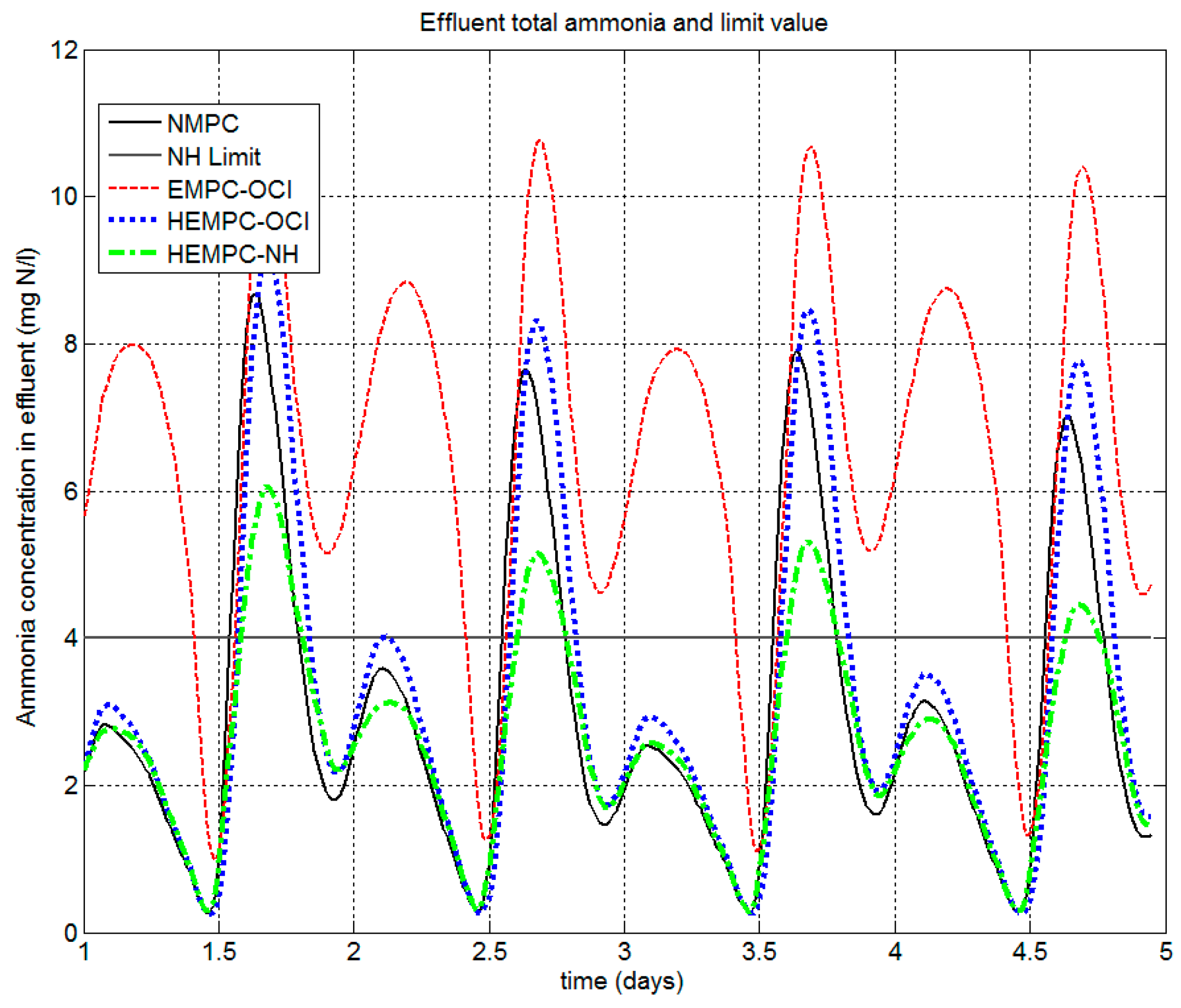
The instantaneous values of the aeration energy and the pumping energy along the operation period are presented in Figure 8 for the most representative EMPC and HEMPC designs, and the corresponding ammonium concentration in the effluent is presented in Figure 9. In general, higher weights of the OCI (EMPC-OCI, HEMPC-OCI) improve economics, but increase the violations of the limit of ammonium in the effluent, since SO5 levels are reduced to minimize aeration costs. On the other hand, the minimization of the violation fines of the required effluent quality (HEMPC-NH, EMPC-NH) increases the OCI. However, that increase in the OCI is associated with the aeration energy to reduce the levels of ammonium, since the internal recycle flow decreases when ammonium concentration is minimized, as observed in the figures.
The performance indices calculated for the overall operation period with the proposed controllers are presented in Table 2 and Table 3, respectively. The influent profile described in the BSM1 for dry weather (Figure 2) is used to evaluate the plant performance over an operation period of four days, the first day with constant influent. The influent quality index defined in [22] to measure the pollution load of the influent is IQ = 55,945.14 kg-pollutants/day. The indices computed for the default BSM1 strategy are included also for comparison. Table 2 contains the indices associated with the variables considered in the economic-oriented model predictive controller optimization, to show that performance indices vary according to the relative importance given to each objective in the optimization. In general, all the EMPC designs improve the pumping energy with respect to the NMPC and PI default strategies based on set-point tracking. A reduction in the energy costs (AE + PE) of 13% with respect to the NMPC is achieved, with the pure EMPC focused on the optimization of the energy costs (EMPC-OCI). Ammonium concentration in the effluent reduces by 21% when the EMPC is focused on the minimization of the off-specification ammonium concentration in the effluent. Comparing with the default BSM1 PI strategy, a reduction of the energy costs of 13% is achieved also with the EMPC-OCI, produced especially by a decrease in the pumping energy of up to 23%.
Table 3 is presented to show that additional process variables are affected by the economic optimization, and it is possible to include them in the optimization. The OCI index reported in Table 3 corresponds to the BSM1 performance index, which includes aeration energy, pumping energy, mixing energy and sludge production costs.
In order to compare with the previous work of Zeng and Liu [16], Table 4 presents the changes in the performance indices, with respect to the operation with the BSM1 default PI strategy in the same simulation scenario. The comparison is made with selected designs with analogous tuning parameters. The EMPC proposed in this work enhances the economic performance mainly by reducing the pumping energy in all the cases, and the aeration energy in the EMPC-OCI design, which are the operation costs considered in the economic function. In the Zeng and Liu [16] formulation, the BSM1 overall cost index (OCI) is optimized; it includes aeration and pumping energy, but also the mixing energy and the costs of sludge disposal. Then, an operation with small energy consumption with respect to the default PI strategy is achieved in general, but pumping aeration costs are larger than those obtained with the methodology proposed here. On the other hand, since the effluent quality index is included as an optimization objective in the Zeng and Liu [16] formulation, the improvement in this index is notorious, while the advantages of the EMPC formulation proposed in this paper are associated with the economic performance. In the current work, it has been preferred to not work directly with the overall effluent quality index as part of the cost function, because it involves several concentrations not available for measurement. Instead, here, it has been preferred to keep the two main variables of interest (oxygen and nitrate) around desired values, while attempting to keep effluent ammonia under the established limits.
Regarding this reduction in energy consumption, as the work conducted here is based on the BSM1 benchmark scenario, no specific WWTP was used. However, the BSM1 protocols define influent characteristics featuring a load of around 100,000 person equivalents (PE) (80,000 from households, and 20,000 from industrial origin). This helps to provide an idea of the repercussion of the mentioned energy savings. Of course, in order to get concrete monetary figures of actual order, there will be the need to link the cost indexes to actual energy costs. This may be highly dependent on the WWTP location. However, just to point to some figures, according to HUBER Technology (http://www.picatech.ch/solutions/energy-efficiency), power consumption of state-of-the-art wastewater treatment plants should be around 45 kWh/(PE.a) for plants serving >100,000 PE, where pumping and aeration are recognized primary power consumers.
4. Conclusions
In this paper, a successful implementation of a single-layer economic oriented model predictive control approach for the optimization of the operation of wastewater treatment plants (WWTPs) in a simulation environment is presented. Even though this study used empirical models based on data gathering and the adequate software and communication systems, the technique could be implemented in real plants.
An OCI reduction of 13% with respect to the standard NMPC focused on set-point tracking is achieved, with the pure EMPC focused on the optimization of the energy costs (EMPC-OCI), and ammonium concentration in the effluent reduces by 21% when using the EMPC focused on the minimization of the off-specification ammonium concentration in the effluent. Those improvements are achieved by performing a dynamic optimization of the operation, taking advantage of the variations in the load to find more favourable operating conditions on a given operating window.
The results demonstrate that the implementation of novel advanced control techniques as single-layer EMPCs can produce significant energy savings and improvements in WWTP performance. The single-layer strategy has the advantage of being simpler than other strategies, e.g., [9], which obtain further reductions in costs but with a more complex hierarchical framework for nitrate and oxygen control. On the other hand, in the pioneering implementation of EMPCs to the BSM1 model presented in [16] the full model is used for predictions, therefore, a novel feature presented in this work is the implementation of techniques to face modeling errors. It is also encouraging the potential use of a reduced model with partial information with prediction purposes. Alternative formulations oriented towards the increase of model quality should be investigated, as they will have a direct repercussion on the final quality of the obtained control.
Future work is oriented to exploit these characteristics in different scenarios, and introduce additional optimization objectives in the economic-oriented controller formulation. It is encouraging to promote continuing research in the application of these advanced control strategies to improve WWTP operation.
Acknowledgments
The authors wish to thank the support of the Spanish Government through the Ministerio de Economía y Competitividad (MINECO) projects DPI2015-67341-C2-1-R, DPI2016-77271-R also with FEDER funding. The Samuel Solórzano Foundation through project FS/21-2015 and the IWA Task Group from the Department of Industrial Electrical Engineering and Automation (IEA), Lund University, Sweden (Ulf Jeppsson, Christian Rosen) for the BSM1 models.
Author Contributions
Pastora Vega and Ramón Vilanova conceived and designed the experiments; Silvana Revollar performed the experiments and Silvana Revollar and Mario Francisco analyzed the results; all the authors have contributed to write the paper.
Conflicts of Interest
The authors declare no conflict of interest.
Appendix A
The BSM1 platform uses the Activated Sludge Process No1 (ASM1) to represent the behavior of the biological reactors. It uses 13 state variables on each reactor, and considers eight biological processes such as heterotrophic and autotrophic biomass growth in anoxic and aerobic conditions and biomass decay, ammonification of soluble organic nitrogen, hydrolysis of entrapped organics, and hydrolysis of entrapped organic nitrogen. In the reduced model used in this work, only the faster biological processes are taken into account: the growth of heterotrophic biomass in aerobic conditions (), the growth of heterotrophic biomass in anoxic conditions (), and the growth of autotrophic biomass in aerobic conditions (). The plant is reduced to one anoxic reactor and one aerobic reactor, with a volume equivalent to the anoxic and aerobic zones of the BSM1, respectively. The concentration of autotrophic and heterotrophic biomass in the reactors is assumed to be constant (XB,H = 2500 mg/L, XB,A = 150 mg/L). These constant values are taken from [17] and correspond to the steady state values at the biological reactors. The influent variables considered in the reduced model are: the influent flow (Qin), the organic matter concentration (SS,in), and the ammonium concentration (SNH,in). The index i is used to distinguish the units, with reactor 1 the anoxic zone (i = 1), and reactor 2 the aerobic zone (i = 2). The states associated to the faster biological processes are: the concentration of ammonium compounds (SNHi), the concentration of nitrates (SNOi), the organic matter concentration (SSi) and the oxygen concentration (SOi). The inputs are the oxygen transfer coefficient (KLa) and the internal recycle flow (Qa).
Regarding the comparison with real plants measurements, although the BSM1 model variables and reduced model variables differ from the variables typically measured in real wastewater treatment plants, it is possible to form a relationship between their values. Some equations to compute COD (chemical oxygen demand), BOD (Biological oxygen demand) and other typical wastewater measurements from the BSM1 variables are presented in Alex et al. [22].
A list of the process parameters and variables considered in the reduced model used here are presented in Table A1.

Table A1.
Reduced BSM1 model variables and parameters for a temperature close to T = 15 °C.
| Description | Name | Values |
|---|---|---|
| Process variables | ||
| Anoxic reactor volume (m3) | V1 | 2000 |
| Aerobic reactors volume (m3) | V2 | 3999 |
| Active heterotrophic biomass concentration (gr COD/m3) | XB.H | 2500 |
| Active autotrophic biomass concentration (gr COD/m3) | XB,A | 150 |
| Dissolved oxygen concentration (gr COD/m3) | SO | 0.1–5 |
| Nitrate and nitrite concentration (gr N/m3) | SNO | 0.1–5 |
| NH4+ + NH3 concentration (gr N/m3) | SNH | 0–14 |
| Readily biodegradable substrate concentration (gr COD/m3) | SS | 0–40 |
| Influent flow rate (m3/h) | Qin | 45–2500 |
| Effluent flow rate (m3/h) | Qe | 45–2500 |
| Readily biodegradable substrate concentration in the influent (gr COD/m3) | SS,in | 45–140 |
| Ammonium compounds concentration in the influent (gr N/m3) | SNH,in | 8–55 |
| Internal recycle flow (m3/h) | Qa | 180–2000 |
| Oxygen transfer coefficient (1/h) | KLa | 0–10 |
| Biological processes parameters | ||
| Oxygen saturation concentration (gr/m3) | SO,sat | 8 |
| Heterotrophic max. specific growth rate (1/day) | 4 | |
| Half saturation coefficient for heterotrophs (gr COD/m3) | Ks | 10 |
| Oxygen saturation coefficient for heterotrophs (gr COD/m3) | KO,H | 0.2 |
| Ammonia saturation coefficient for heterotrophs (grN/m3) | KNH | 1 |
| Oxygen saturation coefficient for autotrophs (gr COD/m3) | KO,A | 0.4 |
| Heterotrophic yield (gr cell COD formed/gr COD oxydized) | YH | 0.67 |
| Autotrophic yield (gr cell COD formed/gr N oxydized) | YA | 0.24 |
| Nitrogen fraction in biomass (gr N/gr COD) | iXB | 0.08 |
The equations of the mathematical model are the following:
Biological processes:
Differential equations given by the mass balances:
Appendix B
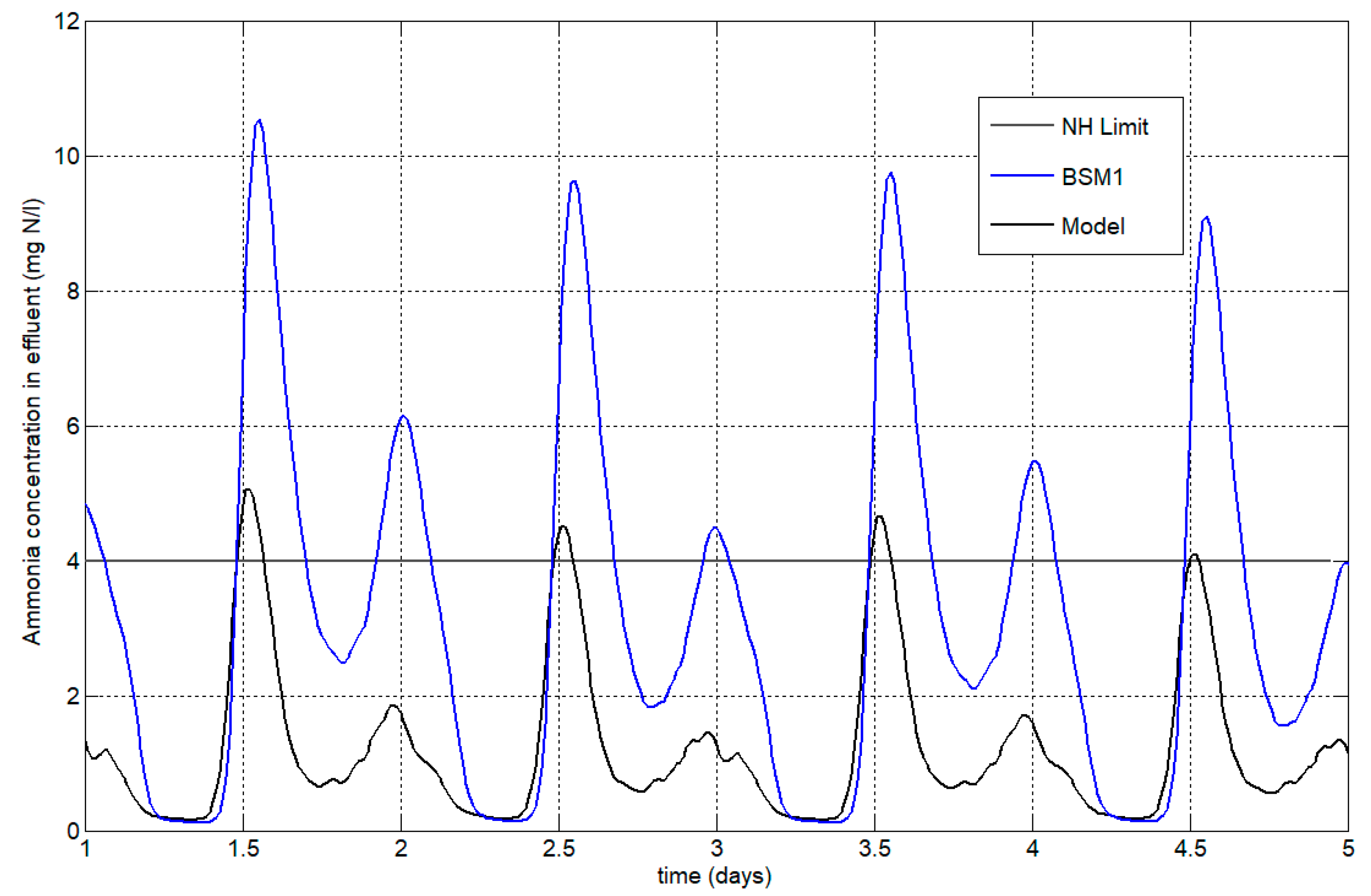
The comparison between the reduced model responses and the BSM1 model responses of the most relevant variables for the controller optimization, namely, nitrates concentration at the end of the anoxic zone (SNO2 in BSM1, SNO1 in reduced model), oxygen concentration at the end of the aerobic zone (SO5 in BSM1, SO2 in reduced model), and ammonium concentration at the end of the aerobic zone (SNH5 in BSM1, SNH2 in reduced model), is presented in Figure A1, Figure A2 and Figure A3.
The model behavior is similar to BSM1 response in the evaluated conditions; however, a significant difference in the magnitude of the variables is observed. However, in the evaluation of model for predictions in the controller executions, the difference is lowered, since an initial state given by the measured BSM1 states is provided.
It is important to highlight that the objective of the work is not the development of an accurate reduced BSM1 model. The objective is to evaluate the performance of the single-layer EMPC for optimizing economics in the presence of modeling errors.
The reduced model represents the variables with the faster dynamics, which are directly affected by control actions, and are optimized each sampling time (5 min in this implementation). Even though the hydrolysis of particulate matters is relevant in the biological processes that take place in the activated sludge process, its dynamics can be neglected in these applications. A sensitivity analysis of an accurately reduced model considering the different dynamics of the biological processes is presented in [29].
Figure A1.
Comparison of the reduced model and BSM1 evolution of the nitrates concentration in the second anoxic reactor obtained in the open loop operation using the manipulated variables values that produce the nominal set points.
Figure A1.
Comparison of the reduced model and BSM1 evolution of the nitrates concentration in the second anoxic reactor obtained in the open loop operation using the manipulated variables values that produce the nominal set points.
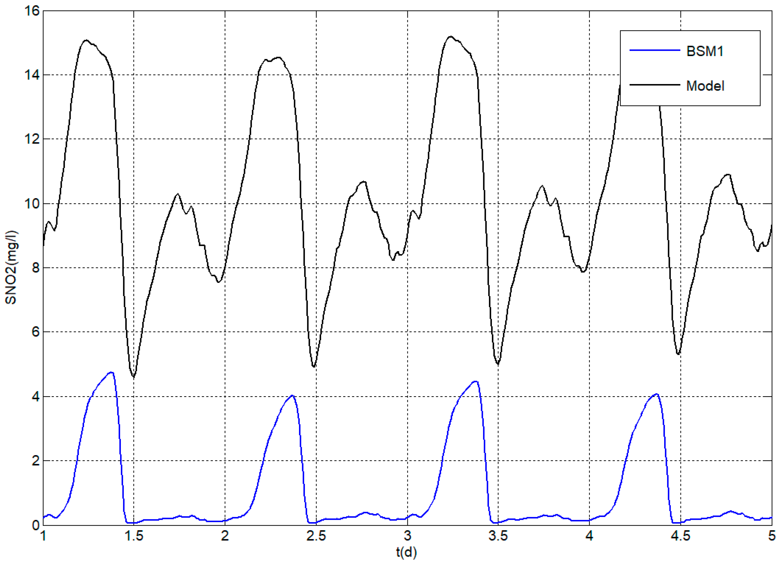
Figure A2.
Comparison of the reduced model and BSM1 evolution of the oxygen concentration in the fifth reactor (aerobic) obtained in the open loop operation, using the manipulated variables values that produce the nominal set points.
Figure A2.
Comparison of the reduced model and BSM1 evolution of the oxygen concentration in the fifth reactor (aerobic) obtained in the open loop operation, using the manipulated variables values that produce the nominal set points.

Figure A3.
Comparison of the reduced model and BSM1 evolution of the ammonia concentration in the effluent obtained in the open loop operation using the manipulated variables values that produce the nominal set points.
Figure A3.
Comparison of the reduced model and BSM1 evolution of the ammonia concentration in the effluent obtained in the open loop operation using the manipulated variables values that produce the nominal set points.
References
- Olsson, G.; Nielsen, M.; Yuan, Z.; Lynggaard-Jensen, A.; Steyer, J.-P. Instrumentation, Control and Automation in Wastewater Systems; IWA Publishing: London, UK, 2005. [Google Scholar]
- Olsson, G. ICA and me a subjective review. Water Res. 2012, 46, 1585–1624. [Google Scholar] [CrossRef] [PubMed]
- Santin, I.; Pedret, C.; Vilanova, R. Control and Decision Strategies in Wastewater Treatment Plants for Operation Improvement; Springer: Cham, Switzerland, 2016. [Google Scholar]
- Gernaey, K.; Rosen, C.; Jeppsson, U. BSM2: A Model for Dynamic Influent Data Generation; Technical Report; Lund University: Lund, Sweden, 2005. [Google Scholar]
- Amand, L.; Olsson, G.; Carlsson, B. Aeration Control—A review. Water Sci. Technol. 2013, 67, 2374–2397. [Google Scholar] [CrossRef] [PubMed]
- O’Brien, M.; Mack, J.; Lennox, B.; Lovett, D.; Wall, A. Model predictive control of an activated sludge process: A case study. Control Eng. Pract. 2011, 19, 54–61. [Google Scholar] [CrossRef]
- Santín, I.; Pedret, C.; Vilanova, R. Fuzzy control and model predictive control configurations for effluent violations removal in wastewater treatment plants. Ind. Eng. Chem. Res. 2015, 54, 2763–2775. [Google Scholar] [CrossRef]
- Vega, P.; Revollar, S.; Francisco, M.; Martin, J.M. Integration of set point optimization techniques into nonlinear MPC for improving the operation of WWTPs. Comput. Chem. Eng. 2014, 68, 78–95. [Google Scholar] [CrossRef]
- Santín, I.; Pedret, C.; Vilanova, R. Applying variable dissolved oxygen set point in a two level hierarchical control structure to a wastewater treatment process. J. Process Control 2015, 28, 40–55. [Google Scholar] [CrossRef]
- Santín, I.; Pedret, C.; Vilanova, R.; Meneses, M. Removing violations of the effluent pollution in a wastewater treatment process. Chem. Eng. J. 2015, 279, 207–219. [Google Scholar] [CrossRef]
- Piotrowski, R.; Brdys, M.A.; Konarczak, K.; Duzinkiewicz, K.; Chotkowski, W. Hierarchical dissolved oxygen control for activated sludge processes. Control Eng. Pract. 2008, 16, 114–131. [Google Scholar] [CrossRef]
- Brdys, M.A.; Grochowski, M.; Gminski, T.; Konarczak, K.; Drewa, M. Hierarchical predictive control of integrated wastewater treatment systems. Control Eng. Pract. 2008, 16, 751–767. [Google Scholar] [CrossRef]
- Darby, M.L.; Nikolau, M.; Jones, J.; Nicholson, D. RTO: An overview and assessment of current practice. J. Process Control. 2011, 21, 874–884. [Google Scholar] [CrossRef]
- Tatjewski, P. Advanced control and on-line process optimization in multilayer structures. Ann. Rev. Control 2008, 32, 71–85. [Google Scholar] [CrossRef]
- Revollar, S.; Vega, P.; Vilanova, R.; Francisco, M.; Santín, I. Optimization of Economic and Environmental Objectives in a Non Linear Model Predictive Control Applied to a Wastewater Treatment Plant. In Proceedings of the 20th ICSTCC, Sinaia, Romania, 13–15 October 2016. [Google Scholar]
- Zeng, J.; Liu, J. Economic model predictive control of wastewater treatment processes. Ind. Eng. Chem. Res. 2015, 54, 5710–5721. [Google Scholar] [CrossRef]
- Ellis, M.; Duranda, H.; Christofides, P. A tutorial review of economic model predictive control methods. J. Process Control 2014, 24, 1156–1178. [Google Scholar] [CrossRef]
- Würth, L.; Hannemann, R.; Marquardt, W. A two-layer architecture for economically optimal process control and operation. J. Process Control 2011, 21, 309–436. [Google Scholar] [CrossRef]
- Engell, S. Feedback control for optimal process operation. J. Process Control 2007, 17, 203–219. [Google Scholar] [CrossRef]
- Forbes, J.F.; Marlin, T.E. Model accuracy for economic optimizing controllers: The bias update case. Ind. Eng. Chem. Res. 1994, 33, 1919–1929. [Google Scholar] [CrossRef]
- Samuelsson, P.; Halvarsson, B.; Carlsson, B. Cost-efficient operation of a denitrifying activated sludge process. Water Res. 2007, 41, 2325–2332. [Google Scholar] [CrossRef] [PubMed]
- Alex, J.; Benedetti, L.; Copp, J.; Gernaey, K.; Jeppsson, U.; Nopens, I.; Pons, M.; Rieger, L.; Rosen, C.; Steyer, J.; et al. Benchmark Simulation Model No. 1 (BSM1), IWA Taskgroup on Benchmarking of Control Strategies for WWTPs; Cod.: LUTEDX-TEIE 7229. 1-62; Department of Industrial Electrical Engineering and Automation, Lund University: Lund, Sweden, 2008. [Google Scholar]
- Maciejowski, J.M. Predictive Control with Constraints; Prentice Hall: Upper Saddle River, NJ, USA, 2002. [Google Scholar]
- Qin, S.; Badgwell, T. A survey of industrial model predictive control technology. Control Eng. Pract. 2003, 11, 733–764. [Google Scholar] [CrossRef]
- Ochoa, S.G.; Wozny, G.; Repke, J.U. Plantwide Optimizing Control of a continuous bioethanol production process. J. Process Control 2010, 20, 983–998. [Google Scholar] [CrossRef]
- Idris, E.; Engell, S. Economics-based NMPC strategies for the operation and control of a continuous catalytic distillation process. J. Process Control 2012, 22, 1832–1843. [Google Scholar] [CrossRef]
- Takács, I.; Patry, G.G.; Nolasco, D. A dynamic model of the clarification thickening process. Water Res. 1991, 25, 1263–1271. [Google Scholar] [CrossRef]
- Vilanova, R.; Santín, I.; Pedret, C. Control y Operación de Estaciones Depuradoras de Aguas Residuales: Modelado y Simulación. Revista Iberoamericana de Automática e Informática Industrial RIAI 2017, 14, 217–233. [Google Scholar] [CrossRef]
- Cadet, C.; Bèteau, S.; Hernández, C. Multicriteria control strategy for cost/quality compromise in Wastewater Treatment Plants. Control Eng. Pract. 2004, 12, 335–347. [Google Scholar] [CrossRef]
Figure 1.
Benchmark simulation model (BSM1) layout indicating the default control strategy. PI: Proportional Integral Controller; DO: Dissolved oxygen.
Figure 1.
Benchmark simulation model (BSM1) layout indicating the default control strategy. PI: Proportional Integral Controller; DO: Dissolved oxygen.

Figure 2.
Influent profile for a four-day operating horizon.

Figure 3.
Proposed control strategy in the BSM1 layout indicating the measured variables: nitrates concentration in the second anoxic reactor, oxygen concentration in the last aerobic reactor, and the manipulated variables Qa and KLa.
Figure 3.
Proposed control strategy in the BSM1 layout indicating the measured variables: nitrates concentration in the second anoxic reactor, oxygen concentration in the last aerobic reactor, and the manipulated variables Qa and KLa.

Figure 4.
BSM1-controlled variables’ responses under NMPC and economic-oriented tracking controllers (Hybrid-EMPC or HEMPC). (a) Nitrates and nitrites concentration in the second rector (SNO2) response (b) dissolved oxygen in the last aerobic reactor (SO5) response. NMPC: non-linear model predictive controller; OCI: overall cost index.
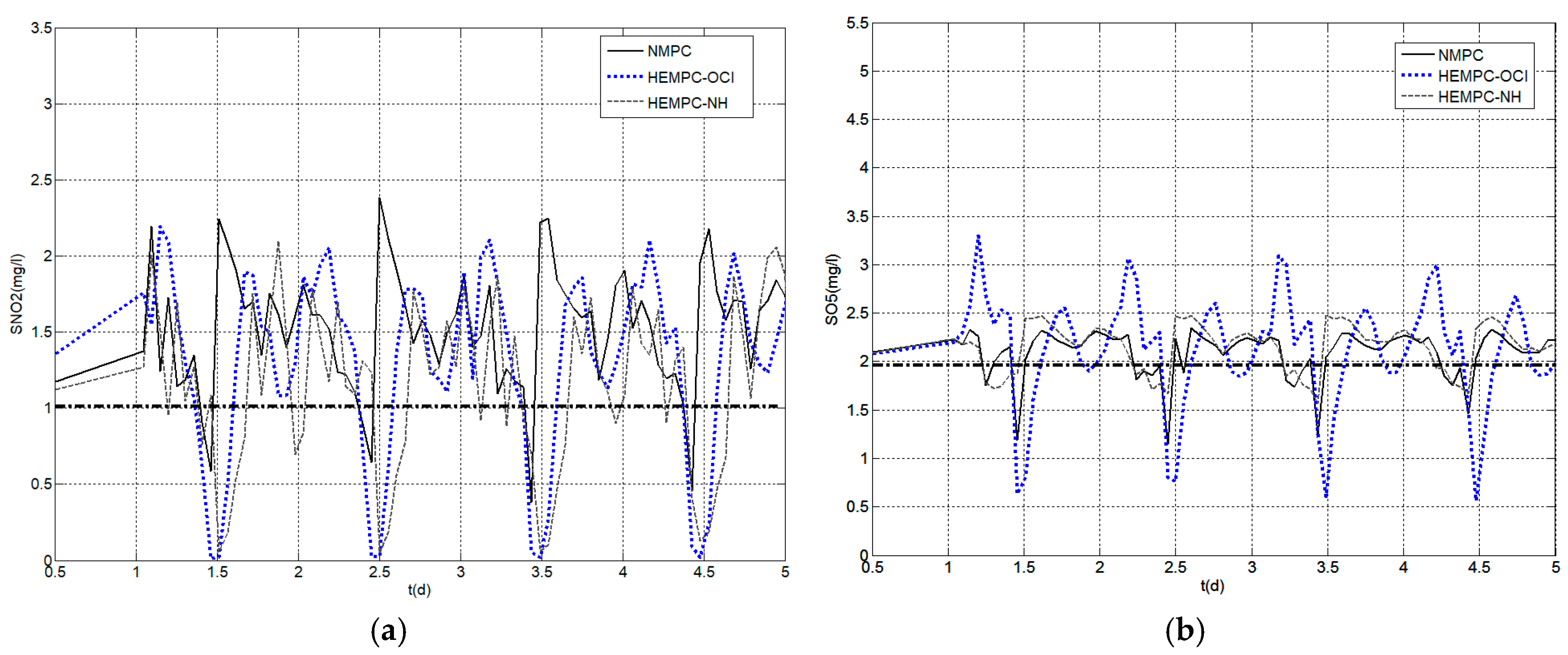
Figure 5.
Control signals applied to the BSM1 plant operating under NMPC and HEMPC controllers. (a) Internal recycle flow (Qa) (b) oxygen transfer coefficient (KLa).
Figure 5.
Control signals applied to the BSM1 plant operating under NMPC and HEMPC controllers. (a) Internal recycle flow (Qa) (b) oxygen transfer coefficient (KLa).
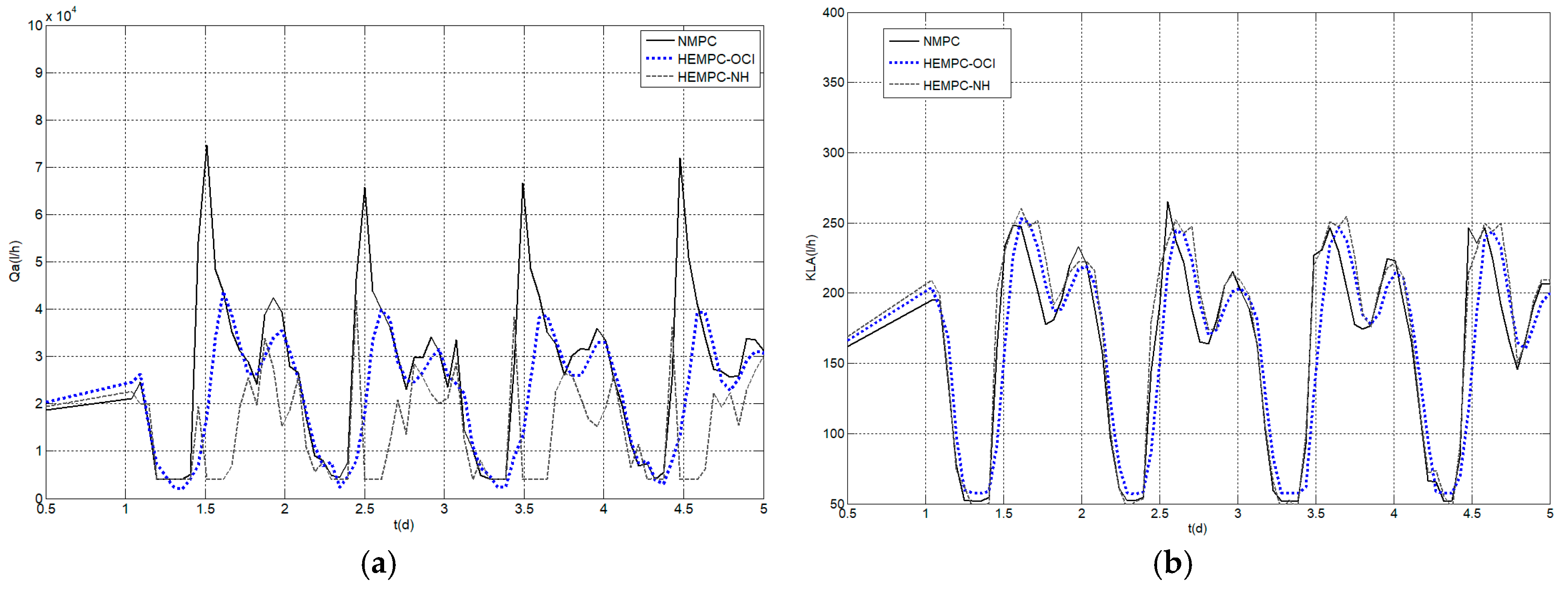
Figure 6.
BSM1-controlled variables’ responses under NMPC and EMPC controllers. (a) Nitrates and nitrites concentration in the second rector (SNO2) response (b) dissolved oxygen in the last aerobic reactor (SO5) response. EMPC: economic-oriented model predictive controller.
Figure 6.
BSM1-controlled variables’ responses under NMPC and EMPC controllers. (a) Nitrates and nitrites concentration in the second rector (SNO2) response (b) dissolved oxygen in the last aerobic reactor (SO5) response. EMPC: economic-oriented model predictive controller.
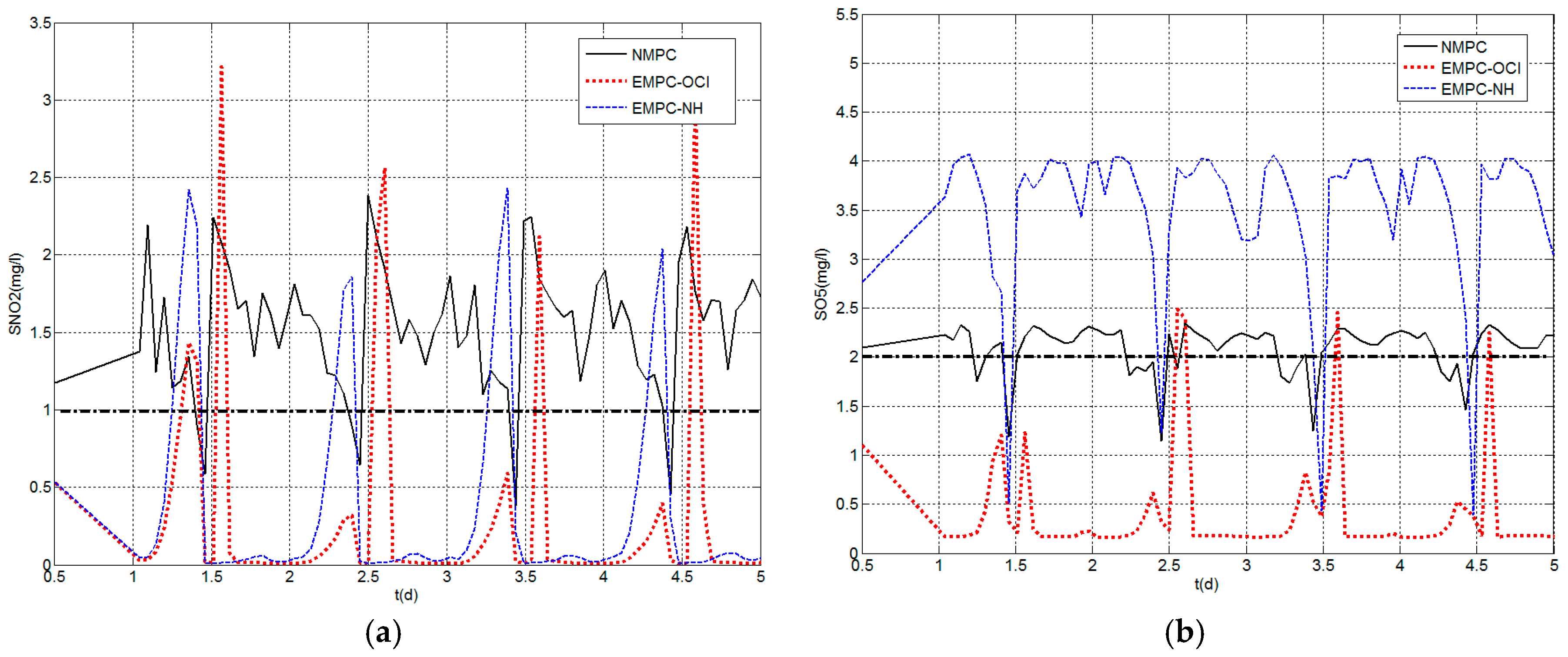
Figure 7.
Control signals applied to the BSM1 plant operating under NMPC and EMPC controllers. (a) Internal recycle flow (Qa) (b) oxygen transfer coefficient (KLa).
Figure 7.
Control signals applied to the BSM1 plant operating under NMPC and EMPC controllers. (a) Internal recycle flow (Qa) (b) oxygen transfer coefficient (KLa).

Figure 8.
Instantaneous pumping (a) and aeration energy (b) for the BSM1 plant operating under selected controllers.
Figure 8.
Instantaneous pumping (a) and aeration energy (b) for the BSM1 plant operating under selected controllers.

Figure 9.
Ammonium concentration in the effluent for selected controller designs.

Table 1.
Effluent quality limits.
| Variable | Bound |
|---|---|
| Total Nitrogen (TN) | <18 grN/m3 |
| Chemical Oxygen Demand (COD,e) | <100 grCOD/m3 |
| Ammonium concentration (SNH,e) | <4 grN/m3 |
| Nitrate concentration (SNO,e) | <10 grN/m3 |
Table 2.
Performance indices associated with variables of the plant optimized in the economic oriented model predictive controllers cost function (computed for a four-day operation period under dry weather disturbances). NMPC: non-linear model predictive controller; HEMPC: economic-oriented tracking controller; OCI: overall cost index penalization; NH: off-specification ammonium load in the effluent penalization; EMPC: economic-oriented model predictive controller.
| Controller | Average SNH in the Effluent (mg/L) | EQ (kg/Day) | AE (kWh/Day) | PE (kWh/Day) | PE + AE (EUR/Day) | SNH Violations (Days) |
|---|---|---|---|---|---|---|
| Default PI | 2.79 | 6587.7 | 3785 | 268.0 | 4053.0 | 0.84 |
| NMPC | 3.00 | 6573.8 | 3802 | 276.6 | 4078.6 | 0.96 |
| HEMPC-OCI | 3.21 | 6783.9 | 3796 | 252.8 | 4048.8 | 1.00 |
| HEMPC-OCI + NH | 2.74 | 6584.7 | 3830 | 246.8 | 4076.8 | 0.88 |
| HEMPC-NH | 2.55 | 6698.0 | 3855 | 224.8 | 4079.8 | 0.73 |
| EMPC-OCI | 6.05 | 8289.0 | 3310 | 206.0 | 3516.0 | 3.34 |
| EMPC-OCI + NH | 3.47 | 7617.0 | 3841 | 167.2 | 4008.2 | 1.15 |
| EMPC-NH | 2.37 | 7315.3 | 4277 | 166.0 | 4443.0 | 0.74 |
Table 3.
Performance indices of the mean operating variables of the plant that are different from the variables included in the optimization problem (computed for a four-day operation period under dry weather disturbances).
Table 3.
Performance indices of the mean operating variables of the plant that are different from the variables included in the optimization problem (computed for a four-day operation period under dry weather disturbances).
| Controller | Average SNH in the Effluent (mg/L) | TN (mg/L) | Sludge Produced (kg/Day) | OCI (EUR/Day) | SNH Violations (Days) | TN Violations (Days) |
|---|---|---|---|---|---|---|
| Default PI | 2.79 | 17.2 | 2747.0 | 18,031 | 0.84 | 0.98 |
| NMPC | 3.00 | 16.7 | 2747.3 | 18,055 | 0.96 | 0.73 |
| HEMPC-OCI | 3.21 | 17.4 | 2746.6 | 18,021 | 1.00 | 0.94 |
| HEMPC-OCI + NH | 2.74 | 17.3 | 2747.0 | 18,052 | 0.88 | 0.87 |
| HEMPC-NH | 2.55 | 18.2 | 2748.0 | 18,064 | 0.73 | 1.47 |
| EMPC-OCI | 6.05 | 19.5 | 2741.9 | 17,466 | 3.34 | 3.60 |
| EMPC-OCI + NH | 3.47 | 21.2 | 2748.0 | 17,988 | 1.15 | 3.80 |
| EMPC-NH | 2.37 | 21.8 | 2750.0 | 18,434 | 0.74 | 3.95 |
Table 4.
Performance indices variation respect to the BSM1 PI default strategy.
| Controller | % AE Variation | % PE Variation | % OCI Variation |
|---|---|---|---|
| EMPC-OCI | −12.55 | −23.13 | −3.13 |
| EMPC-OCI + NH | 1.47 | −37.61 | −0.24 |
| EMPC-NH | 13.00 | −38.06 | 2.24 |
| Zeng and Liu EMPC-NH | 3.73 | 3.30 | −9.78 |
| Zeng and LiuEMPC-OCI + NH | −3.40 | 6.75 | −11.18 |
© 2017 by the authors. Licensee MDPI, Basel, Switzerland. This article is an open access article distributed under the terms and conditions of the Creative Commons Attribution (CC BY) license (http://creativecommons.org/licenses/by/4.0/).
Share and Cite
MDPI and ACS Style
Revollar, S.; Vega, P.; Vilanova, R.; Francisco, M. Optimal Control of Wastewater Treatment Plants Using Economic-Oriented Model Predictive Dynamic Strategies. Appl. Sci. 2017, 7, 813. https://doi.org/10.3390/app7080813
AMA Style
Revollar S, Vega P, Vilanova R, Francisco M. Optimal Control of Wastewater Treatment Plants Using Economic-Oriented Model Predictive Dynamic Strategies. Applied Sciences. 2017; 7(8):813. https://doi.org/10.3390/app7080813
Chicago/Turabian StyleRevollar, Silvana, Pastora Vega, Ramón Vilanova, and Mario Francisco. 2017. "Optimal Control of Wastewater Treatment Plants Using Economic-Oriented Model Predictive Dynamic Strategies" Applied Sciences 7, no. 8: 813. https://doi.org/10.3390/app7080813
Note that from the first issue of 2016, this journal uses article numbers instead of page numbers. See further details here.