Pollutant Recognition Based on Supervised Machine Learning for Indoor Air Quality Monitoring Systems

Abstract

Indoor air may be polluted by various types of pollutants which may come from cleaning products, construction activities, perfumes, cigarette smoke, water-damaged building materials and outdoor pollutants. Although these gases are usually safe for humans, they could be hazardous if their amount exceeded certain limits of exposure for human health. A sophisticated indoor air quality (IAQ) monitoring system which could classify the specific type of pollutants is very helpful. This study proposes an enhanced indoor air quality monitoring system (IAQMS) which could recognize the pollutants by utilizing supervised machine learning algorithms: multilayer perceptron (MLP), K-nearest neighbour (KNN) and linear discrimination analysis (LDA). Five sources of indoor air pollutants have been tested: ambient air, combustion activity, presence of chemicals, presence of fragrances and presence of food and beverages. The results showed that the three algorithms successfully classify the five sources of indoor air pollution (IAP) with a classification rate of up to 100 percent. An MLP classifier with a model structure of 9-3-5 has been chosen to be embedded into the IAQMS. The system has also been tested with all sources of IAP presented together. The result shows that the system is able to classify when single and two mixed sources are presented together. However, when more than two sources of IAP are presented at the same period, the system will classify the sources as ‘unknown’, because the system cannot recognize the input of the new pattern.

1. Introduction

The issue of outdoor air pollution (OAP), such as haze, is well known to the public due to the attention given to it by the media. In contrast, the issue of indoor air pollution (IAP) is less known to the public, although IAP poses similar threats towards human health. In fact, more attention should be given to the issue of IAP, because people normally spend 90% of their time in indoor environments [1]. IAP, which undermines indoor air quality (IAQ), is found to contain indoor air pollutants such as harmful gases and contaminants at a concentration level up to five times higher than the concentration of these pollutants in normal air. In severe cases, the concentration level of the pollutants could rise up to 100 times more than a normal concentration level, which is hazardous for human health [1].

IAP can be defined as the disturbance of any gases, materials or human activities on the state of ambient air in indoor environment [2]. In other words, IAP does not need the presence of disease or infirmity. As long as the concentration in the normal ambient air is disturbed either by gases, other materials or combustion activity, it is already considered as pollution. The most common sources of IAP are contributed by combustion activities such as cigarette smoking, wood or paper burning, gas stoves, gas-fired dryers and engines emission [3,4]. Other materials, such as chemical products, building materials and office materials, are also major sources of IAP. Chemical products such as air fresheners and cleaning products contribute to IAP by emitting volatile organic compounds (VOCs), while building and office materials such as printers and carpets also release air contaminants such as dust into the indoor air atmosphere [5,6,7,8,9]. IAP may also emerge as a result of variations of gas concentration in the indoor air, as well as from variations in thermal conditions such as temperature and humidity [10,11]. Thermal or physical conditions such as temperature, relative humidity (RH) and air movement are important IAP parameters as they could affect people’s perception towards IAP. These physical parameters can act directly on building occupants, interact with indoor air pollution factors or affect human responses to the indoor environment [12,13,14,15,16]. These sources of IAP might not look harmful, but to a certain extent (based on the concentration level) they may be hazardous to human health.

The health effects from IAP may be experienced soon after exposure, or possibly, years later, depending on the individuals and type of pollutants they have been exposed to [17]. The common health conditions that may show up immediately include irritation of the eyes, nose, and throat, headaches, dizziness, fatigue, asthma and humidifier fever. The health effects of years of exposure to IAP are more dangerous and can be fatal; these include some respiratory-related diseases, heart disease, and cancer [18,19]. The health effects relating to poor indoor air quality have been divided into four categories: environmental tobacco smoke (ETS), sick building syndrome (SBS), building related illness (BRI), and thermal comfort problems (TCP) [10,13,20]. Hence, meticulous attention should be given to make sure the indoor air is safe and comfortable.

Indoor air may be polluted by various types of pollutants which may come from cleaning products, construction activities, perfumes, cigarette smoke, water-damaged building materials and outdoor pollutants [21]. Although these gases are usually safe for humans, they could be hazardous to human beings, especially people with respiratory-related problem and children, if their amount exceeded certain limits of exposure for human health. In terms of the current technology, certain sensing devices have allowed researchers to get continuous, quick and reliable information about ambient air [21] which enable advanced data processing to be applied to the data of ambient air. Forecasting techniques allow the system to predict level of IAQ while pattern recognition techniques allow the system to recognize certain types of smell. However, these advanced data processing techniques were mainly used to investigate the odour in outdoor environments [22,23,24,25]. In indoor environments, odour recognition was usually used to detect odour from a single category; for example, the use of odour recognition to recognize types of mushrooms [26], types of oil flowers (lavender, hyssop, geranium and rosemary) [27] or types of pure chemical only (ethanol, hexanal, linalool, and ammonia) [28]. On the other hand, some other techniques, such as computational fluid dynamics (CFD), are used to predict IAP in indoor environments [29,30]. CFD is used to evaluate the IAQ for buildings near to the road traffic environment.

This study proposed an enhancement of the IAQMS, where the system is integrated with sources of pollution recognition. The proposed IAQMS has been developed and designed using an array of sensors which can also effectively function as an electronic nose, meaning that it could measure multiple pollutants that influenced indoor air levels. The pattern recognition algorithm allows the system to recognize the sources of IAP from five conditions: ambient air, combustion activity, presence of fragrance, presence of chemical and presence of food and beverages. As for the sources influencing IAP recognition ability, this study utilized a machine learning algorithm that is widely used in data mining. In order to find the best classifier among the family of machine learning algorithms, three algorithms which have been used in many applications—especially involving odour or smell classification—have been chosen. The three algorithms chosen are multilayer perceptron (MLP), K-nearest neighbour (KNN) and linear discrimination analysis (LDA). Then, the classifier that provided the best classification results is chosen to be embedded into the system.

2. Overview of Developed IAQMS System

Basically, the developed system consists of the sensor module cloud (SMC), base station and service-oriented client, as shown in Figure 1. The sensor module cloud (SMC) contains collections of sensor modules that measure the air quality data and transmit the captured data to the base station through a wireless network. Each sensor module includes an integrated sensor array that can measure IAQ parameters. There are various IAQ parameters involved in measuring the IAQ level. These parameters are divided into four categories: physical condition, chemical contaminants, biological contaminants, and other common IAQ parameters. However, for the purpose of this project, only nine parameters have been chosen, which are nitrogen dioxide (NO₂), carbon dioxide (CO₂), ozone (O₃), carbon monoxide (CO), oxygen (O₂), VOCs and particulate matter (PM₁₀) along with temperature and humidity. This study chooses the parameters for its IAQMS based on the indoor air parameters highlighted by the Occupational Safety and Health Administration (OSHA), the American Society of Heating, Refrigerating and Air-Conditioning Engineers (ASHRAE), the United States Environmental Protection Agency (US EPA) and Malaysian regulations on indoor air as stipulated by Department of Occupational Safety and Health (DOSH) [12,17,31,32].

The sensor can be divided into three types of sensor: gas sensor, particle sensor and thermal sensor. Lists of sensors used in the proposed system along with their operational range are presented in

Table 1. List of sensors used in the system.

No	Sensor Model	Sensor Type	Target Parameter	Typical Detection Range	Required Range in IAQ
1	CDM 4161	MOX	CO2	400–2000 ppm	400–1000 ppm
2	TGS 5342	Electrochemical	CO	0–100 ppm	0–10 ppm
3	TGS 2602	MOX	VOCs	0–30 ppm	0–3 ppm
4	MiCS-2610	MOX	O3	0–1 ppm	0–0.05 ppm
5	MiCS-2710	MOX	NO2	0.05–5 ppm	0–0.08 ppm
6	KE-25	Electrochemical	O2	0–100%	19.5–23%
7	HSM20G	Thermal	Humidity	20–95% RH	38–70% RH
		Thermal	Temperature	0–50 °C	23–26 °C
8	GP2Y1010AU0F	Optical	PM10	0–0.5 mg/m3	0–0.15 mg/m3

below.

The sensors are chosen based on their detection rate, which comply with the range required by IAQ [10,12]. Each sensor generates a voltage signal based on the current environment. These sampling voltage levels are read by the microcontroller periodically. Selecting a proper gas sensor is a relatively complicated issue, as many factors need to be taken into consideration. For this study, most of the gas sensors are metal oxide (MOX)-based, while the rest are electrochemical-based. The MOX gas sensor is composed of a sensor cap, sensing element and sensor base. Basically, the gas sensing element is coated with a metal oxide—tin dioxide (SnO₂)—material that responds to the gas molecules, which are typically volatile compounds [33]. It consists of two major parts; namely, the heater and sensor substrate. The substrate has two terminals, and its resistance is measured as a representation of the amount of gas concentration in the environment, while the heater provides the stabilized temperature needed for the measurement [34]. Due to its long lifetime, high sensitivity response and low cost, this type of sensor is commonly used in many indoor applications such as homes, offices and factories appliances. The second type of gas sensor used in this study is the electrochemical-based sensor. This type of sensor has high sensitivity to environmental change and it does not need power to operate. The typical electrochemical sensors consist of chemical reactants (electrolytes or gels) and two terminals—an anode and a cathode. The anode is responsible for an oxidization process and the cathode is responsible for a reduction process. As a result, current is created by way of positive ions flowing to the cathode and the negative ions flowing to the anode. The output is directly proportional to the concentration of the sample gases.

The calibration of each gas sensor has been carried out in our previous manuscript [35]. For validation, self-developed sensor nodes were validating with the commercial device. The validation procedure had been carried out to make sure that the data collected by the sensor was similar to the data collected by a commercial sensor. The discussion of this procedure was limited only to the NO₂, temperature and RH sensors. High NO₂ levels in the outdoor environment, originating from local traffic or other combustion sources, influences the NO₂ level in the indoor environment. Exposure to an excessive level of NO₂ could be fatal [4]. The sensor validation was carried out with an Aeroqual Ltd. (Auckland, New Zealand) Series 500 portable indoor monitor device (a professional grade air quality measurement system) which had been pre-calibrated [36]. Three sensor nodes and the Aeroqual device were placed in a clear, sealed glass container of 100 cm × 40 cm × 30 cm which was completely sealed. Then, the gas concentration inside the sealed container was varied by injecting the particular gas of interest. The outputs of the sensors were recorded continuously for 1 h and plotted (Figure 2).

Figure 2a shows the result of the NO₂ sensor when 35 ppb of NO₂ gas concentration was injected to the sealed container. It can be observed that the value for all sensor nodes, including the Aeroqual device, gave relatively similar readings for a one hour period. During the experiment, the same room temperature setting 25 °C was applied as shown in Figure 2b, while Figure 2c shows the readings for RH. For validation purposes, means and standard deviations for all three parameters were calculated as shown in

Table 2. Means and standard deviations for three parameters.

Parameter	Node 1		Node 2		Node 3		Aeroqual
	Mean	SD	Mean	SD	Mean	SD	Mean	SD
NO2 (ppb) (0–80 ppb)	35.9	2.0	34.9	1.7	34.6	1.7	35.5	2.2
Temperature (°C) (23–26 °C)	25.6	0.3	26.5	0.1	25.7	0.1	25.7	0.1
Humidity (%) 38–70%	39.7	0.8	39.6	0.6	39.3	0.6	40.2	0.1

below. Also shown in Table 2, the mean value for NO₂, Temp and RH of three nodes (Node 1, Node 2 and Node 3) did not differ substantially from that of Aeroqual (a pre-calibrated device). This shows that the data measured for each developed sensor modules provide a similar response with the pre-calibrated device. On the other hand, the mean value for those three parameters is within an acceptable range or exposure limit as suggested by IAQ authorities such as [10]. The standard deviation (SD) from Table 2 shows how the data differed from the mean value for each node. Overall, it shows that the developed system provides reliable data.

3. Methodology

3.1. Sources of Indoor Air Pollution

Higher IAP levels could lead to certain health effects, while extremely high IAP levels could be fatal. Different IAP parameters may come from different sources and impose different health effects towards humans, as shown in

Table 3. Indoor air pollution (IAP) parameters, its sources and health effects to humans.

IAP Pollutant	Sources	Health Effects
O3	Electric arcing, electronic air cleaners, some copiers, and printers	At lower concentration can cause chest pain, coughing, shortness of breath (asthma) and throat irritation
VOC	Air fresheners, furniture, office equipment, cleaning agents	Nausea, damage to the liver, mucous membrane annoyance and asthma
CO	Combustion equipment, engines, faulty heating systems	Fatigues in healthy, chest pain and sore eyes (low concentration) Impaired vision and headaches
NO2	Combustion, gas stoves, water heaters, gas-fired dryers, cigarettes, engines	Cause a variety of pathological changes including the destruction of cilia lining respiratory airways
CO2	Combustion appliances, humans present in room	Cause occupants to grow drowsy and get headaches, shortness of breath
PM10	Stoves, fireplaces, cigarettes, aerosol sprays, cooking	Eye irritation effects and respiratory illness like lung cancer
O2	Photosynthesis from organisms like plants	Nausea, vomiting and lethargic movements
Temperature	Air conditioning, fire, outdoor air temperature	Hyperthermia, skin pain and can cause serious cardiac arrhythmia
Humidity	Unsanitary conditions and water damage	Cold and dry will cause skin itchiness. Moisture cause cough, eye irritation

. Table 3 shows that there are certainly a lot of activities and conditions which could trigger IAP, such as air fresheners, combustion appliances, water damage, cigarettes, fire and combustion equipment [10,12,13]. However, for the purpose of this study, the sources of IAP are limited to five conditions only, because they are commonly present in the indoor environment: ambient air, combustion activity, the presence of chemical products, the presence of food and beverages, and the presence of fragrances [17,37,38,39]. The first condition of sources of indoor air pollution is the ambient air. Ambient air refers to the air that normally exists in the indoor environment without the presence of other sources of indoor air pollution. Ambient air could pollute the indoor air if it carries excessive dust from carpets and furniture or if it carries too much ozone from office machines [17]. The second condition of sources of IAP is combustion activity. Combustion activities such as smoking cigarettes and burning fire-wood release poisonous gases such as CO and CO_2, and PM at a higher concentration than ambient air does, which could harm human’s health [37,39]. For the purpose of this study, cigarette smoking has been chosen as the proxy for combustion activities. The third condition of sources of indoor air pollution is the presence of chemical products or substances. Chemical products such as chemical cleaning agents which are usually used in homes and offices may release VOCs at a poisonous level. Excessive level of VOCs may lead to respiratory-related diseases, such as lung cancer [17]. Thus, for the purpose of this study, chemical cleaning products will be used as the proxy for the presence of chemicals. The fourth condition for sources of indoor air pollution is the presence of food and beverages. Cooking activity or certain food and beverages emit VOCs which could lead to an uncomfortable smell inside a building [38]. VOCs are known to have led to eye irritation, headache and nausea in certain people. Therefore, rotten cooked fish, which has a strong smell and a high level of VOCs, is chosen as the proxy to food and beverages.

Finally, the presence of fragrances is the fifth condition for the sources of indoor air pollution. Fragrances such as air fresheners and perfumes usually deliver a pleasant smell. However, excessive use of perfumes may cause annoyance and headaches to certain people. In addition, air fresheners usually emit a high amount of VOCs, which may cause irritation and discomfort to certain people [17]. For this project, air freshener is used to substitute for the presence of fragrances.

Table 4. Sources of indoor air pollutants.

Condition	Proxy
Combustion Activity	Cigarette
Chemical Present	Cleaning Agent
Fragrance Present	Air Freshness
Food & Beverage Present	Rotten Cooked Fish
Ambient Air	Ambient Air

summarizes the five conditions for the sources of indoor air pollution and their proxies which have been used in this study.

3.2. Experimental Setup and Data Collection

Once all the five conditions of sources of indoor air pollution were identified, an experiment simulating the five conditions was set up for data collection purposes. The experiment was conducted in medium-size room of 4.5 m × 2.4 m × 2.6 m located in a concrete building which is equipped with an air-conditioner at a height of 2.2 m from the floor, as shown in Figure 3. The building is located 100 m away from the main road, which is relatively far from traffic-related outdoor air pollution. In addition, the location of the building is basically in a rural area, which eliminated the influence of urban air pollution on the ambient air. Thus, the ambient air measured during the experiment is not highly influenced by the outside air itself. The room was a closed environment and sealed by using rubber-seal windows. The sensor module, which is used to collect the data on the indoor air, was installed hanging up to the right of the wall of the room with a 1.1 m height above the ground; a position considered as the breathing zone for the occupants [10]. The sensor module was powered using a 7.5 V adaptor and was programmed to send the data to the base station every one minute. The data collection was conducted over 16 days between 9:00 a.m. and 5:00 p.m. with the room temperature set at 22 °C. After each experiment, the window was opened to purge the indoor air as well as to allow outside air to enter the room. Since the ambient air essentially served as a baseline for the experiment, the pollutants of interest would vary each day based on the outside ambient air concentrations that day. Since the ambient air essentially served as a baseline for the experiment, the pollutants of interest would vary each day based on the outside ambient air concentrations that day. This variation can be accounted for by using data pre-processing techniques such as baseline manipulation. Baseline manipulation is the solution to the problem and the correct way of representing the signal when the analysis deals with sensor values from different conversion units. Baseline manipulation helps to pre-process the sensor output to free itself from the drift effect, the intensity dependence and, possibly, from non-linearity [40,41]. The details about other type of data pre-processing techniques will be described in the next section.

The process of data collection began with the first condition, which was the ambient air environment. The purpose of this experiment was to collect the data of clean air for the room with the assumption that the ambient air was not contaminated. For the first environment, the data collection process took about two days. Thus, at the end of day 2, there were 960 samples collected for ambient air. The second environment was the environment with the presence of chemical substance. In this experiment, a cleaning agent was used as a proxy of the chemical substance. About 100 mL of chemical was put in a beaker and placed inside the room—at the centre of the room. The experiment was repeated for two days and 960 samples were collected during that period. For the third environment, an air freshener was used as a proxy for the fragrance. An automatic air freshener which released fragrance every 15 min was placed inside the room. It was hung on the wall adjacent to the wall where the sensing node was placed, about 2 m from the floor and about 2 m from the sensing node. The air flow from the air conditioner would accumulate the fragrance in the room. The data was collected for two days with 960 samples. For the fourth condition of the room environment with combustion activity, a person smoking a cigarette was chosen as the proxy. A person was asked to smoke in the room so that the real data of a person smoking a cigarette in a room was collected. That person smoked one cigarette at the centre of the room. Every cigarette produced data for approximately 30 min. The experiment was repeated four times a day for eight days. The amount of data collected for the environment with combustion activity was 960 samples. Lastly, for the room environment with the presence of food and beverages, rotten cooked fish had been selected to represent this category. A bowl of rotten cooked fish was placed in the middle of the room. The experiment was repeated for two days and 960 samples were collected during that period.

3.3. Sensor Response

In this section, the sensors’ response towards the five different conditions of sources of indoor air pollution—ambient air, combustion activity, chemical presence, fragrance product (air freshener) and foods and beverages (rotten cooked fish)—is discussed. Figure 4a shows that the sensors gave a relatively steady reading throughout the time. The sensors’ response was as expected as there was no substance which could interrupt the ambient air concentration. On the other hand, in Figure 4b, with the presence of a chemical substance, which is represented by chemical cleaning product, it can be observed that certain gas sensors, such as VOCs, NO₂ and O₃, reacted differently compared to ambient environment. The reading of the VOCs gas sensor, particularly, raised sharply when the chemical was present in the room. A similar situation could be observed with the presence of food and beverages, which was represented by rotten cooked fish as shown in Figure 4c. The graph for VOCs increased dramatically when the smell was first introduced and then remained at the peak. The graph for other gases did not change much. Notably, in all graphs, a different set of gas sensors reacted differently towards different conditions. In the following sections, the raw data collected went through pattern recognition procedures. Figure 4d represents the response of the sensors when the automatic air freshener released fragrance into the room every 15 min. The fragrance of the air freshener however, vaporized quickly into the air after it was released. Thus, these changes of high and low concentration of fragrance in the air could be observed from the disturbed graph.

Meanwhile, for the last condition, 30 min of data were recorded instead of 8 h because the effects of cigarette smoke only last for 30 min. Figure 4e illustrates the effect of the cigarette smoking activity on the sensor in the room. Notably, in all graphs, a different set of gas sensors reacted differently towards different conditions.

3.4. Steps in Pattern Recognition

The multivariate response of an array of chemical gases with broad and partially overlapping selectivity created “electronic fingerprints” for a wide range of odour which can be characterized using pattern-recognition. The process of pattern recognition may be split into four sequential stages: data pre-processing, dimensionality reduction, classification and decision making. Figure 5 illustrates the pattern recognition process. Each stage is described in detail in the following sections.

The first stage of the pattern recognition process, after collecting raw data, is data pre-processing. Data pre-processing is a procedure that involves extracting certain significant characteristics from the sensor response curves or transient response in order to produce a set of numerical data or feature for further processing [42]. Choosing the correct pre-processing technique is important because it may aid in the success of subsequent analysis and affect the performance of pattern recognition [43]. Most data pre-processing techniques are basically derived from a typical sensor response as shown in Figure 6. Vo is a measured value in clean ambient air or an initial value called the baseline, while Vs is the response value to odour or smell.

Basically, data pre-processing techniques can be divided into three major categories: baseline manipulation, normalization and compression. Every category has their own formula which was transformed from the sensor response. In this study, only five data pre-processing techniques have been selected which are frequently used in odour pattern recognition as summarized in

Table 5. Data pre-processing techniques selected.

Technique	Abbreviation	Formula	References
Raw	RW	$X_{ij}= V_{ij}$	[46]
Differential	DIFF	$X_{ij}= V_{ij}-V_{bj}$	[43,46,47]
Relative	REL	$X_{ij}= \frac{V_{ij}}{V_{bj}}$	[43,46,47]
Fractional	FRACT	$X_{ij}= \frac{V_{ij}-V_{bj}}{V_{bj}}$
Sensor Normalization	SN	$X_{ij}=\frac{V_{ij}- V_{ij}^{min}}{V_{ij}^{max}- V_{ij}^{min}}$
Vector Array Normalization	VAN	$X_{ij}=\frac{V_{ij}}{\sqrt{{{\displaystyle \sum }}_{q=1}^N{\left(V_{ij}\right)}^2}}$

. These five techniques, called features of pattern recognition and raw data, are also chosen as one of the features. The feature output from the pre-processing stage are often not suitable to be processed by the classifier due to data redundancy and high-dimensionality that can cause the problem of dimensionality [44]. On the other hand, if too many features are used for the classification, there is a risk that the model becomes too complex and the capability of the model to classify can be very poor. For this reason, a dimensionality reduction stage is required to eliminate the curse of dimensionality in classification and improve the accuracy or performance of classification [45].

Where, $X_{ij}$ represents feature matrix for the ith sample of jth sensor, $V_{ij}$ represents sensor’s response value, and $V_{bj}$represents baseline value of $V_{ij}$.

A feature extraction technique based on principal component analysis (PCA), which is widely used in in machine learning for dimensionality reduction, is chosen for this study [22,48,49]. PCA is defined by a matrix having as rows the eigenvectors of the feature space covariance matrix. The PCA removes any redundancy between the components of the projected vectors, since the covariance matrix in the transformed space becomes diagonal as shown in Equation (1):

$${{\displaystyle \sum }}^{\text{}}y=diag\left[{\lambda }_1 {\lambda }_2\dots {\lambda }_n\right]$$

(1)

where, ${\left\{{\lambda }_i\right\}}_{i=1\dots n}$ represent for the eigenvalues of the covariance matrix.

The PCA performs the vector projection without any knowledge of their labels. This transformation is defined in such a way that the first principal component has as high a variance as possible and each succeeding component in turn has the highest variance possible under the constraint that it be orthogonal to the preceding components. It is therefore known as an unsupervised data analysis method or algorithm since it “ignores” class labels [50,51,52]. In this research, PCA was used to remove any redundancy between the components of the projected vectors and reduce the dimension of the original dataset. The result is explained in term of the “total variance explained” table. The table shows the number of the principal component (PC) that has been extracted with eigenvalue and how much information (variance) can be attributed to each component. Only a few components will be selected based on “eigenvalue-one criterion”. In PCA, one of the most commonly-used criteria for solving the number of components problem is the eigenvalue-one criterion, also known as the Kaiser criterion [53]. With this approach, any component with an eigenvalue greater than 1.00 will be selected, and thus it will reduce the dimension of original datasets which have nine dimensions.

Table 6. Total variance explained for raw (RW) feature.

PC	Initial Eigenvalues			Extraction Sums of Squared Loadings
	Total	Variance (%)	Cumulative (%)	Total	Variance (%)	Cumulative (%)
1	2.854	31.711	31.711	2.854	31.711	31.711
2	2.108	23.420	55.131	2.108	23.420	55.131
3	1.313	14.590	69.720	1.313	14.590	69.720
4	1.005	11.162	80.882	1.005	11.162	80.882
5	0.833	9.251	90.133
6	0.407	4.526	94.659
7	0.278	3.085	97.744
8	0.152	1.685	99.429
9	0.051	0.571	100.000

shows the total variance explained for the raw (RW) feature after being analyzed via PCA. The table clearly shows that most of the variance (31.77%) can be explained by the first principal component (PC1) alone. The second principal component (PC2) still bears some information (23.42%) while the third (PC3) and fourth principal components (PC4) bear least information with variance of 14.59% and 11.16%. respectively. Based on “eigenvalue-one criterion”, four components (PC1, PC2, PC3 and PC4) have been selected because they display an eigenvalue greater than 1.00 and hold the greater amount of variance. Together, the selected components explain 80.88% of the information.

The dimensionality reduction based on PCA has also been performed to other features.

Table 7. Total variance explained for all features.

Feature	Original Dimension	New Dimension	Total Variance Explained
RW	9	4	80.88%
DIFF	9	4	84.48%
REL	9	4	80.85%
FRACT	9	4	80.85%
SN	9	4	73.99%
VAN	9	2	93.70%

illustrates the overall results for all features. According to Table 7, it is clear that most features can be explained based on four dimensions, except for vector array normalization (VAN), which can be explained by two dimensions only. VAN also gave the highest total variance explained at 93.70%. All other features are being dimensionally reduced from nine dimensions to four dimensions, with differential (DIFF) being the second-highest total variance explained at 84.48%, while SN was the lowest total variance explained at 73.99% only. Other features gave a similar result to raw (RW) at 80.88%, and relative (REL) and fractional (FRACT) shared the same percentage at 80.85%.

4. Results and Discussion

4.1. Supervised Machine Learning Analysis for Pattern Recognition

There are various supervised machine learning used in classification techniques, which can be sorted into a few categories: logic-based, perceptron-based, instance-based, statistical learning-based and vector-based [54]. The classifiers for each category are shown in

Table 8. Methods for supervised machine learning.

Method	Classifier
Logic-based	Decisions trees Rule based
Perceptron-based	Artificial neural network (ANN) Multilayer perceptron (MLP)
Instance-based	K-nearest neighbour (KNN)
Statistical Learning-based	Linear discriminant analysis (LDA)
Vector-based	Support vector machine (SVM)

. For this study, three algorithms which have been used in many applications, especially involving odour or smell classification, have been chosen: MLP (perceptron-based), KNN (instance-based), and LDA (statistical learning-based) [55,56,57]. All of these classifiers have been run using MATLAB’s 2015 functions library that supports supervised machine learning. At the end of the program, the MATLAB R2015b (version 8.6, The MathWorks Company, Natick, MA, USA, 2015) produced an output file which then embedded to the system.

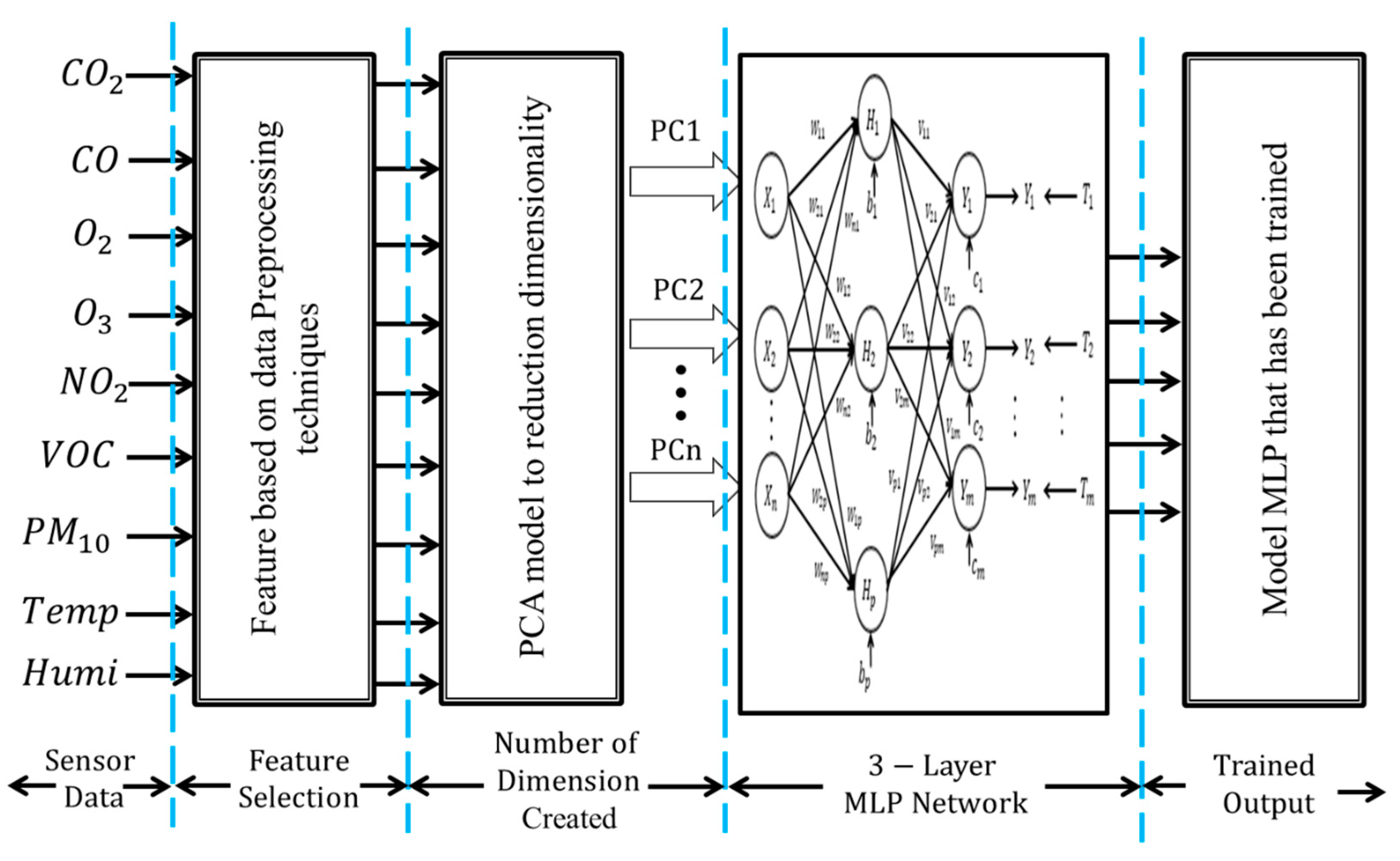
The example of one of the algorithms, such as the MLP model, along with its classification performance of six features is discussed in this section. For each of the features, a separate MLP model was formulated. Separate models need to be formulated as the aim of the research is to find the optimal classification accuracy for each feature. In order to identify the source affecting the IAQ, this study used the MLP, which consists of three layers: the input layer, hidden layer and output layer. As network architecture, a 3-layer perceptron model as shown in Figure 7 was used. The first input layer contains the input variables for the network, which is the data after the pre-processing technique. For the data set before PCA, the input layer contains nine neurons of IAQ parameters, which are CO₂, CO, O₃, NO₂, O₂, VOC, PM₁₀, temperature and humidity, while, for the data set after PCA, the input layer contains the dimensions for each feature after reduction. There is one hidden layer used and the numbers of hidden neurons were not fixed and were adjusted until the desired performance was achieved. The last layer of the model is the output layer, which consists of five target outputs that represent five types of sources of indoor air pollution, such as combustion activity, the presence of fragrances and so on. Sixty percent of all data is selected randomly to become the training set. A goal is set (in this case, a mean square error (MSE) of 0.0001 has been chosen as the goal) and the training dataset is trained until the desired MSE is obtained. MSE was used as the stopping criterion. Training was conducted until the MSE fell below 0.0001 or a maximum epoch limit of 1000 is reached. This is to ensure that the model is trained with minimum error iteration and not over-trained. The learning rate and momentum factor were chosen based on experimental analysis. The number of hidden neurons was adjusted by the network to achieve this goal. The testing tolerance of the neural network model was chosen as 0.1. This value is the maximum allowable tolerance level for the testing.

The detailed parameter for MLP training is given in

Table 9. Parameters for multilayer perceptron (MLP) training.

Training Parameter	Value
Sample Number of samples used for training: 2880 Number of samples used for testing: 1920	4800
Input	9
Hidden neurons	Flexible
Output neurons	5
Performance	MSE
Goal	0.0001
Learning rate	0.01
Momentum constant	0.5

. For example, to train the dataset (before PCA) for the condition of ambient air, the data from all 9 IAQ parameters become the neurons for the input layer. Randomly, 60% of each IAQ parameter was selected to be the training set (60% out of 960 data for ambient air). The training was conducted until the targeted MSE was reached or until a maximum epoch limit of 1000 was reached. This process was repeated with the other four conditions. In the end, the network would produce a model which was then tested against the 40% of the remaining data for all conditions (the testing set) in order to find the classification accuracy. The whole process was repeated again for different features. The model of the feature that gave the highest classification accuracy may be chosen to be embedded into the system after being compared to the model of other type of classifiers, such as KNN or LDA.

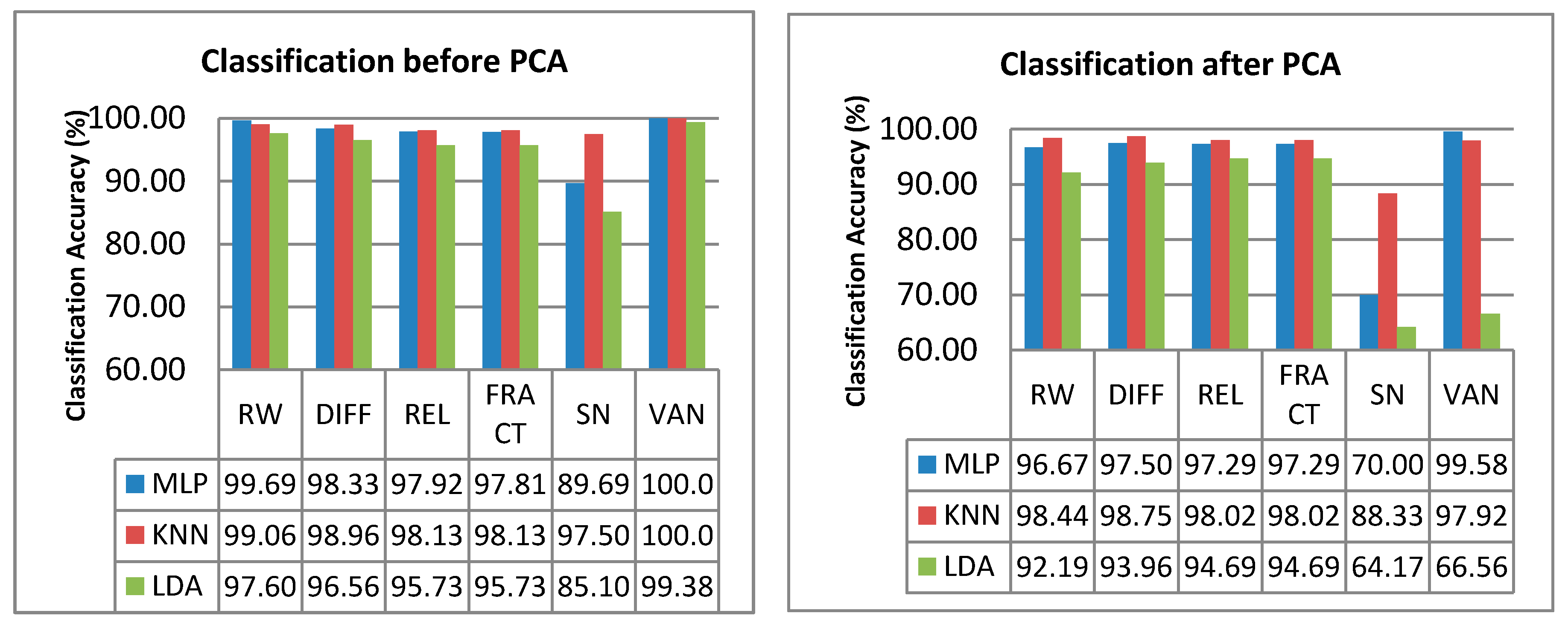
The classification performance of the MLP, KNN and LDA using the six features for the dataset before-PCA and after-PCA are shown in Figure 8. The PCA was performed because PCA is known to be able to increase the classification accuracy of certain datasets by reducing the number of variables, losing only a minimum of variability [46]. However, as shown in Figure 8, the classification rate for dataset after PCA is less than the classification rate before PCA for all features. This result is due to the information loss during PCA. According to [58], for datasets with very low complexity (few PCs), the relevant information has been excluded during the process of PCA, which resulted in a lower classification accuracy for datasets after PCA. The PCA could give a higher classification accuracy to datasets with very high complexity (many PCs), where the dataset before PCA does not only have relevant information, but also contains noise [59]. With the presence of noise, the classifier over-fits the training data and thus does not generalize well. Based on the explanation by [58], it can be seen that this study has a dataset with a very low complexity (only 9 PCs). Thus, the PCA process has excluded relevant information that could contribute to the high classification accuracy, which explains the lower classification accuracy for the dataset after PCA. Nevertheless, although the dataset after PCA (VAN feature) could not give 100% classification accuracy, it could classify 99.58% of the dataset using only two variables instead of nine variables needed for the dataset before PCA.

The validation in identifying pollutants by the proposed machine learning algorithm can be obtained by looking at the confusion matrix. A confusion matrix is a table that is often used to describe the performance of a classification model (or “classifier”) on a set of test data for which the true values are known. For example, in the case of the MLP classifier, the confusion matrix for the features giving the lowest and the highest classification accuracy are shown in

Table 10. Confusion matrix of multilayer perceptron (MLP) for sensor normalization (SN) after principal component analysis (PCA).

Actual	Predicted
	Sources of IAQ Pollutant	Ambient	Chemical	Food & Beverages	Fragrance	Human Activity	Confusion Level (%)
	Ambient	276	88	20	0	0	28.13
	Chemical	16	308	50	10	0	19.79
	Food & Beverages	0	16	280	84	4	27.08
	Fragrance	6	16	40	288	34	25.00
	Human Activity	4	12	60	116	192	50.00

and

Table 11. Confusion matrix of multilayer perceptron (MLP) for vector array normalization (VAN) before principal component analysis (PCA).

Actual	Predicted
	Sources of IAQ Pollutant	Ambient	Chemical	Food & Beverages	Fragrance	Human Activity	Confusion Level (%)
	Ambient	384	0	0	0	0	0
	Chemical	0	384	0	0	0	0
	Food & Beverages	0	0	384	0	0	0
	Fragrance	0	0	0	384	0	0
	Human Activity	0	0	0	0	384	0

. Rows and columns represent actual and predicted values, respectively. Table 10 shows the confusion matrix for feature SN (after PCA) as it gave the lowest confusion matrix. Based on the table, it can be observed that every condition contributes to the confusion level, with human activity having the highest confusion level at 50%. This means that MLP can classify only 50% of combustion activity correctly and it cannot classify the other 50% correctly as combustion activity.

Table 11 presents the confusion matrix for VAN (before PCA) which has the highest classification accuracy. Compared to the confusion matrix of SN in Table 10, MLP does not have any confusion in classifying all the five conditions. It means that it can classify all of the five conditions correctly. This confusion matrix validates the classification rate for VAN (before PCA), which is 100%.

The classification accuracy that has been achieved by this study is quite similar to the classification result achieved by a previous researcher [46]. They have developed a laboratory-made malodour sensing system, used to identify five typical sources of olfactive annoyance: printing houses, a paint shop in a coach building, wastewater treatment plant, urban waste composting facilities and a rendering plant. The researcher adopted various data pre-processing techniques, such as the VAN feature, which was also used in this study. Their results also show that the best classification results are obtained using a VAN feature with 100% classification accuracy. The objective of testing these three classifiers is to see which classifier gives the highest classification accuracy. Based on the results of the classifiers discussed before, there are four sets of classifiers with one feature (VAN before PCA) which gave 100% classification accuracy:

(1).

MLP-VAN feature before PCA (model 9-3-5),

(2).

MLP-VAN feature before PCA (model 9-9-5),

(3).

MLP-VAN feature before PCA (model 9-12-5), and

(4).

KNN-VAN feature before PCA (K factor is 2).

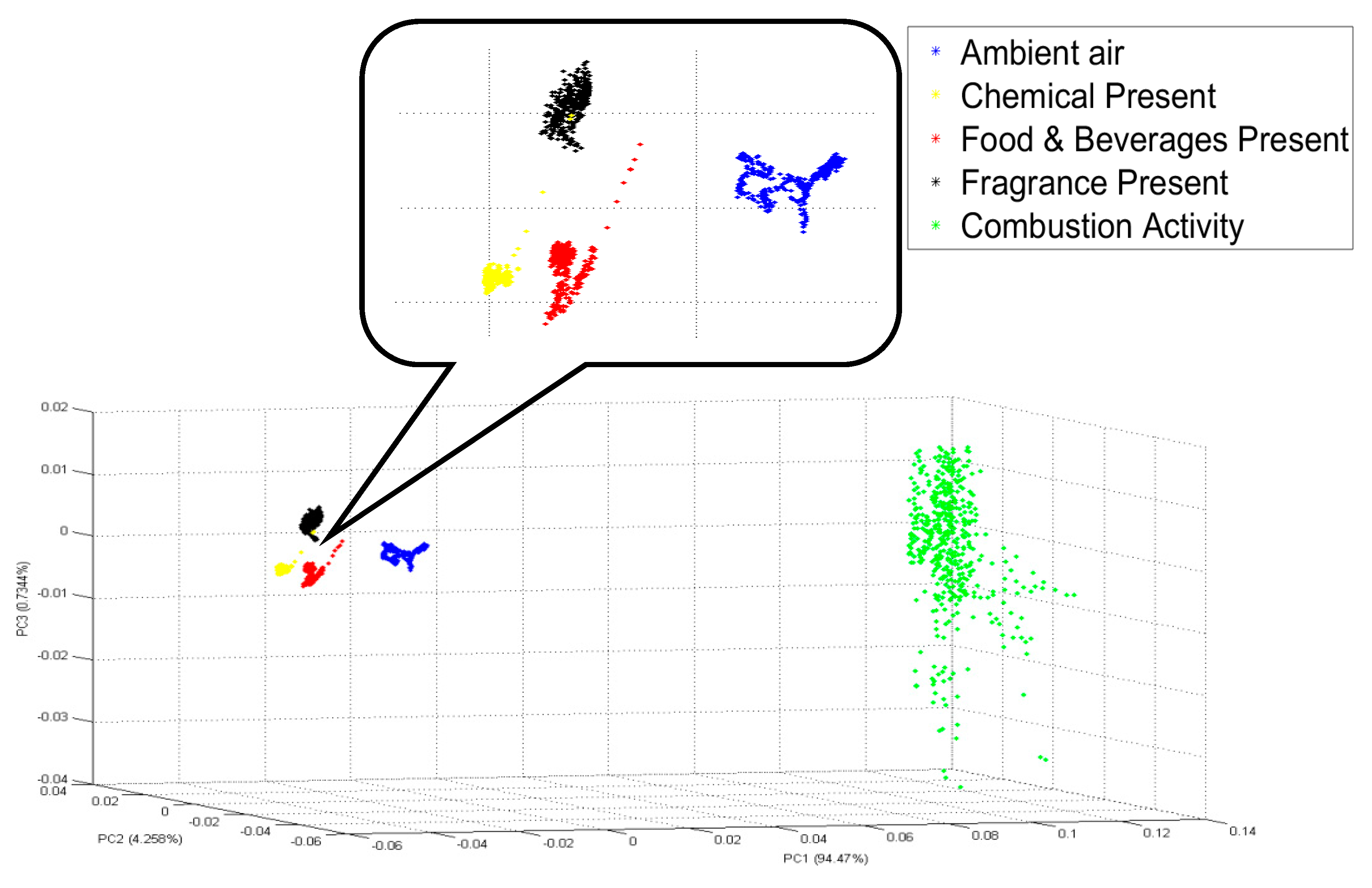
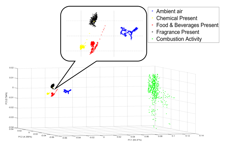
To prove that the VAN feature before PCA really gave 100% classification accuracy, another analysis has been done. The PCA visualization for the VAN feature before any dimensionality reduction is constructed in s 3D plot as shown in Figure 9. From Figure 9, it can be seen that none of the five conditions coincide with each other, and therefore they are mutually exclusive. After the feature has been identified, it is now time to choose between the two classifiers: MLP or KNN. This study chooses MLP with a model structure of 9-3-5 because it is easier to be embedded in the system. Model 9-3-5 only has three hidden variables, while the other two model structures have nine and 12 hidden variables. A model structure with fewer hidden variables has a less complicated formula and is therefore easy to be embedded. As far as KNN is concerned, KNN requires a large storage space in the system because it saves every data that it receives. MLP, on the other hand, does not require a large storage system. Due to these reasons, an MLP classifier is chosen for this study.

4.2. Classification of Multiple Sources of IAP

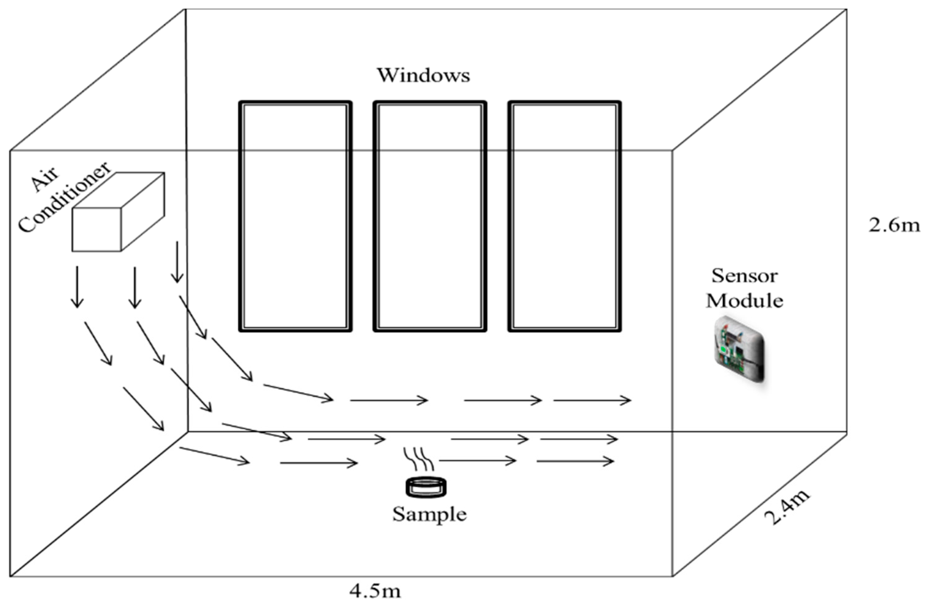
This section shows results for the classification of sources of IAP when multiple sources are present at the same time. Based on the previous result, the MLP classifier with a model structure of 9-3-5 was chosen for this analysis. To collect the related data for this analysis, an experiment that simulates the presence of multiple sources of IAP was conducted. A similar environment to the previous experiment of collecting a single source of IAP was maintained, where the sensor module was installed hanging up to the right of the wall with 1.1 m of height above the ground, and the temperature of the room was set to 22 °C. The data was collected for one day: between 9:00 a.m. and 11:30 a.m. 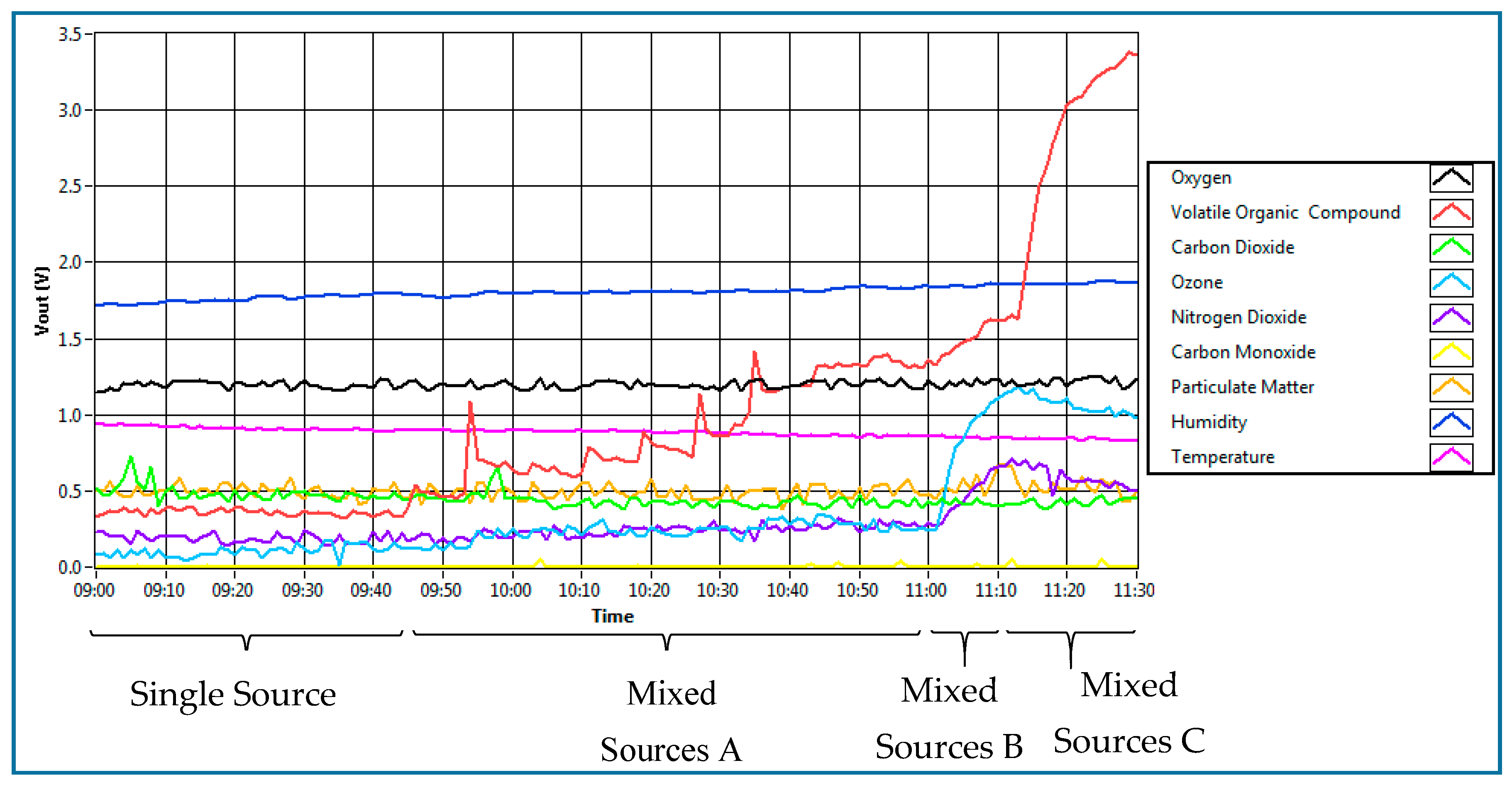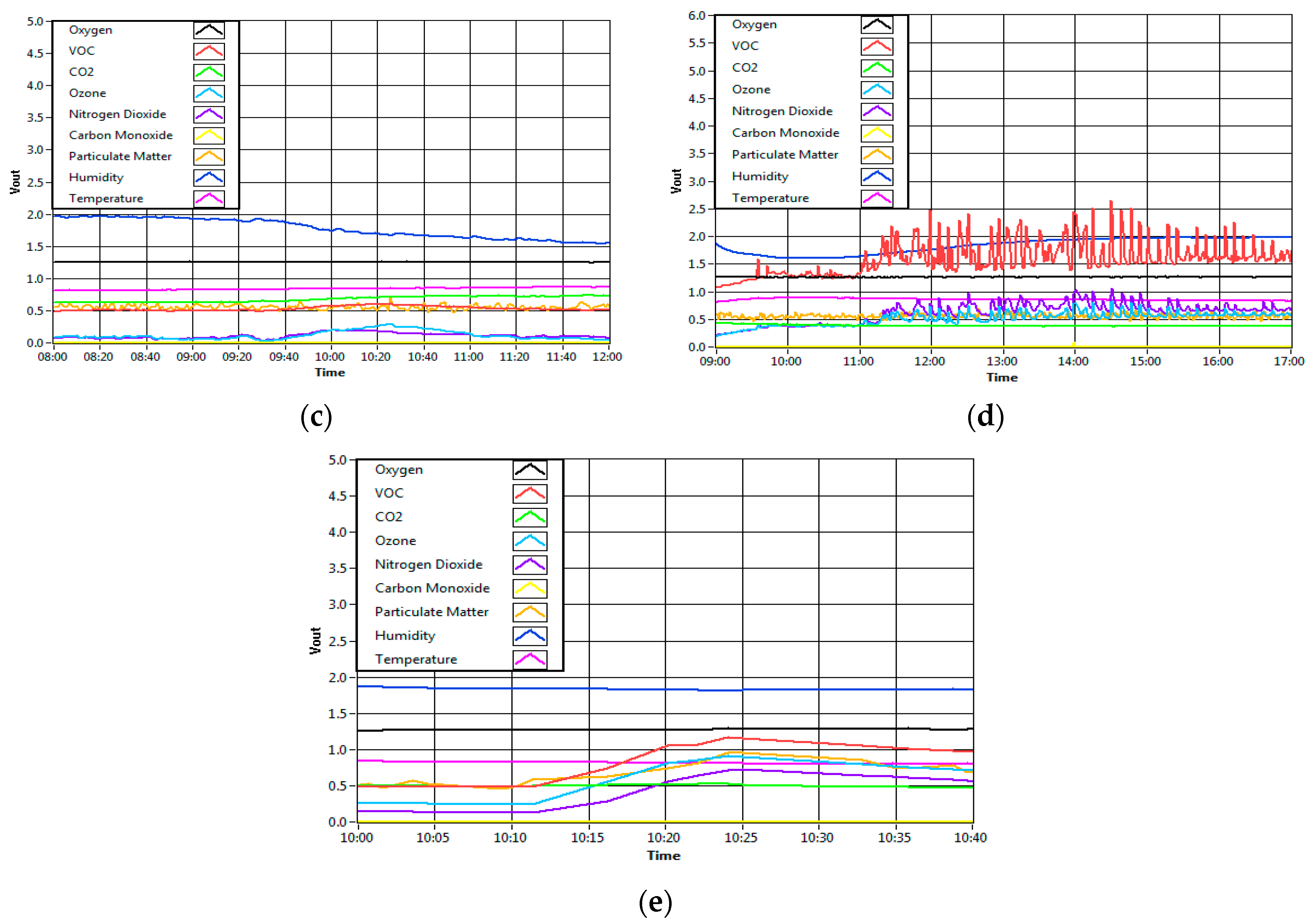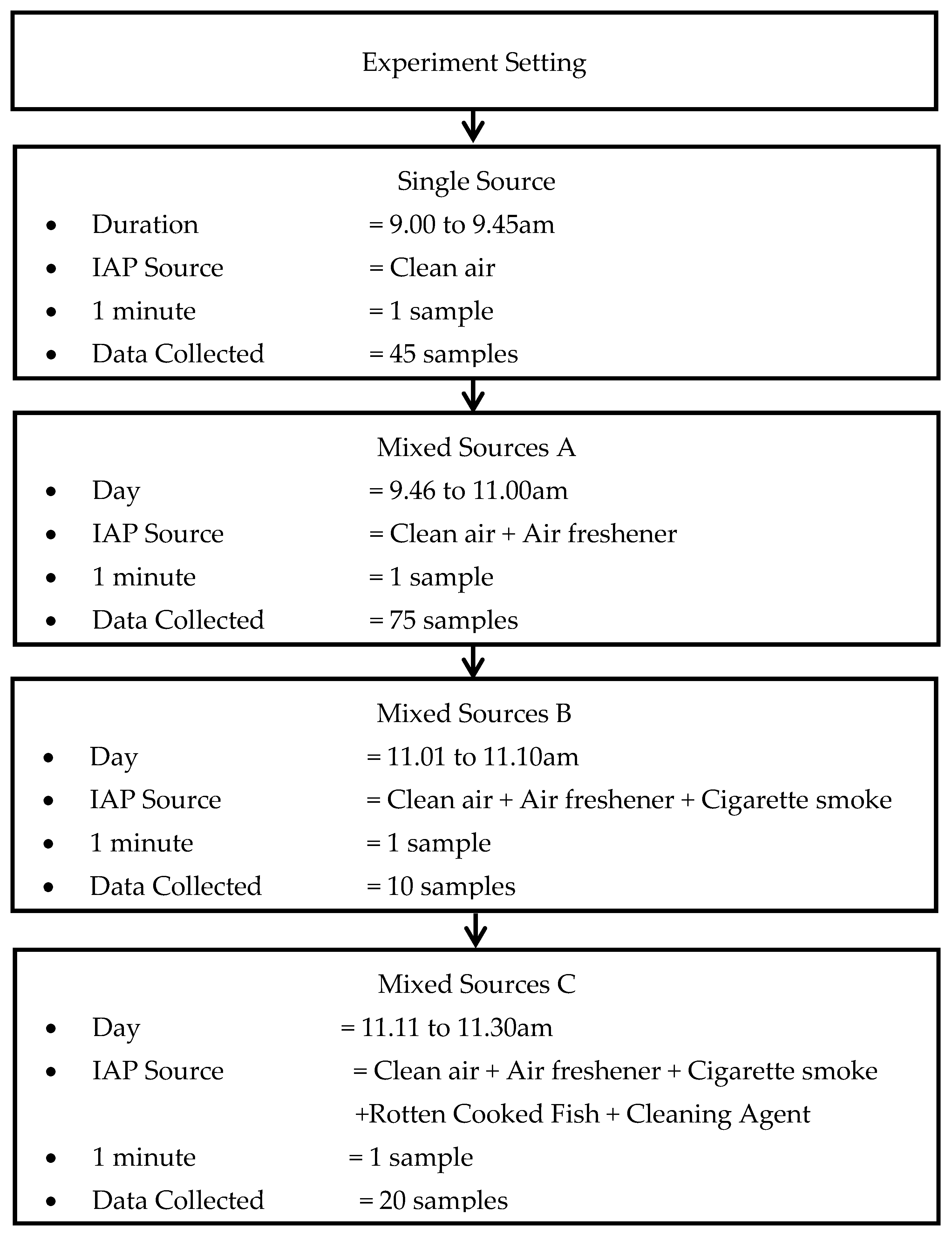Figure 10 shows the process of data collection for testing the system when all sources present in a room.

The experiment began with the first condition present, which was the ambient air. There were 45 samples collected for ambient air over 45 min duration. This environment was tagged as “single source”. Then, an automatic air freshener which released fragrance every 15 min was placed inside the room. This environment was conducted to simulate the presence of two sources: ambient air and fragrance. The air freshener was hung up on the wall with a height of 2 m from the floor and about 2 m from the sensing node. Total data collected for the air freshener was over 75 min. This environment is tagged as “mixed sources A”. After that, a person was asked to smoke in the room. This environment was conducted to simulate the presence of three sources of IAP: ambient air, fragrance and single cigarette smoke. That person smoked one cigarette at the centre of the room. One cigarette took 10 min, which contribute to a 10 min data sample. This environment was tagged as “mixed sources B”. Lastly, the other two sources of IAQ, which are food and beverages and chemical cleaning product, were added into the environment. These two sources of IAP were placed in the middle of the room for 20 min, which gave 20 samples. This environment was conducted to simulate the presence of all five sources of IAP. Although there was no person smoking in the room at this time, the presence of smoking can still be traced. The presence of smoking can be traced up to 30 min, as shown in Figure 10. This environment was tagged as “mixed sources C”.

Figure 11 shows the result of the sensor’s response for all situations as described above, from a single source up to five sources of IAP. It can be observed that the sensors react differently when additional sources of IAP are added into the room. The result of the classifier based on all environments is shows in

Table 12. Result of the classifier based on mixed sources.

Condition	Data Samples	Sources of IAQ Pollutant
		Ambient	Fragrance	Combustion Activity	Food & Beverages	Chemical	Unknown
Single source	45	45	0	0	0	0	0
Mixed sources A	75	7	68	0	0	0	0
Mixed sources B	10	0	1	7	0	0	2
Mixed sources C	20	0	0	1	2	7	10

. Based on the table, it can be observed that the system can precisely detect a single source (ambient) with 45 correct classifications out of 45 data samples. This means that the MLP classifier can classify an ambient environment at 100% classification rate. Similarly, when the fragrance is present in the condition of “mixed sources A”, the system correctly classifies the two mixed sources of IAQ. The system did not misclassify the sources as unknown sources. This result is as expected because the environment of fragrance mixed with the ambient air is similar to the presence of fragrance alone, and the system has already been trained with such an environment. On the other hand, the system could not classify two samples out of 10 samples as the available sources (ambient air, presence of fragrance and presence cigarette smoke) in the condition of “mixed sources B”. Nonetheless, the MLP classifier correctly classified the other eight samples as fragrance (one) and cigarette smoke (seven). The result is also as expected, because the presence of smoking was overpowering the presence of fragrance due to the high amount of gases produced during smoking as compared to the amount of gases produced by air freshener. Likewise, in the condition of “mixed sources C”, when all of the sources of IAP were mixed together in the room, the MLP classifier could correctly classify 50% of the samples as combustion activity (one), food and beverages (two) and presence of chemical (seven). The other 10 samples have been classified as unknown sources.

5. Conclusions

This study proposed an enhanced IAQMS which could recognize the pollutants by the utilized supervised machine learning algorithm that is widely used in data mining. With regards to pollutant recognition, it can be concluded that this IAQMS has successfully recognized five sources of indoor air pollution with a classification rate of 100 percent. These five sources of indoor air pollution—ambient air, combustion activity, presence of chemicals, presence of fragrances and presence of food and beverages—are successfully classified by MLP and KNN using the VAN before PCA feature. To prove that all the five sources of indoor air pollution are mutually exclusive, a 3-D graph has been attached, as shown in Section 4. Three classifiers have been tested to choose for the best classifier: MLP, KNN and LDA. In the end, the MLP classifier with a model structure of 9-3-5 has been chosen to be embedded into the IAQMS because it is more suitable to be embedded in the system. A model structure with fewer hidden variables has a less complicated formula and is therefore easy to embed. KNN requires a large storage space in the system because it saves every data that it receives. MLP, on the other hand, does not require a large storage system. Due to these reasons, the MLP classifier is chosen for this project. The system has also been tested with multiple sources of IAP presented together. The result shows that the system is able to classify when single and two mixed sources are presented together; however, when more than two sources of IAP are presented at the same period, the system will classify the sources as ‘unknown’ because the system cannot recognize the input of the new pattern. Hence, the classification accuracy falls dramatically. Future research should consider expanding the sources of indoor air pollution to include more sources of indoor air pollution. In addition, the proxy for each condition could also be added to include more activity and to test the efficiency of IAQ that can detect more sources of IAP such as furniture (wood, plastic), building materials (plaster, insulation), and coatings (carpeting, painting). In order to sense mixed sources, more sensitive sensors might provide more insight; more sensitive sensors with the ability to distinguish the different sources need to used. Furthermore, the system can also be trained with two or more mixed sources, for example, mixing between air freshener with smoking activity and the presence of food and beverages. For this study, a neural network (NN) used to classify the sources of indoor air pollution is embedded into the IAQMS only. Therefore, this study would like to suggest that the NN should be embedded onto the microcontroller for future research. If the classifier is embedded onto the microcontroller, the IAQMS could operate as a stand-alone device, which would enable the IAQMS to send an alert to users (via short massage system (SMS)) if the air quality level in the observed room changed to a “bad” or “hazardous” level.

References

1. Environmental Protection Agency (EPA). Buildings and Their Impact on the Environment: A Statistical Summary; Environmental Protection Agency Green Building Workgroup: Washington, DC, USA, 2009. Available online: http://www.epa.gov/greenbuilding/pubs/gbstatpdf (accessed on 26 November 2014).
2. Reffat, R.M.; Harkness, E.L. Environmental comfort criteria: Weighting and integration. J. Perform. Constr. Facil. 2001, 15, 104–108. [Google Scholar] [CrossRef]
3. Batterman, S.; Burge, H. HVAC systems as emission sources affecting indoor air quality: A critical review. HVAC&R Res. 1995, 1, 61–78. [Google Scholar]
4. World Health Organization (WHO). Indoor Air Quality Guidelines: Household Fuel Combustion; WHO: Geneva, Switzerland, 2014. [Google Scholar]
5. Borkar, C. Development of Wireless Sensor Network System for Indoor Air Quality Monitoring. Master’s Thesis, University of North Texas, Denton, TX, USA, 2012. [Google Scholar]
6. Centers for Disease Control and Prevention (CDC). Indoor Environmental Quality: Chemicals and Odors; CDC: Atlanta, GA, USA, 2014. Available online: http://www.cdc.gov/niosh/topics/indoorenv/chemicalsodors.html. (accessed on 13 December 2014).
7. Mumyakmaz, B.; Karabacak, K. An E-Nose-based indoor air quality monitoring system: Prediction of combustible. Turk. J. Electr. Eng. Comput. Sci. 2015, 2, 1–12. [Google Scholar]
8. Sait, C.S. The Development of the Indoor Air Pollution Index for Office Buildings. Ph.D. Thesis, Illinois Institute of Technology, Chicago, IL, USA, 2001. [Google Scholar]
9. Wasana, T. A Validation Method for the Development of Carbon Monoxide Wireless Sensor for Ambient Air Monitoring. Master’s Thesis, University of Cincinnati, Cincinnati, OH, USA, 2007. [Google Scholar]
10. Department of Occupational Safety and Health (DOSH). Industry Code of Practice On Indoor Air Quality; DOSH: Putrajaya, Malaysia, 2010.
11. Postolache, O.A.; Pereira, J.M.D.; Girao, P.M.B.S. Smart sensors network for air quality monitoring applications. IEEE Trans. Instrum. Meas. Trans. Instrum. Meas. 2009, 58, 3253–3262. [Google Scholar] [CrossRef]
12. American Society of Heating Refrigerating and Air-Conditioning Engineers (ASHRAE). 2009 Ashrae Handbook: Fundamentals, I-P ed.; ASHRAE: Atlanta, GA, USA, 2009. [Google Scholar]
13. Indoor Air Quality Management Group (IAQMG). Guidance Notes for the Management of Indoor Air Quality in Offices and Public Places; IAQMG: Hong Kong, China, 2003.
14. Rahul, R. An Embedded Real-Time Environment Monitoring System. Master’s Thesis, University of Texas at Arlington, Arlington, MA, USA, 2002. [Google Scholar]
15. Thad, G. Indoor Environmental Quality; CRC Press: Boca Raton, FL, USA, 2001. [Google Scholar]
16. Yau, Y.H.; Chew, B.T.; Saifullah, A.Z. Studies on the indoor air quality of Pharmaceutical Laboratories in Malaysia. Int. J. Sustain. Built Environ. 2012, 1, 110–124. [Google Scholar] [CrossRef]
17. Environmental Protection Agency (EPA). Indoor Air: An Introduction to Indoor Air Quality (IAQ); EPA: Washington, DC, USA, 2014. Available online: http://www.epa.gov/iaq/ia-intro.html (accessed on 12 January 2015).
18. Maroni, M.; Seifert, B.; Lindwall, T. Indoor Air Quality: A Comprehensive Reference Book; Elsevier: New York, NY, USA, 1995. [Google Scholar]
19. Mohave, L. Indoor air quality and health. In Proceedings of the Healthy Buildings 2000, Espoo, Finland, 6–10 August 2000. [Google Scholar]
20. Environmental Protection Agency (EPA). Care for Your Air: A Guide to Indoor Air Quality; EPA: Washington, DC, USA, 2008.
21. Capelli, L.; Sironi, S.; del Rosso, R. Electronic noses for environmental monitoring applications. Sensors 2014, 14, 19979–20007. [Google Scholar] [CrossRef] [PubMed] [Green Version]
22. Dentoni, L.; Capelli, L.; Sironi, S.; del Rosso, R.; Zanetti, S.; della Torre, M. Development of an electronic nose for environmental odour monitoring. Sensors 2012, 12, 14363–14381. [Google Scholar] [CrossRef] [PubMed]
23. Nicolas, J.; Romain, A.C.; Wiertz, V.; Maternova, J.; André, P. Using the classification model of an electronic nose to assign unknown malodours to environmental sources and to monitor them continuously. Sens. Actuators B Chem. 2000, 69, 366–371. [Google Scholar] [CrossRef]
24. Sironi, S.; Capelli, L.; Céntola, P.; del Rosso, R.; Grande, M.I. Continuous monitoring of odours from a composting plant using electronic noses. Waste Manag. 2007, 27, 389–397. [Google Scholar] [CrossRef] [PubMed]
25. Sohn, J.H.; Pioggia, G.; Craig, I.P.; Stuetz, R.M.; Atzeni, M.G. Identifying major contributing sources to odour annoyance using a non-specific gas sensor array. Biosyst. Eng. 2009, 102, 305–312. [Google Scholar] [CrossRef]
26. Archie, L.W. Prediction Of Odor Pleasantness Using Electronic Nose Technology and Artificial Neural Networks. Ph.D. Thesis, Pennsylvania State University, State College, PA, USA, 2006. [Google Scholar]
27. Kim, D.K.; Roh, Y.W.; Hong, K.S. A method of multiple odors detection and recognition. In Proceedings of the International Conference on Human-Computer Interaction, Orlando, FL, USA, 9–14 July 2011; Volume 6762, pp. 464–473. [Google Scholar]
28. Loutfi, A.; Coradeschi, S. Odor recognition for intelligent systems. IEEE Intell. Syst. 2008, 23, 41–48. [Google Scholar] [CrossRef]
29. Tong, Z.; Chen, Y.; Malkawi, A.; Adamkiewicz, G.; Spengler, J.D. Quantifying the impact of traffic-related air pollution on the indoor air quality of a naturally ventilated building. Environ. Int. 2016. [Google Scholar] [CrossRef] [PubMed]
30. Tong, Z.; Yang, B.; Hopke, P.K.; Zhang, K.M. Microenvironmental air quality impact of a commercial-scale biomass heating system. Environ. Pollut. 2017, 220, 1112–1120. [Google Scholar] [CrossRef] [PubMed]
31. OSHA. Indoor Air Quality in Commercial and Institutional Building; OSHA: Washington, DC, USA, 2011.
32. Department of Safety and Health (DOSH). DOSH Profile; Department of Safety and Health, Ministry of Human Resources: Putrajaya, Malaysia, 2014.
33. Figaro. Technical Information For Air Quality Control Sensors; Figaro: Osaka, Japan, 2001. [Google Scholar]
34. Figaro. TGS 2602—For the Detection of Air Contaminants; Figaro: Osaka, Japan, 2005. [Google Scholar]
35. Saad, S.M.; Andrew, A.M.; Shakaff, A.Y.M.; Saad, A.R.M.; Kamarudin, A.M.Y.; Zakaria, A. Classifying sources influencing indoor air quality (IAQ) using artificial neural network (ANN). Sensors 2015, 15, 11665–11684. [Google Scholar] [CrossRef] [PubMed]
36. Aeroqual. Series-200-300-500-Portable-Monitor-User-Guide-11–14; Aeroqual: Auckland, New Zealand, 2014. [Google Scholar]
37. Invernizzi, R.B.G.; Ruprecht, A.; Mazza, R.; Rossetti, E.; Sasco, A.; Nardini, S. Particulate matter from tobacco versus diesel car exhaust: An educational perspective. Tob. Control 2004, 13, 219–221. [Google Scholar] [CrossRef] [PubMed]
38. Meena, K. Indoor Air Pollution: Sources, Health Effects and Mitigation Strategies. In The Encylopedia of Earth; Environmental Information Coalition: Washington, DC, USA, 2009; Available online: http://editors.eol.org/eoearth/wiki/Indoor_air_quality_(IAQ) (accessed on 31 January 2015).
39. Loomis, D.; Grosse, Y.; Lauby-Secretan, B.; El Ghissassi, F.; Bouvard, V.; Benbrahim-Tallaa, L.; Guha, N.; Baan, R.; Mattock, H.; Straif, K.; et al. The carcinogenicity of outdoor air pollution. Lancet Oncol. 2013, 14, 1262–1263. [Google Scholar] [CrossRef]
40. Andrew, A.M.; Zakaria, A.; Saad, S.M.; Shakaff, A.Y.M. Multi-stage feature selection based intelligent classifier for classification of incipient stage fire in building. Sensors 2016, 16, 31. [Google Scholar] [CrossRef] [PubMed]
41. Bahram, G.K. On Using Artificial Neural Networks and Genetic Algorithms to Optimize Performance of an Electronic Nose. Ph.D. Thesis, North Carolina State University, Raleigh, NC, USA, 1996. [Google Scholar]
42. Distante, C.; Leo, M.; Siciliano, P.; Persaud, K.C. On the study of feature extraction methods for an electronic nose. Sens. Actuators B Chem. 2002, 87, 274–288. [Google Scholar] [CrossRef]
43. Gutierrez-Osuna, R.; Nagle, H.T. A method for evaluating data-preprocessing techniques for odor classification with an array of gas sensors. IEEE Trans. Syst. Man Cybern. B Cybern. 1999, 29, 626–632. [Google Scholar] [CrossRef] [PubMed]
44. Gutierrez-Osuna, R. Pattern analysis for machine olfaction: A review. IEEE Sens. J. 2002, 2, 189–202. [Google Scholar] [CrossRef]
45. Bahraminejad, B.; Basri, S.; Isa, M.; Hambli, Z. Real-time gas identification by analyzing the transient response of capillary-attached conductive gas sensor. Sensors 2010, 10, 5359–5377. [Google Scholar] [CrossRef] [PubMed]
46. Romain, A.C.; Nicolas, J.; Wiertz, V.; Maternova, J.; Andre, P. Use of a simple tin oxide sensor array to identify five malodours collected in the field. Sens. Actuators B Chem. 2000, 62, 73–79. [Google Scholar] [CrossRef]
47. Gardner, J.W.; Bartlett, P.N. A brief history of electronic noses. Sens. Actuators B Chem. 1994, 18, 210–211. [Google Scholar] [CrossRef]
48. Scott, S.M.; James, D.; Ali, Z. Data analysis for electronic nose systems. Microchim. Acta 2006, 156, 183–207. [Google Scholar] [CrossRef]
49. Kim, Y.; Kim, I.; Kim, J.; Yoo, C. Real-time multivariate monitoring and diagnosis of air pollutants in a subway station. In Proceedings of the International Conference on Control, Automation and Systems, Seoul, Korea, 14–17 October 2008; pp. 2610–2615. [Google Scholar]
50. Hidayat, W.; Shakaff, A.Y.; Ahmad, M.N.; Adom, A.H. Classification of agarwood oil using an electronic nose. Sensors 2010, 10, 4675–4685. [Google Scholar] [CrossRef] [PubMed]
51. Kim, E.; Lee, S.; Kim, J.H.; Kim, C.; Byun, Y.T.; Kim, H.S.; Lee, T. Pattern recognition for selective odor detection with gas sensor arrays. Sensors 2012, 12, 16262–16273. [Google Scholar] [CrossRef] [PubMed]
52. Yingjie, Z. Portable Electronic Nose System for Detecting Volatile Organic Compounds. Master’s Thesis, University of Massachusetts Lowell, Lowell, MA, USA, 2012. [Google Scholar]
53. Kaiser, H. The application of electronic computers to factor analysis. Educ. Psychol. Meas. 1960, 20, 141–151. [Google Scholar] [CrossRef]
54. Kotsiantis, S.B.; Zaharakis, I.D.; Pintelas, P.E. Machine learning: A review of classification and combining techniques. Artif. Intell. Rev. 2006, 26, 159–190. [Google Scholar] [CrossRef]
55. Schiffman, S.S.; Wyrick, D.W.; Nagle, H.T. Effectiveness of an Electronic Nose for Monitoring Bacterial and Fungal Growth; CRC Press: Boca Raton, FL, USA, 2001. [Google Scholar]
56. Yolanda, G.M.; Oliveros, C.; Perez, P.; Carmelo, G.; Bernardo, M.C. Electronic nose based on metal oxide semiconductor sensors and pattern recognition techniques: Characterisation of vegetable oils. Anal. Chim. Acta 2001, 449, 69–80. [Google Scholar]
57. Mamat, M.; Samad, S.A.; Hannan, M.A. An electronic nose for reliable measurement and correct classification of beverages. Sensors 2011, 11, 6435–6453. [Google Scholar] [CrossRef] [PubMed]
58. Trevor, H.; Robert, T.; Jerome, F. The Elements of Statistical Learning: Data Mining, Inference and Prediction; Springer: Berlin, Germany, 2009; Volume 2. [Google Scholar]
59. Howley, T.; Madden, M.G.; Connell, M.O.; Ryder, A.G. The Effect of principal component analysis on machine learning accuracy with high dimensional spectral data. Knowl. Based Syst. 2006, 19, 363–370. [Google Scholar] [CrossRef]
Figure 1. System architecture for real-time indoor air quality (IAQ) monitoring.
Applsci 07 00823 g001
Figure 2. (a) NO2 data; (b) Temperature data; (c) Humidity data.
Applsci 07 00823 g002aApplsci 07 00823 g002b
Figure 3. Room setup for the experiment.
Applsci 07 00823 g003
Figure 4. (a) Ambient environment; (b) Chemical presence; (c) Food and beverages; (d) Fragrance presence; and (e) Combustion activity.
Applsci 07 00823 g004aApplsci 07 00823 g004b
Figure 5. Steps in pattern recognition.
Applsci 07 00823 g005
Figure 6. Typical sensor response.
Applsci 07 00823 g006
Figure 7. Network architecture of the multilayer perceptron (MLP) model.
Applsci 07 00823 g007
Figure 8. Classification performance for the before- principal component analysis (PCA) and after- principal component analysis (PCA) dataset.
Applsci 07 00823 g008
Figure 9. 3D plot of PCA visualization for the VAN feature.
Applsci 07 00823 g009
Figure 10. Data collection procedures for multiple sources present.
Applsci 07 00823 g010
Figure 11. Sensor’s response when additional sources of IAP are present.
Applsci 07 00823 g011