Global Analysis for an HIV Infection Model with CTL Immune Response and Infected Cells in Eclipse Phase


1
Laboratory of Mathematics and Applications, Faculty of Sciences and Technologies, University Hassan II of Casablanca, P.O. Box 146, Mohammedia 20650, Morocco
2
School of Mathematical and Statistical Sciences, Arizona State University, Tempe, AZ 85287, USA
*
Author to whom correspondence should be addressed.
Appl. Sci. 2017, 7(8), 861; https://doi.org/10.3390/app7080861
Submission received: 27 July 2017
/
Revised: 12 August 2017
/
Accepted: 17 August 2017
/
Published: 21 August 2017
Abstract
:A modified mathematical model describing the human immunodeficiency virus (HIV) pathogenesis with cytotoxic T-lymphocytes (CTL) and infected cells in eclipse phase is presented and studied in this paper. The model under consideration also includes a saturated rate describing viral infection. First, the positivity and boundedness of solutions for nonnegative initial data are proved. Next, the global stability of the disease free steady state and the endemic steady states are established depending on the basic reproduction number and the CTL immune response reproduction number . Moreover, numerical simulations are performed in order to show the numerical stability for each steady state and to support our theoretical findings. Our model based findings suggest that system immunity represented by CTL may control viral replication and reduce the infection.
1. Introduction
Human immunodeficiency virus (HIV) is known as a pathogen causing the acquired immunodeficiency syndrome (AIDS), which is the end-stage of the infection. After that, the immune system fails to play its life-sustaining role [1,2]. Indeed, it is well known that the cellular immune responses play an indispensable role during the HIV viral infection, especially in people known as elite controllers who are infected by HIV but maintain a normal CD4 count for many years and remain asymptomatic or have a very delayed disease progression over the course of their HIV infection [3,4].
The basic viral infection model with CTLs immune was first studied in [5] and its global stability was studied in [6,7]. A prevailing theory suggests that CTL cells are responsible for the sudden decrease HIV virus load and the subsequent quasi-steady state level of the viral load after a sharp increase during the primary infection phase [8,9,10,11]. In [12], the authors consider the interaction between CTL, viruses and macrophages and study the global stability in a model with a mass action infection term. With a saturated infection term, the same mathematical question was tackled in [13] with a model consisting of four ordinary differential equations with a Beddington–DeAngelis infection term.
More recently, the model describing the interaction between the HIV viruses, CD4 T cells, infected cells with a standard incidence rate function describing saturated viral infection is formulated and studied in [14]. The authors study the local and global stability of the endemic states and illustrate that their model can fit well with some clinical HIV infection data sets. In this paper, we extend their work by incorporating the cytotoxic T lymphocytes (CTL) immune response. The dynamics of HIV infection with CTL response that we consider is given by the following nonlinear system of differential equations:
with the initial conditions , , , and .
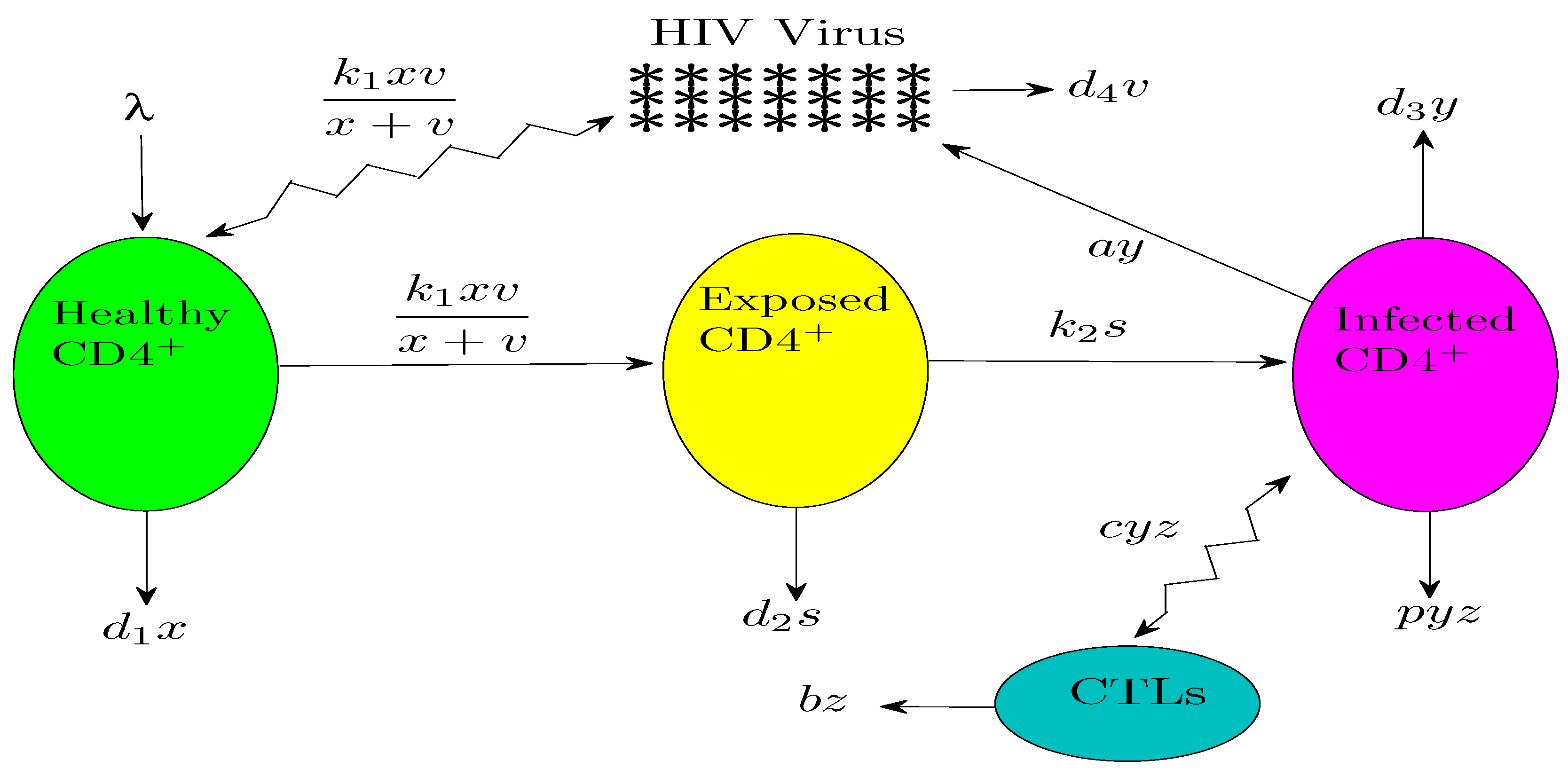
In this model, x, y, s, v and z denote the concentration of uninfected cells, infected cells, exposed cells, free virus and CTL cells, respectively. Susceptible host cells CD4 T cells are produced at a rate , die at a rate and become infected by virus at a rate . Exposed cells die at a rate and become infected at a rate of . Infected cells increase at rate and die at rate and are killed by the CTL response at a rate . Free virus is produced by infected cells at a rate and decays at a rate . Finally, CTLs expand in response to viral antigen derived from infected cells at a rate and decay in the absence of antigenic stimulation at a rate . Note that this model (1) employs the more realistic standard incidence rate function as in [14,15], which better describes the rate of viral infection. The schematic representing the viral dynamics of the problem under consideration is illustrated in Figure 1.
The rest of the paper is organized as follows. In Section 2, we study the positivity and boundedness of solutions. We present the steady states and give a local stability result in Section 3. Section 4 is dedicated to the global stability results. Numerical simulations are performed in Section 5 and we conclude the paper in the last section.
2. Mathematical Analysis of the HIV Model
2.1. Existence and Local Stability
For the problems deal with cell population evolution, the cell densities should remain non-negative and bounded. In this section, we will establish the positivity and boundedness of solutions of the model (1). First of all, for biological reasons, the parameters , , , and must be larger than or equal to 0. Hence, we have the following result:
Proposition 1.
For any non-negative initial conditions , system (1) has a unique solution. Moreover, this solution is non-negative and bounded for all .
Proof.
The proof is given in Appendix A. ☐
Moreover, system (1) has an infection-free equilibrium , corresponding to the maximal level of healthy CD4 T-cells. The basic reproduction number of our problem is given as follows:
where is the proportion of exposed cells to become productively infected cells, is the number of free virus production by an infected cell and is the average life of virus. From a biological point of view, stands for the average number of secondary infections generated by one infected cell when all cells are susceptibles. Depending on the value of this basic reproduction number ; in other words, depending on these three biological proportions, we will study the stability of the free-endemic and the endemic equilibria.
In addition to the disease free equilibrium, system (1) has three endemic equilibria. The first of them is , where
The second endemic steady state is , where
The third endemic steady state is , where
with .
The last endemic steady-state will not be taken under consideration since , which is not possible biologically. On the other hand, from the components of , it is clear that, when , this endemic point exists. In what follows, we will make use of the following CTL immune response reproduction number to classify the model system dynamics
depending on the value of this CTL immune reproduction number ; in other words, depending on and the parameters describing the effectiveness of CTL like c and b, we will study the stability of the endemic equilibria.
First, observe that the second endemic state exists when . This endemic state is also called an interior equilibrium.
We explain the existence of this endemic equilibrium as follows. We recall first that, in this state, both of the free viruses and CTL cells are present. Assume that , in the total absence of CTL immune response, the infected cell load per unit time is . Via the five equations of model (1), CTL cells reproduced due to infected cells stimulating per unit time is . The CTL load during the lifespan of a CTL cell is . If , we will have the existence of the endemic equilibrium .
The local stability result of the disease-free equilibrium is given as follows.
Proposition 2.
The disease-free equilibrium, , is locally asymptotically stable for .
Proof.
The proof is given in Appendix A. ☐
The local stability of the other steady states is quite similar to the first one. Hence, the rest of the work will be devoted only to the global stability analysis of the problem under consideration.
2.2. Global Stability Results
This subsection deals with the global stability analysis of the disease-free and the endemic equilibria. Our approach involves the construction of appropriate Lyapunov functions. First, we have the following global stability result of the disease-free equilibrium.
Proposition 3.
If , then the endemic point is globally stable.
Proof.
The proof is given in Appendix B. ☐
For the global stability result of the endemic equilibrium , we have the following.
Proposition 4.
If and , then the endemic point is globally stable.
Proof.
The proof is given in Appendix B. ☐
Finally, the global stability result concerning the last endemic point is given as follows.
Proposition 5.
If and , then the endemic point is globally stable.
Proof.
The proof is given in Appendix B. ☐
3. Numerical Results and Simulations
In order to perform the numerical simulations, system (1.1) will be solved numerically using the fourth order Runge–Kutta iterative scheme. The parameter values or ranges used are presented in Table 1.
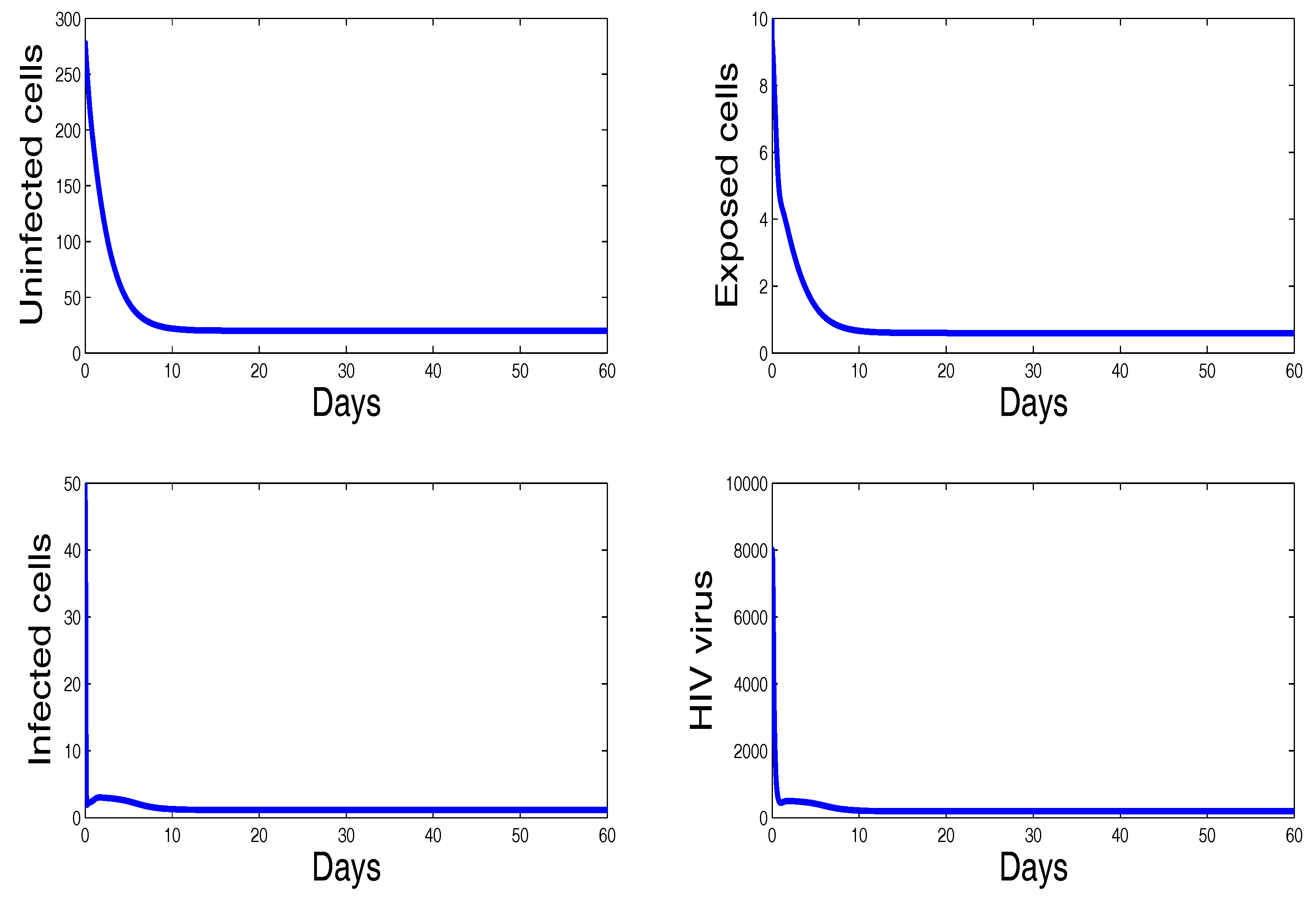
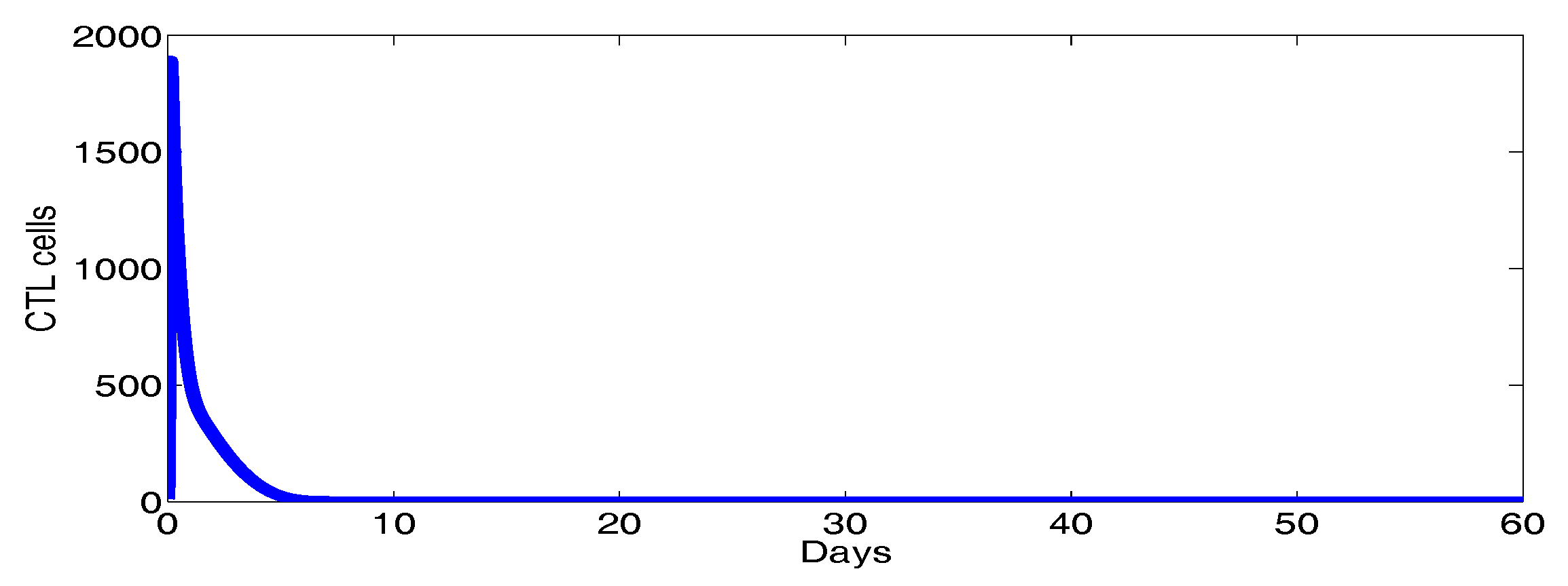
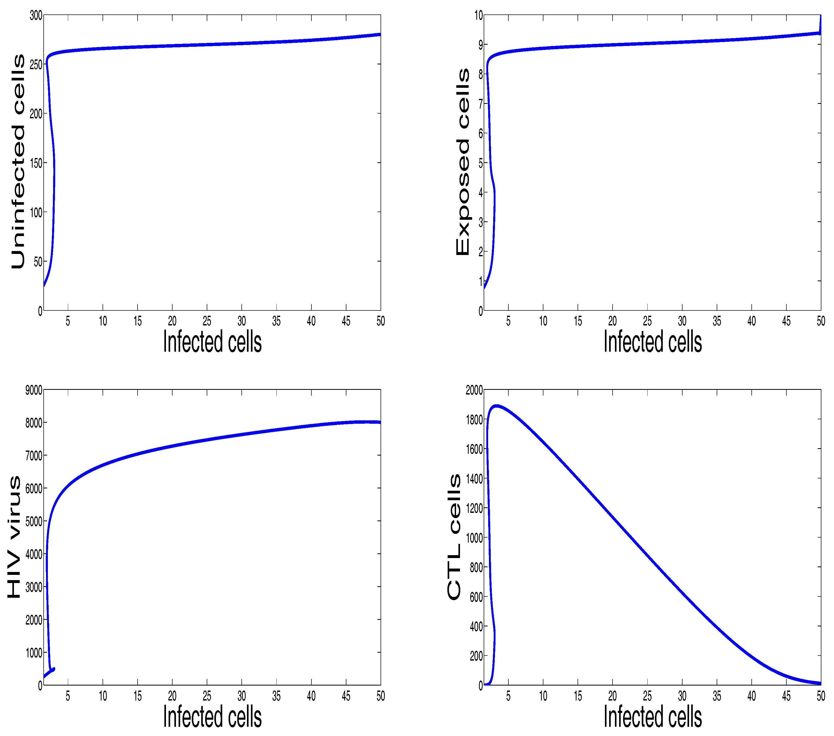
Figure 2 shows the behavior of infection during the first 60 days. For the parameters used in this figure, the basic reproduction number is ; we clearly see that the solutions of the system converge to the disease-free equilibrium point . This numerical result is consistent with the theoretical result concerning the stability of . In addition, the plots showing the stability of this disease-free point in phase plane are given in Figure 3.
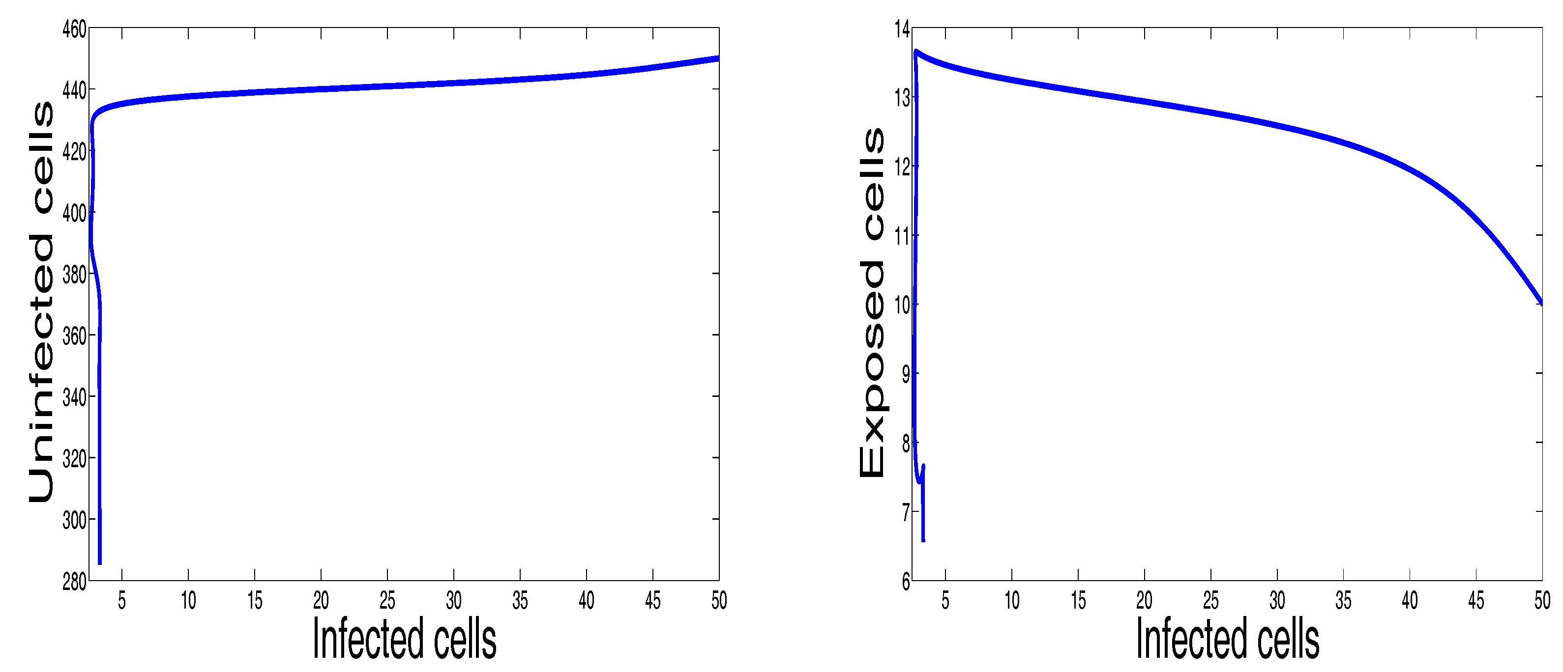
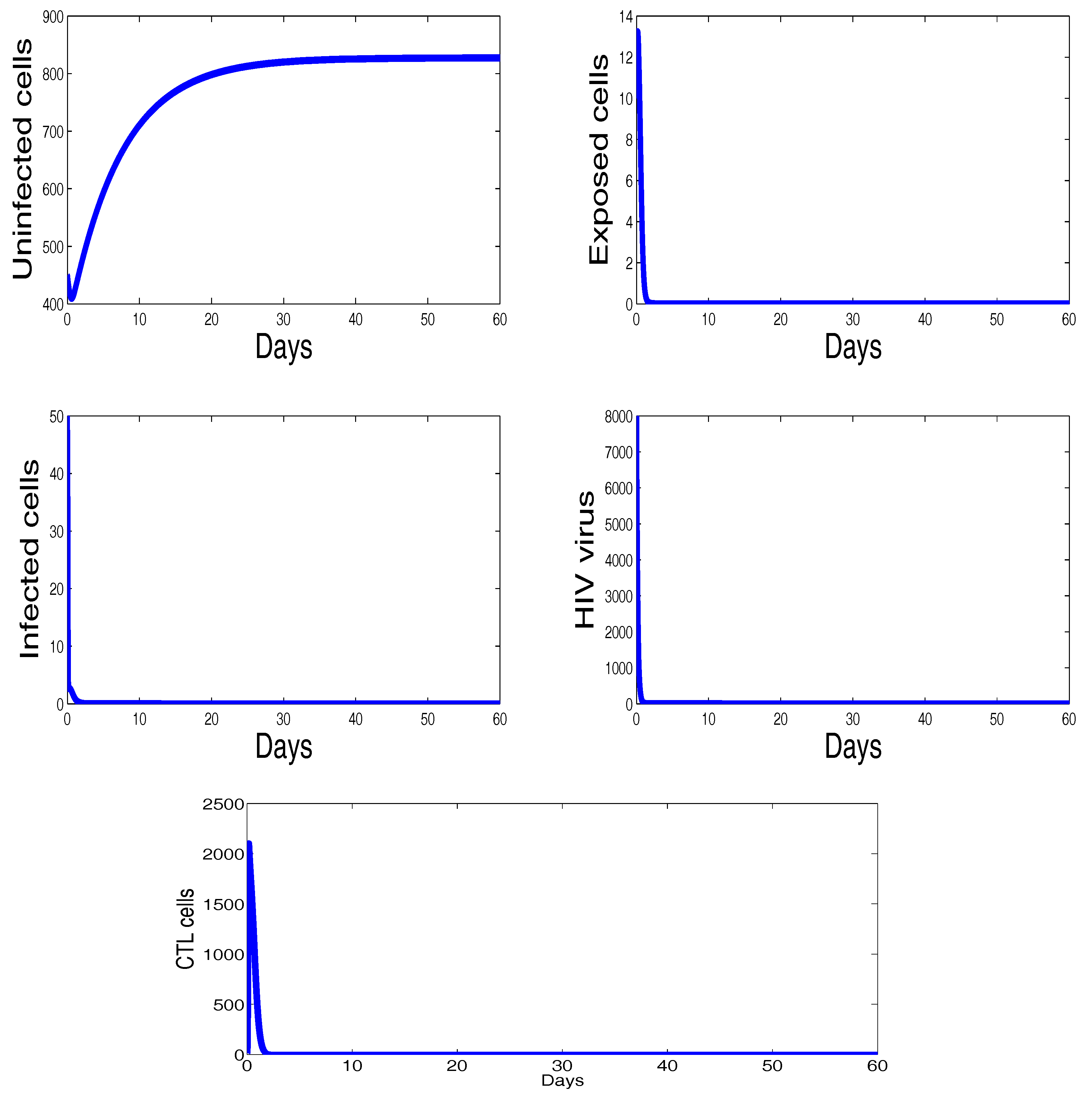
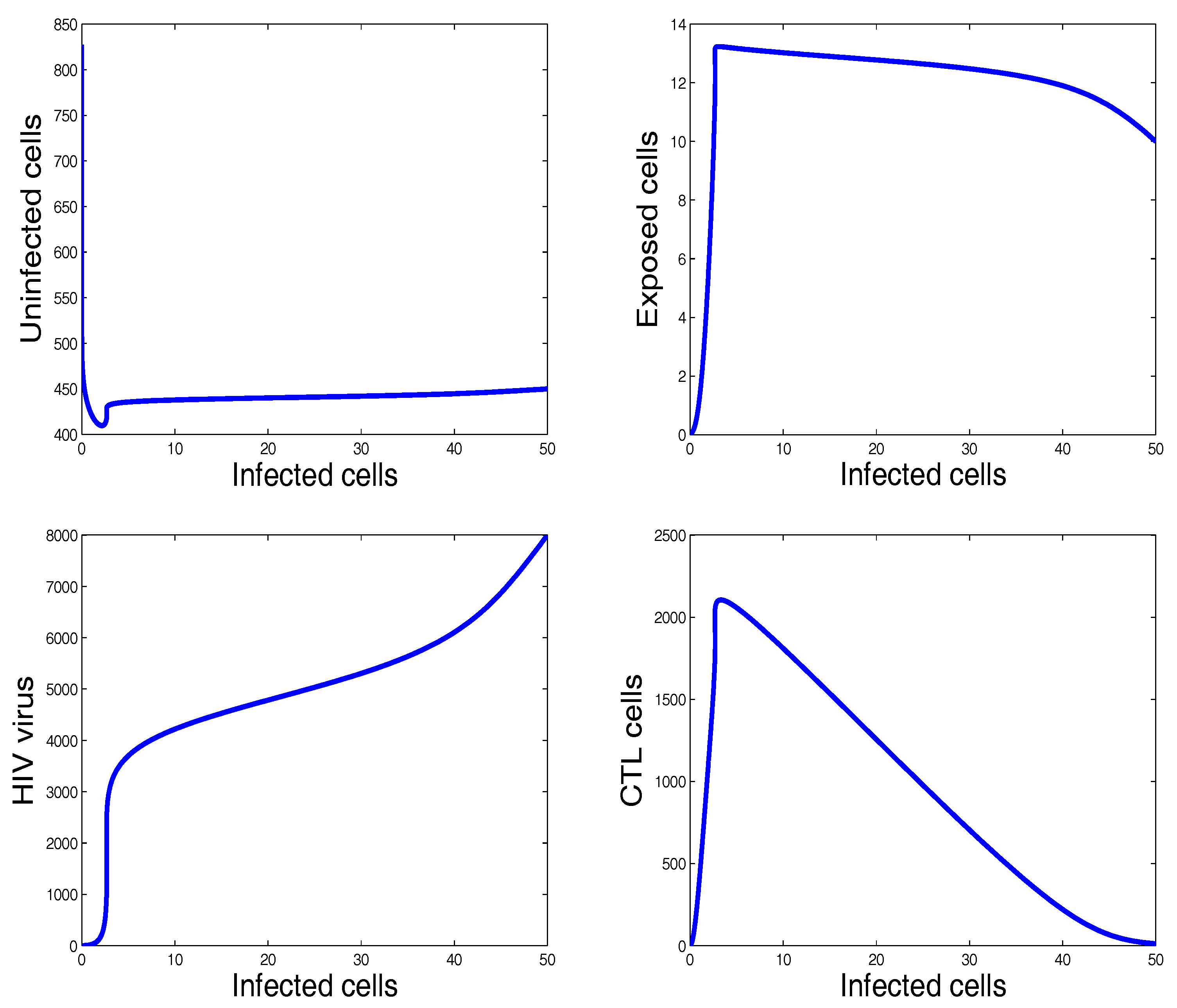
Figure 4 shows the behavior of the infection for the first sixty days. The chosen parameters in this figure ensure that the basic reproduction number is greater than unity () and the immune response reproduction number is less than unity (). It is clearly seen that, in this case, all the solutions converge towards the CTL-free endemic equilibrium that agrees with our theoretical finding concerning the stability of . Moreover, the plots showing the stability of this CTL-free endemic point in phase plane are given in Figure 5.
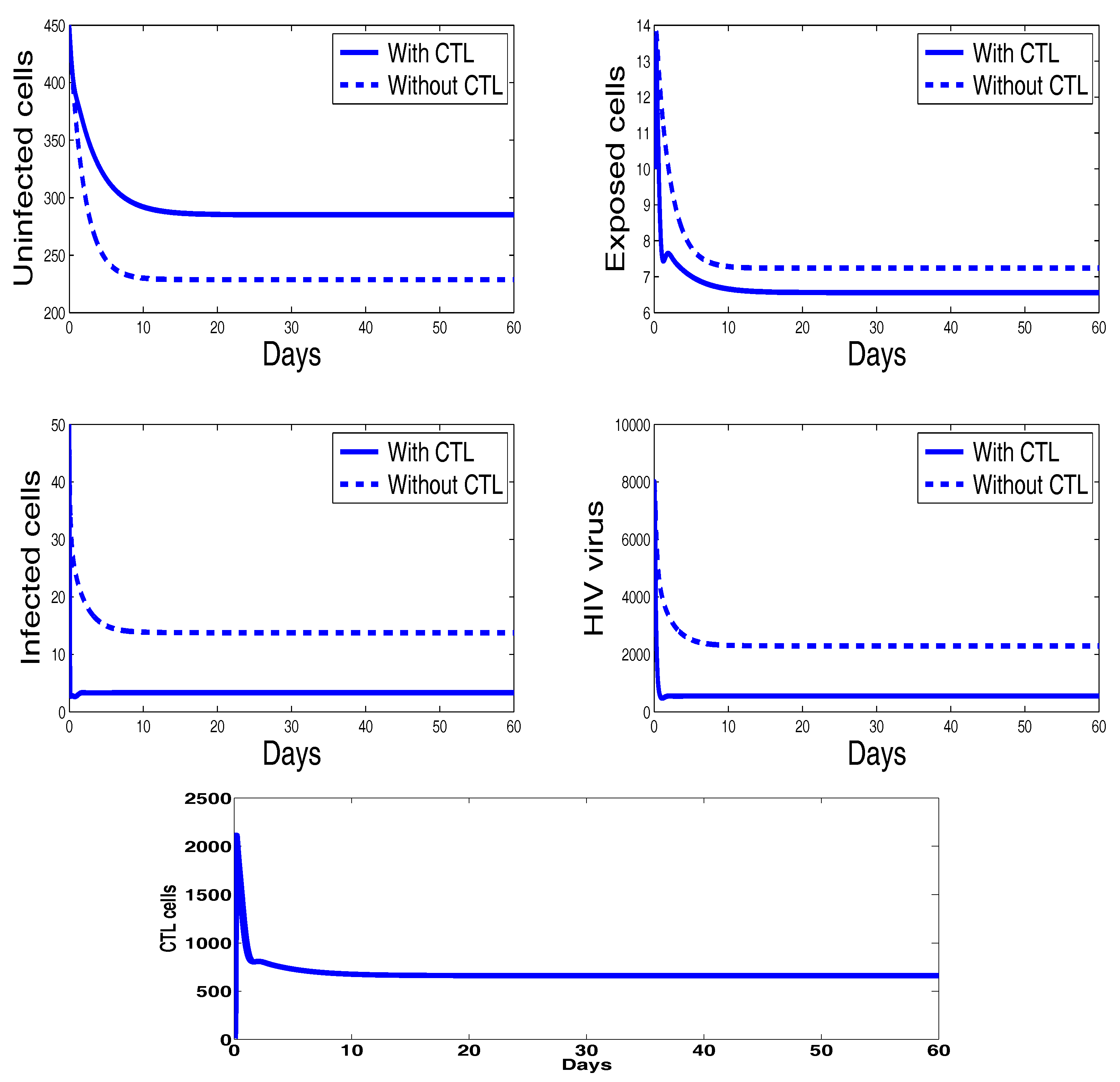
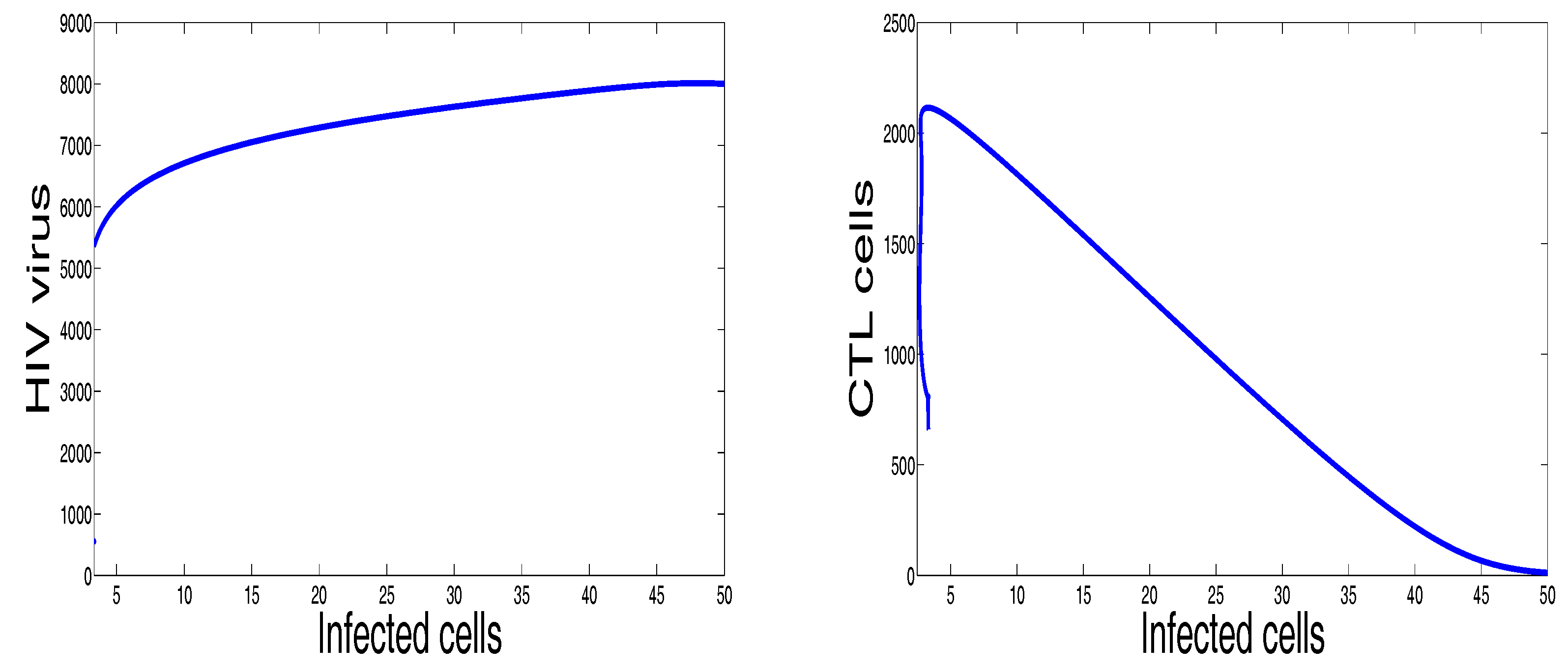
Finally, Figure 6 illustrates the disease dynamics when both the basic reproduction number and the immune response reproduction number are greater than unity. Indeed, for the chosen parameters in this figure, we have and . It can be seen that the infection persists and the convergence towards the infection steady state is observed. This numerical result is in good agreement with the theoretical result concerning the stability of the last endemic equilibrium. The plots showing the stability of this final endemic point in phase plane are given in Figure 7. In these two last figures, we clearly observe the importance of CTL immune response in maximizing the healthy cells and reducing the viral load. It is also noteworthy that the CTLs do not vanish in this last case, which means that CTL cells will be always present when the infection becomes chronic.
4. Discussion
The HIV dynamics involving the density uninfected cells, the density of the infected cells, the density of HIV virus and the amount of CTL cells have been widely studied by means of a different mathematical model starting from the work in 1996 by Nowak and Bangham [5] and two years later in 1998 by [18]. Later, many mathematical approaches were developed in order to better understand the complex dynamics of the fatal HIV disease.
Recently, in 2015, Conway and Perelson [19] studied the same issue by incorporating the treatment into the HIV model. Motivated by all those previous works treating the dynamics of HIV along with the CTL immune response, we have incorporated the CTL effect to a model suggested recently in 2015 by Sun et al. [14], in which the authors studied HIV dynamics by incorporating into the model the treatment and a more realistic incidence functional that describes the infection rate taking into account the crowd of the free viruses near the uninfected cells. In the latter work, the uninfected cells need time to become infected after HIV virus contact. Indeed, there exists an eclipse phase that is needed for the exposed CD4 T cells to become infected (see Figure 1). In this paper, we have taken into account this phase and we have added the CTL immune response to the model.
In this paper, we have established the well-posedness of the suggested model that ensures that all the solutions exist and are bounded. This agrees with the biological reality that the total cell amounts of these populations are bounded. Moreover, three steady states of the problem are found and their local and global stability results are determined depending on the basic reproduction number and the CTL immune response reproduction number .
We have also presented some numerical results that confirm our theoretical findings. In addition, several plots of the solutions in phase diagrams have been drawn in order to illustrate the stability of the three steady states.
The model dynamics indicate that the immune response represented by the cytotoxic T lymphocytes is efficient in controlling viral replication. Indeed, our numerical results show that, in the endemic case (see Figure 6), the CTL immune response plays an essential role in maximizing the effect of the uninfected CD4 T cells, minimizing the amount of the infected cells and reducing the HIV viral load.
5. Conclusions
In this paper, we have studied the model of the HIV dynamics in the presence of the immune response, which is represented by the cytotoxic T lymphocytes (CTL) cells. The model describes the interaction between the healthy cells, the infected cells in eclipse phase, the productively infected cells and the immune cells. The model includes also a saturated rates in order to better describe the viral infection. The positiveness and the boundedness of solutions are established. In addition, we have studied the stability of both disease-free equilibrium and endemic equilibria. The disease free steady state is locally and globally asymptotically stable when the basic reproduction number is less than unity (). The existence of two other infection steady states when is established. The global stability of these endemic steady states depends on the basic reproduction number and the CTL immune response reproduction number . Numerical simulations are performed in order to show the behavior of infection during the days of observation. The theoretical and the numerical results are in good agreement. In addition, our model based results suggest that the system immunity represented by CTL can control viral replication and reduce the infection under appropriate conditions.
Acknowledgments
The authors would like to thank the three reviewers for their many helpful suggestions. Karam Allali is grateful to the support from the Moroccan American Commission for Educational and Cultural Exchange through the Fulbright Program and the hospitality of the School of Mathematical and Statistical Sciences of Arizona State University. Yang Kuang is partially supported by US NSF grants DMS-1518529 and DMS-1615879.
Author Contributions
Karam Allali and Yang Kuang discussed the idea of the work during the visit of the first at the Arizona State University. Karam Allali, Jaouad Danane and Yang Kuang wrote the paper. Karam Allali and Jaouad Danane carried out the numerical simuations.
Conflicts of Interest
The authors declare no conflict of interest.
Appendix A. Existence and Local Stability Results Proof
The proof of the existence result (Proposition 1) is as follows. First, by the classical differential equations theory, we can confirm that system (1) has a unique local solution in .
First, the solution is strictly positive for all . Indeed, assume the contrary, and let be the first time such that and . From the first equation of system (1), we have , which presents a contradiction. Therefore, for all . We also have the following:
and
This shows that , , and for all . On the other hand, for the boundedness of the solutions, assume first that
then, we will have
where . Therefore,
By the same reasoning, concerning the fourth equation, we will have
For the last equation, we will have
from which, we will have
this proves that the solutions , , , and are bounded. Hence, every local solution can be prolonged up to any time , which means that the solution exists globally.
For the local stability result (Proposition 2), the proof is stated as follows.
At the disease-free equilibrium, , the Jacobian matrix is given as follows:
The characteristic polynomial of is
Therefore,
and the two obvious first eigenvalues of the matrix are and , which are non-positive. Denoting
it is easy to check that we have always , and . In addition, it is easy to see that when . From the Routh–Hurwitz criterion, it follows that is locally asymptotically stable.
Appendix B. Global Stability Result Proof
The global stability proof of the endemic point (Proposition 3) is given as follows. Consider the following Lyapunov function:
The time derivative is given by:
If , then . Moreover, when . The largest compact invariant is
according to LaSalle’s invariance principle, , the limit system of equations is
We define another Lyapunov function and for implicity, using the same notation,
Since , then
since the arithmetic mean is greater than or equal to the geometric mean, it follows that
therefore, and the equality holds if and , which completes the proof. ☐
The global stability proof of the endemic point (Proposition 4) is given as follows. We employ the following Lyapunov function:
We have
On the other hand, we have
Hence,
and
Since
we have
Therefore,
which implies that
since the arithmetic mean is greater than or equal to the geometric mean, it follows that
In addition, when , we will have , which means that , and the equality hods when , , and . By the LaSalle invariance principle, the endemic point is globally stable when . ☐
Finally, the global stability proof of the endemic point (Proposition 5) is given as follows. We employ the following Lyapunov function:
We have
Since,
we have
On the other hand, we have
and
All of these imply
Again, since the arithmetic mean is greater than or equal to the geometric mean, it follows that
which means that , and the equality hods when , , , and . By the LaSalle invariance principle, the endemic point is globally stable. ☐
References
- Blanttner, W.; Gallo, R.C.; Temin, H.M. HIV causes aids. Science 1988, 241, 515–516. [Google Scholar] [CrossRef]
- Weiss, R.A. How does HIV cause AIDS? Science 1993, 260, 1273–1279. [Google Scholar] [CrossRef] [PubMed]
- Saez-Cirion, A.; Lacabaratz, C.; Lambotte, O.; Versmisse, P.; Urrutia, A.; Boufassa, F.; Barre-Sinoussi, F.; Delfraissy, J.F.; Sinet, M.; Pancino, G.; et al. HIV controllers exhibit potent CD8 T cell capacity to suppress HIV infection ex vivo and peculiar cytotoxic T-lymphocyte activation phenotype. Proc. Natl. Acad. Sci. USA 2007, 104, 6776–6781. [Google Scholar] [CrossRef] [PubMed]
- Betts, M.R.; Nason, M.C.; West, S.M.; De Rosa, S.C.; Migueles, S.A.; Abraham, J.; Lederman, M.M.; Benito, J.M.; Goepfert, P.A.; Connors, M.; et al. HIV nonprogressors preferentially maintain highly functional HIV-specific CD8+ T-cells. Blood 2006, 107, 4781–4789. [Google Scholar] [CrossRef] [PubMed]
- Nowak, M.A.; Bangham, C.R.M. Population dynamics of immune responses to persistent viruses. Science 1996, 272, 74–79. [Google Scholar] [CrossRef] [PubMed]
- Smith, H.L.; De Leenheer, P. Virus dynamics: A global analysis. SIAM J. Appl. Math. 2003, 63, 1313–1327. [Google Scholar] [CrossRef]
- Korobeinikov, A. Global properties of basic virus dynamics models. Bull. Math. Biol. 2004, 66, 879–883. [Google Scholar] [CrossRef] [PubMed]
- Daar, E.S.; Moudgil, T.; Meyer, R.D.; Ho, D.D. Transient highlevels of viremia in patients with primary human immunodeficiency virus type 1 infection. N. Engl. J. Med. 1991, 324, 961–964. [Google Scholar] [CrossRef] [PubMed]
- Kahn, J.O.; Walker, B.D. Acute human immunodeficiency virus type 1 infection. N. Engl. J. Med. 1998, 339, 33–39. [Google Scholar] [CrossRef] [PubMed]
- Kaufmann, G.R.; Cunningham, P.; Kelleher, A.D.; Zauders, J.; Carr, A.; Vizzard, J.; Law, M.; Cooper, D.A. Patterns of viral dynamics during primary human immunodeficiency virus type 1 infection. J. Infect. Dis. 1998, 178, 1812–1815. [Google Scholar] [CrossRef] [PubMed]
- Schacker, T.; Collier, A.; Hughes, J.; Shea, T.; Corey, L. Clinical and epidemiologic features of primary HIV infection. Ann. Int. Med. 1996, 125, 257–264. [Google Scholar] [CrossRef] [PubMed]
- Wang, X.; Elaiw, A.; Song, X. Global properties of a delayed HIV infection model with CTL immune response. Appl. Math. Comput. 2012, 218, 9405–9414. [Google Scholar] [CrossRef]
- Wang, X.; Tao, Y.; Song, X. Global stability of a virus dynamics model with Beddington-DeAngelis incidence rate and CTL immune response. Nonlinear Dyn. 2011, 66, 825–830. [Google Scholar] [CrossRef]
- Sun, Q.; Min, L.; Kuang, Y. Global stability of infection-free state and endemic infection state of a modified human immunodeficiency virus infection model. IET Syst. Biol. 2015, 9, 95–103. [Google Scholar] [CrossRef] [PubMed]
- Sun, Q.; Min, L. Dynamics Analysis and Simulation of a Modified HIV Infection Model with a Saturated Infection Rate. Comput. Math. Methods Med. 2014, 2014, 145162. [Google Scholar] [CrossRef] [PubMed]
- Wang, Y.; Zhou, Y.; Wu, J.; Heffernan, J. Oscillatory viral dynamics in a delayed HIV pathogenesis model. Math. Biosci. 2009, 219, 104–112. [Google Scholar] [CrossRef] [PubMed]
- Zhu, H.; Luo, Y.; Chen, M. Stability and Hopf bifurcation of a HIV infection model with CTL-response delay. Comput. Math. Appl. 2011, 62, 3091–3102. [Google Scholar] [CrossRef]
- De Boer, R.J.; Perelson, A.S. Target cell limited and immune control models of HIV infection: A comparison. J. Theor. Biol. 1998, 190, 201–214. [Google Scholar] [CrossRef] [PubMed]
- Conway, J.M.; Perelson, A.S. Post-treatment control of HIV infection. Proc. Natl. Acad. Sci. USA 2015, 112, 5467–5472. [Google Scholar] [CrossRef] [PubMed]
Figure 1.
Schematic of the model under consideration.

Figure 2.
The behavior of the infection dynamics for , , , , , , , , , , . For the parameters used in this figure, the basic reproduction number is Solutions of the system converge to the disease-free equilibrium point .
Figure 2.
The behavior of the infection dynamics for , , , , , , , , , , . For the parameters used in this figure, the basic reproduction number is Solutions of the system converge to the disease-free equilibrium point .

Figure 3.
Selective phase portraits to illustrate the solution behavior of the infection dynamics when , , , , , , , , , , .
Figure 3.
Selective phase portraits to illustrate the solution behavior of the infection dynamics when , , , , , , , , , , .

Figure 4.
The behavior of the infection dynamics for , , , , , , , , , , . For the parameters used in this figure, the basic reproduction number is The immune response reproduction number In this case, all the solutions converge towards the endemic equilibrium
Figure 4.
The behavior of the infection dynamics for , , , , , , , , , , . For the parameters used in this figure, the basic reproduction number is The immune response reproduction number In this case, all the solutions converge towards the endemic equilibrium


Figure 5.
Selective phase portraits to illustrate the solution behavior of the infection dynamics when , , , , , , , , , , .
Figure 5.
Selective phase portraits to illustrate the solution behavior of the infection dynamics when , , , , , , , , , , .

Figure 6.
The behavior of the infection dynamics for , , , , , , , , , , . For the chosen parameters in this figure, we have and . Solutions tending to the infection steady state are observed.
Figure 6.
The behavior of the infection dynamics for , , , , , , , , , , . For the chosen parameters in this figure, we have and . Solutions tending to the infection steady state are observed.

Figure 7.
Selective phase portraits to illustrate the solution behavior of the infection dynamics when , , , , , , , , , , .
Figure 7.
Selective phase portraits to illustrate the solution behavior of the infection dynamics when , , , , , , , , , , .


Table 1.
Parameters, their symbols and default values used in the suggested HIV model.
| Parameters | Meaning | Value | References |
|---|---|---|---|
| Source rate of CD4 T cells | [16] | ||
| Average of infection | [14] | ||
| Decay rate of healthy cells | [14] | ||
| Death rate of exposed CD4 T cells | [14] | ||
| The rate that exposed become infected CD4 T cells | [14] | ||
| Death rate of infected CD4 T cells, not by CTL killing | [14] | ||
| a | The rate of production the virus by infected CD4 T cells | [14] | |
| Clearance rate of virus | [14] | ||
| p | Clearance rate of infection | [17] | |
| c | Activation rate CTL cells | [17] | |
| b | Death rate of CTL cells | [17] |
© 2017 by the authors. Licensee MDPI, Basel, Switzerland. This article is an open access article distributed under the terms and conditions of the Creative Commons Attribution (CC BY) license (http://creativecommons.org/licenses/by/4.0/).
Share and Cite
MDPI and ACS Style
Allali, K.; Danane, J.; Kuang, Y. Global Analysis for an HIV Infection Model with CTL Immune Response and Infected Cells in Eclipse Phase. Appl. Sci. 2017, 7, 861. https://doi.org/10.3390/app7080861
AMA Style
Allali K, Danane J, Kuang Y. Global Analysis for an HIV Infection Model with CTL Immune Response and Infected Cells in Eclipse Phase. Applied Sciences. 2017; 7(8):861. https://doi.org/10.3390/app7080861
Chicago/Turabian StyleAllali, Karam, Jaouad Danane, and Yang Kuang. 2017. "Global Analysis for an HIV Infection Model with CTL Immune Response and Infected Cells in Eclipse Phase" Applied Sciences 7, no. 8: 861. https://doi.org/10.3390/app7080861
Note that from the first issue of 2016, this journal uses article numbers instead of page numbers. See further details here.